Vehicle Ownership and Income Growth, Worldwide: 1960-2030

Joyce Dargay, Dermot Gately and Martin Sommer

July 2006

Abstract: The speed of vehicle ownership expansion in emerging market and developing countries has important implications for transport and environmental policies, as well as the global oil market. The literature remains divided on the issue of whether the vehicle ownership rates will ever catch up to the levels common in the advanced economies. This paper contributes to the debate by building a model that explicitly models the vehicle saturation level as a function of observable country characteristics: urbanization and population density. Our model is estimated on the basis of pooled time-series (1960-2002) and cross-section data for 45 countries that include 75 percent of the world’s population. We project that the total vehicle stock will increase from about 800 million in 2002 to over 2 billion units in 2030. By this time, 56% of the world’s vehicles will be owned by non-OECD countries, compared with 24% in 2002. In particular, China’s vehicle stock will increase nearly twenty-fold, to 390 million in 2030. This fast speed of vehicle ownership expansion implies rapid growth in oil demand. Keywords: vehicle ownership, transport modeling, oil market. JEL Classification: O12 - Microeconomic Analyses of Economic Development;

R41 - Transportation: Demand, Supply, and Congestion; Q41 – Energy Demand and Supply.

Joyce Dargay Institute for Transport Studies, University of Leeds Leeds LS2 9JT, England j.dargay@its.leeds.ac.uk Corresponding Author: Dermot Gately Dept. of Economics, New York University 269 Mercer St., New York, NY 10003 USA Dermot.Gately@NYU.eduTelephone: 212 998 8955 Fax: 212 995 3932 Martin Sommer International Monetary Fund 700 19th St. NW, Washington, DC 20431 USA MSommer@imf.org

1

1. INTRODUCTION Economic development has historically been strongly associated with an increase in the demand for transportation and particularly in the number of road vehicles. This relationship is also evident in the developing economies today. Surprisingly, very little research has been done on the determinants of vehicle ownership in developing countries. Typically, researchers make assumptions about vehicle saturation rates (IEA, 2005, or OPEC, 2004), which are very much lower than the vehicle ownership already experienced in the most of the wealthier countries. Because of this, their forecasts of future vehicle ownership in currently developing countries are much lower than would be expected by comparison with developed countries when these were at comparable income levels. This paper empirically estimates the saturation rate for different countries, by formalizing the idea that vehicle saturation levels may be different across countries. Given data availability, we limit ourselves to the influence of demographic factors, urban population and population density. A higher proportion of urban population and greater population density would encourage the availability and use of public transit, and could reduce the distances traveled by individuals and for goods transportation. Thus countries that are more urbanized and densely populated could have a lower need for vehicles. In this study we attempt to account for these demographic differences by specifying a country’s saturation level as a function its population density and proportion of the population living in urban areas. There are, of course, a number of other reasons why saturation may vary amongst countries. For example, the existence of reliable public transport alternatives and the use of rail for goods transport may reduce the saturation demand for road vehicles. Alternatively, investment in a comprehensive road network will most likely increase the saturation level. Such factors, however, are difficult to take into account, as they would require far more data than are available for all but a few countries. This paper examines the trends in the growth of the stock of road vehicles (at least 4 wheels) for a large sample of countries since 1960 and makes projections of its development through 2030. It employs an S-shaped function – the Gompertz function – to estimate the relationship between vehicle ownership and per-capita income, or GDP. Pooled time-series and cross-section data are employed to estimate empirically the responsiveness of vehicle ownership to income growth at different income levels. By employing a dynamic model specification, which takes into account lags in adjustment of the vehicle stock to income changes, the influence of income on the vehicle stock over time is examined. The estimates are used, in conjunction with forecasts of income and population growth, for projections of future growth in the vehicle stock. The study builds on the earlier work of Dargay and Gately (1999), who estimated vehicle demand in a sample of 26 countries - 20 OECD countries and 6 developing countries – for the period 1960 to 1992, and projected vehicle ownership rates until 2015. The current study extends that work in four ways. Firstly, we relax the 1999 paper’s assumption of a common saturation level for all countries. In our previous study, the

2

estimated saturation level was constrained to be the same for all countries (at about 850 vehicles per thousand people); differences in vehicle ownership between countries at the same income level were accounted for by allowing saturation to be reached at different income levels. Secondly, the data set is extended in time to 2002 and adds 19 countries (mostly non-OECD countries) to the original 26; these 45 countries comprise about three-fourths of world population. The inclusion of a large number of non-OECD countries – more than one-third of the countries, with three-fourths of the sample’s population – provides a high degree of variation in both income and vehicle ownership. This allows more precise estimates of the relationship between income and vehicle ownership at various stages of economic development. In addition, the model is used for countries not included in the econometric analysis to obtain projections for the “rest of the world”. The third extension we make to our earlier study concerns the assumption of symmetry in the response of vehicle ownership to rising and falling income. Given habit persistence, the longevity of the vehicle stock and expectations of rising income, one might expect that reductions in income would not lead to changes in vehicle ownership of the same magnitude as those resulting from increasing income. If this is the case, estimates based on symmetric models can be misleading if there is a significant proportion of observations where income declines. This is the case in the current study, particularly for developing countries. In most countries, real per capita income has fallen occasionally, and in Argentina and South Africa it has fallen over a number of years. In order to account for possible asymmetry, the demand function is specified so that the adjustment to falling income can be different from that to rising income. Specifically, the model permits the short-run response to be different for rising and falling income without changing the equilibrium relationship between the vehicle stock and income. The hypothesis of asymmetry is then tested statistically. Finally, the fourth extension is to use the projections of vehicle growth to investigate the implications for future transportation oil demand. This is based on a number of simplifying assumptions and comparisons are made with other projections. Section 2 summarizes the data used for the analysis, and explores the historical patterns of vehicle ownership and income growth. Section 3 presents the Gompertz model used in the econometric estimation, and the econometric results are described in Section 4. Section 5 summarizes the projections for vehicle ownership, based upon assumed growth rates of per-capita income in the various countries. Section 6 presents the implications for the growth of highway fuel demand. Section 7 presents conclusions.

3

2. HISTORICAL PATTERNS IN THE GROWTH OF VEHICLE OWNERSHIP

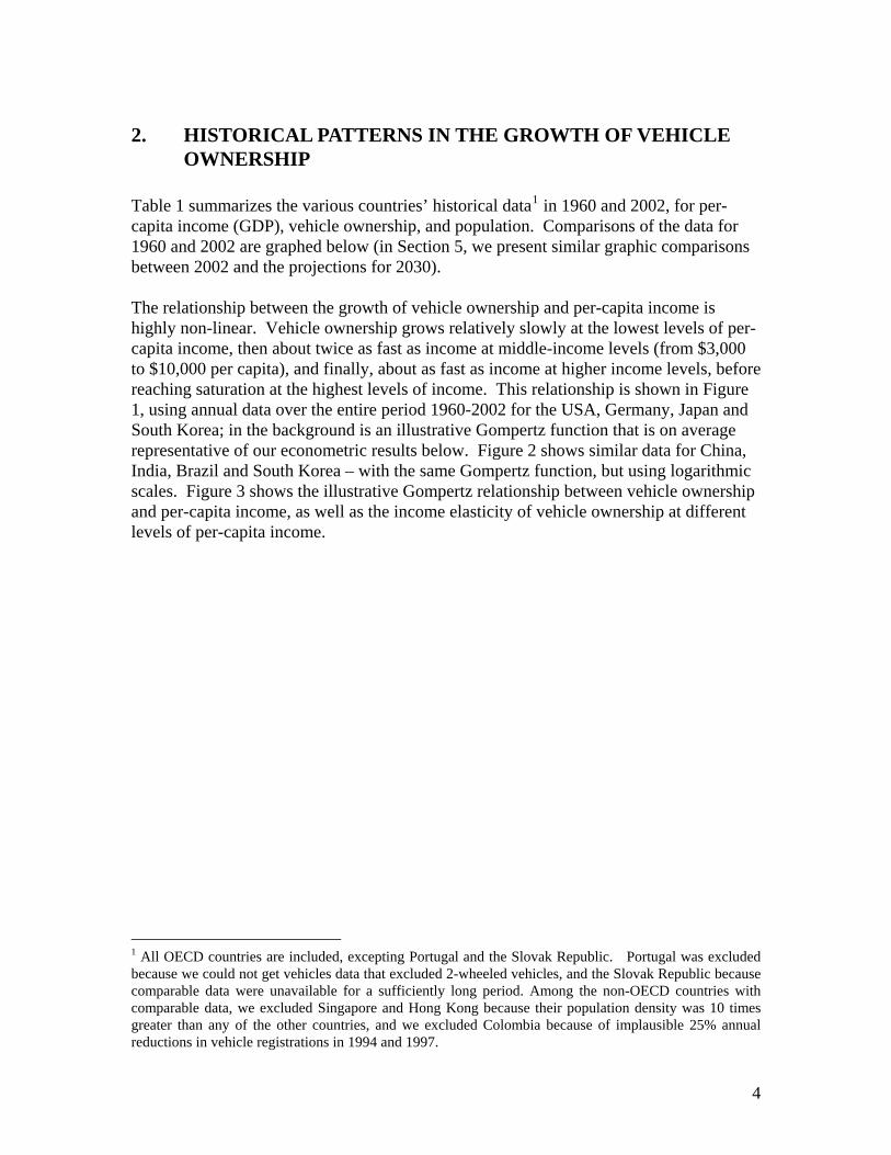
Table 1 summarizes the various countries’ historical data1 in 1960 and 2002, for per-capita income (GDP), vehicle ownership, and population. Comparisons of the data for 1960 and 2002 are graphed below (in Section 5, we present similar graphic comparisons between 2002 and the projections for 2030). The relationship between the growth of vehicle ownership and per-capita income is highly non-linear. Vehicle ownership grows relatively slowly at the lowest levels of per-capita income, then about twice as fast as income at middle-income levels (from $3,000 to $10,000 per capita), and finally, about as fast as income at higher income levels, before reaching saturation at the highest levels of income. This relationship is shown in Figure 1, using annual data over the entire period 1960-2002 for the USA, Germany, Japan and South Korea; in the background is an illustrative Gompertz function that is on average representative of our econometric results below. Figure 2 shows similar data for China, India, Brazil and South Korea – with the same Gompertz function, but using logarithmic scales. Figure 3 shows the illustrative Gompertz relationship between vehicle ownership and per-capita income, as well as the income elasticity of vehicle ownership at different levels of per-capita income.

1 All OECD countries are included, excepting Portugal and the Slovak Republic. Portugal was excluded because we could not get vehicles data that excluded 2-wheeled vehicles, and the Slovak Republic because comparable data were unavailable for a sufficiently long period. Among the non-OECD countries with comparable data, we excluded Singapore and Hong Kong because their population density was 10 times greater than any of the other countries, and we excluded Colombia because of implausible 25% annual reductions in vehicle registrations in 1994 and 1997.

4

Country Codefirst data year (if

not 1960)

1960 or

first year

2002Average annual

growth rate

1960 or

first year

2002Average annual

growth rate

1960 or first year

2002Average annual

growth ratemillions

density per

sq.KM

% urbanized

OECD, North AmericaCanada Can 10.4 26.9 2.3% 292 581 1.6% 5.2 18.2 3.0% 0.72 31 3 79United States USA 13.1 31.9 2.1% 411 812 1.6% 74.4 233.9 2.8% 0.76 288 31 78Mexico Mex 3.7 8.1 1.9% 22 165 4.9% 0.8 16.7 7.5% 2.58 101 53 75

OECD, EuropeAustria Aut 8.1 26.3 2.8% 69 629 5.4% 0.5 5.1 5.8% 1.91 8 97 68Belgium Bel 8.2 24.7 2.7% 102 520 4.0% 0.9 5.3 4.3% 1.48 10 315 97Switzerland Che 15.4 27.7 1.4% 106 559 4.0% 0.6 4.0 4.8% 2.89 7 184 67Czech Republic Cze 1970 8.9 13.6 1.3% 82 390 5.0% 0.8 4.0 5.1% 3.79 10 133 75Germany Deu 9.0 23.5 2.3% 73 586 5.1% 5.1 48.3 5.5% 2.20 83 236 88Denmark Dnk 10.6 25.9 2.1% 126 430 3.0% 0.6 2.3 3.4% 1.38 5 127 85Spain Esp 4.8 19.3 3.3% 14 564 9.2% 0.4 22.9 9.9% 2.74 41 82 78Finland Fin 7.4 24.3 2.9% 58 488 5.2% 0.3 2.5 5.6% 1.82 5 17 59France Fra 8.5 23.7 2.5% 158 576 3.1% 7.2 35.3 3.9% 1.26 61 108 76Great Britain GBr 9.7 23.6 2.1% 137 515 3.2% 7.2 30.6 3.5% 1.50 59 246 90Greece Grc 4.5 16.1 3.1% 10 422 9.4% 0.1 4.6 10.1% 3.03 11 82 61Hungary Hun 1963 4.2 12.3 2.8% 15 306 8.1% 0.1 3.0 8.1% 2.87 10 110 65Ireland Ire 5.3 29.8 4.2% 78 472 4.4% 0.2 1.9 5.2% 1.05 4 57 60Iceland Isl 8.3 26.7 2.8% 118 672 4.2% 0.0 0.2 5.4% 1.50 0.3 3 93Italy Ita 7.2 23.3 2.8% 49 656 6.4% 2.5 37.7 6.7% 2.25 57 196 67Luxembourg Lux 10.9 42.6 3.3% 135 716 4.0% 0.05 0.3 4.7% 1.23 0.4 173 92Netherlands Nld 9.6 25.3 2.3% 59 477 5.1% 0.7 7.7 5.9% 2.19 16 477 90Norway Nor 7.7 28.1 3.1% 95 521 4.1% 0.3 2.4 4.7% 1.33 5 15 75Poland Pol 4.0 9.6 2.1% 8 370 9.5% 0.2 14.4 10.3% 4.51 39 127 63Sweden Swe 10.2 25.4 2.2% 175 500 2.5% 1.3 4.5 3.0% 1.15 9 22 83Turkey Tur 2.5 6.1 2.1% 4 96 7.7% 0.1 6.4 10.0% 3.62 67 90 67

OECD, PacificAustralia Aus 10.4 25.0 2.1% 266 632 2.1% 2.7 12.5 3.7% 0.99 20 3 91Japan Jpn 4.5 23.9 4.1% 19 599 8.6% 1.8 76.3 9.4% 2.12 127 349 79Korea Kor 1.4 15.1 5.8% 1.2 293 13.9% 0.03 13.9 15.7% 2.40 48 483 83New Zealand NZL 11.1 19.6 1.4% 271 612 2.0% 0.6 2.4 3.2% 1.45 4 15 86

Non-OECD, South AmericaArgentina Arg 1962 9.7 9.6 -0.05% 55 186 3.1% 0.9 7.1 5.4% -67.8 38 13 88Brazil Bra 1962 2.7 7.1 2.5% 20 121 4.6% 1.0 20.8 7.8% 1.87 171 21 82Chile Chl 1962 1.8 9.2 4.2% 17 144 5.4% 0.1 2.2 7.5% 1.29 16 21 86Dominican Rep. Dom 1962 2.3 6.0 2.4% 7 118 7.3% 0.02 1.0 10.7% 3.04 9 178 67Ecuador Ecu 1969 1.7 2.9 1.6% 9 50 5.2% 0.03 0.7 10.1% 3.16 13 46 64

Non-OECD, Africa and Middle EastEgypt Egy 1963 1.2 3.5 2.8% 4 38 6.0% 0.1 2.5 8.4% 2.16 68 67 43Israel Isr 1961 3.3 17.9 4.2% 25 303 6.2% 0.1 1.9 9.3% 1.49 6 318 92Morocco Mar 1962 2.1 3.6 1.3% 17 59 3.2% 0.2 1.8 6.0% 2.44 30 66 57Syria Syr 1.2 3.1 2.4% 6 35 4.1% 0.03 0.6 7.5% 1.71 17 92 52South Africa Zaf 1962 6.7 8.8 0.7% 66 152 2.1% 1.1 6.9 4.7% 3.17 45 37 58

Non-OECD, AsiaChina Chn 1962 0.3 4.3 6.5% 0.38 16 9.8% 0.2 20.5 12.0% 1.51 1285 137 38Chinese Taipei Twn 1974 3.8 18.5 5.0% 14 260 9.5% 0.2 5.9 12.4% 1.89 23 701 81Indonesia Idn 0.7 2.9 3.3% 2.1 29 6.4% 0.2 6.2 8.6% 1.93 216 117 43India Ind 0.9 2.3 2.3% 1.0 17 6.8% 0.4 17.4 9.1% 2.92 1051 353 28Malaysia Mys 1967 2.2 8.1 3.8% 25 240 6.7% 0.2 5.9 9.6% 1.77 25 74 59Pakistan Pak 0.9 1.8 1.8% 1.7 12 4.7% 0.1 1.7 7.4% 2.57 145 188 34Thailand Tha 1.0 6.2 4.4% 4 127 8.7% 0.1 8.1 11.0% 1.98 64 121 20

Sample (45 countries) 3.4 8.6 2.3% 53 166 2.8% 118 728 4.4% 1.21 4346 68 48Other Countries 2.2 3.1 0.8% 5 45 5.2% 4 83 7.4% 6.73 1891 28 45

OECD Total 8.1 22.12 2.4% 150 550 3.1% 115 617 4.1% 1.30 1127 34 78Non-OECD Total 1.4 3.6 2.3% 4 39 5.6% 9 195 7.5% 2.39 5110 53 41

Total World 3.1 7.0 2.0% 41 130 2.8% 122 812 4.6% 1.41 6237 48 47

Population, 2002per-capita GDP (thousands, real, PPP)

Vehicles per 1000 population ratio of

growth rates:

Veh.Own. to per-cap.

GDP

Total Vehicles (millions)

Table 1. Historical Data on Income, Vehicle Ownership and Population, 1960-2002

5

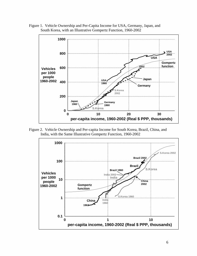
Figure 1. Vehicle Ownership and Per-Capita Income for USA, Germany, Japan, and South Korea, with an Illustrative Gompertz Function, 1960-2002

0 10 20 30per-capita income, 1960-2002 (Real $ PPP, thousands)

0

200

400

600

800

1000

Vehiclesper 1000people

1960-2002

USA

Japan

S.Korea

GermanyS.Korea2002

2002

USA2002

USA1960

Germany1960

Japan1960

Gompertzfunction

Figure 2. Vehicle Ownership and Per-capita Income for South Korea, Brazil, China, and

India, with the Same Illustrative Gompertz Function, 1960-2002

0 1 10per-capita income, 1960-2002 (Real $ PPP, thousands)

0.1

1

10

100

1000

Vehiclesper 1000people

1960-2002

India

China

S.KoreaBrazil

Brazil 2002

China2002

1962

S.Korea 1960India1960

S.Korea 2002

Brazil 1960

India 2002

Gompertzfunction

6

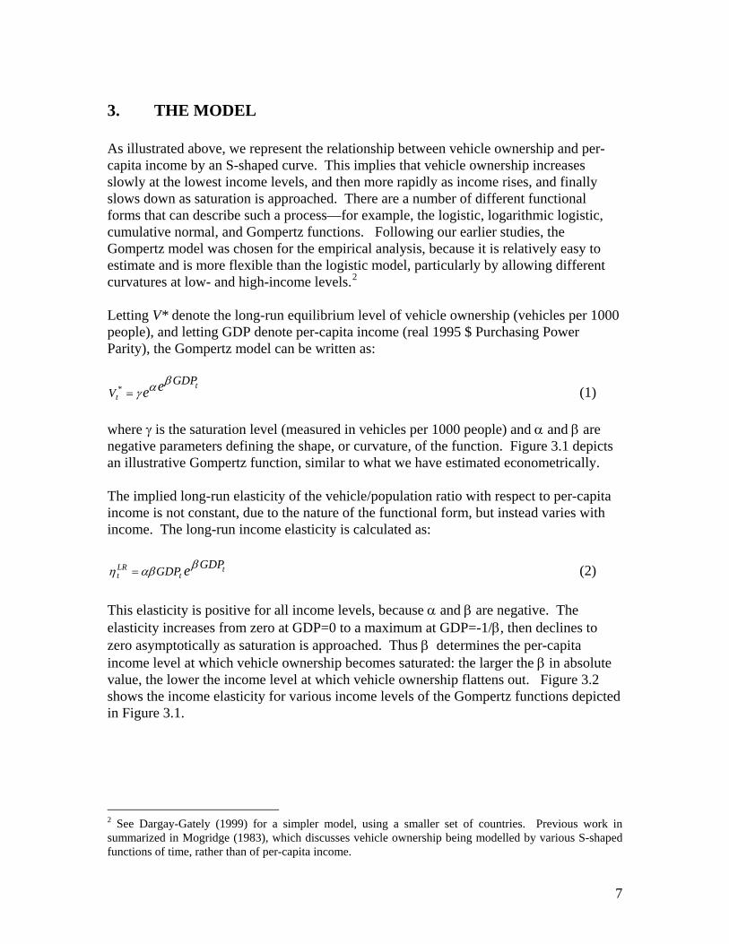
3. THE MODEL As illustrated above, we represent the relationship between vehicle ownership and per-capita income by an S-shaped curve. This implies that vehicle ownership increases slowly at the lowest income levels, and then more rapidly as income rises, and finally slows down as saturation is approached. There are a number of different functional forms that can describe such a process—for example, the logistic, logarithmic logistic, cumulative normal, and Gompertz functions. Following our earlier studies, the Gompertz model was chosen for the empirical analysis, because it is relatively easy to estimate and is more flexible than the logistic model, particularly by allowing different curvatures at low- and high-income levels.2 Letting V* denote the long-run equilibrium level of vehicle ownership (vehicles per 1000 people), and letting GDP denote per-capita income (real 1995 $ Purchasing Power Parity), the Gompertz model can be written as:

t

t

GDPV ee

βαγ=* (1) where γ is the saturation level (measured in vehicles per 1000 people) and α and β are negative parameters defining the shape, or curvature, of the function. Figure 3.1 depicts an illustrative Gompertz function, similar to what we have estimated econometrically. The implied long-run elasticity of the vehicle/population ratio with respect to per-capita income is not constant, due to the nature of the functional form, but instead varies with income. The long-run income elasticity is calculated as:

tt

LRt

GDPGDP eβαβη = (2) This elasticity is positive for all income levels, because α and β are negative. The elasticity increases from zero at GDP=0 to a maximum at GDP=-1/β, then declines to zero asymptotically as saturation is approached. Thus β determines the per-capita income level at which vehicle ownership becomes saturated: the larger the β in absolute value, the lower the income level at which vehicle ownership flattens out. Figure 3.2 shows the income elasticity for various income levels of the Gompertz functions depicted in Figure 3.1.

2 See Dargay-Gately (1999) for a simpler model, using a smaller set of countries. Previous work in summarized in Mogridge (1983), which discusses vehicle ownership being modelled by various S-shaped functions of time, rather than of per-capita income.

7

Fig. 3.1 Illustrative Gompertz function

0 10 20 30 40 50

per-capita income (thousands)

0

100

200

300

400

500

600

700

800

900

1000

vehicleownership:

vehiclesper 1000people

Fig. 3.2 Implied Income Elasticity

0 10 20 30 40 50

per-capita income (thousands)

0

1

2

3

incomeelasticity

ofvehicle

ownership

We assume that the Gompertz function (1) describes the long-run relationship between vehicle ownership and per-capita income. In order to account for lags in the adjustment of vehicle ownership to per-capita income, a simple partial adjustment mechanism is postulated:

(3) )( 1

*1 −− −+= tttt VVVV θ

where V is actual vehicle ownership and θ is the speed of adjustment (0 < θ <1). Such lags reflect the slow adjustment of vehicle ownership to increased income: the necessary build-up of savings to afford ownership; the gradual changes in housing patterns and land use that are associated with increased ownership; and the slow demographic changes as young adults learn to drive, replacing their elders who have never driven. Substituting equation (1) into equation (3), we have the equation:

1)1( −−+= tt

t VGDP

V ee θβ

θγ α (4) In Dargay and Gately (1999), we had assumed that only the coefficients βi were country-specific, while all the other parameters of the Gompertz function were the same for all countries: the saturation level γ, the speed of adjustment θ, and the coefficient α. Thus, differences between countries were reflected in the curvature parameters βi , which determined the income level for each country at which the common level of saturation is reached. In this paper we relax this restriction of a common saturation level. Instead, we assume that the maximum saturation level will be that estimated for the USA, denoted

MAXγ . Other countries that are more urbanized and more densely populated than the

8

USA will have lower saturation levels. The saturation level for country i at time t is specified as:3

otherwiseUUifUUU

andotherwise

DDifDDD

whereUD

tUSAittUSAitit

tUSAittUSAitit

ititMAXit

0

0

,,

,,

=

>−=

=

>−=

++= ϕλγγ

(5)

where λ and ϕ are negative.

Figure 4. Countries’ Population Density and Urbanization, 2002

Figure 4 plots the 2002 data on population density and urbanization. The most urbanized and densely populated countries are in Western Europe and East Asia: Netherlands, Belgium, Germany, Great Britain, Japan and South Korea. Some countries are highly urbanized but not densely populated, such as Australia and Canada. Others are densely populated but not highly urbanized, such as China, India, Pakistan, Thailand, and Indonesia.

0 20 40 60 80 100

% Urbanized, 2002

1

10

100

1000

PopulationDensity

2002(per sq. KM,log scale)

Chn

Ind

USA

Idn

Bra

Pak

Jpn

Mex

Deu

EgyTur

Tha Fra

GBrIta

Kor

Zaf

Esp

Pol

Arg

Can

MarMys

Twn

Aus

Syr

Nld

Chl

Ecu

Grc

Bel

CzeHun

Swe

Dom

Aut

Che

Isr

Dnk

Fin Nor NZL

Ire

Lux

Isl

The dynamic specification in equations (3) and (4) assumes that the response to a fall in income is equal but opposite the response to an equivalent rise in income. As mentioned earlier, there is a good deal of evidence that this may not be the case, and that assuming symmetry may lead to biased estimates of income elasticities. Since many of the countries in the sample have experienced negative as well as positive per-capita income growth over the period (especially Argentina and South Africa), it is important that we take such asymmetry into consideration.4 To do so, the adjustment coefficient relating to periods of falling income, θF , is allowed to be different from that to rising income, θR. This is done by creating two dummy variables defined as:

3 Population density and urbanization are normalised by taking the deviations from their means over all countries and years in the data sample. Since population density and urbanization vary over time, so too does the saturation level. 4 This issue had been addressed previously in Dargay (2001).

9

otherwiseandGDP GDP ifFotherwiseandGDP GDP ifR

ititit

ititit

001001

1

1

=<−==>−=

−

− (6)

and replacing θ in (4) with:

itFitR FR θθθ += (7) This specification does not change the equilibrium relationship between the vehicle stock and income given in equation (1), nor the long-run income elasticities. Only the rate of adjustment to equilibrium is different for rising and falling income, so that the short-run elasticities and the time required for adjustment will be different. Since it is likely that vehicle ownership does not decline as quickly when income falls as it increases when income rises, we would expect θR > θF . The hypothesis of asymmetry can be tested statistically from the estimates of θR and θF. If they are not statistically different from each other, symmetry cannot be rejected and the model reverts to the traditional, symmetric case. Substituting (5) and (7) into (4), the model to be estimated econometrically from the pooled data sample becomes:

itititFitR

iti

itFitRititMAXit VFRGDPeeFRUDV εθθ

βαθθϕλγ +−−++++= −1)1())(( (8) where the subscript i represents country i and εit is random error term. The adjustment parameters, θR and θF , and the parameters α, γ , ϕ and λ are constrained to be the same for all countries, while βi is allowed to be country-specific, as is each country’s saturation level from equation (5). The long-run income elasticities for each country are calculated as

itiiti

LRti

GDPeGDP ββαη = (9) which are the same as in the symmetric model (2). The short-run income elasticities are also determined by the adjustment parameter, θ, and are

itiiti

SRit

GDPeGDP ββαθη = . (10) where θ = θR for income increases and θ = θF for income decreases. The rationale for pooling time-series data across countries is the following. Although it is possible, in theory, to estimate a separate vehicle ownership function for each country, the short time periods and relatively small range of income levels that are available for each country make such an approach untenable. Reliable estimation of the saturation level requires observations on vehicle ownership which are nearing saturation.

10

Analogously, estimation of the parameter α, which determines the value of the Gompertz function at the lowest income levels, necessitates observations for low income and ownership levels. Thus it would not be sensible to estimate the saturation level for low-income countries separately, because vehicle ownership in these countries is far from saturation. Similarly, one could not estimate the lower end of the curve, i.e. the parameter α, on the basis of data only for high-income countries with high vehicle-ownership, unless historic data were available for many years in the past. For these reasons, we use a pooled time-series cross-section approach, with all countries being modeled simultaneously. We had considered utilizing additional explanatory variables in the model, such as the cost of vehicle ownership, or the price of gasoline.5 However, the unavailability of data for a sufficient number of countries and periods prevented such an attempt.

5 Storchmann (2005) uses fuel price, the fixed cost of vehicle ownership, and income distribution – but not per-capita income – to explain vehicle ownership across countries. His data set includes more countries (90) but only a short time series, 1990-1997.

11

4. MODEL ESTIMATION The model described in equation (8) was estimated for the cross-section time-series data for the 45 countries. The period of estimation is generally from 1960 to 2002, but is shorter for some countries due to early data being unavailable (see Table 1). In all, we have 1838 observations. In order to allow larger countries to have more influence on the estimated coefficients, the observations were weighted with population. As mentioned above, the maximum saturation level, MAXγ , the speed-of-adjustment coefficients, θR and θF, and the lower-curvature parameter α were constrained to be the same for all countries. The upper-curvature parameters βi were estimated separately for each country. The model was estimated using iterative least squares. The resulting estimates are shown in Table 2. A total of 51 parameters are estimated, including 45 country-specific βi. All the estimated coefficients are of the expected signs: θR , θF , and MAXγ are positive and α, λ, ϕ and βi are negative. All coefficients are statistically significant, except for the βi coefficients for Luxembourg, Iceland, Ecuador, and Syria. From the Adjusted R2, we see the model explains the data very well; however, this is to be expected in a model containing a lagged dependent variable. The estimated adjustment parameter is larger for rising income than for falling income, 0.095 versus 0.084. Testing the equality θR = θF yields an F-statistic of 4.76 (with probability value=0.03) so that symmetry is rejected. This implies that the vehicle stock responds less quickly when income falls than when income rises. With increasing income, 9.5% of the complete adjustment occurs in one year, but when income falls only 8.4% of the long-term adjustment occurs in one year. Thus a fall in per-capita income reduces vehicle ownership about 11% less in the short run (1-year) than an equivalent rise in income increases vehicle ownership. The long-run elasticity is the same for both income increases and decreases.

12

Table 2. Estimated Coefficients of Equation (8) coef. P-value

Speed of adjustment θincome increases 0.095 0.0000income decreases 0.084 0.0000

max. saturation level γ max 852 0.0000population density λ -0.000388 0.0000urbanization φ -0.007765 0.0001alpha α -5.897 0.0000

Country Code beta coef. P-valuevehicle

ownership saturation

per-capita GDP (in thousands) at which vehicle ownership =

200

OECD, North AmericaCanada Can -0.15 0.00 845 9.4United States USA -0.20 0.00 852 7.0Mexico Mex -0.17 0.00 840 7.9

OECD, EuropeAustria Aut -0.15 0.00 831 9.4Belgium Bel -0.20 0.00 647 8.1Switzerland Che -0.11 0.00 803 13.3Czech Republic Cze -0.17 0.00 819 8.3Germany Deu -0.18 0.00 728 8.5Denmark Dnk -0.12 0.00 782 12.0Spain Esp -0.17 0.00 835 8.1Finland Fin -0.13 0.00 852 10.6France Fra -0.15 0.00 823 9.4Great Britain GBr -0.17 0.00 707 8.9Greece Grc -0.15 0.00 836 9.4Hungary Hun -0.17 0.00 831 8.1Ireland Ire -0.15 0.01 841 9.4Iceland Isl -0.17 0.87 779 8.3Italy Ita -0.18 0.00 800 8.1Luxembourg Lux -0.16 0.78 706 9.6Netherlands Nld -0.16 0.00 613 10.1Norway Nor -0.13 0.00 852 10.6Poland Pol -0.23 0.00 821 6.2Sweden Swe -0.13 0.00 825 10.6Turkey Tur -0.18 0.00 820 7.7

OECD, PacificAustralia Aus -0.19 0.00 785 7.7Japan Jpn -0.18 0.00 732 8.3Korea Kor -0.20 0.00 646 8.1New Zealand NZL -0.19 0.01 812 7.3

Non-OECD, South AmericaArgentina Arg -0.13 0.00 800 10.6Brazil Bra -0.17 0.00 831 8.5Chile Chl -0.17 0.00 810 8.3Dominican Rep. Dom -0.24 0.02 777 6.2Ecuador Ecu -0.25 0.13 845 5.6

Non-OECD, Africa and Middle EastEgypt Egy -0.22 0.00 824 6.3Israel Isr -0.13 0.00 630 12.6Morocco Mar -0.25 0.00 830 5.6Syria Syr -0.22 0.22 807 6.5South Africa Zaf -0.14 0.00 852 10.1

Non-OECD, AsiaChina Chn -0.14 0.00 807 10.1Chinese Taipei Twn -0.16 0.00 508 11.7Indonesia Idn -0.23 0.00 808 6.3India Ind -0.24 0.00 683 6.5Malaysia Mys -0.23 0.00 827 6.0Pakistan Pak -0.21 0.01 725 7.3Thailand Tha -0.22 0.00 812 6.3

Adjusted R-squared 0.999821Sum of Squared Residuals 0.038947

13

The estimated maximum saturation level is 852 vehicles per 1000 people – for the USA and for those countries which are less urbanized and less densely populated: Finland, Norway, and South Africa. The coefficients for population density and urbanization are both negative and statistically significant, indicating that the saturation level declines with increasing population density and with increasing urbanization. The lowest saturation levels among the large countries are for Netherlands, Belgium, Germany, Great Britain, Japan, South Korea and India. Figure 5 plots each country’s estimated saturation level and the income level at which it would reach vehicle ownership of 200 vehicles per 1000 people. The latter measures reflects the country’s curvature parameter βi. Some countries would reach vehicle ownership of 200 quickly, at relatively low income levels (USA, India, Indonesia, Malaysia), while others would reach it more slowly, at much higher income levels (China, Netherlands, Denmark, Israel, Switzerland). Fig. 5 Countries’ Estimated Vehicle Ownership Saturation Levels and Income Levels at which Vehicle Ownership = 200.

ArgAus

Aut

Bel

BraCan

CheChl ChnCze

Deu

DnkDom

EcuEgy Esp

Fin

Fra

GBr

GrcHunIdn

Ind

Ire

Isl

Isr

Ita

Jpn

Kor

Lux

Mar MexMys

Nld

Nor

NZL

Pak

Pol SweSyrTha Tur

Twn

USA Zaf

0 2 4 6 8 10 12 14

per-capita GDP at which vehicle ownership = 200 in long run

400

500

600

700

800

900

vehicleownershipsaturation

level

The value of α determines the maximum income elasticity of vehicle ownership rates6, which in this case is estimated to be 2.1. The value of βi determines the income level where the common maximum elasticity is reached: the smaller the βi in absolute value, the greater the per-capita income at which the maximum income elasticity occurs – for the different countries respectively, at income levels between $4,000 and $9,600. The vehicle ownership level at which the maximum income elasticity occurs is about 90 vehicles per 1000 people. The values of α and βi also determine the income level at which vehicle saturation is reached. The estimates imply that 99% of saturation is

6 The maximum elasticity is derived by setting the derivative of the long-run elasticity with respect to GDP equal to zero, solving for the value of GDP where the elasticity is a maximum and replacing this value of GDP (=-1/β) in the original elasticity formula. This gives a maximum elasticity of -αe-1 = -0.367α.

14

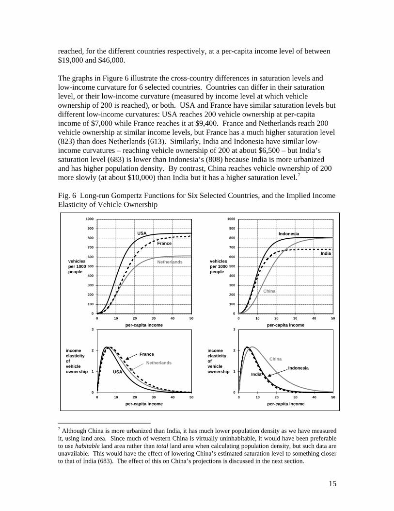
reached, for the different countries respectively, at a per-capita income level of between $19,000 and $46,000. The graphs in Figure 6 illustrate the cross-country differences in saturation levels and low-income curvature for 6 selected countries. Countries can differ in their saturation level, or their low-income curvature (measured by income level at which vehicle ownership of 200 is reached), or both. USA and France have similar saturation levels but different low-income curvatures: USA reaches 200 vehicle ownership at per-capita income of $7,000 while France reaches it at $9,400. France and Netherlands reach 200 vehicle ownership at similar income levels, but France has a much higher saturation level (823) than does Netherlands (613). Similarly, India and Indonesia have similar low-income curvatures – reaching vehicle ownership of 200 at about $6,500 – but India’s saturation level (683) is lower than Indonesia’s (808) because India is more urbanized and has higher population density. By contrast, China reaches vehicle ownership of 200 more slowly (at about $10,000) than India but it has a higher saturation level.7 Fig. 6 Long-run Gompertz Functions for Six Selected Countries, and the Implied Income Elasticity of Vehicle Ownership

0 10 20 30 40 50

per-capita income

0

100

200

300

400

500

600

700

800

900

1000

vehiclesper 1000people

USA

France

Netherlands

0 10 20 30 40 50

per-capita income

0

100

200

300

400

500

600

700

800

900

1000

vehiclesper 1000people

Indonesia

India

China

0 10 20 30 40 50

per-capita income

0

1

2

3

incomeelasticityofvehicleownership

0 10 20 30 40 50

per-capita income

0

1

2

3

incomeelasticityofvehicleownershipUSA

France

NetherlandsIndonesia

India

China

7 Although China is more urbanized than India, it has much lower population density as we have measured it, using land area. Since much of western China is virtually uninhabitable, it would have been preferable to use habitable land area rather than total land area when calculating population density, but such data are unavailable. This would have the effect of lowering China’s estimated saturation level to something closer to that of India (683). The effect of this on China’s projections is discussed in the next section.

15

5. PROJECTIONS OF VEHICLE OWNERSHIP TO 2030

On the basis of assumptions concerning future trends in income, population and urbanization, the model projects vehicle ownership for each country.8 These are shown in Table 3 and graphed in figures that follow. Within the OECD countries, projected growth in vehicle ownership is relatively slow, about 0.6% annually, because many of these countries are approaching saturation. The only exceptions to slowly growing vehicle ownership in the OECD are Mexico and Turkey, whose vehicle ownership will grow faster than income. However, due to population growth, the annual growth rate for total OECD vehicles is somewhat higher, at 1.4%. For the USA, we project only a slight increase in vehicle ownership (from 812 to 849 per 1000 people) but a large absolute increase in the total vehicle stock of 80 million, due to population growth of nearly 1% annually. This 80 million increase for the USA is larger than the projected 2030 total of vehicles in any European country, and is almost as large as the total number of vehicles in Japan. For the non-OECD countries9, we project much faster rates of growth: vehicle ownership growth of about 3.5% annually, and total vehicles growth of 6.5% annually – four times the rate for the OECD. The most rapid growth is in the non-OECD economies with high rates of income growth, and per-capita income levels ($3,000 to $10,000) at which the income elasticity of vehicle ownership is the highest. China has by far the highest growth rate of vehicle ownership, 10.6% annually, followed by India (7%) and Indonesia (6.5%). By 2030, China will have 269 vehicles per 1000 people – comparable to vehicle ownership levels of Japan and Western Europe in the early 1970’s – and it will have more vehicles than any other country: 24% more vehicles than the USA. China’s vehicle ownership is projected to grow rapidly for two reasons: (1) its projected high growth rate for per-capita income during 2002-2030, 4.8% (which is actually much slower than its recent rapid growth), and (2) vehicle ownership is growing 2.2 times as fast as per-capita income, as it passes through the middle level of per-capita income ($3,000 to $10,000) with the highest income-elasticity of vehicle ownership. Similarly for India and

8 Population density is assumed to grow at the same rate as population. Projections for urbanization are obtained by estimating a model relating urbanization to per-capita income and lagged urbanization for all countries over the sample period and creating forecasts on the basis of this model and the projected per-capita income values. The model used and the estimates obtained are available upon request. 9 For the “Other” (non-sample) countries in the rest of the world, we projected vehicle ownership from our estimated Gompertz function’s parameters, adapted to this “Other” group’s characteristics. In 2002 this group had per-capita income of about $3000 and owned 44 vehicles per 1000 people. We estimated the group’s βi coefficient by regressing the sample countries’ βi values against the levels of per-capita income at which the respective countries had 44 vehicles per 1000 people; this produced a value of βi=-0.21 for “Other” countries. Using the sample countries’ median saturation value (812), we assumed 2.5% annual per-capita income growth for “Other” countries, and projected their vehicle ownership to 2030.

16

Indonesia, whose per-capita income is not projected to grow as fast as China’s, but whose vehicle ownership is projected to grow nearly twice as fast as per-capita income. The faster growth of total vehicles in the non-OECD countries will more than double their share of world vehicles – from 24% in 2002 to 56% by 2030. Non-OECD countries will acquire over three-fourths of these additional vehicles – nearly 30% will be from China alone. By 2030, there will be 2.08 billion vehicles on the planet, compared with 812 million in 2002; this total is 2.5 times greater than in 2002. The historical results shown in the left graphs of Figure 7 indicate quite rapid growth in vehicle ownership within the OECD, and in many non-OECD countries as well, over the period 1970-2002, when their vehicle ownership doubles or triples. In many countries, vehicle ownership frequently grew twice as fast as per-capita income, and in a few countries more than twice as fast. Such large income-elasticities for vehicle ownership (two or higher) are consistent with the non-linear Gompertz function we have estimated, for countries whose per-capita income is increasing through the middle-income range of $3,000 to $10,000. The projected results, in the right graphs of Figure 7, show that most OECD countries’ vehicle ownership growth will decelerate in the future, growing at a rate lower than per-capita income. However, the non-OECD countries whose per-capita income is increasing through the middle-income range will experience growth in vehicle ownership that is at least as rapid as their growth in per-capita income. In some of the largest countries, vehicle ownership will grow twice as rapidly as per-capita income – in China, India, Indonesia, and Egypt. Figure 8 compares these historical and projected ratios of vehicle ownership growth to per-capita income growth. Figure 9 summarizes the historical and projected changes in total vehicles.

17

Table 3. Projections of Income and Vehicle Ownership, 2002-2030

Country Code 2002 2030Average annual

growth rate2002 2030

Average annual

growth rate2002 2030

Average annual

growth rate2002 2030

Average annual

growth rate

OECD, North AmericaCanada Can 26.9 46.2 2.0% 581 812 1.2% 18.2 30.0 1.8% 0.62 31 37 0.6%United States USA 31.9 56.6 2.1% 812 849 0.2% 234 314 1.1% 0.08 288 370 0.9%Mexico Mex 8.1 19.3 3.1% 165 491 4.0% 16.7 65.5 5.0% 1.26 101 134 1.0%

OECD, EuropeAustria Aut 26.3 49.8 2.3% 629 803 0.9% 5.1 6.4 0.8% 0.38 8 8 -0.1%Belgium Bel 24.7 45.3 2.2% 520 636 0.7% 5.3 6.7 0.8% 0.33 10 11 0.1%Switzerland Che 27.7 54.3 2.4% 559 741 1.0% 4.0 4.9 0.7% 0.41 7 7 -0.3%Czech Republic Cze 13.6 40.2 4.0% 390 740 2.3% 4.0 7.1 2.1% 0.59 10 10 -0.2%Germany Deu 23.5 38.1 1.7% 586 705 0.7% 48.3 57.5 0.6% 0.38 83 82 0.0%Denmark Dnk 25.9 46.7 2.1% 430 715 1.8% 2.3 3.9 1.9% 0.86 5 5 0.1%Spain Esp 19.3 39.0 2.5% 564 795 1.2% 22.9 31.7 1.2% 0.48 41 40 -0.1%Finland Fin 24.3 46.1 2.3% 488 791 1.7% 2.5 4.2 1.8% 0.75 5 5 0.0%France Fra 23.7 41.2 2.0% 576 779 1.1% 35.3 50.3 1.3% 0.54 61 65 0.2%Great Britain GBr 23.6 43.1 2.2% 515 685 1.0% 30.6 44.0 1.3% 0.47 59 64 0.3%Greece Grc 16.1 33.0 2.6% 422 725 2.0% 4.6 7.7 1.8% 0.75 11 11 -0.1%Hungary Hun 12.3 40.0 4.3% 306 745 3.2% 3.0 6.4 2.7% 0.75 10 9 -0.5%Ireland Ire 29.8 54.0 2.1% 472 812 2.0% 1.9 3.9 2.7% 0.91 4 5 0.7%Iceland Isl 26.7 49.5 2.2% 672 768 0.5% 0.2 0.3 1.0% 0.21 0 0 0.5%Italy Ita 23.3 44.5 2.3% 656 781 0.6% 37.7 40.2 0.2% 0.27 57 52 -0.4%Luxembourg Lux 42.6 63.8 1.4% 716 706 -0.1% 0.3 0.4 1.1% -0.04 0 1 1.1%Netherlands Nld 25.3 42.3 1.8% 477 593 0.8% 7.7 10.2 1.0% 0.42 16 17 0.2%Norway Nor 28.1 47.5 1.9% 521 805 1.6% 2.4 4.0 1.9% 0.83 5 5 0.3%Poland Pol 9.6 30.7 4.2% 370 746 2.5% 14.4 27.4 2.3% 0.60 39 37 -0.2%Sweden Swe 25.4 48.1 2.3% 500 777 1.6% 4.5 7.0 1.6% 0.69 9 9 0.0%Turkey Tur 6.1 14.1 3.0% 96 377 5.0% 6.4 34.7 6.2% 1.67 67 92 1.2%

OECD, PacificAustralia Aus 25.0 47.6 2.3% 632 772 0.7% 12.5 18.4 1.4% 0.31 20 24 0.7%Japan Jpn 23.9 42.1 2.0% 599 716 0.6% 76.3 86.6 0.5% 0.31 127 121 -0.2%Korea Kor 15.1 39.0 3.5% 293 609 2.6% 13.9 30.5 2.8% 0.77 48 50 0.2%New Zealand NZL 19.6 39.1 2.5% 612 786 0.9% 2.4 3.5 1.3% 0.36 4 4 0.4%

Non-OECD, South AmericaArgentina Arg 9.6 25.5 3.6% 186 489 3.5% 7.1 23.8 4.4% 1.0 38 49 0.9%Brazil Bra 7.1 15.9 2.9% 121 377 4.1% 20.8 83.7 5.1% 1.43 171 222 0.9%Chile Chl 9.2 23.7 3.4% 144 574 5.1% 2.2 11.7 6.1% 1.47 16 20 0.9%Dominican Rep. Dom 6.0 13.6 3.0% 118 448 4.9% 1.0 5.1 5.9% 1.65 9 11 1.0%Ecuador Ecu 2.9 7.0 3.1% 50 182 4.7% 0.7 3.2 5.6% 1.50 13 17 0.9%

Non-OECD, Africa and Middle EastEgypt Egy 3.5 6.6 2.3% 38 142 4.9% 2.5 15.5 6.7% 2.09 68 109 1.7%Israel Isr 17.9 25.9 1.3% 303 454 1.5% 1.9 4.1 2.7% 1.10 6 9 1.3%Morocco Mar 3.6 7.5 2.7% 59 228 4.9% 1.8 9.7 6.3% 1.83 30 43 1.3%Syria Syr 3.1 4.9 1.6% 35 80 3.0% 0.6 2.3 4.9% 1.89 17 29 1.8%South Africa Zaf 8.8 18.6 2.7% 152 395 3.5% 6.9 16.7 3.2% 1.27 45 42 -0.3%

Non-OECD, AsiaChina Chn 4.3 16.0 4.8% 16 269 10.6% 20.5 390 11.1% 2.20 1285 1451 0.4%Chinese Taipei Twn 18.5 46.2 3.3% 260 477 2.2% 5.9 13.6 3.1% 0.66 23 29 0.8%Indonesia Idn 2.9 7.3 3.4% 29 166 6.5% 6.2 46.1 7.4% 1.89 216 278 0.9%India Ind 2.3 6.2 3.5% 17 110 7.0% 17.4 156 8.1% 1.98 1051 1417 1.1%Malaysia Mys 8.1 19.8 3.2% 240 677 3.8% 5.9 23.8 5.1% 1.16 25 35 1.3%Pakistan Pak 1.8 3.4 2.2% 12 29 3.2% 1.7 7.8 5.6% 1.48 145 272 2.3%Thailand Tha 6.2 18.3 3.9% 127 592 5.7% 8.1 44.6 6.3% 1.43 64 75 0.6%

Sample (45 countries) 8.6 18.3 1.8% 166 316 1.5% 728 1765 3.2% 0.85 4346 5379 0.8%Other Countries 3.0 6.0 1.7% 44 112 2.2% 83 315 4.9% 1.34 1891 2820 1.4%

OECD Total 22.3 41.6 1.5% 548 713 0.6% 617 908 1.4% 0.42 1127 1272 0.4%Non-OECD Total 3.6 9.1 2.2% 38 169 3.6% 195 1172 6.6% 1.61 5110 6927 1.1%

Population (millions)per-capita GDP (thousands, real, PPP)

Vehicles per 1000 population

Total Vehicles (millions)

ratio of growth rates:

Veh.Own. to per-cap.

GDP

Total World 7.0 14.1 1.7% 130 254 1.6% 812 2080 3.4% 0.94 6237 8199 1.0%

18

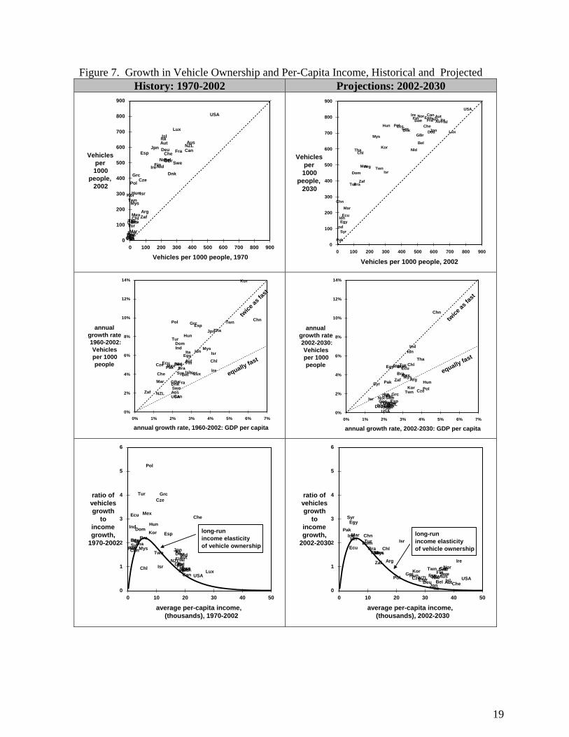
Figure 7. Growth in Vehicle Ownership and Per-Capita Income, Historical and Projected History: 1970-2002 Projections: 2002-2030

0 100 200 300 400 500 600 700 800 900

Vehicles per 1000 people, 1970

0

100

200

300

400

500

600

700

800

900

Vehiclesper1000

people,2002

ChnInd

USA

Idn

Bra

Pak

Jpn

Mex

Deu

Egy

TurTha

Fra

GBr

Ita

Kor

Zaf

Esp

Pol

Arg

Can

Mar

MysTwn

Aus

Syr

Nld

Chl

Ecu

Grc

Bel

Cze

Hun

Swe

Dom

Aut

Che

Isr

Dnk

FinNor

NZL

Ire

LuxIsl

800

700

600

500

400

300

200

100

0

900

Vehiclesper1000

people,2030

Chn

Ind

USA

Idn

Bra

Pak

Jpn

Mex

Deu

Egy

Tur

Tha

Fra

GBr

Ita

Kor

Zaf

Esp

Pol

Arg

Can

Mar

Mys

Twn

Aus

Syr

NldChl

Ecu

Grc

Bel

CzeHunSwe

Dom

Aut

Che

Isr

Dnk

FinNorNZL

Ire

Lux

Isl

0 100 200 300 400 500 600 700 800 900

Vehicles per 1000 people, 2002

0% 1% 2% 3% 4% 5% 6% 7%

annual growth rate, 1960-2002: GDP per capita

0%

2%

4%

6%

8%

10%

12%

14%

annualgrowth rate1960-2002:Vehiclesper 1000people

Chn

Ind

USA

Idn

BraPak

Jpn

MexDeu

Egy

Tur

Tha

FraGBr

Ita

Kor

Zaf

EspPol

Can

Mar

Mys

Twn

Aus

Syr

Nld ChlEcu

Grc

Bel

Cze

Hun

Swe

Dom

Aut

Che

Isr

Dnk

Fin

Nor

NZL

IreLuxIsl equally fast

twice

as fa

st

0% 1% 2% 3% 4% 5% 6% 7%

annual growth rate, 2002-2030: GDP per capita

0%

2%

4%

6%

8%

10%

12%

14%

annualgrowth rate2002-2030:Vehiclesper 1000people

Chn

Ind

USA

Idn

Bra

Pak

Jpn

Mex

Deu

Egy TurTha

FraGBrIta

Kor

Zaf

Esp

Pol

Arg

Can

Mar

Mys

Twn

Aus

Syr

Nld

ChlEcu

Grc

Bel

Cze

Hun

Swe

Dom

AutCheIsr

DnkFinNorNZL

Ire

Isl

equally fast

twice

as fa

st

0 10 20 30 40 50

average per-capita income,(thousands), 1970-2002

0

1

2

3

4

5

6

ratio ofvehiclesgrowth

toincomegrowth,

1970-2002Chn

Ind

USA

Idn

Bra

Pak Jpn

Mex

Deu

Egy

Tur

Tha

FraGBr

Ita

Kor Esp

Pol

Can

MarMys

Twn

Aus

Syr

Nld

Chl

Ecu

Grc

Bel

Cze

Hun

Swe

Dom

Aut

Che

Isr Dnk

Fin

Nor

NZL

Ire Lux

Isl

long-run income elasticityof vehicle ownership

0 10 20 30 40 50

average per-capita income,(thousands), 2002-2030

0

1

2

3

4

5

6

ratio ofvehiclesgrowth

toincomegrowth,

2002-2030ChnInd

USA

Idn

Bra

Pak

Jpn

Mex

Deu

Egy

Tur

Tha

FraGBr

Ita

Kor

Zaf

EspPol

ArgCan

Mar

Mys

TwnAus

Syr

Nld

ChlEcu

GrcBel

CzeHun Swe

Dom

AutChe

Isr

DnkFinNor

NZL

Ire

Isl

long-run income elasticityof vehicle ownership

19

Figure 8. Ratio of Growth Rate of Vehicle Ownership to Growth Rate of Per-Capita Income, Historical and Projected

0 1 2 3 4 5

ratio of growth rates: vehicle ownership to per-capita income, 1970-2002

0

1

2

3

4

5

ratio ofgrowthrates:

vehicleownership

toper-capita

income2002-2030

ChnInd

USA

Idn

Bra Pak

Jpn

Mex

Deu

Egy

TurTha

FraGBrIta

Kor

Zaf

EspPolCan

Mar

Mys

Twn

Aus

Syr

Nld

Chl Ecu

Grc

BelCze

HunSwe

Dom

Aut Che

IsrDnk FinNor

NZL

Ire

Isl

About half the countries experienced historical growth rates of vehicle ownership that are at least twice as high as the growth of per-capita income, and almost every country has had its vehicle ownership growing faster than per-capita income since 1970. However, for almost all countries the projected ratio of vehicle ownership growth to per-capita income growth will be lower than the historical ratio (below the diagonal in Figure 8). Yet there are important differences between OECD and non-OECD countries. For every OECD country except Mexico and Turkey, the projected ratio will be lower than 1. But for almost every non-OECD country, the projected ratio will be

higher than 1; and this ratio will be as high as 2 for China, India, Indonesia, Egypt, Syria, and Morocco – countries whose per-capita income will be passing through the middle-income range of $3,000 to $10,000, within which vehicle ownership grows twice as fast as per-capita income. Only when per-capita income levels rise above $15,000 can we expect vehicle ownership to grow no faster than per-capita income. Figure 9. Total Vehicles, Historical and Projected

History: 1970-2002 Projections: 2002-2030 400

1 2 3 4 5 6 7 8 910 20 30 40 50 60 708090100

200

300

400

# Vehicles (millions), 1970

1

2

3

45678910

20

30

405060708090100

200

300

# Vehicles(millions)

2002Ind

USA

Bra

Jpn

Mex

DeuFra

GBrIta

Zaf

Esp

Arg

Can

Aus

Nld

BelSweAut

Che

DnkNZL

400

1 2 3 4 5 6 7 8 910 20 30 40 50 60 708090100

200

300

400

300

200

# Vehicles (millions), 2002

1

2

3

45678910

20

30

405060708090100

# Vehicles(millions)

2030

Chn

Ind

USA

Idn

Bra

Pak

JpnMex Deu

Egy

TurTha FraGBrIta

Kor

Zaf

EspPol

ArgCan

Mar

Mys

TwnAus

NldChl

GrcBelCzeHunSwe

DomAut

CheIsrDnkFinNorNZLIre

By 2030, the six countries with the largest number of vehicles will be China, USA, India, Japan, Brazil, and Mexico. China is projected to have nearly 20 times as many vehicles in 2030 as it had in 2002. This growth is due both to its high rate of income growth and the fact that its per-capita income during this period is associated with vehicle ownership growing more than twice as fast as income.

20

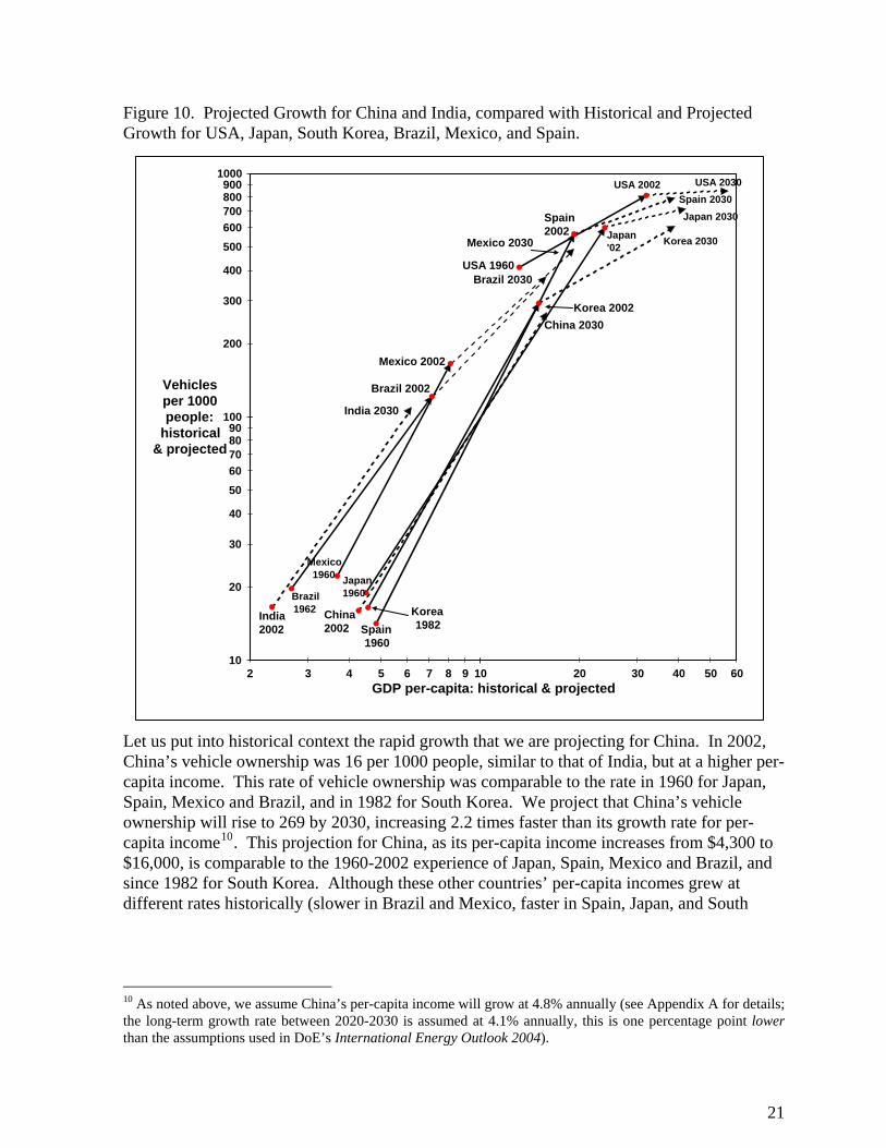
Figure 10. Projected Growth for China and India, compared with Historical and Projected Growth for USA, Japan, South Korea, Brazil, Mexico, and Spain.

2 3 4 5 6 7 8 9 10 20 30 40 50 60GDP per-capita: historical & projected

10

20

30

40

5060708090

100

200

300

400

500600700800900

1000

Vehiclesper 1000people:

historical& projected

USA 2030

India 2030

Korea1982

China2002

China 2030

Brazil1962

Mexico1960 Japan

1960

Brazil 2002

Mexico 2002

USA 1960

USA 2002

Korea 2030

Japan 2030

Japan'02

India2002

Brazil 2030

Spain1960

Spain2002

Spain 2030

Korea 2002

Mexico 2030

Let us put into historical context the rapid growth that we are projecting for China. In 2002, China’s vehicle ownership was 16 per 1000 people, similar to that of India, but at a higher per-capita income. This rate of vehicle ownership was comparable to the rate in 1960 for Japan, Spain, Mexico and Brazil, and in 1982 for South Korea. We project that China’s vehicle ownership will rise to 269 by 2030, increasing 2.2 times faster than its growth rate for per-capita income10. This projection for China, as its per-capita income increases from $4,300 to $16,000, is comparable to the 1960-2002 experience of Japan, Spain, Mexico and Brazil, and since 1982 for South Korea. Although these other countries’ per-capita incomes grew at different rates historically (slower in Brazil and Mexico, faster in Spain, Japan, and South

10 As noted above, we assume China’s per-capita income will grow at 4.8% annually (see Appendix A for details; the long-term growth rate between 2020-2030 is assumed at 4.1% annually, this is one percentage point lower than the assumptions used in DoE’s International Energy Outlook 2004).

21

Korea), their ratios of growth in vehicle ownership to per-capita income growth over the 1960-2002 period were at least as high as the 2.2 that we project for China.11

Figure 11. Total Vehicles, 1960-2030

1960 1970 1980 1990 2000 2010 2020 20300

200

400

600

800

1000

1200

1400

1600

1800

2000

2200

TotalVehicles(millions)

USA

Restof

OECD

China

History ProjectionsIndiaBrazil

Rest of Sample

Rest of World

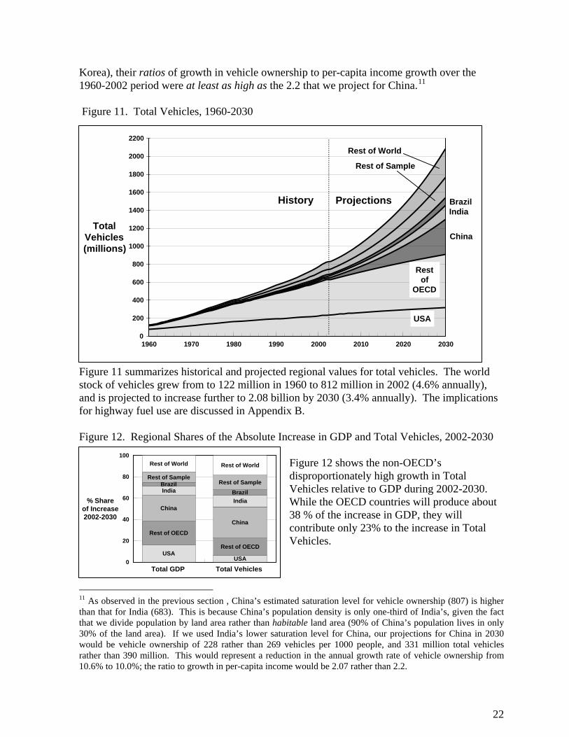
Figure 11 summarizes historical and projected regional values for total vehicles. The world stock of vehicles grew from to 122 million in 1960 to 812 million in 2002 (4.6% annually), and is projected to increase further to 2.08 billion by 2030 (3.4% annually). The implications for highway fuel use are discussed in Appendix B. Figure 12. Regional Shares of the Absolute Increase in GDP and Total Vehicles, 2002-2030

Total GDP Total Vehicles0

20

40

60

80

100

% Shareof Increase2002-2030

USAUSA

Rest of OECD

Rest of OECD

China

China

India

India

BrazilBrazil

Rest of SampleRest of Sample

Rest of World Rest of World Figure 12 shows the non-OECD’s disproportionately high growth in Total Vehicles relative to GDP during 2002-2030. While the OECD countries will produce about 38 % of the increase in GDP, they will contribute only 23% to the increase in Total Vehicles.

11 As observed in the previous section , China’s estimated saturation level for vehicle ownership (807) is higher than that for India (683). This is because China’s population density is only one-third of India’s, given the fact that we divide population by land area rather than habitable land area (90% of China’s population lives in only 30% of the land area). If we used India’s lower saturation level for China, our projections for China in 2030 would be vehicle ownership of 228 rather than 269 vehicles per 1000 people, and 331 million total vehicles rather than 390 million. This would represent a reduction in the annual growth rate of vehicle ownership from 10.6% to 10.0%; the ratio to growth in per-capita income would be 2.07 rather than 2.2.

22

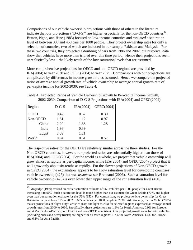
Comparisons of our vehicle ownership projections with those of others in the literature indicate that our projections (“D-G-S”) are higher, especially for the non-OECD countries12. Button, Ngoe, and Hine (1983) focused on low-income countries and assumed a saturation level of between 300 and 450 cars per 1000 people. They project ownership rates for only a selection of countries, two of which are included in our sample: Pakistan and Malaysia. For these two countries, they projected a doubling of cars from 1986 and 2002, but historical data show that vehicles have more than tripled over this time period. Hence their projections seem unrealistically low – the likely result of the low saturation levels that are assumed. More comprehensive projections for OECD and non-OECD regions are provided by IEA(2004) to year 2030 and OPEC(2004) to year 2025. Comparisons with our projections are complicated by differences in income growth rates assumed. Hence we compare the projected ratios of average annual growth rate of vehicle ownership to average annual growth rate of per-capita income for 2002-2030; see Table 4. Table 4. Projected Ratios of Vehicle Ownership Growth to Per-capita Income Growth,

2002-2030: Comparison of D-G-S Projections with IEA(2004) and OPEC(2004)

Region D-G-S IEA(2004) OPEC(2004)

OECD 0.42 0.57 0.39Non-OECD 1.61 1.12 0.97

China 2.20 1.38 1.28India 1.98 0.39

Egypt 2.09 1.21World 0.94 0.61 0.57

The respective ratios for the OECD are relatively similar across the three studies. For the Non-OECD countries, however, our projected ratios are substantially higher than those of IEA(2004) and OPEC(2004). For the world as a whole, we project that vehicle ownership will grow almost as rapidly as per-capita income, while IEA(2004) and OPEC(2004) project that it will grow only about six-tenths as rapidly. For the slower projections of Non-OECD growth in OPEC(2004), the explanation appears to be a low saturation level for developing countries’ vehicle ownership (425) that was assumed: see Brennand (2006). Such a saturation level for vehicle ownership (425) is even lower than upper range of the car saturation level (450) 12 Mogridge (1989) revised an earlier saturation estimate of 660 vehicles per 1000 people for Great Britain, increasing it to 900. Such a saturation level is much higher than our estimate for Great Britain (707), and higher even than our saturation estimate for the USA (852). For comparison, we project vehicle ownership for Great Britain to increase from 515 in 2002 to 685 vehicles per 1000 people in 2030. Additionally, Exxon Mobil (2005) makes projections of “light duty” vehicles (cars and light trucks) for selected regions expressed as average annual growth rates from 2000 to 2030. Specifically, these projections are 1.2% for North America, 0.9% for Europe, and 4.7% for Asia-Pacific (both OECD and non-OECD countries). Our projected growth rates for total vehicles (including buses and heavy trucks) are higher for all three regions: 1.7% for North America, 1.6% for Europe, and 6.1% for Asia Pacific.

23

assumed by Button et al (1983). As for the projections of IEA(2004), details of the underlying model are not provided. To sum up these comparisons, the considerably lower projections of non-OECD vehicle ownership in Button et al (1983) and in OPEC (2004) are due to the assumption of significantly lower saturation levels for those regions. This assumption leaves unexplained why developing countries – once they had achieved incomes similar to many OECD countries – would not have comparable levels of vehicle ownership. On what other goods would consumers in developing countries be spending their incomes instead?

24

1 10 100 1000

Vehicles per 1000 people, 1971-2002

0

1

2

3

4

5

Gasolineper

Vehicle1971-2002(gallonsper day)

China

Germany

Japan

USAS.Korea

India

Brazil

Mexico

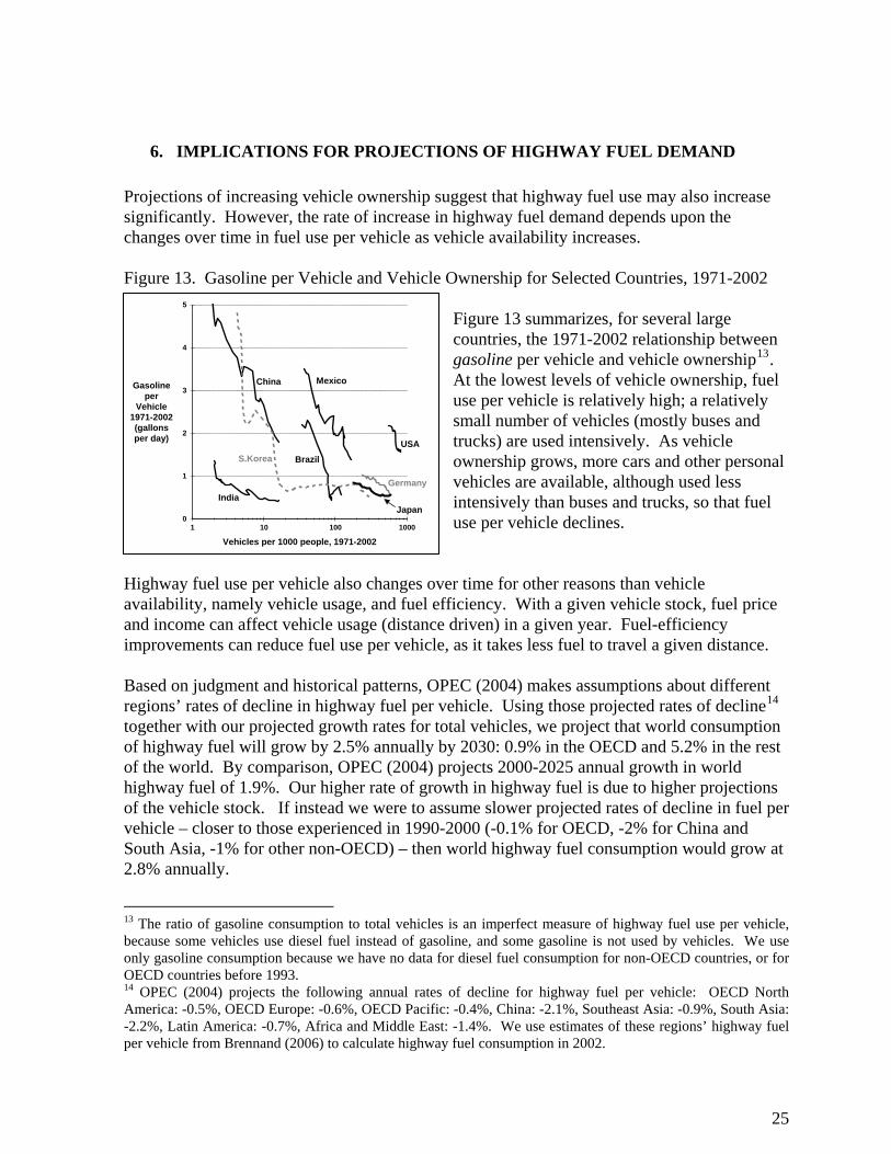
6. IMPLICATIONS FOR PROJECTIONS OF HIGHWAY FUEL DEMAND Projections of increasing vehicle ownership suggest that highway fuel use may also increase significantly. However, the rate of increase in highway fuel demand depends upon the changes over time in fuel use per vehicle as vehicle availability increases. Figure 13. Gasoline per Vehicle and Vehicle Ownership for Selected Countries, 1971-2002

Figure 13 summarizes, for several large countries, the 1971-2002 relationship between gasoline per vehicle and vehicle ownership13. At the lowest levels of vehicle ownership, fuel use per vehicle is relatively high; a relatively small number of vehicles (mostly buses and trucks) are used intensively. As vehicle ownership grows, more cars and other personal vehicles are available, although used less intensively than buses and trucks, so that fuel use per vehicle declines.

Highway fuel use per vehicle also changes over time for other reasons than vehicle availability, namely vehicle usage, and fuel efficiency. With a given vehicle stock, fuel price and income can affect vehicle usage (distance driven) in a given year. Fuel-efficiency improvements can reduce fuel use per vehicle, as it takes less fuel to travel a given distance. Based on judgment and historical patterns, OPEC (2004) makes assumptions about different regions’ rates of decline in highway fuel per vehicle. Using those projected rates of decline14 together with our projected growth rates for total vehicles, we project that world consumption of highway fuel will grow by 2.5% annually by 2030: 0.9% in the OECD and 5.2% in the rest of the world. By comparison, OPEC (2004) projects 2000-2025 annual growth in world highway fuel of 1.9%. Our higher rate of growth in highway fuel is due to higher projections of the vehicle stock. If instead we were to assume slower projected rates of decline in fuel per vehicle – closer to those experienced in 1990-2000 (-0.1% for OECD, -2% for China and South Asia, -1% for other non-OECD) – then world highway fuel consumption would grow at 2.8% annually.

13 The ratio of gasoline consumption to total vehicles is an imperfect measure of highway fuel use per vehicle, because some vehicles use diesel fuel instead of gasoline, and some gasoline is not used by vehicles. We use only gasoline consumption because we have no data for diesel fuel consumption for non-OECD countries, or for OECD countries before 1993. 14 OPEC (2004) projects the following annual rates of decline for highway fuel per vehicle: OECD North America: -0.5%, OECD Europe: -0.6%, OECD Pacific: -0.4%, China: -2.1%, Southeast Asia: -0.9%, South Asia: -2.2%, Latin America: -0.7%, Africa and Middle East: -1.4%. We use estimates of these regions’ highway fuel per vehicle from Brennand (2006) to calculate highway fuel consumption in 2002.

25

7. CONCLUSIONS We use a comprehensive data set covering 45 countries over 1960-2002 to explain historical patterns in the vehicle ownership rates as an S-shaped, Gompertz function of per-capita income. Our model specification exploits the similarity of response in vehicle ownership rates to per-capita income across countries over time, while allowing for cross-country variation in the speed of vehicle ownership growth and in ownership saturation levels. The relationship between vehicle ownership and per-capita income is highly non-linear. The income elasticity of vehicle ownership starts low but increases rapidly over the range of $3,000 to $10,000, when vehicle ownership increases twice as fast as per-capita income. Europe and Japan were at this stage in the 1960’s. Many developing countries, especially in Asia, are currently experiencing similar developments and will continue to do so during the next two decades. When income levels increase to the range of $10,000 to $20,000, vehicle ownership increases only as fast as income. At very high levels of income, vehicle ownership growth decelerates and slowly approaches the saturation level. Most of the OECD countries are at this stage now. We project that the world’s total vehicle stock will be 2.5 times greater in 2030 than in 2002, increasing to more than two billion vehicles. Non-OECD countries’ share of total vehicles will rise from 24% to 56%, as they acquire over three-fourths of the additional vehicles. China’s vehicle stock will increase nearly twenty-fold, to 390 million by 2030 – more vehicles than the USA – even though its rate of vehicle ownership (about 270 vehicles per 1000 people) will be only at levels experienced by Japan and Western Europe in the mid-1970’s, and by South Korea in 2001. As in most countries, vehicle ownership in China, India, Indonesia and elsewhere will grow twice as rapidly as its per-capita income, as these countries pass through middle-income levels of $3,000 to $10,000 per capita. By 2030, vehicle ownership in virtually all the OECD countries will have reached saturation, but in most of Asia it will still only be at 15% to 45% of ownership saturation levels. Finally, our results suggest that the future strong growth in the vehicle stock in developing countries will lead to significant increases in oil demand from the transport sector. We project annual worldwide growth in highway fuel demand to be in the range of 2.5% to 2.8%. ACKNOWLEDGEMENTS The authors wish to thank Karl Storchmann for helpful suggestions. Paul Atang, Stephanie Denis, and Angela Espiritu provided excellent research assistance.

26

REFERENCES Button K, Ngoe N, Hine J.

Modeling Vehicle Ownership and Use in Low Income Countries. Journal of Transport Economics and Policy. January 1983. p. 51-67.

Brennand G. Transportation sector modeling at the OPEC Secretariat. Workshop on Fuel Demand Modeling in the Transportation Sector. Vienna. 20th January; 2006.

Dargay J. The effect of income on car ownership: evidence of asymmetry. Transportation Research. 2001; Part A, 35. p. 807-821.

Dargay J, Gately D. Income's effect on car and vehicle ownership, worldwide: 1960-2015. Transportation Research, 1999; Part A, 33. p. 101-138.

Exxon Mobil. 2005 Energy Outlook. December 2005. http://www.exxonmobil.com/Corporate/Citizenship/Imports/ EnergyOutlook05/2005_energy_outlook.pdf

International Energy Agency (IEA). World Energy Outlook 2004. International Energy Agency. Paris. -----, World Energy Outlook 2005.

International Energy Agency. Paris. Mogridge MJH.

The Car Market: A Study of the Statics and Dynamics of Supply-Demand Equilibrium. London: Pion. 1983.

-----, The prediction of car ownership and use revisited - The beginning of the end? Journal of Transport Economics and Policy. 1989; XIII (1). p. 55-74.

Organization of the Petroleum Exporting Countries (OPEC). Oil Outlook to 2025. OPEC Review paper. September 2004.

Storchmann K. Long-run Gasoline Demand for Passenger Cars: The role of income distribution. Energy Economics. 2005; January; 27 (1). p. 25-58.

27

APPENDIX A: Data Sources This appendix provides further details on the datasets used in the analysis of vehicle ownership. Vehicle ownership data are primarily from the United Nations Statistical Yearbook. The data for a few country-years are from the national statistical offices. Historical data on Purchasing-Power-Parity (PPP) adjusted gross domestic product are from the OECD’s SourceOECD database. The data are expressed in thousands of 1995 PPP-adjusted dollars. Where necessary, the series were spliced with real GDP data from IMF’s World Economic Outlook database using the assumption that growth in the PPP GDP rate equals real GDP growth. Data on the real GDP growth projections for 2005-09 are from the IMF’s World Economic Outlook. For 2010-30, the main data source is the U.S. Department of Energy (DoE) International Energy Outlook April 2004. An adjustment was made to the DoE’s growth projection for China and India. In both cases, the long-term growth rates were reduced by 1 percentage point (specifically for China, the growth rate is 5 percent annually over 2010-14, 4.4 percent over 2015-2019, and 4.1 percent over 2020-2030; for India, the growth rate assumption is 4.3 during 2010-2014, 4.1 percent during 2015-2019, and 3.9 during 2020-2030). This adjustment was made to reduce the PPP-weighted world growth rate to its historical average of about 3.5 percent a year. This adjustment may create a downward bias in our vehicles projection if, in the future, world GDP growth will turn out to be higher than the historical average. The data on urbanization and land area are from the World Bank’s World Development Indicators database. Urbanization is expressed in percentage points and land area is expressed in square kilometers. The data on population, including projections, are from the United Nations database (median scenario). Population density was calculated by dividing total population by land area; it is measured by persons per square kilometer.

28