Vectors and Tensors - IIT Hyderabadashok/Maths_Lectures/TutorialB/Vector_Tens… · Vectors and...
55
1 Vectors and Tensors The mechanics of solids is a story told in the language of vectors and tensors. These abstract mathematical objects provide the basic building blocks of our analysis of the behavior of solid bodies as they deform and resist force. Anyone who stands poised to undertake the study of structural mechanics has undoubt- edly encountered vectors at some point. However, in an effort to establish a least common denominator among readers, we shall do a quick review of vec- tors and how they operate. This review serves the auxiliary purpose of setting up some of the notational conventions that will be used throughout the book. Our study of mechanics will naturally lead us to the concept of the tensor, which is a subject that may be less familiar (possibly completely unknown) to the reader who has the expected background knowledge in elementary me- chanics of materials. We shall build the idea of the tensor from the ground up in this chapter with the intent of developing a facility for tensor operations equal to the facility that most readers will already have for vector operations. In this book we shall be content to stick with a Cartesian view of tensors in rec- tangular coordinate systems. General tensor analysis is a mathematical subject with great beauty and deep significance. However, the novice can be blinded by its beauty to the point of missing the simple physical principles that are the true subject of mechanics. So we shall cling to the simplest possible rendition of the story that still respects the tensorial nature of solid mechanics. Mathematics is the natural language of mechanics. This chapter presents a fairly brief treatment of the mathematics we need to start our exploration of solid mechanics. In particular, it covers some basic algebra and calculus of vectors and tensors. Plenty more math awaits us in our study of structural me-
Transcript of Vectors and Tensors - IIT Hyderabadashok/Maths_Lectures/TutorialB/Vector_Tens… · Vectors and...
1 Vectors and Tensors
The mechanics of solids is a story told in the language of vectors and tensors. These abstract mathematical objects provide the basic building blocks of our analysis of the behavior of solid bodies as they deform and resist force. Anyone who stands poised to undertake the study of structural mechanics has undoubtedly encountered vectors at some point. However, in an effort to establish a least common denominator among readers, we shall do a quick review of vectors and how they operate. This review serves the auxiliary purpose of setting up some of the notational conventions that will be used throughout the book.
Our study of mechanics will naturally lead us to the concept of the tensor, which is a subject that may be less familiar (possibly completely unknown) to the reader who has the expected background knowledge in elementary mechanics of materials. We shall build the idea of the tensor from the ground up in this chapter with the intent of developing a facility for tensor operations equal to the facility that most readers will already have for vector operations. In this book we shall be content to stick with a Cartesian view of tensors in rectangular coordinate systems. General tensor analysis is a mathematical subject with great beauty and deep significance. However, the novice can be blinded by its beauty to the point of missing the simple physical principles that are the true subject of mechanics. So we shall cling to the simplest possible rendition of the story that still respects the tensorial nature of solid mechanics.
Mathematics is the natural language of mechanics. This chapter presents a fairly brief treatment of the mathematics we need to start our exploration of solid mechanics. In particular, it covers some basic algebra and calculus of vectors and tensors. Plenty more math awaits us in our study of structural me-
2 Fundamentals of Structural Mechanics
chanics, but the rest of the math we will develop on the fly as we need it, complete with physical context and motivation.
This chapter lays the foundation of the mathematical notation that we will use throughout the book. As such, it is both a starting place and a refuge to regain one's footing when the going gets tough.
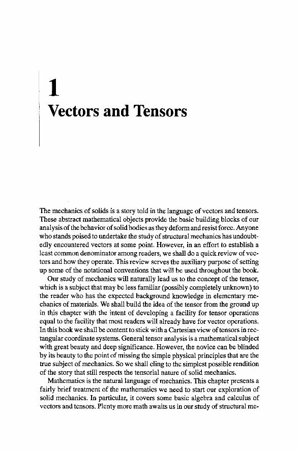
The Geometry of Three-dimensional Space We live in three-dimensional space, and all physical objects that we are familiar with have a three-dimensional nature to their geometry. In addition to solid bodies, there are basically three primitive geometric objects in three-dimensional space: the point, the curve, and the surface. Figure 1 illustrates these objects by taking a slice through the three-dimensional solid body 98 (a cube, in this case). A point describes position in space, and has no dimension or size. The point 9 in the figure is an example. The most convenient way to describe the location of a point is with a coordinate system like the one shown in the figure. A coordinate system has an origin 0 (a point whose location we understand in a deeper sense than any other point in space) and a set of three coordinate durections that we use to measure distance. Here we shall confine our attention to Cartesian coordinates, wherein the coordinate directions are mutually perpendicular. The location of a point is then given by its coordinates x = (jCi, JC2, JC3). A point has a location independent of any particular coordinate system. The coordinate system is generally introduced for the convenience of description or numerical computation.
A curve is a one-dimensional geometric object whose size is characterized by its arc length. In a sense, a curve can be viewed as a sequence of points. A curve has some other interestmg properties. At each point along a curve, the curve seems to be heading in a certain direction. Thus, a curve has an orientation in space that can be characterized at any point along the curve by the line tangent to the curve at that point. Another property of a curve is the rate at which this orientation changes as we move along the curve. A straight line is
Figure 1 The elements of the geometry of three-dimensional space
Chapter 1 Vectors and Tensors 3
a curve whose orientation never changes. The curve C exemplifies the geometric notion of curves in space.
A surface is a two-dimensional geometric object whose size is characterized by its surface area. In a certain sense, a surface can be viewed as a family of curves. For example, the collection of lines parallel and perpendicular to the curve e constitute a family of curves that characterize the surface ^. A surface can also be viewed as a collection of points. Like a curve, a surface also has properties related to its orientation and the rate of change of this orientation as we move to adjacent points on the surface. The orientation of a surface is completely characterized by the single line that is perpendicular to the tangent lines of all curves that pass through a particular point. This line is called the normal direction to the surface at the point. A flat surface is usually called a plane, and is a surface whose orientation is constant.
A three-dimensional solid body is a collection of points. At each point, we ascribe some physical properties (e.g., mass density, elasticity, and heat capacity) to the body. The mathematical laws that describe how these physical properties affect the interaction of the body with the forces of nature summarize our understanding of the behavior of that body. The heart of the concept of continuum mechanics is that the body is continuous, that is, there are no finite gaps between points. Clearly, this idealization is at odds with particle physics, but, in the main, it leads to a workable and useful model of how solids behave. The primary purpose of hanging our whole theory on the concept of the continuum is that it allows us to do calculus without worrying about the details of material constitution as we pass to infinitesimal limits. We will sometimes find it useful to think of a solid body as a collection of lines, or a collection of surfaces, since each of these geometric concepts builds from the notion of a point in space.
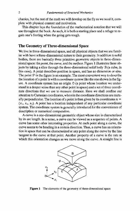
Vectors A vector is a directed line segment and provides one of the most useful geometric constructs in mechanics. A vector can be used for a variety of purposes. For example, in Fig. 2 the vector v records the position of point b relative to point a. We often refer to such a vector as 2i position vector, particularly when a is the origin of coordinates. Qose relatives of the position vector are displacement (the difference between the position vectors of some point at different times), velocity (the rate of change of displacement), znd acceleration (the rate of change of velocity). The other common use of the notion of a vector, to which we shall appeal in this book, is the concept oi force. We generally think
Figure 2 A vector is a directed line segment

4 Fundamentals of Structural Mechanics
offeree as an action that has a magnitude and a direction. Likewise, displacements are completely characterized by their magnitude and direction. Because a vector possesses only the properties of magnitude (length of the line) and direction (orientation of the line in space), it is perfectly suited to the mathematical modeling of things like forces and displacements. Vectors have many other uses, but these two are the most important in the present context.
Graphically, we represent a vector as an arrow. The shaft of the arrow gives the orientation and the head of the arrow distinguishes the direction of the vector from the two possibilities inherent in the line segment that describes the shaft (i.e., line segments ab and ba in Fig. 2 are both oriented the same way in space). The length, or magnitude, of a vector v is represented graphically by the length of the shaft of the arrow and will be denoted symbolically as || v || throughout the book.
The magnitude and direction of a vector do not depend upon any coordinate system. However, for computation it is most convenient to describe a vector in relation to a coordinate system. For that purpose, we endow our coordinate system with unit base vectors {Ci, 62, €3} pointing in the direction of the coordinate axes. The base vectors are geometric primitives that are introduced purely for the purpose of establishing the notion of direction. Like the origin of coordinates, we view the base vectors as vectors that we understand more deeply and intuitively than any other vector in space. Basically, we assume that we know what it means to be pointing in the Ci direction, for example. Any collection of three vectors that point in different directions makes a suitable basis (in the language of linear algebra we would say that three such vectors span three-dimensional space). Because we have introduced the notion of base vectors for convenience, we shall adopt the most convenient choice. Throughout this book, we will generally employ orthogonal unit vectors in conjunction with a Cartesian coordinate system.
Any vector can be described in terms of its components relative to a set of base vectors. A vector v can be written m terms of base vectors {ci, €2, €3) as
V = Viei + V2e2 + V3e3 (1)
where Vj, V2, and V3 are called the components of the vector relative to the basis. The component v, measures how far the vector extends in the e, direction, as shown in Fig. 3. A component of a vector is a scalar.
Vector operations. An abstract mathematical construct is not really useful until you know how to operate with it. The most elementary operations in mathematics are addition and multiplication. We know how to do these operations for scalars; we must establish some corresponding operations for vectors.
Vector addition is accomplished with the head-to-tail rule or parallelogram rule. The sum of two vectors u and v, which we denote u H- v, is the vector connecting the tail of u with the head of v when the tail of v lies at the head of u, as shown in Fig. 4. If the vectors u and v are replicated to form the sides of a

Chapter 1 Vectors and Tensors
•=3 i
Figure 3 The components of a vector relative to a basis
parallelogram abed, then u + v is the diagonal ac of the parallelogram. Subtraction of vectors can be accomplished by introducing the negative of a vector, — V (segment bf in Fig. 4), as a vector with the same magnitude that points in exactly the opposite direction of v. Then, u - v is simply realized as u + ( - v). If we construct another parallelogram abfe, then u — v is the diagonal af. It is evident from the figure that segment af is identical in length and direction to segment db, A vector can be added to another vector, but a vector and a scalar cannot be added (the well-worn analogy of the impossibility of adding apples and oranges applies here).
We can multiply a vector v by a scalar a to get a vector a\ having the same direction but a length equal to the original length || v || multiplied by a. If the scalar a has a negative value, then the sense of the vector is reversed (i.e., it puts the arrow head on the other end). With these definitions, we can make sense of Eqn. (1). The components v, multiply the base vectors C/to give three new vectors VjCi, V2e2, and v^e^. The resulting vectors are added together by the head-to-tail rule to give the final vector v.
The operation of multiplication of two vectors, say u and v, comes in three varieties: The dot product (often called the scalar product) is denoted u • v; the cross product (often called the vector product) is denoted u x v; and the tensor product is denoted u (8) v. Each of these products has its own physical significance. In the following sections we review the definitions of these terms, and examine the meaning behind carrying out such operations.
Figure 4 Vector addition and subtraction by the head-to-tail or parallelogram rule

Fundamentals of Structural Mechanics
v - u
Figure 5 The angle between two vectors
The dot product. The dot product is a scalar value that is related to not only the lengths of the vectors, but also the angle between them. In fact, the dot product can be defined through the formula
u • V = II u IIII V II COS 9(u, v) (2)
where cos0(u, v) is the cosine of the angle 0 between the vectors u and v, shown in Fig. 5. The definition of the dot product can be expressed directly in terms of the vectors u and v by using the law of cosines, which states that
II u p + II V p = II v - u P + 2 II u IIII v II cose(u, V)
Using this result to eliminate 6 from Eqn. (2), we obtain the equivalent definition of the dot product
v = + iivr-iiv-ur) (3)
We can think of the dot product as measuring the relative orientation between two vectors. The dot product gives us a means of defining orthogonality of two vectors. Two vectors are orthogonal if they have an angle of jr/2 radians between them. According to Eqn. (2), any two nonzero vectors u and v are orthogonal if u • V = 0. If u and V are orthogonal, then they are the legs of a right triangle with the vector v — u forming the hypotenuse. In this case, we can see that the Pythagorean theorem makes the right-hand side of Eqn. (3) equal to zero. Thus, u • v = 0, as before.
Equation (3) suggests a means of computing the length of a vector. The dot product of a vector v with itself is v • v = || v p. With this observation Eqn. (2) verifies that the cosine of zero (the angle between a vector and itself) is one.
The dot product is commutative, that is, u • v = v • u. The dot product also satisfies the distributive law. In particular, for any three vectors u, v, and w and scalars a, fi, and y, we have
an ' (^v-hyw) = afi(u • v) + ay(n • w) (4)
The dot product can be computed from the components of the vectors as 3 3 3 3
; = i / = 1 ; = 1
Chapter 1 Vectors and Tensors 7
In the first step we merely rewrote the vectors u and v in component form. In the second step we simply distributed the sums. If the last step puzzles you then you should write out the sums in longhand to demonstrate that the mathematical maneuver was legal. Because the base vectors are orthogonal and of unit length, the products e, • e are all either zero or one. Hence, the component form of the dot product reduces to the expression
u • V (5)
The dot product of the base vectors arises so frequently that it is worth introducing a shorthand notation. Let the symbol dij be defined such that
1 0 if / 7 ; (6)
The symbol 5y is often referred to as the Kronecker delta, Qearly, we can write ti • Cy = diy When the Kronecker delta appears in a double summation, that part of the summation can be carried out explicitly (even without knowing the values of the other quantities involved in the sum!). This operation has the effect of contraction from a double sum to a single summation, as follows
3 3 3
1 = 1 ; = 1 / = 1
A simple way to see how this contraction comes about is to write out the sum of nine terms and observe that six of them are multiplied by zero because of the definition of the Kronecker delta. The remaining three terms always share a common value of the indices and can, therefore, be written as a single sum, as indicated above.
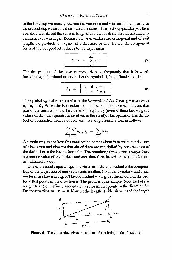
One of the most important geometric uses of the dot product is the computation of the projection of one vector onto another. Consider a vector v and a unit vector n, as shown in Fig. 6. The dot product v • n gives the amount of the vector V that points in the direction n. The proof is quite simple. Note that ahc is a right triangle. Define a second unit vector m that points in the direction be. By construction m • n = 0. Now let the length of side ab be y and the length
Figure 6 The dot product gives the amount of v pointing in the direction n
8 Fundamentals of Structural Mechanics
of side fee be j8. The vector ab is then y n and the vector be is j3 m. By the head-to-tail rule we have v = yn+)Sm. Taking the dot product of both sides of this expression with n we arrive at the result
V • n = (yn-hjSm) - n = y
since n • n = 1. But y is the length of the side ab, proving the original assertion. This observation can be used to show that the dot product of a vector with one of the base vectors has the effect of picking out the component of the vector associated with the base vector used in the dot product. To wit,
3 3
1 = 1 J = l
We can summarize the geometric significance of the vector components as
= e„ (8)
That is, v^ is the amount of v pointing in the direction e,^^
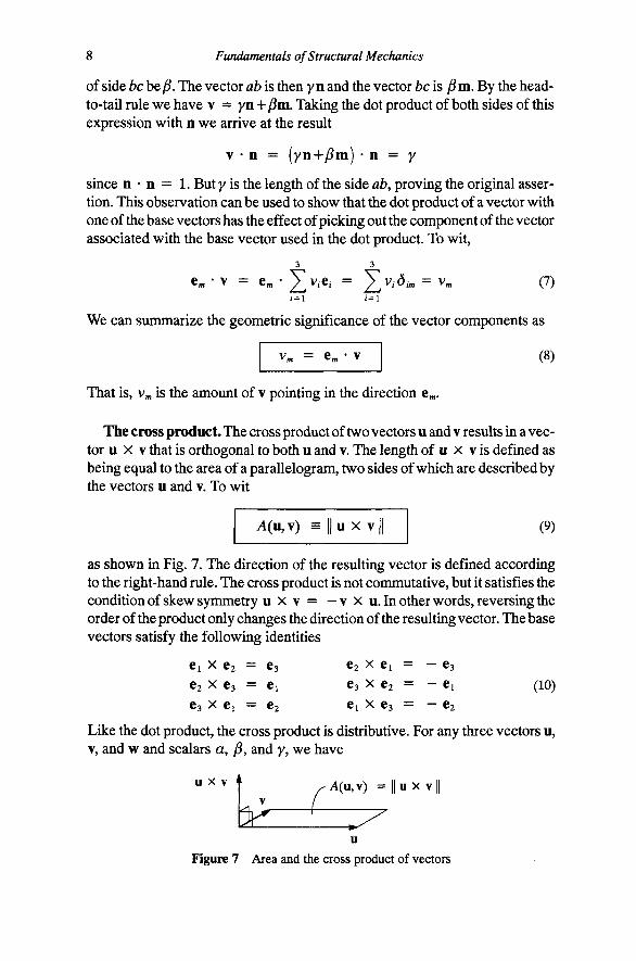
The cross product. The cross product of two vectors u and v results in a vector u x v that is orthogonal to both u and v. The length of u x v is defined as being equal to the area of a parallelogram, two sides of which are described by the vectors u and v. To wit
A(u,v) = ||u X vl (9)
as shown in Fig. 7. The direction of the resulting vector is defined according to the right-hand rule. The cross product is not commutative, but it satisfies the condition of skew symmetry u x v = — v x u. In other words, reversing the order of the product only changes the direction of the resulting vector. The base vectors satisfy the following identities
Ci X 62 = Ca
€2 X ©3 = Cj
©3 X Cj ^ ©2
©2 X Cj — ©3
63 X 62 = - Ci
Ci X 63 = - 62
(10)
Like the dot product, the cross product is distributive. For any three vectors u, V, and w and scalars a, ^, and y, we have
U X V •
^ ^ I A(u,v) = | |ux v|
Figure 7 Area and the cross product of vectors
Chapter 1 Vectors and Tensors
an X (^v+yw) = a^(u x v) + ay(u x w)
The component form of the cross product of vectors u and v is
3 3 3 3
u x v = J^M.e,- xj^v^-e,- = X Z" ' ' ' > (^ ' ^ ^ l
9
(11)
) = i / = 1 ; = 1
where, again, we have first represented the vectors in component form and then distributed the product. Carrying out the summations, substituting the appropriate incidences of Eqn. (10) for each term of the sum, the component form of the cross product reduces to the expression
U X V = ( M 2 ^ 3 ~ W 3 ^ 2 ) C I + (W3VI—WiV3)e2 + (WiV2~W2^l)C3 (12)
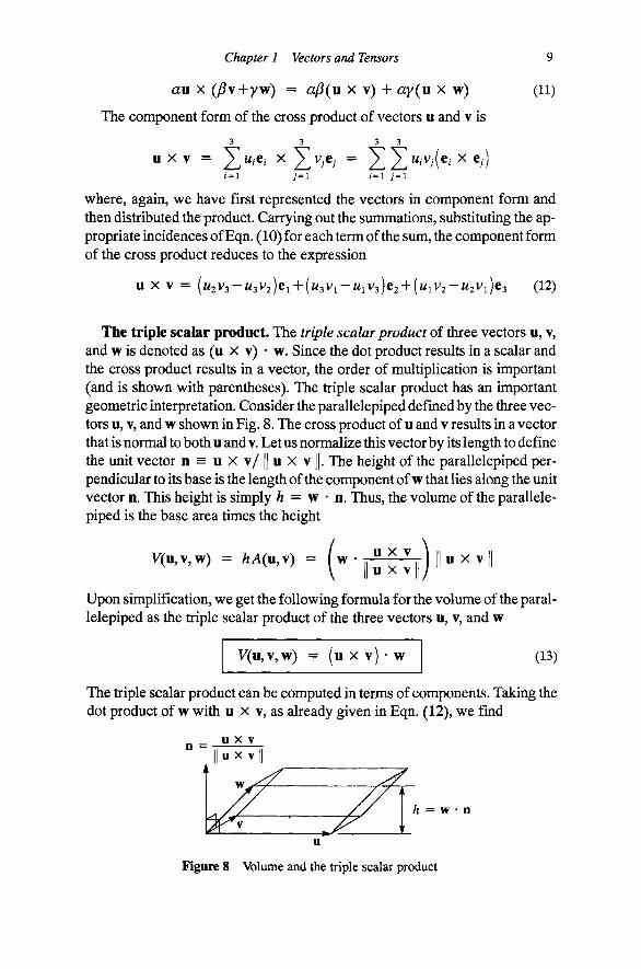
The triple scalar product. The triple scalar product of three vectors u, v, and w is denoted as (u x v) • w. Since the dot product results in a scalar and the cross product results in a vector, the order of multiplication is important (and is shown with parentheses). The triple scalar product has an important geometric interpretation. Consider the parallelepiped defined by the three vectors u, V, and w shown in Fig. 8. The cross product of u and v results in a vector that is normal to both u and v. Let us normalize this vector by its length to define the unit vector n = u X v/ || u X v ||. The height of the parallelepiped perpendicular to its base is the length of the component of w that lies along the unit vector n. This height is simply A = w • n. Thus, the volume of the parallelepiped is the base area times the height
V(u,v,w) = AA(u,v) = ( w - u x v u X vl
u x v
Upon simplification, we get the following formula for the volume of the parallelepiped as the triple scalar product of the three vectors u, v, and w
V(u,v,w) = (u X v) • w (13)
The triple scalar product can be computed in terms of components. Taking the dot product of w with u x v, as already given in Eqn. (12), we find
n = u x v
/i = w • n
Figure 8 Volume and the triple scalar product
10 Fundamentals of Structural Medianics
(U X v ) • W = >Vi(w2V3""«3^2) + ^ 2 ( " 3 ^ 1 ~ " l ^ 3 ) + >^3(«1^2 ~ "2 ^1)
= (WiV2W3 + M2V3> l + " 3 ^ 1 ^ 2 ) ~ (W3V2IV1 + W2^1^3 + " l ^ 3 ^ 2 )
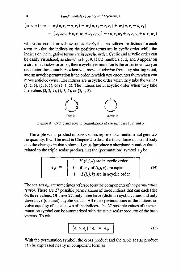
where the second form shows quite clearly that the indices are distinct for each term and that the indices on the positive terms are in cyclic order while the indices on the negative terms are in acyclic order. Cyclic and acyclic order can be easily visualized, as shown in Fig. 9. If the numbers 1, 2, and 3 appear on a circle in clockwise order, then a cyclic permutation is the order in which you encounter these numbers when you move clockwise from any starting point, and an acyclic permutation is the order in which you encounter them when you move anticlockwise. The indices are in cyclic order when they take the values (1, 2, 3), (2, 3,1), or (3,1, 2). The indices are in acyclic order when they take the values (3, 2, l), (l, 3, 2), or (2, l, 3).
r'\ <'>.
Cyclic Acyclic
Figure 9 Cyclic and acyclic permutations of the numbers 1, 2, and 3
The triple scalar product of base vectors represents a fundamental geometric quantity. It will be used in Chapter 2 to describe the volume of a solid body and the changes in that volume. Let us introduce a shorthand notation that is related to the triple scalar product. Let the (permutation) symbol e tbe
(14)
The scalars eijk are sometimes referred to as the components of thopermutation tensor. There are 27 possible permutations of three indices that can each take on three values. Of these 27, only three have (distinct) cyclic values and only three have (distinct) acyclic values. All other permutations of the indices involve equality of at least two of the indices. The 27 possible values of the permutation symbol can be summarized with the triple scalar products of the base vectors. To wit.
eijk = <
' 1 if (/,;, k) are in cyclic order
0 if any of (/,;, k) are equal
^ - 1 if (/,;, k) are in acyclic order
(e,- X e,.) • e* = e,yt (15)
With the permutation symbol, the cross product and the triple scalar product can be expressed neatly in component form as
Chapter 1 Vectors and Tensors 11
3 3 3
1=1 j = l i t= l
3 3 3
(ux v)-w = XZZ"'''^'^^^^-*
1 = 1 , = 1 i t = l
3 3 3 (16)
1 = 1 ; = 1 i t = l
You should verify that these formulas involving e^k give the same results as found previously.
Tensors The cross product is an example of a vector operation that has as its outcome a new vector. It is a very special operator in the sense that it produces a vector orthogonal to the plane containing the two original vectors. There is a much broader class of operations that produce vectors as the result. The second-order tensor is the mathematical object that provides the appropriate generalization. (If the context is not ambiguous, we will often refer to a second-order tensor simply as a tensor.)
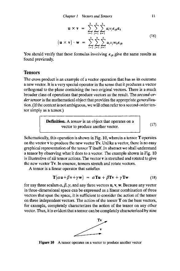
Definition. A tensor is an object that operates on a vector to produce another vector. (17)
Schematically, this operation is shown in Fig. 10, wherein a tensor T operates on the vector v to produce the new vector Tv. Unlike a vector, there is no easy graphical representation of the tensor T itself. In abstract we shall understand a tensor by observing what it does to a vector. The example shown in Fig. 10 is illustrative of all tensor actions. The vector v is stretched and rotated to give the new vector Tv. In essence, tensors stretch and rotate vectors.
A tensor is a linear operator that satisfies
T(au+)8v+yw) = aTu + )8Tv + yTw (18)
for any three scalars a,)8, y, and any three vectors u, v, w. Because any vector in three-dimensional space can be expressed as a linear combination of three vectors that span the space, it is sufficient to consider the action of the tensor on three independent vectors. The action of the tensor T on the base vectors, for example, completely characterizes the action of the tensor on any other vector. Thus, it is evident that a tensor can be completely characterized by nme
Figure 10 A tensor operates on a vector to produce another vector
12 Fundamentals of Structural Mechanics
scalar quantities: the three components of the vector Tci, the three components of the vector Te2, and the three components of the vector Tcs. We shall refer to these nine scalar quantities as the components of the tensor. Like a vector, which can be expressed as the sum of scalar components times base vectors, we shall represent a tensor as the sum of scalar components times base tensors. We introduce the tensor product of vectors as the building block to define a natural basis for a second-order tensor.
The tensor product of vectors. The tensor product of two vectors u and v is a special second-order tensor which we shall denote [u ® v]. The action of this tensor is embodied in how it operates on a vector w, which is
[u 0 v]w = (v • w)u (19)
In other words, when the tensor u (8) v operates on w the result is a vector that points in the direction u and has the length equal to (v • w) || u ||, the original length of u multiplied by the scalar product of v and w. The tensor product of vectors appears to be a rather curious object, and it certainly takes some getting used to. It will, however, prove to be highly useful in developing a coordinate representation of a general tensor T.
The tensor products of the base vectors e, (8) e comprise a set of second-order tensors. Since there are three base vectors, there are nine distinct tensor product combinations among them. These nine tensors provide a suitable basis for expressing the components of a tensor, much like the base vectors themselves provided a basis for expressing the components of a vector. Like the base vectors, we presume to understand these base tensors better than any other tensors in the space. We can confirm that by noting that their action is given simply by Eqn. (19). In fact, we can observe from Eqn. (19) that
[e,(8)e,]e;t = (ey-e^tje,- = dj^ti (20)
We will use this knowledge of the tensor product of base vectors to help us with the manipulation of tensor components.
The second-order tensor T can be expressed in terms of its components T relative to the base tensors e, (S) e as
^ = a^^le^^ej] (21)
It will soon be evident why we elect to represent the nine scalar components with a double indexed quantity. Like vector components, the components T are scalar values that depend upon the basis chosen for the representation. The tensor part of T comes from the base tensors e, 0 e . The tensor, then, is a sum of scalars times base tensors. Like a vector, the tensor T itself does not depend upon the coordinate system; only the components do.
Chapter 1 Vectors and Tensors 13
A tensor is completely characterized by its action on the three base vectors. Let us compute the action of T on the base vector e ,
3 3 3 3 3
t = l J = l i = l ; = 1
The first step simply introduces the coordinate form of T. The second step carries out the tensor product of vectors as in Eqn. (20). The final step recognizes that the sum of nine terms reduces to a sum of three terms because six of the nine terms are equal to zero.
We can get some insight into the physical significance of the components by taking the dot product of e^ andXe^. Recall from Eqn. (8) that dotting a vector with e^ simply extracts the wth component of the vector. Starting from the result of Eqn. (22) we compute
(23)
Thus, we can see that r^„ is the wth component of the vector Te„. We can summarize the physical significance of the tensor components as follows
T = e • Te (24)
The identity tensor. The identity tensor is the tensor that has the property of leaving a vector unchanged. We shall denote the identity tensor as I, and endow it with the property that Iv = v, for all vectors v. The identity tensor can be expressed in terms of orthonormal (i.e., orthogonal and unit) base vectors
I = X*'®®' (25)
Of course, this definition holds for any orthonormal basis. To prove that Eqn. (25), we need only consider the action of I on a base vector Cy. To wit
3 3 3
/ = 1 1 = 1 1 = 1
Since the base vectors span three-dimensional space, it is apparent that Iv = v for any vector. Observe that Eqn. (25) can br expressed in terms of the Kro-necker delta as
I = EZ^'>[*'®«>] . = 1 ) = i

14 Fundamentals of Structural Mechanics
Hence, 6y can be interpreted as the yth component of the identity tensor.
The tensor inverse. Let us assume that we have a tensor T and that it acts on a vector v to produce another vector Tv. A tensor stretches and rotates a vector. It seems reasonable to imagine a tensor that undoes the action of another tensor. Such a tensor is called the inverse of the tensor T, and we denote it as T~\ Thus, T"Ms the tensor that exactly undoes what the tensor T does. To be more specific, the tensor T"^ can be applied to the vector Tv to give back v. Conversely, if the tensor T ~ Ms applied to the vector v to give the vector T ~ v, then the tensor T can be applied to T " v to give back the vector v. These operations define the inverse of a tensor and are summarized as follows
T-i(Tv) = V, T(T-^v) = v (26)
The above relations hold for any vector v. As we will soon see, the composition of tensors (a tensor operating on a tensor) can be viewed as a tensor itself. Thus, we can say that T'^T = I and TT"^ = I.
Example 1. As a simple example of a tensor and its operation on vectors, consider tht projection tensor P that generates the image of a vector v projected onto the plane with normal n, as shown in Fig. 11.
Figure 11 The action of the projection tensor
The explicit expression for the tensor is given by
P = I - n ® n (27)
where I is the identity tensor. The action of P on v gives the result
Pv = [l-n(8)n]v
= Iv - [n® n]v
= V - (n • v)n
To see that the vector Pv lies in the plane we need only to show that its dot product with the normal vector n is zero. Accordingly, we can make the computation Pv • n = (v • n)-(v • n)(n • n) = 0, since n is a unit vector.
It is interesting to note that we can derive the tensor P from geometric considerations. From Fig. 11 we can see that, by vector addition, Pv+j8n = v for some, as yet unknown, value of the scalar^. To determiners we simply take the dot product of the previous vector equation with the vector n, noting that n has unit length and is perpendicular to Pv. Hence, )3 = v • a Now, we substitute back to get
Chapter 1 Vectors and Tensors 15
Pv = v - i 8 n = V - (v • n)n = [ l - n ® n ] v (28)
thereby determining the tensor P.
Component expression for operation of a tensor on a vector. Equipped with the component representation of a tensor we can now take another look at how a tensor T operates on a vector v. In particular, let us examine the components of the resulting vector Tv.
3 3 3 3 3 3
1=1 j = l k=\ i=l ; = 1 k=\
Carrying out the summations in Eqn. (29), noting the properties expressed in Eqn. (20), we finally obtain the result
3 3
/ = i y = i
From this expression, we can see that the result is a vector (anything expressed in a vector basis is a vector). Furthermore, we can observe from Eqn. (30) that the ith component of the vector Tv is given by
3
(Tv), = X V ) (31)
That is, we compute the /th component of the resulting vector from the components of the tensor and the components of the original vector. The similarity between the operation of a tensor and that of a matrix in linear algebra should be apparent.
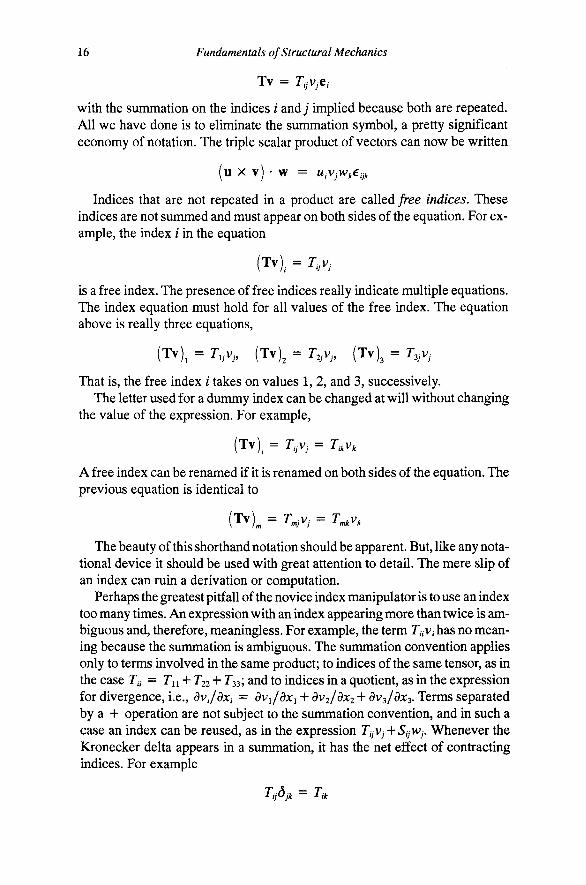
The summation convention. General relativity is a theory based on tensors. While Einstein was working on this theory, he apparently got rather tired of writing the summation symbol with its range of summation decorating the bottom and top of the Greek letter sigma. What he observed was that, most of the time, the range of the summation was equal to the dimension of space (three dimensions for us, four for him) and that when the summation involved a product of two terms, the summation was over a repeated index. For example, in Eqn. (31) the index; is the index of summation, and it appears exactly twice in the summand TijVj, Einstein decided that, with a little care, summations could be expressed without laboriously writing the summation symbol. The summation symbol would be understood to apply to repeated indices.
The summation convention, then,.means that any repeated index, also called a dummy index, is understood to be summed over the range 1 to 3. With the summation convention, then, Eqn. (30) can be written as
16 Fundamentals of Structural Mechanics
Tv = T^vje,
with the summation on the indices i and; implied because both are repeated. All we have done is to eliminate the summation symbol, a pretty significant economy of notation. The triple scalar product of vectors can now be written
(u X v) • w = UiVjWke^jk
Indices that are not repeated in a product are called free indices. These indices are not summed and must appear on both sides of the equation. For example, the index i in the equation
(Tv), = r,v,
is a free index. The presence of free indices really indicate multiple equations. The index equation must hold for all values of the free index. The equation above is really three equations,
(Tv), = V , , (Tv), = r,,v, (Tv)3 = r3,v,
That is, the free index i takes on values 1, 2, and 3, successively. The letter used for a dummy index can be changed at will without changing
the value of the expression. For example,
(Tv). = TijVj = r^v^
A free index can be renamed if it is renamed on both sides of the equation. The previous equation is identical to
(Tv)„ = T^jvj = r ^v ,
The beauty of this shorthand notation should be apparent. But, like any nota-tional device it should be used with great attention to detail. The mere slip of an index can ruin a derivation or computation.
Perhaps the greatest pitfall of the novice index manipulator is to use an index too many times. An expression with an index appearing more than twice is ambiguous and, therefore, meaningless. For example, the term r,7V,has no meaning because the summation is ambiguous. The summation convention applies only to terms involved in the same product; to indices of the same tensor, as in the case Ta = Tn + 722 + T^s; and to indices in a quotient, as in the expression for divergence, i.e., dvi/dxi = dv^/dxi + 3V2/6JC2 + dvs/dxs. Terms separated by a + operation are not subject to the summation convention, and in such a case an index can be reused, as in the expression TijVj + SijWj, Whenever the Kronecker delta appears in a summation, it has the net effect of contracting indices. For example
Chapter 1 Vectors and Tensors 17
Observe how the summed index ; on the tensor component Jy is simply replaced by the free index k on djk in the process of contraction of indices.
In this book the summation convention will be in force unless specifically indicated otherwise.
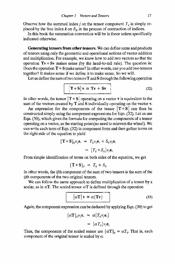
Generating tensors from other tensors. We can define sums and products of tensors using only the geometric and operational notions of vector addition and multiplication. For example, we know how to add two vectors so that the operation Tv + Sv makes sense (by the head-to-tail rule). The question is: Does the operation T + S make sense? In other words, can you add two tensors together? It makes sense if we define it to make sense. So we will.
Let us define the sum of two tensors T and S through the following operation
[T + S]v = Tv + Sv (32)
In other words, the tensor [ T + S] operating on a vector v is equivalent to the sum of the vectors created by T and S individually operating on the vector v.
An expression for the components of the tensor [T + S] can then be constructed simply using the component expressions for Eqn. (32). Let us use Eqn. (30), which gives the formula for computing the components of a tensor operating on a vector, as the starting point (no need to reinvent the wheel). We can write each term of Eqn. (32) in component form and then gather terms on the right side of the equation to yield
[T + S], v,e,- = V^e , + 5, v,.e,
= (r,+5,)v;e,
From simple identification of terms on both sides of the equation, we get
[T + S] . = r^ + 5,
In other words, the y th component of the sum of two tensors is the sum of the i/th components of the two original tensors.
We can follow the same approach to define multiplication of a tensor by a scalar, as in aT. The scaled tensor aT is defined through the operation
[aT]v = a(Tv) (33)
Again, the component expression can be deduced by applying Eqn. (30) to get
[aT], V;e,- = a(r^v,e,)
Thus, the components of the scaled tensor are [aT]y = aJy. That is, each component of the original tensor is scaled by a.
18 Fundamentals of Structural Mechanics
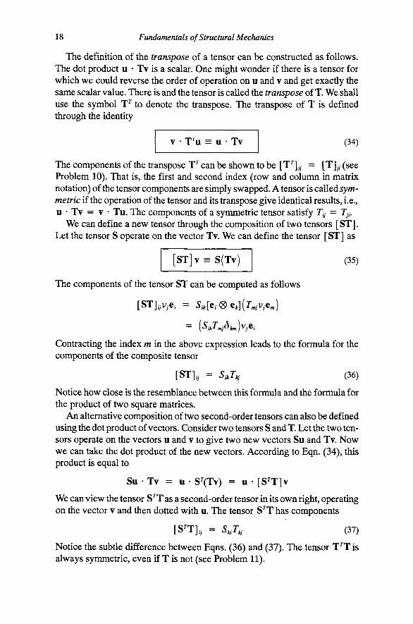
The definition of the transpose of a tensor can be constructed as follows. The dot product u • Tv is a scalar. One might wonder if there is a tensor for which we could reverse the order of operation on u and v and get exactly the same scalar value. There is and the tensor is called the transpose of T. We shall use the symbol T^ to denote the transpose. The transpose of T is defined through the identity
T^u = u • Tv (34)
The components of the transpose T^ can be shown to be [T^]y = [T]jj (see Problem 10). That is, the first and second index (row and column in matrix notation) of the tensor components are simply swapped. A tensor is called 5ym-metric if the operation of the tensor and its transpose give identical results, i.e., u • Tv = V • Tu. The components of a symmetric tensor satisfy Ty = Tji.
We can define a new tensor through the composition of two tensors [ST]. Let the tensor S operate on the vector Tv. We can define the tensor [ST] as
ST]v = S(Tv) (35)
The components of the tensor ST can be computed as follows
[ST],^v,e, = 5^[e,(8)ej(r,,v;e,)
Contracting the index m in the above expression leads to the formula for the components of the composite tensor
[ST]^ = Su^Tj^ (36)
Notice how close is the resemblance between this formula and the formula for the product of two square matrices.
An alternative composition of two second-order tensors can also be defined using the dot product of vectors. Consider two tensors S and T. Let the two tensors operate on the vectors u and v to give two new vectors Su and Tv. Now we can take the dot product of the new vectors. According to Eqn. (34), this product is equal to
Su Tv = u S^(Tv) = u [S^T]v
We can view the tensor S^T as a second-order tensor in its own right, operating on the vector v and then dotted with u. The tensor S^T has components
[S^T], = 5,T, (37)
Notice the subtle difference between Eqns. (36) and (37). The tensor T^T is always symmetric, even if T is not (see Problem 11).
Chapter 1 Vectors and Tensors 19
It should be clear that we could go on defining new tensor objects ad infinitum. Any such definition will emanate from the same basic considerations, and the computation of the components of the resulting tensors follows exactly along the lines given above. We shall have the opportunity to make such definitions throughout this book, and thus defer further discussion until needed.
Tensors, tensor components, and matrices. A tensor is not a matrix. However, if the foregoing discussion of tensors has left you thinking of matrices, you are not far off the mark. The way we have chosen to denote the components of a second-order tensor (with two indices, that is) makes the temptation to think of tensors as matrices quite compelling. We can list the components of a tensor in a matrix; all of the formulas for tensor-index manipulation are then exactly the same as standard matrix algebra. To some extent, matrix algebra can be an aid to understanding formulas like Eqn. (36). On the other hand, a second-order tensor is no more a three by three matrix than a vector is a three by one matrix.
Matrices are for keeping books, for organizing computations. A tensor or a vector exists independent of a particular manifestation of its components; a matrix is a particular manifestation of its components. So take the analogy between tensors and matrices for what it is worth, but try not to confuse a tensor with its components. To do so is rather like being unable to feel cold because you don't know the value of the temperature in degrees Celsius. The fundamental property of "cold" exists independent of what scale you choose to measure temperature.
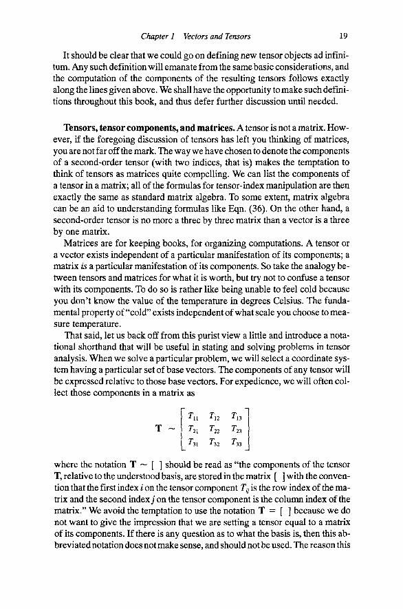
That said, let us back off from this purist view a little and introduce a nota-tional shorthand that will be useful in stating and solving problems in tensor analysis. When we solve a particular problem, we will select a coordinate system having a particular set of base vectors. The components of any tensor will be expressed relative to those base vectors. For expedience, we will often collect those components in a matrix as
T -
where the notation T ~ [ ] should be read as "the components of the tensor T, relative to the understood basis, are stored in the matrix [ ] with the convention that the first index / on the tensor component J^ is the row index of the matrix and the second index; on the tensor component is the column index of the matrix." We avoid the temptation to use the notation T = [ ] because we do not want to give the impression that we are setting a tensor equal to a matrix of its components. If there is any question as to what the basis is, then this abbreviated notation does not make sense, and should not be used. The reason this
Tn Tix
Tn
Tn
T22
T,2
Tn T23
Tyi
20 Fundamentals of Structural Mechanics
Ci v--- gi
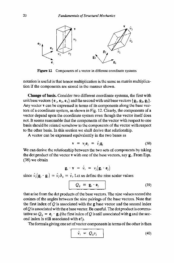
Figure 12 Components of a vector in different coordinate systems
notation is useful is that tensor multiplication is the same as matrix multiplication if the components are stored in the manner shown.
Change of basis. Consider two different coordinate systems, the first with unit base vectors {ei, €2, €3} andthe second with unit base vectors {gi, g2, gs}. Any vector v can be expressed in terms of its components along the base vectors of a coordinate system, as shown in Fig. 12. Qearly, the components of a vector depend upon the coordinate system even though the vector itself does not. It seems reasonable that the components of the vector with respect to one basis should be related somehow to the components of the vector with respect to the other basis. In this section we shall derive that relationship.
A vector can be expressed equivalently in the two bases as
V = vjej = vjgj (38)
We can derive the relationship between the two sets of components by taking the dot product of the vector v with one of the base vectors, say g,. From Eqn. (38) we obtain
g. . V = V, = v,.(g,. • e,)
since Vj[gj * g,) = Vjdij = v,. Let us define the nine scalar values
Qij = gi • C; (39)
that arise from the dot products of the base vectors. The nine values record the cosines of the angles between the nine pairings of the base vectors. Note that the first index of Q is associated with the g base vector and the second index of Q is associated with the e base vector. Be careful. The dot product is commutative so Qij = Cy • g, (the first index of Q is still associated with g and the second index is still associated with e!).
The formula giving one set of vector components in terms of the other is then
v/ = QijV^ (40)

Chapter 1 Vectors and Tensors 21
We can find the reverse relationship by dotting Eqn. (38) with e, instead of g . Carrying out a similar calculation we find that
V/ = QjiVj (41)
The components of a second-order tensor T transform in a manner similar to vectors. A tensor can be expressed in terms of components relative to two different bases in the following manner
T = Ug^^gj] = r ,[e,(8)ej
where Ty is the yth component of T with respect to the base tensor [g, (8) gj] and Tij is the yth component of T with respect to the base tensor [e, 0 e j . The relationship between the components in the two coordinate systems can be found by computing the product g^ • Tg;,, as follows
g, • Tg, = f^ = T,j(g^ ' e,)(g, • e,)
Computing instead e^ • Te , we can find the inverse relationship. Once again noting that j2// = g/ * Cy, we can write the formulas for the transformation of second-order tensor components as
- mn \lmi\lni ^ ij ^ mn SelimSdjn^ ij (42)
The main difference between transforming the components of a tensor and those of a vector is that it took two Q terms to accomplish the task for a tensor, one for each index, but only one Q term for a vector. It should be evident that higher-order tensors, i.e., those with more indices, will transform analogously with the appropriate number of Q terms present.
As you might expect, the components of the coordinate transformation Qij = 8/ ' C; h^ve some interesting properties. These components make up what is called an orthogonal transformation. The orthogonal transformation components have the following property
QiaQkj = dij QikQjk = ^ij (43)
The proof of each equation relies on the expression for the identity tensor:
[gk • e,)(g, • e,) = e, • [g, (g) gje^ = e, • e = d^j
[gi ' eO(g; • e,) = g, • [e, 0 e,]g^ = g, • gj = (3
Problem 13 asks you to explore further the relationship between the two bases, and clarifies the notion of the Qij being components of a tensor Q.
Example 2. There is a relationship between the permutation symbol and the Kronecker delta that is often referred to as the e ~ ^ identity. The identity is
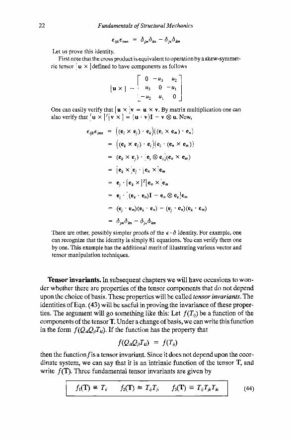
22 Fundamentals of Structural Mechanics
Let us prove this identity. First note that the cross product is equivalent to operation by a skew-symmet
ric tensor [ u x ] defined to have components as follows
[ux ]
0 — W3 W2
W3 0 - W i
-U2 u^ 0
One can easily verify that [u x ]v = u x v. By matrix multiplication one can also verify that [u x ]^[v x ] = (u • v)I - v ® u. Now,
^ijk^imn = ((Ci X e ) • e )((e,- x em) ' e„)
= ((e, X e -) • e,)(e, • (e, x e;„))
= (e, xe^.)-[e/®e,](e, X e )
= [e, x ] e - [ e , x]e ,
= e - [ e , x]^[e„x]e,
= e- • [(e^- e„)I - e„ ® e Je ;,
= ^jm^kn - ^jn^km
There are other, possibly simpler proofs of the e-(3 identity. For example, one can recognize that the identity is simply 81 equations. You can verify them one by one. This example has the additional merit of illustrating various vector and tensor manipulation techniques.
Tensor invariants. In subsequent chapters we will have occasions to wonder whether there are properties of the tensor components that do not depend upon the choice of basis. These properties will be called tensor invariants. The identities of Eqn. (43) will be useful in proving the invariance of these properties. The argument will go something like this: Let f(Tij) be a function of the components of the tensor T. Under a change of basis, we can write this function in the form /(QikQjiTki). If the function has the property that
fiQu^QjiTki) = m;)
then the function/is a tensor invariant. Since it does not depend upon the coordinate system, we can say that it is an intrinsic function of the tensor T, and write /(T). Three fundamental tensor invariants are given by
A(T) = T, /^(T) = T^^, f,(T) = TJjJ^ (44)
Chapter 1 Vectors and Tensors 23
The proof that /i(T) is invariant is straightforward
/i(T) = ^« = QikQiiTki = dkiTki = Tkk
by the formula for change of basis, contracted to give T,,, and Eqn. (43). The invariance of the other two functions can be proved in a similar manner (see Problem 18). Any function of tensor invariants is itself a tensor invariant. We shall sometimes refer to the invariant functions /i(T), fiCT), and /3(T) as the primary invariants to distinguish them from other invariant functional forms.
The trace of a tensor is simply the sum of its diagonal components. We use the operator "tr" to designate the trace. Thus, tr(T) = T^ is the first invariant of the tensor T. The second and third invariants can also be expressed in terms of the trace operator. Let us introduce the notation of a tensor raised to a power asT^ = XT and T^ = TTT, where the components are given by the formula for products of tensors, Eqn. (36), as
[T ] . = T,„T„^ [r].. = T^T^T„j (45)
It should be evident that a tensor can be raised to any (integer) power. Taking the trace of T^ and T' gives ti{T^) = [T].. and tr(T^) = [X']... Using these expressions in Eqn. (45) we find that the three invariants can be equivalently cast in terms of traces of powers of the tensor X as
/,(T) = tr(T), /,(T) = tr(T^), f,(T) = tT{T) (46)
By extension, one can establish that f„(T) = tr (X") is an invariant of the tensor X for any value of n (see Problem 18). One can prove that the invariants for « > 4 can all be computed from the first three invariants (see Problem 19).
Eigenvalues and eigenvectors of symmetric tensors. A tensor has properties independent of any basis used to characterize its components. As we have just seen, the components themselves have mysterious properties called invariants that are independent of the basis that defines them. It seems reasonable to expect that we might be able to find a representation of a tensor that is canonical. Indeed, this canonical form is the spectral representation of the tensor that can be built from its eigenvalues and eigenvectors. In this section we shall build the mathematics behind the spectral representation of tensors.
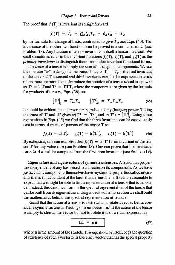
Recall that the action of a tensor is to stretch and rotate a vector. Let us consider a symmetric tensor X acting on a unit vector n.* If the action of the tensor is simply to stretch the vector but not to rotate it then we can express it as
Xn = jun (47)
where// is the amount of the stretch. This equation, by itself, begs the question of existence of such a vector n. Is there any vector that has the special property
24 Fundamentals of Structural Mechanics
that action by T is identical to multiplication by a scalar? Is it possible that more than one vector has this property?
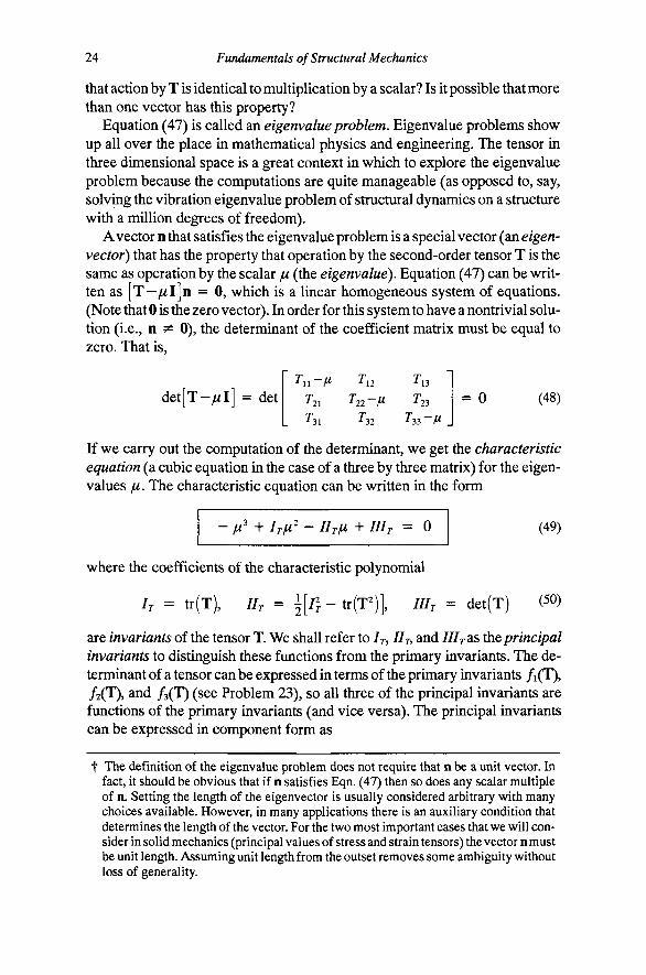
Equation (47) is called an eigenvalue problem. Eigenvalue problems show up all over the place in mathematical physics and engineering. The tensor in three dimensional space is a great context in which to explore the eigenvalue problem because the computations are quite manageable (as opposed to, say, solving the vibration eigenvalue problem of structural dynamics on a structure with a million degrees of freedom).
A vector n that satisfies the eigenvalue problem is a special vector (an eigenvector) that has the property that operation by the second-order tensor T is the same as operation by the scalar /u (the eigenvalue). Equation (47) can be written as [T—//l]n = 0, which is a linear homogeneous system of equations. (Note that 0 is the zero vector). In order for this system to have a nontrivial solution (i.e., n ^ 0), the determinant of the coefficient matrix must be equal to zero. That is.
det[T-//l] = det ^11 /^ ^12 ^13
^21 ^22 ~ /^ ^23
^31 ^32 ^33 ~f^
= 0 (48)
If we carry out the computation of the determinant, we get the characteristic equation (a cubic equation in the case of a three by three matrix) for the eigenvalues ju. The characteristic equation can be written in the form
- / / ' + IT/U^ - IITIU + IIIT = 0 (49)
where the coefficients of the characteristic polynomial
IT = tr(T), Ilr = \[n-tT(T% / / / , = det(T) (50)
are invariants of the tensor T. We shall refer to 7 , II T, and IIIT as the principal invariants to distinguish these functions from the primary invariants. The determinant of a tensor can be expressed in terms of the primary invariants /i(T), /2(T), and /^(T) (see Problem 23), so all three of the principal invariants are functions of the primary invariants (and vice versa). The principal invariants can be expressed in component form as
t The definition of the eigenvalue problem does not require that n be a unit vector. In fact, it should be obvious that if n satisfies Eqn. (47) then so does any scalar multiple of n. Setting the length of the eigenvector is usually considered arbitrary with many choices available. However, in many applications there is an auxiliary condition that determines the length of the vector. For the two most important cases that we will consider in solid mechanics (principal values of stress and strain tensors) the vector nmust be unit length. Assuming unit length from the outset removes some ambiguity without loss of generality.
Chapter 1 Vectors and Tensors 25
IT ~ Tih IIT = ^\I'iiI'i}''I'i}I'ij)^ IHT ~ "^^ijk^ImnTilTjmTkn (51)
Because the coefficients of the characteristic equation are invariants of the tensor T it follows that the roots// do not depend upon the basis chosen to describe the components and hence are intrinsic properties of T.
Finding the roots of the characteristic equation. The cubic equation has three roots (not necessarily distinct) that correspond to three (not necessarily unique) directions. If the cubic equation cannot be factored, then the roots can be found iteratively. For example, we can use Newton's method to solve the nonlinear equation g{x) = 0. Given a starting value x , we can compute successive estimates of a root of g(x) = 0 (see Chapter 12) as
Xi., X, ^,^^^ (52)
where g\x^ is the derivative of g{x) evaluated at the current iterate x,. The starting value determines the root to which the iteration converges if there are multiple roots. In the present context, let jc, be the estimate of the eigenvalue fi, at the /th iteration. The next estimate can be computed from Newton's formula as
_ 7x] - Ijx] + IIIT
""''' •" ?>x] - Tljx, + / / , ^ ^
The iteration continues until \xn — Xn-i\ is less than some acceptable tolerance. Then the eigenvalue is // « Xn^
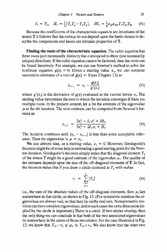
We can always take, as a starting value, Xo = 0. However, Gershgorin's theorem might be of some help in estimating a good starting point for the Newton iteration. Gershgorin's theorem simply states that the diagonal element Ta of the tensor T might be a good estimate of the eigenvalue fit. The quality of the estimate depends upon the size of the off-diagonal elements of T. In fact, the theorem states that if you draw a circle centered at Tu with radius
ri
•3
= Y.\^i^ (54)
i.e., the sum of the absolute values of the off-diagonal elements, then ///lies somewhere in that circle, as shown in Fig. 13. (For symmetric matrices the eigenvalues are always real, so that they lie on the real axis. Nonsymmetric matrices can have complex eigenvalues, and in such cases the extra dimension implied by the circle is important.) There is a catch. If two circles overlap, then the only thing we can conclude is that both of the two associated eigenvalues lie somewhere in the union of those two circles. For the case illustrated in Fig. 13, we know that Tss — ra < / a < T^^ + r^. We also know that the other two
26 Fundamentals of Structural Mechanics
Figure 13 Graphical representation of Gershgorin's theorem
eigenvalues satisfy T^-r^ < //ij/^i ^ 722 + 2, i.e., they lie somewhere between extremes of the two circles. Qearly, if the off-diagonal elements of the tensor are small, the diagonal elements are very good estimates of the eigenvalues. In any case, the diagonal elements should be good starting points for the Newton iteration. It also provides a means of checking our eigenvalues once we have found them. If they do not lie within the proper bounds, they cannot be correct. This theorem applies to matrices of any dunension.
Once one root is determined, one can use synthetic division to factor the root out of the cubic, leaving a quadratic that can be solved by the quadratic formula. Alternatively, we could simply use Eqn. (53) from another starting point in the hope that it would converge to one of the other roots (there is no guarantee that the iteration will converge to a root different from one already found).
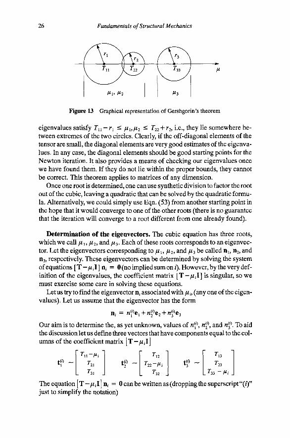
Determination of the eigenvectors. The cubic equation has three roots, which we call //1, // 2 > and /u 3. Each of these roots corresponds to an eigenvector. Let the eigenvectors corresponding to //i, //2? and fi^ be called ni, n2, and ns, respectively. These eigenvectors can be determined by solving the system ofequations[T-//J] n, = 0 (no implied sum on/). However, by the very definition of the eigenvalues, the coefficient matrix [T—//,I] is singular, so we must exercise some care in solving these equations.
Let us try to find the eigenvector n, associated with fi „ (any one of the eigenvalues). Let us assume that the eigenvector has the form
n,- = nfe,-^nfe2-\'nfe^
Our aim is to determine the, as yet unknown, values of nf, nf, and nf. To aid the discussion let us define three vectors that have components equal to the columns of the coefficient matrix [ T —/i,l]
t^P -Tn-f^i
T21
. T31
tf~ Tn
Tii-Hi
. 7'32 .
if ~ T» Tt^
.Ti3-fl
The equation [ T - / / , I ] n, = 0 can be written as (droppmg the superscript"(/)" just to simplify the notation)
Chapter 1 Vectors and Tensors 27
niti + Uiij + Wsta = 0 (55)
It should first be obvious that the vectors {ti, t2, U} are not linearly independent. In fact, we selected //1 precisely to create this linear dependence. Besides, if these vectors were linearly independent then, by a theorem of linear algebra, the only possible solution to Eqn. (55) would be «! =^2 = ^3 = 0, which is clearly at odds with our original aim.
Consider the case where the eigenvalue //, is distinct (i.e., neither of the other two eigenvalues is equal to it). In this case at least two of the three vectors {ti, t2, ta} are linearly independent. The trouble is we do not know in advance which two. There are three possibilities: {ti, ii), {ti, ts}, and {ts, U}. We can write Eqn. (55) as
^a^a'^^^^^ ~~ ^y^y (56)
ta
h •ta
ta
ta
t/> •*M ^A
ria
L« . = — «„ *y
ta
. * / >
•ty
ty
where no summation is implied and the integers {a, , y } take on distinct values of 1,2, or 3 (i.e., no two can be the same). Our three choices are then {a, )8, y} = {1,2,3}, {2,3,1}, or {3,1,2}. Equation (56) is overdetermined. There are more equations (3) than unknowns (2). However, by construction these equations should be consistent with each other. Hence, any two of the equations should be sufficient to determine ria and n^. To remove the ambiguity we can replace Eqn. (56) with its normal form by taking the dot product first with respect to ta and then with respect to t to give two equations in two unknowns:
(57)
Among the three choices of {a, j8, y} at least one must work. Equation (57) will not be solvable if the coefficient matrix is singular. That would be true if its determinant was zero, i.e., if (t^ ' ta)[t^ ' t^) = [ta ' t^)^. If this is the case then it is also true that riy = 0, which can certainly be verified once you have successfully solved the problem. If your first choice of {a, , y} did not work out, then try another one.
One of the important things to notice from Eqn. (57) is that ria and n^ can only be determined up to an arbitrary multiplier riy. To solve the equations one can simply specify a value of riy (riy = 1 will work just fine). The vector can be scaled by a constant g to give the final vector n = (waCa + Az e H-WyCyj. The condition of unit length of n establishes the value of g as
g = {nl^nl^nl) -1/2 (58)
Orthogonality of the eigenvectors. One interesting feature of the eigenvalue problem is that the eigenvectors for distinct eigenvalues are orthogonal, as suggested in the following lemma.
28 Fundamentals of Structural Mechanics
Lemma. Let n, and n be eigenvectors of the symmetric tensor T corresponding to distinct eigenvalues /// and /Uj, respectively (that is, they satisfy Tn = /un). Then n, is orthogonal to n , i.e., iij • n = 0.
Proof. The proof is based on taking the difference of the products of the eigenvectors with T in different orders (no summation on repeated indices)
0 = n - Tn, - n, • Tn
= n - • (//,n,) - n,- • {/Ujiij) (59)
The first line of the proof is true by definition of symmetry of T. The second line substitutes the eigenvalue property Tn = //n. The last line reflects that the dot product of vectors is commutative. Since we assumed that the eigenvalues were distinct, Eqn. (59)c can be true only if n, • Tij = 0, that is, if they are orthogonal. Q
Notice that orthogonality does not hold if the eigenvalues are repeated because Eqn. (59)c is satisfied even if n, • n r^ 0. We will see the ramification of this observation in the following examination of the special cases.
Special cases. There are two special cases that deserve mention. Both correspond to repeated roots of the characteristic equation. The main concern is how to find the eigenvectors associated with repeated roots.
If jUa = ju^ ^ fly we have the case that two of the roots are equal, but the third is distinct. For the distinct root fiy we can follow the above procedure and find the unique eigenvector n . The vectors corresponding to the double eigenvalue are not unique. If we have two eigenvectors n^ and n^ corresponding to ILta = lLCp = /i, then any vector that is a linear combination of those two vectors, n = ana + bn^, is also an eigenvector. The proof is simple
Tn = T[ana + bn^)
= oTna^bTn^
= afiUa-^-b/unp
= iu[ana-^bn^) = /un
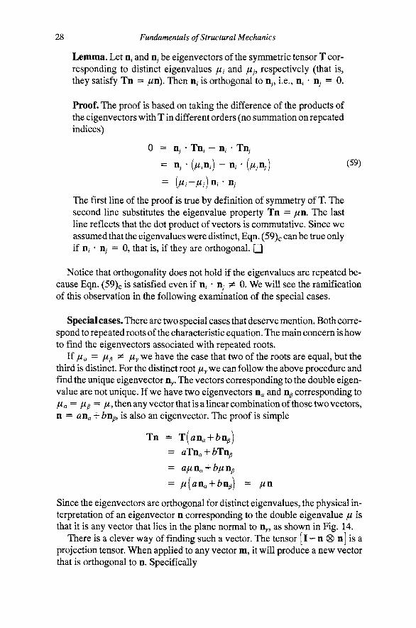
Since the eigenvectors are orthogonal for distinct eigenvalues, the physical interpretation of an eigenvector n corresponding to the double eigenvalue // is that it is any vector that lies in the plane normal to n , as shown in Fig. 14.
There is a clever way of finding such a vector. The tensor [l — n 0 n] is a projection tensor. When applied to any vector m, it will produce a new vector that is orthogonal to n. Specifically
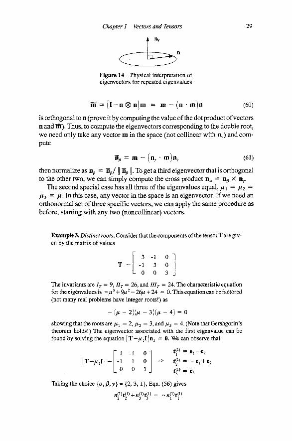
Chapter 1 Vectors and Tensors 29
Figure 14 Physical interpretation of eigenvectors for repeated eigenvalues
m = [ l - n 0 n]m = m - (n • m)n (60)
is orthogonal to n (prove it by computing the value of the dot product of vectors n and m). Thus, to compute the eigenvectors corresponding to the double root, we need only take any vector m in the space (not collinear with n ) and compute
= m — (iiy • mjiiy (61)
then normalize as n^ = n^/ || n ||. To get a third eigenvector that is orthogonal to the other two, we can simply compute the cross product n^ = n^ X n .
The second special case has all three ofthe eigenvalues equal,/^i = //2 = fii = //.In this case, any vector in the space is an eigenvector. If we need an orthonormal set of three specific vectors, we can apply the same procedure as before, starting with any two (noncollinear) vectors.
Example 3. Distinct roots. Consider that the components of the tensor T are given by the matrix of values
T -3 - 1 0
- 1 3 0 L 0 0 3
The invariants are Ij = 9, IIj = 26, and IIIj = 24. The characteristic equation for the eigenvalues is -/ i^ + 9/i^-26//-l-24 = 0. This equation can be factored (not many real problems have integer roots!) as
- ( / / - 2 ) ( / ^ - 3 ) ( / / - 4 ) = 0
showing that the roots are //j = 2, //2 = 3, and //3 = 4. (Note that Gershgorin's theorem holds!) The eigenvector associated with the first eigenvalue can be found by solving the equation [T-//il]ni = 0. We can observe that
[ T - ^ i l ] -
Taking the choice {a, )3, y} = {2, 3,1}, Eqn. (56) gives
1 -1 0
-1 1 0
0" 0 1 _
=> tf) = e,-e, t « = -ei+e^
t(') = 63
30 Fundamentals of Structural Mechanics
Letting n^^^ = 1, the normal equations, Eqn. (57), take the form
2 0 0 1
which gives n^^^ = 1 and n^^^ = 0. Thus, the eigenvector for / ^ = 2 is
Hj = Ci + 62
The remaining two eigenvectors can be found in exactly the same way, and are
02 = 63, n3 = Ci - 62
These vectors can, of course, be normalized to unit length.
It is interesting to note what happens for other choices of the normal equations in the preceding example. In particular, it is evident that t ^ = - tf\ If we were to make the choice {a,)S,y} = {l,2,3} then the coefficient matrix for the normal equations would be singular. This observation is also consistent with the fact that n ^ = 0.
Example 4. Repeated roots. Consider that the components of the tensor T are given by the matrix of values
5 1 1
-1 5
-1
-1 -1 5
The invariants are Ij = 15, IIj = 72, and IIIj = 108. The characteristic equation for the eigenvalues is
- ju^ + 15//2 - 72^ + 108 = 0
or - ( ^ - 3 ) ( ^ - 6 ) ( / . - 6 ) = 0
showing that the roots are/^i = ^2~ 6, and//3 = 3. The eigenvector associated with the distinct eigenvalue fi^ can be found by solving the equation [T—//3l]n3 = 0 as in the previous example. The result is
"3 = ^ ( € 1 + 6 2 + 63)
The eigenvectors corresponding to the repeated root must lie in a plane orthogonal to 03. We can select any vector in the space and project out the component along 03. Let us use m = e . Project out the part of the vector along 03 (see Example 1)
Chapter 1 Vectors and Tensors 31
n2 = ^Pm = ^[l-n3 (g) njjej
= ^[ei-(n3 -ejns]
= ^[^1 -^(€1+62 + 63)]
= ^(1^1-^62-563)
= ^(261-62-63)
where the constant Q was selected to give the vector unit length. Finally, iii can be computed as n = 02 x n3 to give
Hi = ^ ( - e 2 + e. fi 31
The spectral decomposition. If the eigenvalues and eigenvectors are known, we can express the original tensor in terms of those objects in the following manner
3
T = 2]/^,n,(g)n, / = 1
(62)
Note that we need to suspend the summation convention because of the number of times that the index / appears in the expression. This form of expression of the tensor T is called the spectral decomposition of the tensor. How do we know that the tensor T is equivalent to its spectral decomposition? As we indicated earlier, the operation of a second-order tensor is completely defined by its operation on three independent vectors. Let us assume that the eigenvectors {Oi, n2, 03} are orthogonal (which means that any eigenvectors associated with repeated eigenvalues were orthogonalized). Let us examine how the tensor and its spectral decomposition operate on n
3 3 3
Tnj = ^ / / / [ n , ® nj n,- = ^/^/(ny • n,) n,- = ^//,(3yn, = /Ujiij i = l i = l / = 1
Thus, we have concluded that both tensors operate the same way on the three eigenvectors. Therefore, the spectral representation must be equivalent to the original tensor. A corollary of the preceding construction is that any two tensors with exactly the same eigenvalues and eigenvectors are equivalent.
The spectral decomposition affords us another remarkable observation. We know that we are free to select any basis vectors to describe the components of a tensor. What happens if we select the eigenvectors {DI, 02, n3} as the basis? According to Eqn. (62), in this basis the off-diagonal components of the tensor T are all zero, while the diagonal elements are exactly the eigenvalues
32 Fundamentals of Structural Mechanics
i " l
0 0
0 fl2
0
0 0 f^3
T -
The invariants of T also take a special form when expressed in terms of the eigenvalues. The invariants are, by their very nature, independent of the basis chosen to represent the tensor. As such, one must get the same value of the invariants in all bases. Those values will, of course, be the values computed in any specific basis. The simplest basis, often referred to as the canonical basis, is the one given by the eigenvectors. In this basis, the invariants can be represented as
IT = fl^+lU2-^iU3
IIT = / / I / / 2 + / ^ I / ^ 3 + / ^ 2 / ^ 3
IIIT = fli/U2/il3
(63)
Example 5. Consider a tensor T that has one distinct eigenvalue ju^ and a repeated eigenvalue / 2 = /^s- Use the spectral decomposition to show that the tensor T can be represented as
T = /^i[n(8)n] + iLL2[l-n®n]
where n is the unit eigenvector associated with the distinct eigenvalue ju^. Let Dj = n, n2, and n^ be eigenvectors of T. Further assume that these vec
tors are orthogonal (remember, if they are not orthogonal due to a repeated root, they can always be orthogonalized). The sum of outer products of orthonormal vectors is the identity. Thus,
3 3
I = V n ® n, = n 0 n -H V n, 0 n, i = l i=2
Write T in terms of its spectral decomposition as
3 3
T = ^/^ , [n ,®n,] = /^in®n + 2 / i J n , ® n , ] 1=1 1=2
3
= fi^n (Sin-\-ju 2^ ni(Sini 1 = 2
= fi^n ® n + jU2[l - n ® n]
There is great significance to this result. Notice that the final spectral representation does not refer to n2 and 03 at all. Since these vectors are arbitrarily chosen from the plane orthogonal to n these vectors have no intrinsic significance (other than that they faithfully represent the plane). In this case there are only three in-

Chapter 1 Vectors and Tensors 33
trinsic bits of information: /z , 1^2^ and n. Hence, this representation of T is canonical.
The Cayley-Hamilton theorem. The spectral decomposition and the characteristic equation for the eigenvalues of a tensor can be used to prove the Cayley-Hamilton theorem, which states that
T - IjT^ + IIjT - IIIjl = 0 (64)
where T^ = TTandT^ = TTT are products of the tensor T with itself. Using the spectral decomposition, one can show that (Problem 22)
3
1 = 1
Using this result, and noting that I = n, (S) n, (sum implied), we can compute
3
T ~ IjT + II/T - IIIjl = Yj^fi] - Ijfi] + Ilrti, - IIIr)n, ® n, t = i
All of the eigenvalues satisfy the characteristic equation. Thus, the term in parentheses is always zero, thereby proving the theorem.
Vector and Tensor Calculus Afield is a function of position defined on a particular region. In our study of mechanics we shall have need of scalar, vector, and tensor fields, in which the output of the function is a scalar, vector, or tensor, respectively. For problems defined on a region of three-dimensional space, the input is the position vector X. A function defined on a three-dimensional domain, then, is a function of three independent variables (the components jCi, X2y and X3 of the position vector x). In certain specialized theories (e.g., beam theory, plate theory, and plane stress) position will be described by one or two independent variables.
A field theory is a physical theory built within the framework of fields. The primary advantage of using field theories to describe physical phenomena is that the tools of differential and integral calculus are available to carry out the analysis. For example, we can appeal to concepts like infinitesimal neighborhoods and limits. And we can compute rates of change by differentiation and accumulations and averages by integration.
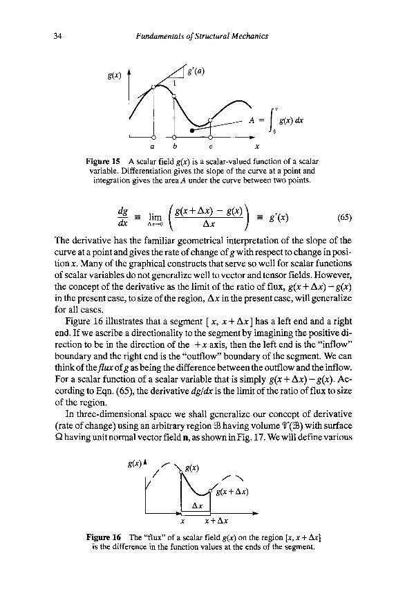
Figure 15 shows the simplest possible manifestation of a field: a scalar function of a scalar variable, g(x), A scalar field can, of course, be represented as a graph with x as the abscissa and g{x) as the ordinate. For each value of position X the function produces as output g(x). The derivative of the function is defined through the limiting process as
34 Fundamentals of Structural Mechanics
gW
Figure 15 A scalar field g{x) is a scalar-valued function of a scalar variable. Differentiation gives the slope of the curve at a point and integration gives the area A under the curve between two points.
-— = lim ax AJC-O
g(x + Ax) - g{x) Ax ^ g\^) (65)
The derivative has the familiar geometrical interpretation of the slope of the curve at a point and gives the rate of change of g with respect to change in position X. Many of the graphical constructs that serve so well for scalar functions of scalar variables do not generalize well to vector and tensor fields. However, the concept of the derivative as the limit of the ratio of flux, g{x + AJC) — g{x) in the present case, to size of the region. Ax in the present case, will generalize for all cases.
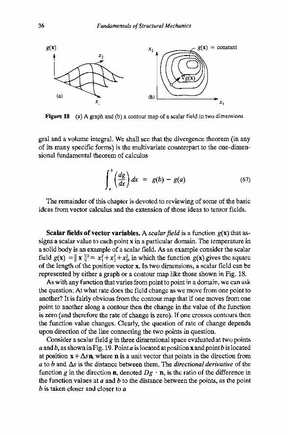
Figure 16 illustrates that a segment [ x, x + Ax] has a left end and a right end. If we ascribe a directionality to the segment by imagining the positive direction to be in the direction of the +x axis, then the left end is the "inflow" boundary and the right end is the "outflow" boundary of the segment. We can think of the/Zwx of g as being the difference between the outflow and the inflow. For a scalar function of a scalar variable that is simply g(x + Ax) - g(x). According to Eqn. (65), the derivative dgldx is the limit of the ratio of flux to size of the region.
In three-dimensional space we shall generalize our concept of derivative (rate of change) using an arbitrary region S having volume T(98) with surface Q having unit normal vector field n, as shown in Fig. 17. We will define various
W
Kl 1 ^
,?w
M Ax
^ X ^ ( x + Ax)
•
X x + Ax
Figure 16 The "flux" of a scalar field g(x) on the region [x, x + Ax] is the difference in the function values at the ends of the segment.

Chapter 1 Vectors and Tensors 35
Figure 17 A region 3& in three-dimensional space with volume T(^) and surface Q with outward unit normal vector field n.
types of derivatives of various types of fields in the following sections, but all of these derivatives will be the limit of the ratio of some sort of flux (outflow minus inflow) to the volume of the region as the volume shrinks to zero. In these definitions the flux will involve an integral over the surface area and the normal vector n will help to distinguish "inflow" from "outflow" for the situation at hand. For each definition of derivative we will develop a coordinate expression that will tell us how to formally "take the derivative" of the field. The coordinate expressions will all involve partial derivatives of the vector or tensor components.
The integral of the function between the limits b and c gives the area between the graph of the function g{x) and the x axis (see Fig. 15). For any scalar function of a scalar variable one can think of the integral as the "area under the curve." Integration is the limit of a sum of infinitesimal strips with area g{x)dx. The total area is the accumulated sum of the infinitesimal areas. The geometric notion of integration is quite independent of techniques of integration based upon anti-derivatives of functions because there are methods of integration (e.g., numerical quadrature) that do not rely upon the anti-derivative. In our developments here we need to think of integrals both in the sense of executing integrals (mostly later in the book) and in the more generic sense of accumulating the limit of a sum.
In three dimensional space we will encounter surface integrals and volume integrals. Most of the time we will not use the notation of "double integrals" for surface integrals and "triple integration" for volume integrals, but rather understand that
\[')dA= j \[')dxdy, \[')dy= j j \{')dxdydz (66)
where the variables and infinitesimals must be established for the coordinate system that is being used to characterize the problem at hand. Again, techniques of integration are important only in particular problems to carry out computations.
The second aspect of integration that we will introduce in this chapter is the idea of integral theorems that provide an equivalence between a surface inte-
36 Fundamentals of Structural Mechanics
g(x) x^ ^ ^(x) = constant A X,
(a)
Figure 18 (a) A graph and (b) a contour map of a scalar field in two dimensions
gral and a volume integral. We shall see that the divergence theorem (in any of its many specific forms) is the multivariate counterpart to the one-dimensional fundamental theorem of calculus
-f a
^)dx = g{b)-g{a) (67)
The remainder of this chapter is devoted to reviewing of some of the basic ideas from vector calculus and the extension of those ideas to tensor fields.
Scalar fields of vector variables. A scalar field is a function g(x) that assigns a scalar value to each point x in a particular domain. The temperature in a solid body is an example of a scalar field. As an example consider the scalar field g(x) = II X p = jCi + A:2+JC3, in which the function g(x) gives the square of the length of the position vector x. In two dimensions, a scalar field can be represented by either a graph or a contour map like those shown in Fig. 18.
As with any function that varies from point to point in a domain, we can ask the question: At what rate does the field change as we move from one point to another? It is fairly obvious from the contour map that if one moves from one point to another along a contour then the change in the value of the function is zero (and therefore the rate of change is zero). If one crosses contours then the function value changes. Qearly, the question of rate of change depends upon direction of the line connecting the two points in question.
Consider a scalar field g in three dimensional space evaluated at two points a and fc, as shown in Fig. 19. Point a is located at position x and point b is located at position x + Asn, where n is a unit vector that points in the direction from aXob and As is the distance between them. The directional derivative of the function g in the direction n, denoted Dg • n, is the ratio of the difference in the function values at a and b to the distance between the points, as the point b is taken closer and closer to a
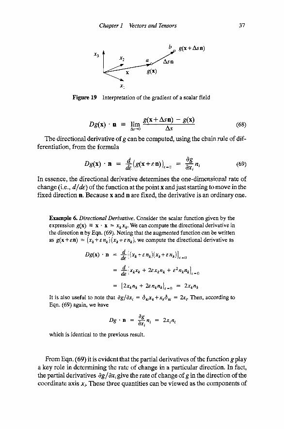
Chapter 1 Vectors and Tensors 37
Figure 19 Interpretation of the gradient of a scalar field
Dg{x) • n = lim g(x + Ayn) -g (x )
^s (68)
The directional derivative of g can be computed, using the chain rule of differentiation, from the formula
Dg(x)'n = - |(g(x + n ) t , = ^n, da (69)
In essence, the directional derivative determines the one-dimensional rate of change (i.e., d/de) of the function at the point x and just starting to move in the fixed direction n. Because x and n are fixed, the derivative is an ordinary one.
Example 6. Directional Derivative. Consider the scalar function given by the expression g(x) = x • x = oc jc . We can compute the directional derivative in the direction n by Eqn. (69). Noting that the augmented function can be written as g(x + en) = (xk + en^) (xi^-\'enk), we compute the directional derivative as
^^(x) • n = ^{(x,, + en,,)(xk + en,,)]^^^
= -^{^kXk + ^xi,n^ + e^nj,nk]^^Q
= {^x^n^ + lenknkl^Q = 2^ /i
It is also useful to note that dg/dx^ = dj^Xi^-^x^d,^ = 2;c,. Then, according to Eqn. (69) again, we have
which is identical to the previous result.
From Eqn. (69) it is evident that the partial derivatives of the function g play a key role in determining the rate of change in a particular direction. In fact, the partial derivatives dg/dxigiv^ the rate of change of g in the direction of the coordinate axis x,. These three quantities can be viewed as the components of
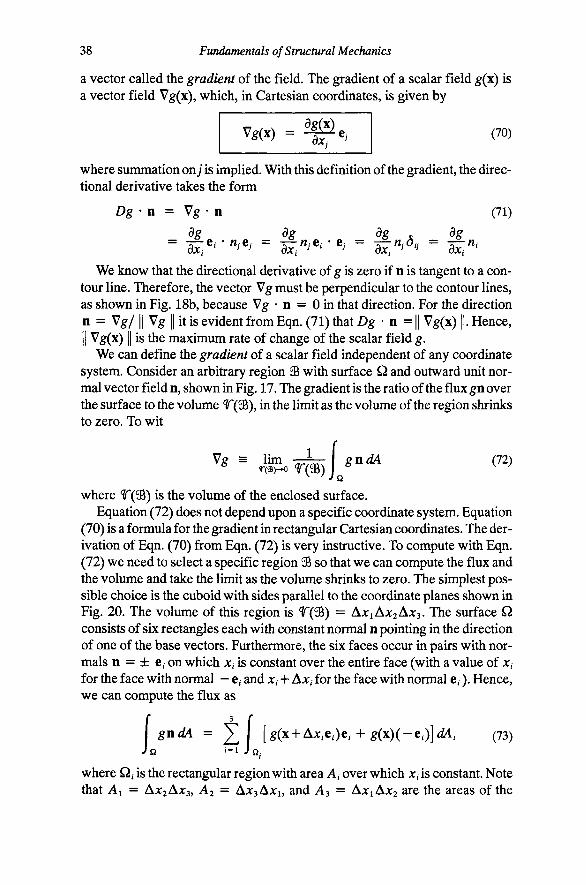
38 Fundamentals of Structural Mechanics
a vector called the gradient of the field. The gradient of a scalar field g(\) is a vector field Vg(x), which, m Cartesian coordinates, is given by
Vs(x) = ^ . , dXj (70)
where summation on; is implied. With this definition of the gradient, the directional derivative takes the form
Dg-n = Vgn (71)
^g ^g dg X ^g
We know that the directional derivative of g is zero if n is tangent to a contour line. Therefore, the vector Vg must be perpendicular to the contour lines, as shown in Fig. 18b, because Vg • n = 0 in that direction. For the direction ^ = ^g/ II ^g II it is evident from Eqn. (71) that Dg • n = || Vg(x) ||. Hence, II Vg(x) II is the maximum rate of change of the scalar field g.
We can define the gradient of a scalar field independent of any coordinate system. Consider an arbitrary region 99 with surface Q and outward unit normal vector field n, shown in Fig. 17. The gradient is the ratio of the flux gn over the surface to the volume T(98), in the limit as the volume of the region shrinks to zero. To wit
^g = lim : ; 7 ^ gndA (72) ^ r(a)-o r(as)J ^ ^ ^
where T(93) is the volume of the enclosed surface. Equation (72) does not depend upon a specific coordinate system. Equation
(70) is a formula for the gradient in rectangular Cartesian coordinates. The derivation of Eqn. (70) from Eqn. (72) is very instructive. To compute with Eqn. (72) we need to select a specific region 98 so that we can compute the flux and the volume and take the limit as the volume shrinks to zero. The simplest possible choice is the cuboid with sides parallel to the coordinate planes shown in Fig. 20. The volume of this region is T(95) = AjCi AA:2AJC3. The surface Q consists of six rectangles each with constant normal n pointing in the direction of one of the base vectors. Furthermore, the six faces occur in pairs with normals n = ± e, on which jc, is constant over the entire face (with a value of Xi for the face with normal - e, and jc, + Ax, for the face with normal e,). Hence, we can compute the flux as
gntM = ^ [g(x + Ax,e,)e, + g ( x ) ( - e , ) ] ^ , (73)
where Q, is the rectangular region with area A, over which jc, is constant. Note that Ai = AX2AX2, A2 = AJC3AJC1, and A3 = AjCiAxj are the areas of the
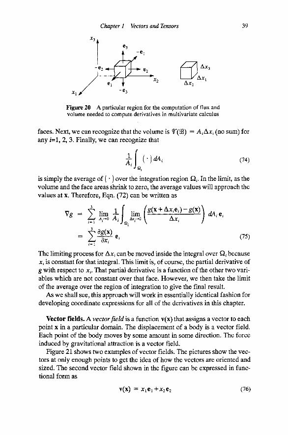
Chapter 1 Vectors and Tensors 39
/Z7\ AJCO
Ax I/AXI
Figure 20 A particular region for the computation of flux and volume needed to compute derivatives in multivariate calculus
faces. Next, we can recognize that the volume is T(9B) = AiAXi (no sum) for any /=1, 2, 3. Finally, we can recognize that
J Q
{')dA, (74)
is simply the average of (•) over the integration region Q,. In the limit, as the volume and the face areas shrink to zero, the average values will approach the values at x. Therefore, Eqn. (72) can be written as
V g = X ' t a i - f un, («( '+A»e,)-^x)\
= 1 MO dXi
e,- (75)
The limiting process for AJC can be moved inside the integral over Q, because Xi is constant for that integral. This limit is, of course, the partial derivative of g with respect to jc,. That partial derivative is a function of the other two variables which are not constant over that face. However, we then take the limit of the average over the region of integration to give the final result.
As we shall see, this approach will work in essentially identical fashion for developing coordinate expressions for all of the derivatives in this chapter.
Vector fields. A vector field is a function v(x) that assigns a vector to each point x in a particular domain. The displacement of a body is a vector field. Each point of the body moves by some amount in some direction. The force induced by gravitational attraction is a vector field.
Figure 21 shows two examples of vector fields. The pictures show the vectors at only enough points to get the idea of how the vectors are oriented and sized. The second vector field shown in the figure can be expressed in functional form as
v(x) = Xiei+jCjCs (76)
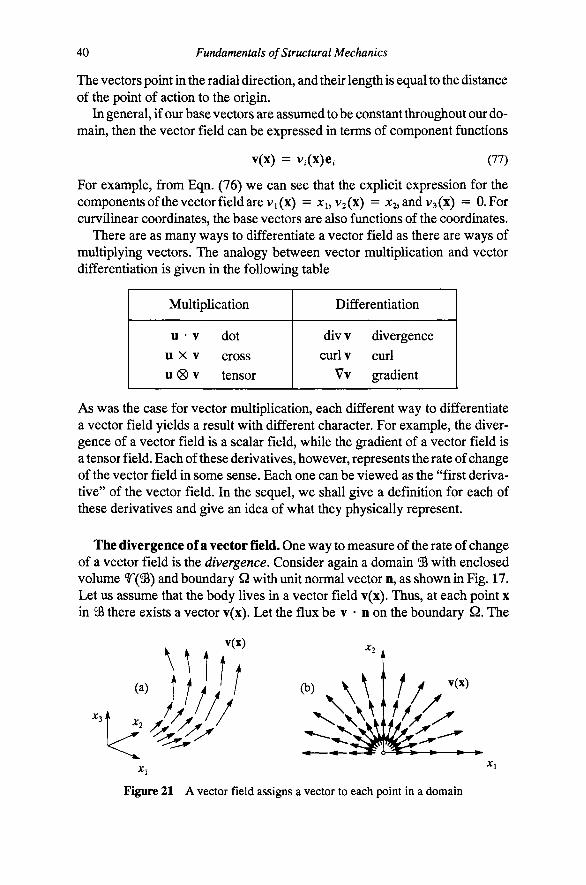
40 Fundamentals of Structural Mechanics
The vectors point in the radial direction, and their length is equal to the distance of the point of action to the origin.
In general, if our base vectors are assumed to be constant throughout our domain, then the vector field can be expressed in terms of component functions
v(x) = v,(x)e, (77)
For example, from Eqn. (76) we can see that the explicit expression for the components ofthe vector field are Vi(x) = jci, V2(x) = A:2,andv3(x) = O.For curvilinear coordinates, the base vectors are also functions ofthe coordinates.
There are as many ways to differentiate a vector field as there are ways of multiplying vectors. The analogy between vector multiplication and vector differentiation is given in the following table
Multiplication
u • V dot u X V cross u (g) V tensor
Differentiation
div V divergence curl V curl
Vv gradient
As was the case for vector multiplication, each different way to differentiate a vector field yields a result with different character. For example, the divergence of a vector field is a scalar field, while the gradient of a vector field is a tensor field. Each of these derivatives, however, represents the rate of change of the vector field in some sense. Each one can be viewed as the "first derivative" of the vector field. In the sequel, we shall give a definition for each of these derivatives and give an idea of what they physically represent.
The divergence of a vector field. One way to measure ofthe rate of change of a vector field is the divergence. Consider again a domain 95 with enclosed volume T(93) and boundary Q with unit normal vector n, as shown in Fig. 17. Let us assume that the body lives in a vector field v(x). Thus, at each point x in 95 there exists a vector v(x). Let the flux be v • n on the boundary Q, The
(b) v(x)
Figure 21 A vector field assigns a vector to each point in a domain
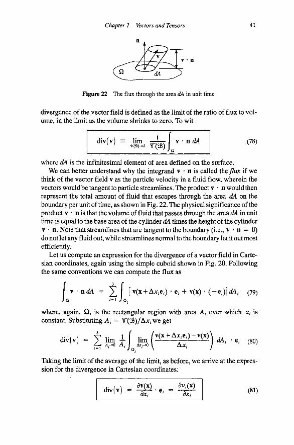
Chapter 1 Vectors and Tensors 41
V • n
Figure 22 The flux through the area dA in unit time
divergence of the vector field is defined as the limit of the ratio of flux to volume, in the limit as the volume shrinks to zero. To wit
div(v) = lim r(S)-K) n )J, y ' ndA (78)
where dA is the infinitesimal element of area defined on the surface. We can better understand why the integrand v • n is called the flux if we
think of the vector field v as the particle velocity in a fluid flow, wherein the vectors would be tangent to particle streamlines. The product v • n would then represent the total amount of fluid that escapes through the area dA on the boundary per unit of time, as shown in Fig. 22. The physical significance of the product V • n is that the volume of fluid that passes through the area dA in unit time is equal to the base area of the cylinder dA times the height of the cylinder V • n. Note that streamlines that are tangent to the boundary (i.e., v • n = 0) do not let any fluid out, while streamlines normal to the boundary let it out most efficiently.
Let us compute an expression for the divergence of a vector field in Cartesian coordinates, again using the simple cuboid shown in Fig. 20. Following the same conventions we can compute the flux as
V • n ^ = ^ [v(x + AA:,e,) • e, + v(x) • ( - e , ) ] ^ , (79)
where, again, Q, is the rectangular region with area A, over which jc, is constant. Substituting A, = T(95)/Ax, we get
''Mv) = g.onj:J.K.('<--^ff-"")^.-.. (30,
Taking the limit of the average of the limit, as before, we arrive at the expression for the divergence in Cartesian coordinates:
diviv = - av(x) ^ dv,(x)
dXi e/ = dXi (81)
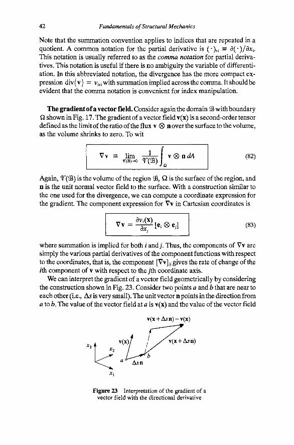
42 Fundamentals of Structural Mechanics
Note that the summation convention applies to indices that are repeated in a quotient. A common notation for the partial derivative is (• )„ = d( • )/dXi. This notation is usually referred to as the comma notation for partial derivatives. This notation is useful if there is no ambiguity the variable of differentiation. In this abbreviated notation, the divergence has the more compact expression div (V) = v„, with summation implied across the comma. It should be evident that the comma notation is convenient for index manipulation.
The gradient of a vector field. Consider again the domain 95 with boundary Q shown in Fig. 17. The gradient of a vector field v(x) is a second-order tensor defined as the limit of the ratio of the flux v (g) n over the surface to the volume, as the volume shrinks to zero. To wit
Vv = lim ^ ^ \®ndA (82)
Again, T(95) is the volume of the region % Q is the surface of the region, and n is the unit normal vector field to the surface. With a construction similar to the one used for the divergence, we can compute a coordinate expression for the gradient. The component expression for Vv in Cartesian coordinates is
v. = ^ [ . ® . , l (83)
where summation is implied for both / and;. Thus, the components of Vv are simply the various partial derivatives of the component functions with respect to the coordinates, that is, the component [Vv]y gives the rate of change of the ith component of v with respect to the ;th coordinate axis.
We can interpret the gradient of a vector field geometrically by considering the construction shown in Fig. 23. Consider two points a and b that are near to each other (i.e., A^ is very small). The unit vector n points m the direction from a to b. The value of the vector field at a is v(x) and the value of the vector field
v(x-f A5n)-
v(x- -Asn)
Figure 23 Interpretation of the gradient of a vector field with the directional derivative
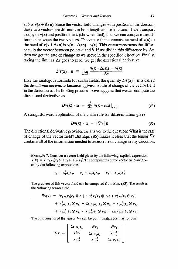
Chapter 1 Vectors and Tensors 43
at b is v(x + Asn). Since the vector field changes with position in the domain, these two vectors are different in both length and orientation. If we transport a copy of v(x) and position it at b (shown dotted), then we can compare the difference between the two vectors. The vector that connects the head of v(x) to the head of v(x H- A^n) is v(x + Asn) - v(x). This vector represents the difference in the vector between points a and fe. If we divide this difference by As, then we get the rate of change as we move in the specified direction. Finally, taking the limit as As goes to zero, we get the directional derivative
r. . . ,. v(x + A5n) - v(x) Dv(x) • n = lun - ^ ^ ^^
^ ^ As-K) As
Like the analogous formula for scalar fields, the quantity Z)v(x) • n is called the directional derivative because it gives the rate of change of the vector field in the direction n. The limiting process above suggests that we can compute the directional derivative as
Z)v(x)-n = ^ [ v ( x + £n)]^^^ (84)
A straightforward application of the chain rule for differentiation gives
Dv(x) • n = [Vv]n (85)
The directional derivative provides the answer to the question: What is the rate of change of the vector field? But Eqn. (85) makes it clear that the tensor Vv contains all of the information needed to assess rate of change in any direction.
Example 7. Consider a vector field given by the following explicit expression v(x) = JCj JC2;C3 (jCj Cj + ;c2 62 + x^ 63). The components of the vector field are given by the following expressions
Vj = X\X2X'^, V2 = X^xjXj, V3 = X1X2X1
The gradient of this vector field can be computed from Eqn. (83). The result is the following tensor field
Vv(x) = 2x^X2X^[ei ® e j + x^x^le^ (g) 63] + ^i^al^i ® ^3]
+ xlx^[e2 ® Cj] + 2XiJC2JC3[e2 ® 62] + XiX\[t2 ® 63]
+ ^ 2- 31 3 ® ^i] + ^l^3[e3 ® €2] + 2XiX2X2[t^ ® €3]
The components of the tensor Vv can be put in matrix form as follows
X\X2 2X10^2^3
•^2-^3
X2XI
A^3
2riJC2^3
Xixl 2x1^2X3
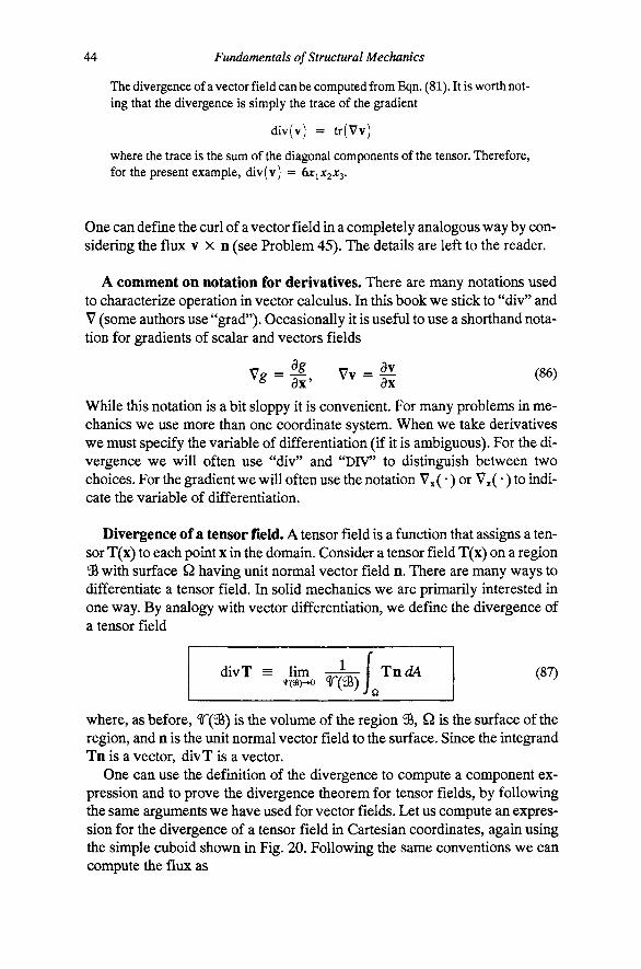
44 Fundamentals of Structural Mechanics
The divergence of a vector field can be computed from Eqn. (81). It is worth noting that the divergence is simply the trace of the gradient
div(v) = tr(Vy)
where the trace is the sum of the diagonal components of the tensor. Therefore, for the present example, div(v) = 6x1X20 3.
One can define the curl of a vector field in a completely analogous way by considering the flux VXD (see Problem 45). The details are left to the reader.
A comment on notation for derivatives. There are many notations used to characterize operation in vector calculus. In this book we stick to "div" and V (some authors use "grad"). Occasionally it is useful to use a shorthand notation for gradients of scalar and vectors fields
V;. = - ^ Vv = - ^ (86)
While this notation is a bit sloppy it is convenient. For many problems in mechanics we use more than one coordinate system. When we take derivatives we must specify the variable of differentiation (if it is ambiguous). For the divergence we will often use "div" and "DIV" to distinguish between two choices. For the gradient we will often use the notation ^x{')orV^(')to indicate the variable of differentiation.
Divergence of a tensor field. A tensor field is a function that assigns a tensor T(x) to each point x in the domain. Consider a tensor field T(x) on a region 3B with surface Q having unit normal vector field n. There are many ways to differentiate a tensor field. In solid mechanics we are primarily interested in one way. By analogy with vector differentiation, we define the divergence of a tensor field
divT ^ lim ^ ^ T n ^ U], (87)
where, as before, T(95) is the volume of the region % Q is the surface of the region, and n is the unit normal vector field to the surface. Since the integrand Tn is a vector, divT is a vector.
One can use the definition of the divergence to compute a component expression and to prove the divergence theorem for tensor fields, by following the same arguments we have used for vector fields. Let us compute an expression for the divergence of a tensor field in Cartesian coordinates, again using the simple cuboid shown in Fig. 20. Following the same conventions we can compute the flux as
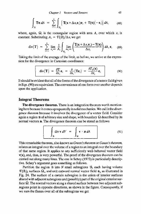
Chapter 1 Vectors and Tensors
I T n ^ = 5^1 [T(x + Ax,e,)e, + T(x)(-e,)]ti4,
45
(88)
where, again, Q, is the rectangular region with area A, over which x, is constant. Substituting A, = T(9&)/AJC/we get
Taking the limit of the average of the limit, as before, we arrive at the expression for the divergence in Cartesian coordinates:
*^Cf) = g " - ^C^") = e,- (90)
It should be evident that all of the forms of the divergence of a tensor field given in Eqn. (90) are equivalent. The convenience of one form over another depends upon the application.
Integral Theorems The divergence theorem. There is an mtegration theorem worth mention
ing here because it comes up repeatedly in solid mechanics. We call it the divergence theorem because it involves the divergence of a vector field. Consider again a region S of arbitrary size and shape, with boundary Q described by its normal vectors n. The divergence theorem can be stated as follows
divydV = ndA (91)
This remarkable theorem, also known as Green's theorem or Gauss's theorem, relates an integral over the volume of a region to an integral over the boundary of that same region. It applies to any sufficiently well-behaved vector field v(x), and, thus, is very powerful. The proof of the divergence theorem can be carried out along many lines. The one in Schey (1973) is particularly descriptive. Schey's argument goes something as follows.
Partition the region 3B into N small subregions S, each having volume T(98/), surfaces Q„ and unit outward normal vector field n„ as illustrated in Fig. 24. The surface of a certain subregion is the union of interior surfaces shared with adjacent subregions and (possibly) part of the original exterior surface Q. The normal vectors along a shared surface between two adjacent sub-regions point in opposite directions, as shown in the figure. Consequently, if we sum the fluxes over all of the subregions we get
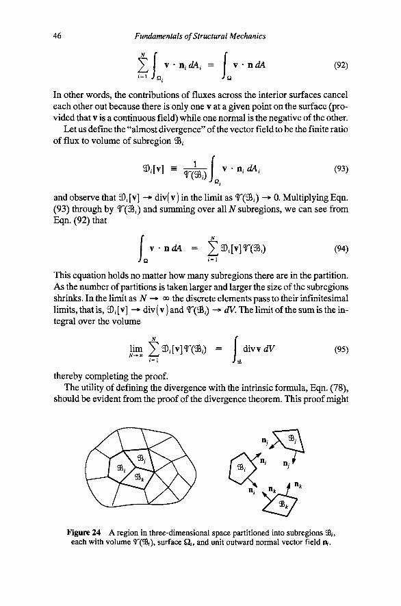
46 Fundamentals of Structural Mechanics
'=1 JQ: JQ
(92)
In other words, the contributions of fluxes across the interior surfaces cancel each other out because there is only one v at a given point on the surface (provided that V is a continuous field) while one normal is the negative of the other.
Let us define the "almost divergence" of the vector field to be the finite ratio of flux to volume of subregion 3S,
9)/[v] r(%)j^ n, dA, (93)
and observe that 3)/[v] -> div(v) in the limit as T(95/) -> 0. Multiplying Eqn. (93) through by T(95,) and summing over all N subregions, we can see from Eqn. (92) that
I V • n ^ = Ja ) , [v ] r (S , ) (94)
This equation holds no matter how many subregions there are in the partition. As the number of partitions is taken larger and larger the size of the subregions shrinks. In the limit as iV -^ oo the discrete elements pass to their infinitesimal limits, that is, 3) [v] ^ div (v) and r(3i,) -> dV, The limit of the sum is the integral over the volume
lim ^3) i [v ] r (a , ) = di diw dV (95)
thereby completing the proof. The utility of defining the divergence with the intrinsic formula, Eqn. (78),
should be evident from the proof of the divergence theorem. This proof might
Figure 24 A region in three-dimensional space partitioned into subregions %, each with volume T(%\ surface Qj, and unit outward normal vector field n,.

Chapter 1 Vectors and Tensors 47
not have the level of rigor that a mathematician would like (the limiting process and crossover to infinitesimals being the sloppiest point), but the geometric basis lends it a clarity that is more than adequate for our purposes here.
The divergence theorem holds for any vector field v(x) that is well behaved. A simple way to think about "well-behavedness" is to consider some of the bad things that might happen on the way to the limit. In particular, any of the objects, like 9),[v], must exist for all possible subdivisions. If the vector field has a singular point (v -^ oo), then eventually the subdivision process will encounter it, and, for the subdomains on whose boundaries the singularity lies, 3)/[v] is not defined. Similarly, if the field has a bounded jump along some surface (where v~ T^ V" on opposites sides of the jump), then for those subdomains that have a boundary on the jump surface, the fluxes will not cancel out. Many of these pathologies can be treated by enhancing the integral theorems with features that account for them. We do not have to worry about the pathologies if our vector field v and its divergence are continuous over the domain 98 and on the surface Q.
Example 8. The divergence theorem for the gradient of a scalar field is
\dA ^gdV = gm
where 9B is a region with surface Q having unit outward normal vector field n. Verify the relationship by applying it to the function g = x\+x\+x\ defined on a cylinder of unit radius and unit height, centered at the origin.
'"y\^ n = tr
Figure 25 Circular cylinder definition for Example 8.
The integral of the gradient over the volume is best done in cylindrical coordinates. Let Xj = r cos 0, Xj = r sin d, and x^ = z. The gradient of g can be computed as Vg = 2x = 2[rtr-^zt^), where tr{B) = cos^Cj-H sin^ej. The volume integral can be carried out as follows:
I VgdV = I f f 2(re,(^) JaJ Jo Jo Jo
^zt^)rdrdOdz = JtR^h^e^
(Observe that the integral of er(0) with respect to 6 from 0 to 27r is zero). The surface has the following characteristics:
48 Fundamentals of Structural Mechanics
Bottom Surface: z = 0 n = - e 3 g = r^
Top Surface: z = h n = +63 g = r^ + h^
Lateral Surface: r = R n = C;. g = R^^-z^
The surface integral can be carried out as follows, noting that the integrand for the top and bottom surfaces reduces to (r^ + /i^)e3 - r^e3 = h^t^,
gndA = h^t^rdrde+ {R^ + z^)er(e)RdO dz JQ JO JO JO JO
= TtR^h^e^
Qearly, the volume and surface integrals have the same value, as the divergence theorem promises.
There are integral theorems for the gradient of a scalar field, the gradient of a vector field and a tensor field (see next section) that are analogous to the divergence theorem. The statements and proofs of these theorem are left as an exercise (Problem 46).
Divergence theorem for tensor fields. Any tensor field satisfies the following integral theorem (divergence theorem)
divTJy = TndA Ja JQ
(96)
where, as before, T(93) is the volume of the region % Q is the surface of the region, and n is the unit normal vector field to the surface. Proof of the divergence theorem for tensor fields is left as an exercise (Problem 46).
Additional Reading
M. E. Gurtin, A« introduction to continuum mechanics, Academic Press, 1981.
H, M. Schey, Div, grad, curl, and all that, Norton, New York, 1973.
J. G. Simmonds, A brief on tensor analysis. Springer-Verlag, New York, 1982.
J. H. Wilkinson, The algebraic eigenvalue problem, Oxford University Press, Oxford, 1965.
Chapter 1 Vectors and Tensors 49
Problems 1. Compute the values of the following expressions
(a) d, (b) (5,(3,
(d) daijdf^dcd "• dxydyz (enough terms to exhaust the whole alphabet)
2. Let two vectors, u and v, have components relative to some basis as u = (5, - 2,1) and V = (1,1,1). Compute the lengths of the vectors and the angle between them. Find the area of the parallelogram defined by u and v.
3. The vertices of a triangle are given by the position vectors a, b, and c. The components of these vectors in a particular basis are a = (0,0,0), b = (1,4,3), and c = (2,3, l).Using a vector approach, compute the area of the triangle. Find the area of the triangle projected onto the plane with normal n = (0, 0,1). Find the unit normal vector to the triangle.
4. Let the coordinates of four points a, b, c and d be given by the following position vectors a=(l, 1,1), b=(2,1,1), c=(l, 2, 2), and d=(l, 1,3) in the coordinate system shown. Find vectors normal to planes abc and bed. Find the angle between those vectors. Find the area of the triangle abc. Find the volume of the tetrahedron abed.
5. Demonstrate that (u x v) • w = tt^VyW^e,;^ from basic operations on the base vectors.
6. Show that the triple scalar product is skew-symmetric with respect to changing the order in which the vectors appear in the product. For example, show that
(u X v) • w = - (v X u) • w
To generalize this notion, any cyclic permutation (e.g., u, v, w -* w, u, v) of the order of the vectors leaves the algebraic sign of the product unchanged, while any acyclic permutation (e.g., u, V, w -> V, u, w) of the order of the vectors changes the sign. How does this observation relate to swapping rows of a matrix in the computation of the determinant of that matrix?
7. Use the observation that || u - v p = (u - v) • (u - v) along with the distributive law for the dot product to show that
v - | ( |v |P- | |y-u |P)
8. Prove the Schwarz inequality, |u • v| < || u || || v ||. Try to prove this inequality without using the formula u • v = || u || || v || cos (u, v).
9. Show that [u ® v] = v ® u using the definition of the transpose of a tensor and by demonstrating that the two tensors give the same result when acting on arbitrary vectors aandb.
10. Show that the components of a tensor T and its transpose T^ satisfy [T^], = [T] ,.

50 Fundamentals of Structural Mechanics
11. Show that the tensor T^T is symmetric.
12. Consider any two tensors S and T. Prove the following: (a) det(T^) = det(T) (b) det(ST) = det(S)det(T) (c) [ST]^ = T^S^ (d) [ST]-i = T-^S- i
13. Consider two Cartesian coordinate systems, one with basis {e^, €2, 63} and the other with basis {gj, gj, g^}- Let Q^ = g, • e^be the cosine of the angle between gj and e . (a) Show that g, = Qijtj and e = Qi/g/ relate the two sets of base vectors. (b) We can define a rotation tensor Q such that e, = Qg,. Show that this tensor can be
expressed as Q = Gy [g, ® gy], that is, Q^ are the components of Q with respect to the basis [g,®gy]. Show that the tensor can also be expressed in the form Q = [e ,®gJ.
(c) We can define a rotation tensor Q , such that g, = Q^e, (the reverse rotation from part (b). Show that this tensor can be expressed as Q^ = Qij[^j ® e j , that is, Q^ are the components of Q^with respect to the basis [ Cj ® e J. Show that the tensor can also be expressed in the form Q^ = [g, ® e j .
(d) Show that Q^Q = I, which implies that the tensor Q is orthogonal.
14. The components of tensors T and S and the components of vectors u and v are
1 2 0
2 0 1
0 1 2
S -0 2
-1
-2 0 1
1 -1 0 _
V —
1 1 1
u ---1 1 2
Compute the components of the vector Su. Find the cosine of the angle between u and Su. Compute the determinants of T, S, and TS. Compute TyT^ and UiTn^S^jVy
15. Verify that, for the particular case given here, the components of the tensor T and the components of its inverse tensor T"^ are
T ~ 2 1 0
-1 2
-1
0 -1 2
T-i ^
16. Consider two bases: [e^, Cj, 63) and (gi, g2, g3l. The basis (gj, g2, g3l is given in terms of the base vectors {cj, 62, €3) as
gi = y5(ei + e2 + e3). 82 = ;^(2ei-62-63) , g3 = yj(e2-e3)
The components of the tensor T and vector v, relative to the basis (ci, 62, 63) are
T -0 -1 1 1 0 -1
L-1 1 0 J
Compute the components of the vector Tv in both bases. Compute the nine values of TijTjkT,a([.t., for i, / = 1, 2 ,3). Find the components of the tensor [T + T^]. Compute 7^.
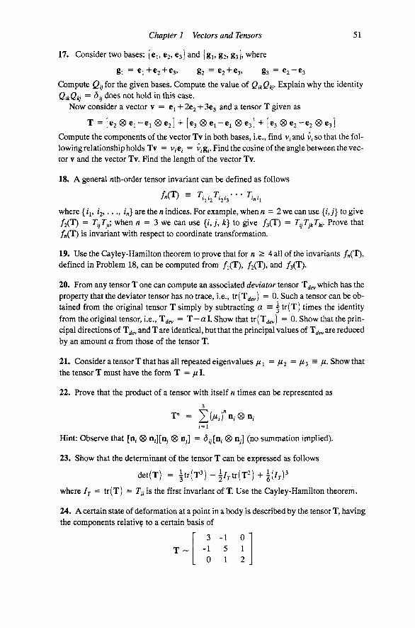
Chapter 1 Vectors and Tensors 51
17. Consider two bases: (ej, 62, 63) and jgi, g2, §3), where
gl = 61+62 + 63, g2 = 62 + 63, g3 = 6 2 - 6 3
Compute Qijior the given bases. Compute the value of QikQiq- Explain why the identity QikQiq = ^ij does not hold in this case.
Now consider a vector v = 61 + 262 + 363 and a tensor T given as
T = [62 0 61-61 0 6 2 ] + [63 (8)61-61 (8)63] + [63 0 62-62 0 6 3 ]
Compute the components of the vector Tv in both bases, i.e., find v, and v, so that the following relationship holds Tv = v,6, = v,g,. Find the cosine ofthe angle between the vector V and the vector Tv. Find the length of the vector Tv.
18. A general nth-order tensor invariant can be defined as follows
J"\ / 1*2 '23 "1
where {/j, (2,..., /„} are the n indices. For example, when n = 2wt can use {/,;} to give /2(T) = TijTjii when n = 3 we can use {/,;, k} to give fs(T) = TijTjJ^i' Prove that fn(T) is invariant with respect to coordinate transformation.
19. Use the Cayley-Hamilton theorem to prove that for « > 4 all of the invariants /n(T), defined in Problem 18, can be computed from /i(T), /2(T), and fsCT).
20. From any tensor T one can compute an associated deviator tensor T^^ which has the property that the deviator tensor has no trace, i.e., tr(T^^) = 0. Such a tensor can be obtained from the original tensor T simply by subtracting a = | tr(T) times the identity from the original tensor, i.e., T^ = T - a l . Show that tr(T^g^) = 0. Show that the principal directions of T^^and T are identical, but that the principal values of T^^ are reduced by an amount a from those of the tensor T.
21. Consider a tensor T that has all repeated eigenvalues /^i = /^2 ~ /^s ^ f^- Show that the tensor T must have the form T = jul.
22. Prove that the product of a tensor with itself n times can be represented as
Hint: Observe that [n, ® nj[ny ® n ] = ^y[n, ® n ] (no summation implied).
23. Show that the determinant of the tensor T can be expressed as follows
det(T) = i t r ( T 3 ) - i / , t r ( T ^ ) + i ( / , ) ^
where / j = tr(T) = T^ is the first invariant of T. Use the Cayley-Hamilton theorem.
24. A certain state of deformation at a point in a body is described by the tensor T, having the components relative to a certain basis of
3 - 1 0 -1 5 1 0 1 2

52 Fundamentals of Structural Mechanics
Find the eigenvalues and eigenvectors of T. Show that the invariants of the tensor T are the same in the given basis and in the basis defined by the eigenvectors for the present case.
25. Find the tensor T that has eigenvalues / = 1, / 2 = 2, and / 3 = 3 with two of the associated eigenvectors given by
n, = -^(61 + 62), n2 = | ( - 2 e i + 2e2 + e3)
Is the tensor unique (i.e., is there another one with these same eigenproperties)?
26. Find the tensor T that has eigenvalues // j = 1, //2 = 3, and / 3 = 3, with two of the associated eigenvectors given by
- | (ei + e2 + e3), n2 = j^y Hi = •^(ei + e2 + e3), n2 = -F(-e2 + e3)
Are the eigenvectors unique?
27. A certain state of deformation at a point in a body is described by the tensor T, having the components relative to a certain basis of
10-14 2 14 2 -1 -16
14 -16 5
Let the principal values and principal directions be designated as fi and n. Show that n = (-1, 2, 2) is a principal direction and find /^j . The second principal value is //j = 9 X 10"^, find n2. Find fi^ and n^ with as little computation as possible.
28. The equation for balance of angular momentum can be expressed in terms of a tensor T and the base vectors e as e, x (Te,) = 0 (sum on repeated index implied). What specific conditions must the components of the tensor T satisfy in order for this equation to be satisfied?
29. The tensor R that operates on vectors and reflects them (as in a mirror) with unit normal n is given by
R = I-2n(g)n
Compute the vector that results from [RR]v. Compute the length of the vector Rv in terms of the length of v. What is the inverse of the tensor R? Compute the eigenvalues and eigenvectors of R.
30. Let v(x) and u(x) be two vector fields, and T(x) be a tensor field. Compute the following expressions in terms of the components ( v„ w„ and T ) of these fields relative to the basis {ci, 62, 63): div(Tv), V(u • Tv), V(Tv), and u (g) Tv.
31. Evaluate the following expressions:
(a) div(div[x ® x]) (b) div(x div(xdivx)) (c) V[|| (V || x H ) f]
(d) div(x (8) div[x 0 x]) (e) V(xdivx) (f) V[x • V(x • x)]
where x = x^e^ +X2e2 + 363 is the position vector in space and all derivatives are with respect to the coordinates jc,.
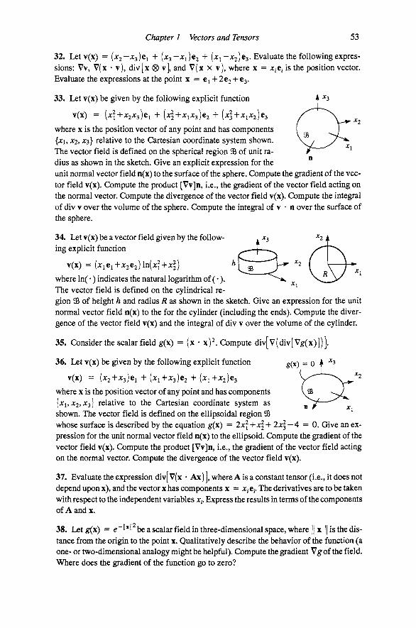
Chapter 1 Vectors and Tensors 53
32. Letv(x) = [x2-X2,)t^ + (•^3~^i)c2 + (JC^-0:2)63-Evaluate the following expressions: Vv, V(x • v), div [x ® v], and V(x x v), where x = jc,e, is the position vector. Evaluate the expressions at the point x = 61+262 + 63.
f \^x.
33. Let v(x) be given by the following explicit function
V(X) = [x\+X2X^)t^ + [x\+X^X^y2^ [4^^1X2)^3
where x is the position vector of any point and has components {xi, JC2, x^} relative to the Cartesian coordinate system shown. The vector field is defined on the spherical region 9& of unit radius as shown in the sketch. Give an explicit expression for the unit normal vector field n(x) to the surface of the sphere. Compute the gradient of the vector field v(x). Compute the product [Vv]n, i.e., the gradient of the vector field acting on the normal vector. Compute the divergence of the vector field v(x). Compute the integral of div V over the volume of the sphere. Compute the integral of v • n over the surface of the sphere.
34. Let v(x) be a vector field given by the following explicit function
v(x) = (xiCi+0:262) ln(^ + JC2) where ln( •) indicates the natural logarithm of (•). The vector field is defined on the cylindrical region S of height h and radius R as shown in the sketch. Give an expression for the unit normal vector field n(x) to the for the cylinder (including the ends). Compute the divergence of the vector field v(x) and the integral of div v over the volume of the cylinder.
35. Consider the scalar field g(x) = (x • x)^. Compute div[v(div[Vg(x)])].
36. Let v(x) be given by the following explicit function g(x) = 0
v(x) = (^^2+^3)61 + ^1+^^3)62 + ( 1+^=^2)63
where x is the position vector of any point and has components jxi,jC2, X3) relative to the Cartesian coordinate system as shown. The vector field is defined on the ellipsoidal region 3& whose surface is described by the equation g(\) = 2x\ +;c^ + 2J^ — A = 0. Give an expression for the unit normal vector field n(x) to the ellipsoid. Compute the gradient of the vector field v(x). Compute the product [Vv]n, i.e., the gradient of the vector field acting on the normal vector. Compute the divergence of the vector field v(x).
37. Evaluate the expression div[ V(x • Ax) ], where A is a constant tensor (i.e., it does not depend upon x), and the vector x has components x = JCJCJ. The derivatives are to be taken with respect to the independent variables jc . Express the results in terms of the components of A and x.
38. Let g(x) = e ~ll*'l be a scalar field in three-dimensional space, where || x || is the distance from the origin to the point x. Qualitatively describe the behavior of the function (a one- or two-dimensional analogy might be helpful). Compute the gradient Vgof the field. Where does the gradient of the function go to zero?
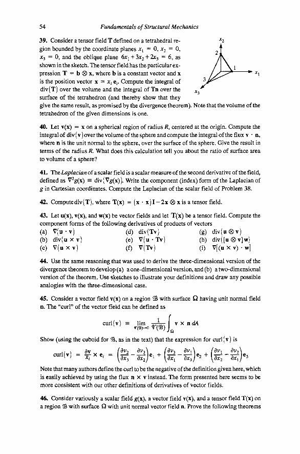
54 Fundamentals of Structural Mechanics
39. Consider a tensor field T defined on a tetrahedral region bounded by the coordinate planes x^ = 0,0^2 = 0, JC3 = 0, and the oblique plane 6x1 + 3x2 + 2x3 = 6, as shown in the sketch. The tensor field has the particular expression T = b ® X, where b is a constant vector and x is the position vector x = x, e,. Compute the integral of div(T) over the volume and the integral of Tn over the surface of the tetrahedron (and thereby show that they give the same result, as promised by the divergence theorem). Note that the volume of the tetrahedron of the given dimensions is one.
40. Let v(x) = X on a spherical region of radius R, centered at the origin. Compute the integral of div (v) over the volume of the sphere and compute the integral of the flux v • n, where n is the unit normal to the sphere, over the surface of the sphere. Give the result in terms of the radius R. What does this calculation tell you about the ratio of surface area to volume of a sphere?
41. The Laplacian of a scalar field is a scalar measure of the second derivative of the field, defined as V^g(x) = div( V^(x)). Write the component (index) form of the Laplacian of g in Cartesian coordinates. Compute the Laplacian of the scalar field of Problem 38.
42. Compute div (T), where T(x) = ( x - x ) I - 2 x ® x i s a tensor field.
43. Let u(x), v(x), and w(x) be vector fields and let T(x) be a tensor field. Compute the component forms of the following derivatives of products of vectors (a) V(u-v ) (d) div(Tv) (g) div(u(g)v) (b) div(u X v) (e) V(u • Tv) (h) div([u (g) v]w) (c) V ( u x v ) (f) V(Tv) (i) V [ ( u x v ) - w ]
44. Use the same reasoning that was used to derive the three-dimensional version of the divergence theorem to develop (a) a one-dimensional version, and (b) a two-dimensional version of the theorem. Use sketches to illustrate your definitions and draw any possible analogies with the three-dimensional case.
45. Consider a vector field v(x) on a region 35 with surface Q having unit normal field n. The "curl" of the vector field can be defined as
curl(v) = lim -^pr^ I y x ndA r(aa)-*o T(^) J
that the
„„W.f.e,.(g-g)...(S»-S|).,.(||-|g). Show (using the cuboid for % as in the text) that the expression for curl(v) is
Note that many authors define the curl to be the negative of the definition given here, which is easily achieved by using the flux n x v instead. The form presented here seems to be more consistent with our other definitions of derivatives of vector fields.
46. Consider variously a scalar field g(x), a vector field v(x), and a tensor field T(x) on a region 3& with surface Q with unit normal vector field n. Prove the following theorems
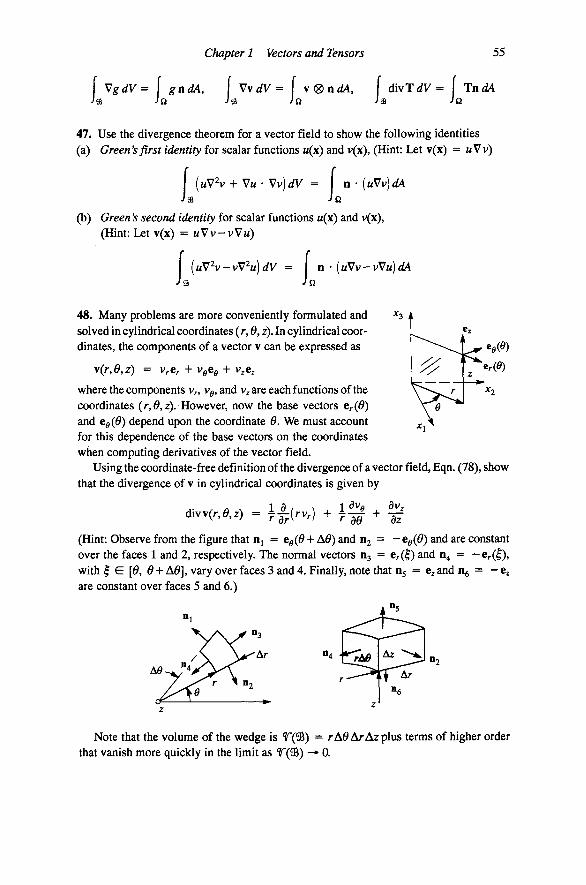
Chapter 1 Vectors and Tensors
[ Vg^y= [ gndA, [ VydV= [ y®ndA, f divTJy= [ TndA
55
47. Use the divergence theorem for a vector field to show the following identities (a) Green's first identity for scalar functions M(X) and v(x), (Hint: Let v(x) = wVv)
(wV v + V« • Vv)dV = n • [uVv)dA
(b) Green's second identity for scalar functions w(x) and v(x), (Hint: Let v(x) = wVv-vVw)
[uV\-vV'^u)dV = n • (wVv-vVw)d[A
48. Many problems are more conveniently formulated and - 3 4 solved in cylindrical coordinates (r, , z). In cylindrical coordinates, the components of a vector v can be expressed as
y{r,e,z) = v,e, + v e + v Cz
where the components V;., v , and v are each functions of the coordinates (r,^,z). However, now the base vectors ^r(&) and e^(^) depend upon the coordinate 0. We must account for this dependence of the base vectors on the coordinates when computing derivatives of the vector field.
Using the coordinate-free definition of the divergence of a vector field, Eqn. (78), show that the divergence of v in cylindrical coordinates is given by
divv(..,.) = ll:(.v.) . 1 ^ . S
(Hint: Observe from the figure that HJ = e^(^ + A^) and n2 = - e^(^) and are constant over the faces 1 and 2, respectively. The normal vectors n^ = er(^) and n4 = — e;.(|), with ^ E [6, 6 + AS], vary over faces 3 and 4. Finally, note that n^ = e and n^ = - e are constant over faces 5 and 6.)
rAB Az
Ar
Note that the volume of the wedge is ?'(S) = r A^ Ar Az plus terms of higher order that vanish more quickly in the limit as f (S) -* 0.