Vector Spaces in Physicsbland/courses/385/downloads/vector/vector.pdf · Vector Spaces in Physics...
187
San Francisco State University Department of Physics and Astronomy August 6, 2015 Vector Spaces in Physics Notes for Ph 385: Introduction to Theoretical Physics I R. Bland
Transcript of Vector Spaces in Physicsbland/courses/385/downloads/vector/vector.pdf · Vector Spaces in Physics...

San Francisco State University
Department of Physics and Astronomy
August 6, 2015
Vector Spaces in Physics
Notes
for
Ph 385: Introduction to
Theoretical Physics I
R. Bland
ii
TABLE OF CONTENTS
Chapter I. Vectors
A. The displacement vector.
B. Vector addition.
C. Vector products.
1. The scalar product.
2. The vector product.
D. Vectors in terms of components.
E. Algebraic properties of vectors.
1. Equality.
2. Vector Addition.
3. Multiplication of a vector by a scalar.
4. The zero vector.
5. The negative of a vector.
6. Subtraction of vectors.
7. Algebraic properties of vector addition.
F. Properties of a vector space.
G. Metric spaces and the scalar product.
1. The scalar product.
2. Definition of a metric space.
H. The vector product.
I. Dimensionality of a vector space and linear independence.
J. Components in a rotated coordinate system.
K. Other vector quantities.
Chapter 2. The special symbols ij and ijk, the Einstein summation
convention, and some group theory. A. The Kronecker delta symbol, ij
B. The Einstein summation convention.
C. The Levi-Civita totally antisymmetric tensor.
Groups.
The permutation group.
The Levi-Civita symbol.
D. The cross Product.
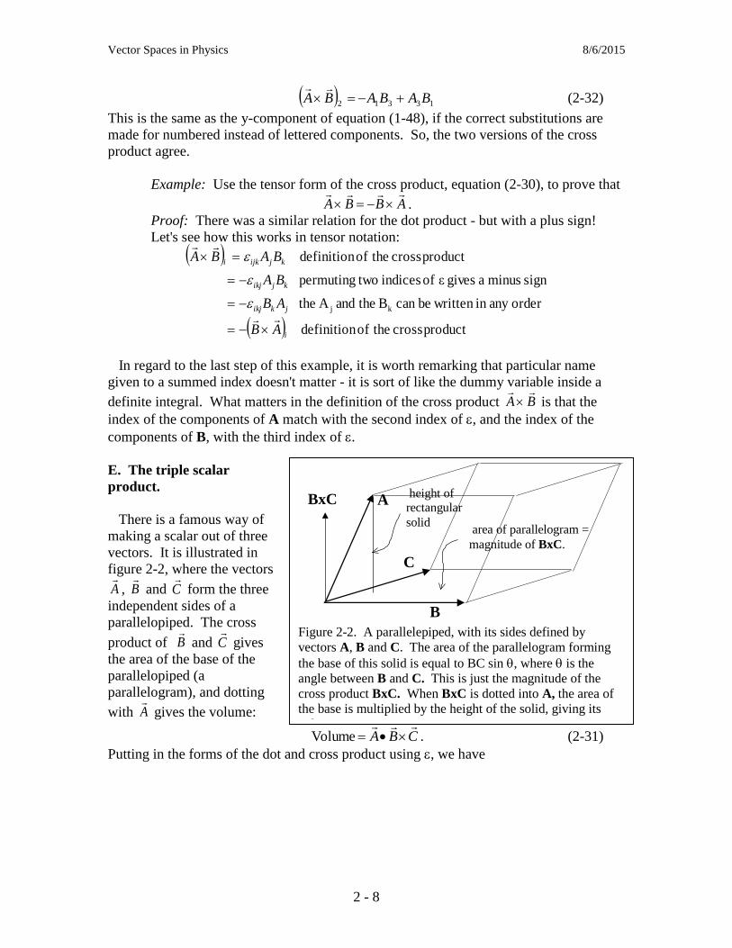
E. The triple scalar product.
F. The triple vector product.
The epsilon killer.
Chapter 3. Linear equations and matrices. A. Linear independence of vectors.
B. Definition of a matrix.
C. The transpose of a matrix.
D. The trace of a matrix.
E. Addition of matrices and multiplication of a matrix by a scalar.
F. Matrix multiplication.
G. Properties of matrix multiplication.
H. The unit matrix
I. Square matrices as members of a group.

iii
J. The determinant of a square matrix.
K. The 3x3 determinant expressed as a triple scalar product.
L. Other properties of determinants
Product law
Transpose law
Interchanging columns or rows
Equal rows or columns
M. Cramer's rule for simultaneous linear equations.
N. Condition for linear dependence.
O. Eigenvectors and eigenvalues
Chapter 4. Practical examples
A. Simple harmonic motion - a review
B. Coupled oscillations - masses and springs.
A system of two masses.
Three interconnected masses.
Systems of many coupled masses.
C. The triple pendulum
Chapter 5. The inverse; numerical methods
A. The inverse of a square matrix.
Definition of the inverse.
Use of the inverse to solve matrix equations.
The inverse matrix by the method of cofactors.
B. Time required for numerical calculations.
C. The Gauss-Jordan method for solving simultaneous linear equations.
D. The Gauss-Jordan method for inverting a matrix.
Chapter 6. Rotations and tensors A. Rotation of axes.
B. Some properties of rotation matrices.
Orthogonality
Determinant
C. The rotation group.
D. Tensors
E. Coordinate transformation of an operator on a vector space.
F. The conductivity tensor.
G. The inertia tensor.
Chapter 6a. Space-time four-vectors. A. The origins of special relativity.
B. Four-vectors and invariant proper time.
C. The Lorentz transformation.
D. Space-time events.
E. The time dilation.
F. The Lorentz contraction.
G. The Maxwell field tensor.

iv
Chapter 7. The Wave Equation A. Qualitative properties of waves on a string.
B. The wave equation.
Partial derivatives.
Wave velocity.
C. Sinusoidal solutions.
D. General traveling-wave solutions.
E. Energy carried by waves on a string.
Kinetic energy.
Potential energy.
F. The superposition principle.
G. Group and phase velocity.
Chapter 8. Standing Waves on a String
A. Boundary Conditions and Initial Conditions
String fixed at a boundary.
Boundary between two different strings.
B. Standing waves on a string.
Chapter 9. Fourier Series
A. The Fourier sine series.
The general solution.
Initial conditions.
Orthogonality.
Completeness.
B. The Fourier sine-cosine Series.
Odd and even functions.
Periodic functions in time.
C. The exponential Fourier series.
Chapter 10. Fourier Transforms and the Dirac Delta Function
A. The Fourier transform.
B. The Dirac delta function (x).
The rectangular delta function.
The Gaussian delta function.
Properties of the delta function.
C. Application of the Dirac delta function to Fourier transforms.
Basis states.
Functions of position x.
D. Relation to quantum mechanics.
Chapter 11. Maxwell's Equations in Special Relativity
Appendix A. Useful mathematical facts and formulae.
A. Complex numbers.
B. Some integrals and identities
C. The small-angle approximation.
D. Mathematical logical symbols.
Appendix B. Using the P&A Computer System 1. Logging on.
2. Running MatLab, Mathematica and IDL.
3. Mathematica.

v
Appendix C. Mathematica
1. Calculation of the vector sum using Mathematica.
2. Matrix operations in Mathematica
3. Speed test for Mathematica.
References
Vector Spaces in Physics 8/6/2015
1 - 1
Chapter 1. Vectors
We are all familiar with the distinction between things which have a direction and those
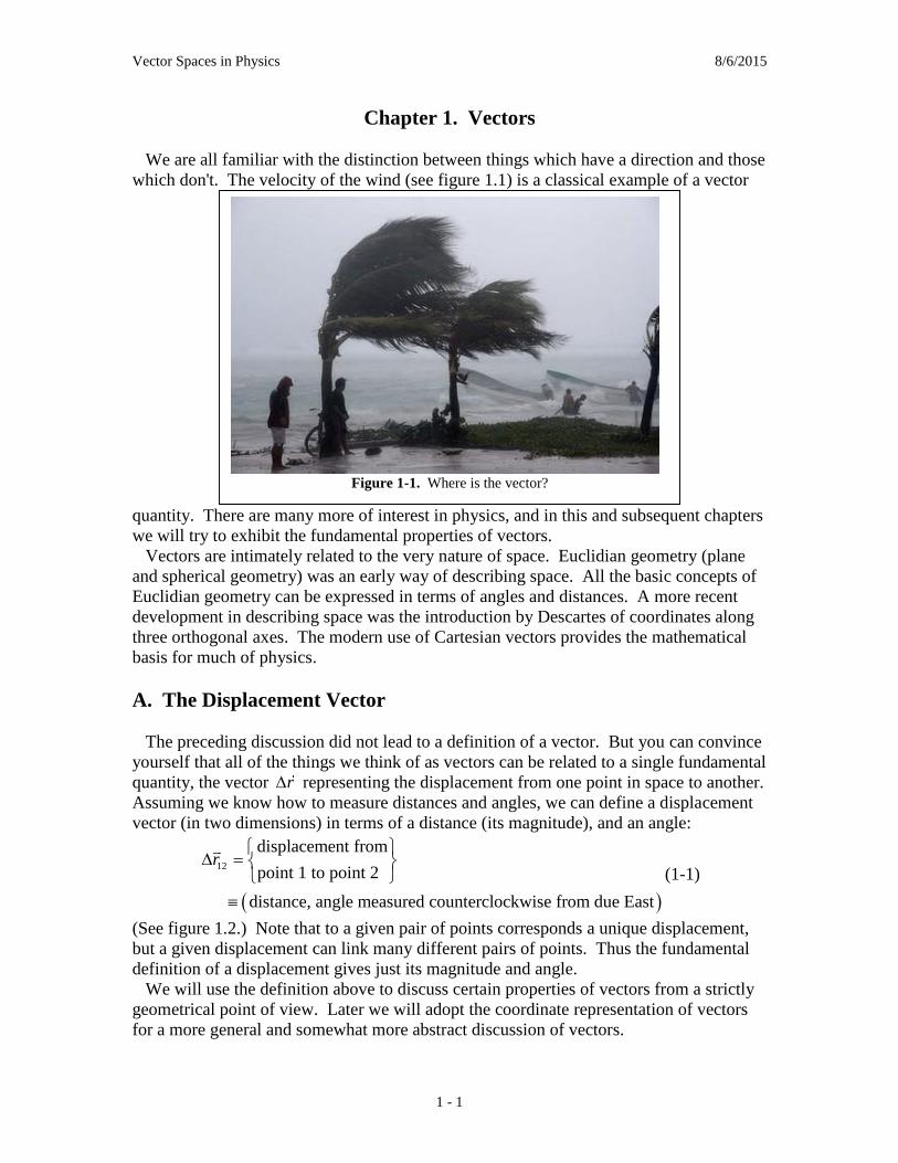
which don't. The velocity of the wind (see figure 1.1) is a classical example of a vector
quantity. There are many more of interest in physics, and in this and subsequent chapters
we will try to exhibit the fundamental properties of vectors.
Vectors are intimately related to the very nature of space. Euclidian geometry (plane
and spherical geometry) was an early way of describing space. All the basic concepts of
Euclidian geometry can be expressed in terms of angles and distances. A more recent
development in describing space was the introduction by Descartes of coordinates along
three orthogonal axes. The modern use of Cartesian vectors provides the mathematical
basis for much of physics.
A. The Displacement Vector
The preceding discussion did not lead to a definition of a vector. But you can convince
yourself that all of the things we think of as vectors can be related to a single fundamental
quantity, the vector r representing the displacement from one point in space to another.
Assuming we know how to measure distances and angles, we can define a displacement
vector (in two dimensions) in terms of a distance (its magnitude), and an angle:
12
displacement from
point 1 to point 2
distance, angle measured counterclockwise from due East
r
(1-1)
(See figure 1.2.) Note that to a given pair of points corresponds a unique displacement,
but a given displacement can link many different pairs of points. Thus the fundamental
definition of a displacement gives just its magnitude and angle.
We will use the definition above to discuss certain properties of vectors from a strictly
geometrical point of view. Later we will adopt the coordinate representation of vectors
for a more general and somewhat more abstract discussion of vectors.
Figure 1-1. Where is the vector?

Vector Spaces in Physics 8/6/2015
1 - 2
B. Vector Addition
A quantity related to the displacement vector is the position vector for a point.
Positions are not absolute – they must be measured relative to a reference point. If we
call this point O (the "origin"), then the position vector for point P can be defined as
follows:
displacement from point O to point PPr (1-2)
It seems reasonable that the displacement from point 1 to point 2 should be expressed in
terms of the position vectors for 1 and 2. We are be tempted to write
1212 rrr
(1-3)
A "difference law" like this is certainly valid for temperatures, or even for distances along
a road, if 1 and 2 are two points on the road. But what does subtraction mean for
vectors? Do you subtract the lengths and angles, or what? When are two vectors equal?
In order to answer these questions we need to systematically develop the algebraic
properties of vectors.
We will let A
, B
, C
, etc. represent vectors. For the moment, the only vector
quantities we have defined are displacements in space. Other vector quantities which we
will define later will obey the same rules.
Definition of Vector Addition. The sum of two vector displacements can be defined so
as to agree with our intuitive notions of displacements in space. We will define the sum
of two displacements as the single displacement which has the same effect as carrying out
the two individual displacements, one after the other. To use this definition, we need to
be able to calculate the magnitude and angle of the sum vector. This is straightforward
using the laws of plane geometry. (The laws of geometry become more complicated in
three dimensions, where the coordinate representation is more convenient.)
Let A
and B
be two displacement vectors, each defined by giving its length and angle:
).,(
),,(
B
A
BB
AA
(1-4)
point
1
point
2
r
east
angle
distance
Figure 1-2. A vector, specified by giving a distance and an angle.

Vector Spaces in Physics 8/6/2015
1 - 3
Here we follow the convention of using the quantity A (without an arrow over it) to
represent the magnitude of A
; and, as stated above, angles are measured
counterclockwise from the easterly direction. Now imagine points 1, 2, and 3 such that
A
represents the displacement from 1 to 2, and B
represents the displacement from 2 to
3. This is illustrated in figure 1-3.
Definition: The sum of two given displacements A
and B
is the third
displacement C
which has the same effect as making displacements A
and
B
in succession.
It is clear that the sum C
exists, and we know how to find it. An example is shown in
figure 1-4 with two given vectors A
and B
and their sum C
. It is fairly clear that the
length and angle of C
can be determined (using trigonometry), since for the triangle 1-2-
3, two sides and the included angle are known. The example below illustrates this
calculation.
Example: Let A
and B
be the two vectors shown in figure 1-4: A
=(10 m,
48), B
=(14 m, 20). Determine the magnitude and angle from due east of their
sum C
, where BAC
. The angle opposite side C can be calculated as
shown in figure 1-4; the result is that 2 = 152. Then the length of side C can be
calculated from the law of
A
B
1
2
3
A
B
Figure 1-3. Successive displacements A
and B
.

Vector Spaces in Physics 8/6/2015
1 - 4
cosines:
C2 = A2 + B2 -2AB cos 2
giving
C = [(10 m)2 + (14 m)2 - 2(10m)(14m)cos 152]1/2
= 23.3072 m .
The angle 1 can be calculated from the law of sines:
sin 1 / B = sin 2 / C
giving
1 = sin-1 .28200
= 16.380 .
The angle C is then equal to 48 - 1 = 31.620 . The result is thus
23.3072 m, 31.620C .
One conclusion to be drawn from the previous example is that calculations using the
geometrical representation of vectors can be complicated and tedious. We will soon see
that the component representation for vectors simplifies things a great deal.
C. Product of Two Vectors
Multiplying two scalars together is a familiar and useful operation. Can we do the
same thing with vectors? Vectors are more complicated than scalars, but there are two
useful ways of defining a vector product.
The Scalar Product. The scalar product, or dot product, combines two vectors to give a
scalar:
)-(c ABosBABA
(1-5)
48
20
1
2
3
A
B
C
10 m
14 m
C
BAC
1
3
2
48
20
1
2
3
48-20
= 28
180-28
= 152
Figure 1-4. Example of vector addition. Each vector's direction is measured counterclockwise from due
East. Vector A
is a displacement of 10 m at an angle of 48and vector B
is a displacement of 14 m at an
angle of 20.

Vector Spaces in Physics 8/6/2015
1 - 5
This simple definition is illustrated in figure
1-5. One special property of the dot product
is its relation to the length A of a vector A
:
2AAA
(1-6)
This in fact can be taken as the definition of
the length, or magnitude, A.
An interesting and useful type of vector is a
unit vector, defined as a vector of length 1.
We usually write the symbol for a unit vector
with a hat over it instead of a vector symbol:
u . Unit vectors always have the property
1ˆˆ uu (1-7)
Another use of the dot product is to define orthogonality of two vectors. If the angle
between the two vectors is 90, they are usually said to be perpendicular, or orthogonal.
Since the cosine of 90 is equal to zero, we can equally well define orthogonality of two
vectors using the dot product:
0A B A B (1-8)
Example. One use of the scalar product in physics is in calculating the work
done by a force F
acting on a body while it is displaced by the vector
displacement d
. The work done depends on the distance moved, but in a special
way which projects out the distance moved in the direction of the force:
Work F d (1-9)
Similarly, the power produced by the motion of an applied force F
whose point
of application is moving with velocity v is given by
Power F v (1-10)
In both of these cases, two vectors are combined to produce a scalar.
Example. To find the component of a vector A in a direction given by the unit
vector n , take the dot product of the two vectors.
ˆComponent of along A n A n (1-11)
The Vector Product. The vector product, or cross product, is considerably more
complicated than the scalar product. It involves the concept of left and right, which has
an interesting history in physics. Suppose you are trying to explain to someone on a
distant planet which side of the road we drive on in the USA, so that they could build a
car, bring it to San Francisco and drive around. Until the 1930's, it was thought that there
was no way to do this without referring to specific objects which we arbitrarily designate
as left-handed or right-handed. Then it was shown, by Madame Wu, that both the
electron and the neutrino are intrinsically left-handed! This permits us to tell the alien
how to determine which is her right hand. "Put a sample of 60Co nuclei in front of you,
on a mount where it can rotate freely about a vertical axis. Orient the nuclei in a
A
B
B - A
Figure 1-5. Vectors A
and B
. Their dot
product is equal to A B cos(B - A).
Their cross product BA
has magnitude
A B sin(B - A), directed out of the paper.

Vector Spaces in Physics 8/6/2015
1 - 6
magnetic field until the majority of the decay electrons go downwards. The sample will
gradually start to rotate so that the edge nearest you moves to the right. This is said to be
a right-handed rotation about the vertically upward axis." The reason this works is that
the magnetic field aligns the cobalt nuclei vertically, and the subsequent nuclear decays
emit electrons preferentially in the opposite direction to the nuclear spin. (Cobalt-60
decays into nickel-60 plus an electron and an anti-electron neutrino,
60 60
eCo Ni e ν (1-12)
See the Feynman Lectures for more information on this subject.) Now you can just tell
the alien, "We drive on the right." (Hope she doesn't land in Australia.)
This lets us define the cross product of two vectors A
and B
as shown in figure 1-5.
The cross product of these two vectors is a third vector C
, with magnitude
C = |A B sin (B - A)|, (1-13)
perpendicular to the plane containing A
and B
, and in the sense "determined by the
right-hand rule." This last phrase, in quotes, is shorthand for the following operational
definition: Place A
and B
so that they both start at the same point. Choose a third
direction perpendicular to both A
and B
(so far, there are two choices), and call it the
upward direction. If, as A
rotates towards B
, it rotates in a right-handed direction, then
this third direction is the direction of C
.
Example. The Lorentz Force is the force exerted on a charged particle due to
electric and magnetic fields. If the particle's charge is given by q and it is moving
with velocity v , in electric field E and magnetic field B , the force F is given
by
F qE qv B (1-14)
The second term is an example of a vector quantity created from two other
vectors.
A
B
BA
x
y
z
Figure 1-6. Illustration of a cross product. Can you prove that if A
is along the x-
axis, then BA
is in the y-z plane?

Vector Spaces in Physics 8/6/2015
1 - 7
Example. The cross product is used to find the direction of the third axis in a
three-dimensional space. Let u and v be two orthogonal unit vectors,
representing the first (or x) axis and the second (or y) axis, respectively. A unit
vector w in the correct direction for the third (or z) axis of a right-handed
coordinate system is found using the cross product:
ˆ ˆ ˆw u v (1-15)
D. Vectors in Terms of Components
Until now we have discussed vectors from a purely geometrical point of view. There is
another representation, in terms of components, which makes both theoretical analysis
and practical calculations easier. It is a fact about the space that we live in that it is
possible to find three, and no more than three, vectors that are mutually orthogonal. (This
is the basis for calling our space three dimensional.) Descartes first introduced the idea
of measuring position in space by giving a distance along each of three such vectors. A
Cartesian coordinate system is determined by a particular choice of these three vectors.
In addition to requiring the vectors to be mutually orthogonal, it is convenient to take
each one to have unit length.
A set of three unit vectors defining a Cartesian coordinate system can be chosen as
follows. Start with a unit vector i in any direction you like. Then choose any second
unit vector j which is perpendicular to i . As the third unit vector, take jik ˆˆˆ .
These three unit vectors )ˆ,ˆ,ˆ( kji are said to be orthonormal. This means that they are
mutually orthogonal, and normalized so as to be unit vectors. We will often refer to their
directions as the x, y, and z directions. We will also sometimes refer to the three vectors
as )ˆ,ˆ,ˆ( 321 eee , especially when we start writing sums over the three directions.
Suppose that we have a vector A
and three orthogonal unit vectors )ˆ,ˆ,ˆ( kji , all defined
as in the previous sections by their length and direction. The three unit vectors can be
used to define vector components of A
, as follows:
.ˆ
,ˆ
,ˆ
kAA
jAA
iAA
z
y
x
(1-16)
This suggests that we can start a discussion of vectors from a component view, by simply
defining vectors as triplets of scalar numbers:
x
y
z
A
A A
A
Component Representation of Vectors (1-17)
It remains to prove that this definition is completely equivalent to the geometrical
definition, and to define vector addition and multiplication of a vector by a scalar in terms
of components.

Vector Spaces in Physics 8/6/2015
1 - 8
Let us show that these two ways of specifying a vector are equivalent - that is, to each
geometrical vector (magnitude and direction) there corresponds a single set of
components, and (conversely) to each set of components there corresponds a single
geometrical vector. The first assertion follows from the relation (1-16), showing how to
determine the triplet of components for any given geometrical vector. The dot product of
any two vectors exists, and is unique.
The converse is demonstrated in Figure 1-7. It is seen that the vector A
can be written as
the sum of three vectors proportional to its three components:
zyx AkAjAiA ˆˆˆ
(1-18)
From the diagram it is clear that, given three components, there is just one such sum. So,
we have established the equivalence
( , )
x
y
z
A
A magnitude direction A
A
(1-19)
E. Algebraic Properties of Vectors.
As a warm-up, consider the familiar algebraic properties of scalars. This provides a road
map for defining the analogous properties for vectors.
Equality.
x
y
z
xAi
yAj
zAk
Figure 1-7. Illustration of the addition of the component vectors iAx, jAy, and kAz to get the vector A
.
This proves that a given set of values for (Ax, Ay, Az) leads to a unique vector A
in the geometrical picture.

Vector Spaces in Physics 8/6/2015
1 - 9
and
a b b a
a b b c a c
Addition and multiplication of scalars.
( ) ( )
( ) ( )
( )
a b b a
a b c a b c a b c
ab ba
a bc ab c abc
a b c ab ac
Zero, negative numbers.
0
( ) 0
a a
a a
No surprises there.
Equality. We will say that two vectors are equal, meaning that they are really the same
vector, if all three of their components are equal:
, , .x x y y z zA B A B A B A B (1-20)
The commutative property, A B B A , and the transitive property,
and A B B C A C follow immediately, since components are scalars.
Vector Addition. We will adopt the obvious definition of vector addition using
components:
zzz
yyy
xxx
BAC
BAC
BAC
BAC
DEFINITION (1-21)
That is to say, the components of the sum are the sums of the components of the vectors
being added. It is necessary to show that this is in fact the same definition as the one we
introduced for geometrical vectors. This can be seen from the geometrical construction
shown in figure 1-7a.
Vector Spaces in Physics 8/6/2015
1 - 10
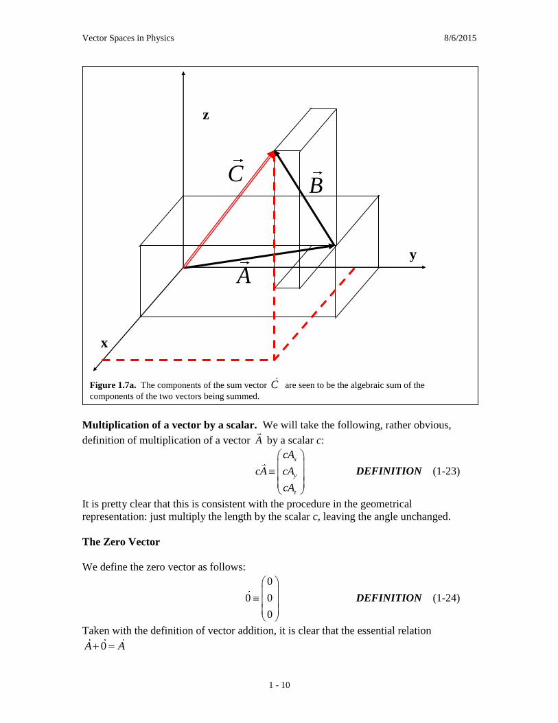
Multiplication of a vector by a scalar. We will take the following, rather obvious,
definition of multiplication of a vector A
by a scalar c:
x
y
z
cA
cA cA
cA
DEFINITION (1-23)
It is pretty clear that this is consistent with the procedure in the geometrical
representation: just multiply the length by the scalar c, leaving the angle unchanged.
The Zero Vector
We define the zero vector as follows:
0
0 0
0
DEFINITION (1-24)
Taken with the definition of vector addition, it is clear that the essential relation
0A A
y
z
x
A
B C
Figure 1.7a. The components of the sum vector C are seen to be the algebraic sum of the
components of the two vectors being summed.
Vector Spaces in Physics 8/6/2015
1 - 11
is satisfied. And a vector with all zero-length components certainly fills the bill as the
geometrical version of the zero vector.
The Negative of a Vector. The negative of a vector in terms of components is also easy
to guess:
x
y
z
A
A A
A
DEFINITION (1-26)
The essential relation 0A A will clearly be satisfied, in terms of components. It is
also easy to prove that this corresponds to the geometrical vector with the direction
reversed; we will also omit this proof.
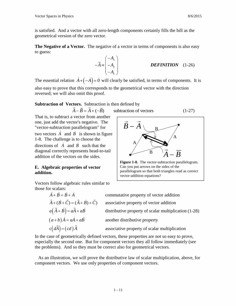
Subtraction of Vectors. Subtraction is then defined by
( ) subtraction of vectorsA B A B (1-27)
That is, to subtract a vector from another
one, just add the vector's negative. The
"vector-subtraction parallelogram" for
two vectors A and B is shown in figure
1-8. The challenge is to choose the
directions of A and B such that the
diagonal correctly represents head-to-tail
addition of the vectors on the sides.
E. Algebraic properties of vector
addition.
Vectors follow algebraic rules similar to
those for scalars:
commutative property of vector addition
( ) ( ) ) associative property of vector addition
distributive property of scalar multiplication
another
A B B A
A B C A B C
a A B aA aB
a b A aA aB
distributive property
c associative property of scalar multiplicationdA cd A
(1-28)
In the case of geometrically defined vectors, these properties are not so easy to prove,
especially the second one. But for component vectors they all follow immediately (see
the problems). And so they must be correct also for geometrical vectors.
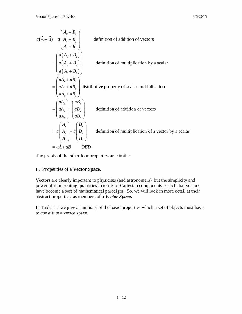
As an illustration, we will prove the distributive law of scalar multiplication, above, for
component vectors. We use only properties of component vectors.
AB
A
A
B
B BA
Figure 1-8. The vector-subtraction parallelogram.
Can you put arrows on the sides of the
parallelogram so that both triangles read as correct
vector-addition equations?
Vector Spaces in Physics 8/6/2015
1 - 12
( ) definition of addition of vectors
definition of multiplication by a scalar
distributive property of scalar
x x
y y
z z
x x
y y
z z
x x
y y
z z
A B
a A B a A B
A B
a A B
a A B
a A B
aA aB
aA aB
aA aB
multiplication
definition of addition of vectors
definition of multiplication of a vector by a scalar
x x
y y
z z
x x
y y
z z
aA aB
aA aB
aA aB
A B
a A a B
A B
aA aB QED
The proofs of the other four properties are similar.
F. Properties of a Vector Space.
Vectors are clearly important to physicists (and astronomers), but the simplicity and
power of representing quantities in terms of Cartesian components is such that vectors
have become a sort of mathematical paradigm. So, we will look in more detail at their
abstract properties, as members of a Vector Space.
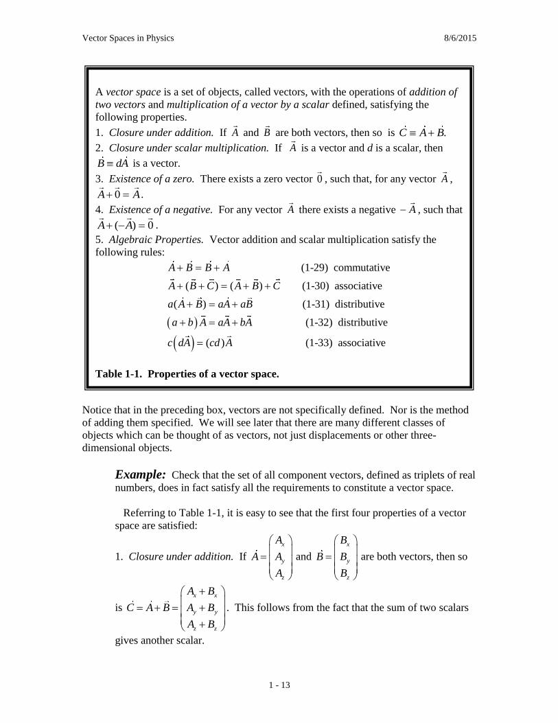
In Table 1-1 we give a summary of the basic properties which a set of objects must have
to constitute a vector space.
Vector Spaces in Physics 8/6/2015
1 - 13
Notice that in the preceding box, vectors are not specifically defined. Nor is the method
of adding them specified. We will see later that there are many different classes of
objects which can be thought of as vectors, not just displacements or other three-
dimensional objects.
Example: Check that the set of all component vectors, defined as triplets of real
numbers, does in fact satisfy all the requirements to constitute a vector space.
Referring to Table 1-1, it is easy to see that the first four properties of a vector
space are satisfied:
1. Closure under addition. If
x
y
z
A
A A
A
and
x
y
z
B
B B
B
are both vectors, then so
is
x x
y y
z z
A B
C A B A B
A B
. This follows from the fact that the sum of two scalars
gives another scalar.
A vector space is a set of objects, called vectors, with the operations of addition of
two vectors and multiplication of a vector by a scalar defined, satisfying the
following properties.
1. Closure under addition. If A
and B
are both vectors, then so is .C A B
2. Closure under scalar multiplication. If A
is a vector and d is a scalar, then
B dA is a vector.
3. Existence of a zero. There exists a zero vector 0
, such that, for any vector A
,
AA
0 .
4. Existence of a negative. For any vector A
there exists a negative A
, such that
0)(
AA .
5. Algebraic Properties. Vector addition and scalar multiplication satisfy the
following rules:
(1-29) commutative
( ) ( ) (1-30) associative
( ) (1-31) distributive
(1-32) distr
A B B A
A B C A B C
a A B aA aB
a b A aA bA
ibutive
( ) (1-33) associativec dA cd A
Table 1-1. Properties of a vector space.
Vector Spaces in Physics 8/6/2015
1 - 14
2. Closure under multiplication. If A
is a vector and d is a scalar, then
x
y
z
dA
B dA dA
dA
is a vector. This follows from the fact that the product of two
scalars gives another scalar.
3. Zero. There exists a zero vector
0
0 0
0
, such that, for any vector A
,
0
0 0
0
x x
y y
z z
A
A A A
A
. This follows from the addition-of-zero property for
scalars.
4. Negative. For any vector A
there exists a negative
x
y
z
A
A A
A
, such that
0)(
AA . Adding components gives zero for the components of the sum.
5. The algebraic properties (1-29) through (1-33) were discussed above;
they are satisfied for component vectors.
So, all the requirements for a vector space are satisfied by component vectors.
This had better be true! The whole point of vector spaces is to generalize from
component vectors in three-dimensional space to a broader category of
mathematical objects that are very useful in physics.
Example: The properties above have clearly been chosen so that the usual
definition of vectors, including how to add them, satisfies these conditions. But
the concept of a vector space is intended to be more general. What if we define
vectors in two dimensions geometrically (having a magnitude and an angle) and
we keep multiplication by a scalar the same, but we redefine vector addition in the
following way.
( , )A BC A B A B (1-34)
This might look sort of reasonable, if you didn't know better. Which of the
properties (1)-(5) in Table 1-1 are satisfied?
1. Closure under addition: OK. A + B is an acceptable magnitude, and A +
B is an acceptable angle. (Angles greater than 360 are wrapped around.)
2. Closure under scalar multiplication: OK
3. Zero: the vector 0 (0,0) works fine; adding it on doesn't change A .
4. Negative: Not OK. There is no way to add two positive magnitudes
(magnitudes are non-negative) to get zero.
5. Algebraic properties: You can easily show that these are all satisfied.
Vector Spaces in Physics 8/6/2015
1 - 15
Conclusion: With this definition of vector addition, this is not a vector space.
G. Metric Spaces and the Scalar Product
The vector space as we have just defined it lacks something important. Thinking of
displacements, the length of a displacement, measuring the distance between two points,
is essential to describing space. So we want to add a way of assigning a magnitude to a
vector. This is provided by the scalar product.
The scalar product. The components of two vectors can be combined to give a scalar as
follows:
zzyyxx BABABABA
DEFINITION (1-40)
It is easy to show that the result follows from the representation of A
and B
in terms of
the three unit vectors of the Cartesian coordinate system:
zzyyxx
zyxzyx
BABABA
BkBjBiAkAjAiBA
)ˆˆˆ()ˆˆˆ(
where we have used the orthonormality of the unit vectors, 1ˆˆˆˆˆˆ kkjjii ,
0ˆˆˆˆˆˆ kjkiji . From the above definition in terms of components, it is easy to
demonstrate the following algebraic properties for the scalar product:
1-13
1-14
1-15
A B B A
A B C A B A C
A aB a A B
The inner product of a displacement with itself can then be used to define a distance
between points 1 and 2:
2 2 2
12 12 12 12 12 12r r r x y z (1-41)
From this expression we see that the distance between two points will not be zero unless
they are in fact the same point.
The scalar product can be used to define the direction cosines of an arbitrary vector,
with respect to a set of Cartesian coordinate axes. The direction cosines are defined as
follows (see figure 1-9):
DIRECTION COSINES , , and of a vector A
(1-42)

Vector Spaces in Physics 8/6/2015
1 - 16
A
AkA
A
A
AjA
A
A
AiA
A
z
y
x
ˆ1cos
ˆ1cos
ˆ1cos
Specifying these three values is one way of
giving the direction of a vector. However,
only two angles are required to specify a
direction in space, so these three angles must
not be independent. It can be shown (see
problems) that
1coscoscos 222
(1-43)
Definition of a Metric Space. The properties given in table 1-1 constitute the standard
definition of a vector space. However, inclusion of a scalar product turns a vector space
into the much more useful metric space, as defined in table 1-2. The difference between
a vector space and a metric space is the concept of distance introduced by the inner
product.
H. The vector product.
The geometrical definition of the cross product of A
and B
results in a third vector, say,
C
. The relation between A
, B
and is C
quite complicated, involving the idea of right-
handedness vs. left-handedness. We have already built a handedness into our coordinate
system in the way we choose the third unit vector, jik ˆˆˆ . As a preliminary to
A metric space is defined as a vector space with, in addition to its usual properties,
an inner product defined which has the following properties:
1. If A
and B
are vectors, then the inner product A B is a scalar.
2. 0A A 0
A . (1-44)
3. The following algebraic properties of the inner product must be obeyed:
A B B A
A B C A B A C
A aB a A B
(1-45)
Table 1-2. Properties of a metric space. Note that the scalar product of two
vectors as just defined has all of these properties.
A
x
y
z
Figure 1-9. The direction cosines for the vector
A are the cosines of the three angles shown.

Vector Spaces in Physics 8/6/2015
1 - 17
evaluating the cross product BA
, we work out the various cross products among the
unit vectors kji ˆ,ˆ,ˆ . From equation (1-17) we see that the cross product of two
perpendicular unit vectors has magnitude 1. We use the right-hand rule and refer to
figure 1-11 to get the direction of the cross products. This gives
jki
ijk
kij
jik
ikj
kji
ˆˆ
ˆˆˆ
ˆˆˆ
ˆˆˆ
ˆˆˆ
ˆˆˆ
(1-46)
Now it is straight forward to evaluate BA
in terms of components:
;ˆˆˆˆˆˆ
ˆˆˆˆˆˆ
iBAjBAiBAkBAjBAkBA
BkBjBiAkAjAiBA
yzxzzyxyzxyx
zyxzyx
(1-47)
This is not as hard to memorize as you might think - stare at it for a while and notice
permutation patterns (yz vs. zy, etc.) Later on we will have some other, even more
elegant ways of writing the cross product.
The cross product is used to represent a number of interesting physical quantities - for
example, the torque, Fr
, and the magnetic force, BvqF
, to name just a
couple.
The cross product satisfies the following algebraic properties:
(1-48)
( ) (1-49)
( ) ( ) (1-50)
A B B A
A B C A C B C
A aB a A B
Note that the order matters; the cross product is not commutative.
I. Dimensionality of a vector space and linear independence.
In constructing our coordinate system we used a very specific procedure for choosing the
directions of the axes, which only works for 3 dimensions. There is a broader, general
question to be asked about any vector space: What is the minimum number of vectors
required to "represent" all the others? This minimum number n is the dimensionality of a
vector space.
ˆ( )
ˆ( )
ˆ( )
y z z y
z x x z
x y y x
A B i A B A B
j A B A B
k A B A B
definition of the cross product

Vector Spaces in Physics 8/6/2015
1 - 18
Here is a more precise definition of dimensionality. Consider vectors 1E
, 2E
, . . . mE
.
These vectors are said to be linearly dependent if there exist constants (scalars) c1, c2, . . .
cm, not all zero, such that
0...2211
mm EcEcEc . (1-51)
If it is not possible to find such
constants ci, then the m vectors are
said to be linearly independent.
Now imagine searching among all
the vectors in the space to find the
largest group of linearly
independent vectors. The
dimensionality n of a vector space
is the largest number of linearly
independent vectors which can be found in the space.*
Example using geometrical vectors. Consider the three vectors shown in figure 1-
10. Which of the pairs BA
, , CA
, , and CB
, are linearly independent?
Solution: It is pretty clear that 0
CAa , for some value of a about equal to 2;
so A
and C
are not linearly independent. But A
and B
do not add up to zero no matter
what scale factors are used. To see this more clearly, suppose that there exist a and b
such that 0
BbAa ; then one can solve for B
, giving Ab
aB
. This means that
A
and B
are in the same direction, and this is clearly not so, showing by contradiction
that A
and B
are not linearly dependent. A similar line of reasoning applies to B
and
C
. Conclusion: BA
, and CB
, are the possible choices of two linearly independent
vectors.
Example using coordinates. Consider the three vectors
1 2 3
2 4 3
1 , 3 , 2 .
1 3 1
E E E
(1-52)
Are they linearly independent?
Solution: Try to find c1, c2, and c3 such that
* This may sound a bit vague. Suppose you look high and low and you can only find at most two linearly
independent displacement vectors. Are you sure that the dimensionality of your space is two? What if you
just haven't found the vectors representing the third dimension (or the fourth dimension!) This is the
subject of the short film Flatland.
x
y
A C
B
Figure 1-10. Three vectors in a plane.
Vector Spaces in Physics 8/6/2015
1 - 19
0332211
EcEcEc . (1-53)
This means that the sums of x-components, y-components and z-components must
separately add up to zero, giving three equations:
component-z 03
component-y 023
component x0342
321
321
321
ccc
ccc
ccc
.
Now we solve for c1, c2, and c3. Subtracting the third equation from the second gives c3
=0. The first and second equations then become
03
042
21
21
cc
cc.
The first equation gives c1 = -2c2, and the second equation gives c1 = -3c2. The only
consistent solution is c1 = c2 = c3 = 0. These three vectors are linearly independent!
This second example is a little messier and less satisfying than the previous example, and
it is clear that in 4, 5 or more dimensions the process would be difficult. In chapter 2 we
will discuss more elegant and powerful methods for solving simultaneous linear
equations.
Solving simultaneous linear equations with Mathematica. It is hard to resist
asking Mathematica to do this problem. Here is how you do it:
Solve[{2c1+4c2+3c3==0,c1+3c2+2c3==0,c1+3c2+c3==0},{c2,c3}] {}
This is Mathematica’s way of telling us that there is no solution.
What if we try to make 1E
, 2E
, and 3E
linearly dependent? If we change 2E
to
4
3
1
,
then the sum of 1E
and 2E
is twice 3E
, so the linear dependence relation
02 321
EEE
should be satisfied; this corresponds to c2 = c1, c3 = -2c1. Let’s ask Mathematica:
Solve[{2c1+4c2+3c3==0,c1+3c2+2c3==0,c1+c2+c3==0},{c2,c3}] {{c2->c1,c3->-2 c1}}
Sure enough!!
Is this cheating? I don't think so!

Vector Spaces in Physics 8/6/2015
1 - 20
J. Components in a Rotated Coordinate System. In physics there are lots of reasons
for changing from one coordinate system to another. Usually we try to work only with
coordinate systems defined by orthonormal unit vectors. Even so, the coordinates of a
vector fixed in space are different from one such coordinate system to another. As an
example, consider the vector A
shown in figure 1-11.
It has components Ax and Ay, relative to the x and y axes. But, relative to the x' and y'
axes, it has different components Ax' and Ay'. You can perhaps see from the complicated
construction in figure 2-3 that
Ax'=Ax cos + Ay sin (1-54)
And a similar construction leads to
Ay'=-Ax sin + Ay cos (1-55)
There is another, easier (algebraic rather than geometrical) way to obtain this result:
'ˆˆ'ˆˆ
'ˆ)ˆˆ(
'ˆ'
ijAiiA
iAjAi
iAA
yx
yx
x
,
'ˆˆ'ˆˆ
'ˆ)ˆˆ(
'ˆ'
jjAjiA
jAjAi
jAA
yx
yx
y
,
We can evaluate the dot products between unit vectors
with the aid of figure 1-12, with the result
x
y
A
Ax
x'
y'
Ay
Ax'
Ax cos
Ay sin
Figure 1-11. Coordinates of a vector A
in two different coordinate systems.
i
i'
jj'
Figure 1-12. Unit vectors for
unrotated (i and j) and rotated
(i' and j') coordinate systems.

Vector Spaces in Physics 8/6/2015
1 - 21
cos'ˆˆ
,sin)2
cos('ˆˆ
sin)2
cos('ˆˆ
,cos'ˆˆ
jj
ij
ji
ii
, (1-57)
This gives for the transformation from unprimed to primed coordinates
cossin'
sincos'
yxy
yxx
AAA
AAA
, (1-58)
It is easy to generalize this procedure to three or more dimensions. However, we will
wait to do this until we have introduced some more powerful notation, in the next
chapter.
K. Other Vector Quantities
You may wonder, "What happened to all the other vectors in physics, like velocity,
acceleration, force, . . . ?" They can ALL be derived from the displacement vector, by
taking derivatives or by using a law such as Newton's 2nd law. For example, the average
velocity of a migrating duck which flies from point 1 to point 2 in time t is equal to
)(1
1212 rrt
v
(1-40)
The quantity )( 12 rr
, is the sum of two vectors (the vector 1r
and the vector 2r
, which
is the negative of the vector 2r
), and so )( 12 rr
is itself a vector. It is multiplied by a
scalar, the quantity t
1. And the product of a vector and a scalar is a vector. So, average
velocities are vector quantities. Instantaneous velocities are obtained by taking the limit
as 0t , and the same argument still applies. You should be able to reconstruct the
line of reasoning showing that the acceleration is a vector quantity.
PROBLEMS
NOTE: In working homework problems, please: (a) make a diagram with every
problem. (b) Explain what you are doing; calculation is not enough. (c) Short is good,
but not always.
Problem 1-1. Consider the 5 quantities below as possible vector quantities:
1. Compass bearing to go to San Jose.
2. Cycles of Mac G4 clock signal in one second.

Vector Spaces in Physics 8/6/2015
1 - 22
3. Depth of the water above a point on the bottom of San Francisco Bay, say
somewhere under the Golden Gate Bridge.
4. Speed of wind, compass direction it comes from.
5. Distance and direction to the student union.
Explain why each of these is or is not a vector. (Be careful with number 3. Do you need
to use g , a vector in the direction of the gravitational field near the Golden Gate Bridge,
to define the water depth?)
Problem 1-2. [Mathematica] Consider two displacements: )0,5( feetA
,
)90,5( feetB
(The angle is measured from due East, the usual x axis.)
(a) Make a drawing, roughly to scale, showing the vector addition BAC
.
Then, using standard plane geometry and trigonometry as necessary, calculate C
(magnitude and angle).
(b) Appendix C gives a Mathematica function, Vsum, for adding two vectors. Use
Vsum to add the two given vectors. (Note that the function can be downloaded from the
Ph 385 website.)
Attach a printout showing this operation and the result. Include a brief account of what
you did and an interpretation of the results
Problem 1-3. [Mathematica] Consider the following vectors:
)90,1( A
,
)45,2( B
,
)180,1( C
.
Use the Mathematica function Vsum given in Appendix C to verify that, for these three
vectors, the associative law of vector addition, CBACBA
, is satisfied.
[This is, of course, not a general proof of the associative property.]
Attach a printout showing this operation and the result. Include a brief account of what
you did and an interpretation of the
results.
Problem 1-4. Consider adding two
vectors A
and B
in two different
ways, as shown in the diagram. These
vector-addition triangles correspond to
the vector-addition equations
1
2
C A B
C B A
.
Show using geometrical arguments (no components!) that 1 2C C .
A
B
1C
A
B
2C

Vector Spaces in Physics 8/6/2015
1 - 23
New Problem 1-4. The object of this problem is to show, by geometrical construction,
that vector addition satisfies the commutativity relation,
(to be demonstrated)A B B A
Start with the two vectors shown to the right. Draw
the vector-summation diagram forming the following
sum:
A B A B
This should form a closed figure, adding up to 0 .
(a) Explain why this figure is a parallelogram.
(b) Use this parallelogram to illustrate that
A B B A .
(You can use the definition of the negative of a vector as being the vector, drawn in the
opposite direction.)
Problem 1-5. Suppose that a quadrilateral is formed by adding four vectors A
, B
, C
,
and D
, lying in a plane, such that the end of D
just reaches the beginning of A
. That is
to say, the four vectors add up to zero: 0
DCBA .
Using vector algebra (not plane geometry), prove that the figure formed by joining the
center points of A
, B
, C
, and D
is a parallelogram. [It is sufficient to show that the
vector from the center of A
to the center of B
is equal to the vector from the center of
D
to the center of C
, and similarly for the other two parallel sides.] Note: A
, B
, and
C
are arbitrary vectors. Do not assume that the quadrilateral itself is a square or a
parallelogram.
Problem 1-6. Consider the "vector-subtraction
parallelogram'' shown here, representing the vector
equation
( ) ( ) 0A B A B .
(a) Draw the "vector-subtraction parallelogram,''
and on it draw the two vectors BAD
1 and
2D B A ; they should lie along the diagonals of
the quadrilateral.
(b) The two diagonals are alleged to bisect each
other. Using vector algebra, show this by showing
that displacing halfway along 1D leads to the same point in the plane as moving along
one side and displacing halfway along 2D . HINT: you can show that amounts to
proving that 1 2/ 2 / 2D B D .
Problem 1-7. Explain why acceleration is a vector quantity. You may assume that
velocity is a vector quantity and that time is a scalar. Be as rigorous as you can.
B
B
A A
The vector-subtraction parallelogram
A
B

Vector Spaces in Physics 8/6/2015
1 - 24
Problem 1-8. Using Hooke's law, and assuming that displacements are vectors, explain
why force should be considered as a vector quantity. Be as rigorous as you can.
Problem 1-9. Can you devise an argument to show that the electric field is a vector?
The magnetic field?
Problem 1-10. Consider a set of vectors defined as objects with magnitude (the
magnitude must be non-negative) and a single angle to give the direction (we are in a
two-dimensional space). Let us imagine defining vector addition as follows:
max( , ),2
A BA B A B
.
That is, the magnitude of the sum is equal to the greater of the magnitudes of the two
vectors being added, and the angle is equal to the average of their angles. We keep the
usual definition of multiplication of a vector by a scalar, as described in the text. (Note:
The symbol indicates an alternate definition of vector addition, and is not the same as
the usual vector addition in the geometrical representation.)
In order to see if this set of vectors constitutes a vector space,
(a) Try to define the zero vector.
(b) Try to define the negative of a vector.
(c) Test to see which of the properties (1-29) through (1-33) of a vector space can be
satisfied.
New Problem 1-10. Consider a set of vectors defined as objects with magnitude (the
magnitude must be non-negative) and a single angle to give the direction (we are in a
two-dimensional space). Let us imagine defining vector addition as follows:
, A BA B A B .
That is, the magnitude of the sum is equal to the absolute value of the difference in
magnitude of the two vectors being added, and the angle is equal to the difference of their
angles. We keep the usual definition of multiplication of a vector by a scalar, as described
in the text. (Note: The symbol indicates an alternate definition of vector addition,
and is not the same as the usual vector addition in the geometrical representation.)
In order to see if this set of vectors constitutes a vector space,
(a) Try to define the zero vector.
(b) Try to define the negative of a vector.
(c) Test to see which of the properties (1-29) through (1-33) of a vector space can be
satisfied.
Problem 1-10a. Consider a set of vectors defined as objects with three scalar
components;
x
y
z
A
A A
A
.

Vector Spaces in Physics 8/6/2015
1 - 25
Let us imagine defining vector addition as follows:
x x
y z
z y
A B
A B A B
A B
.
We keep the usual definition of multiplication of a vector by a scalar, as described in the
text. (Note: The symbol indicates an alternate definition of vector addition, and is
not the same as the usual vector addition in the component representation.)
In order to see if this set of vectors constitutes a vector space,
(a) Try to define the zero vector.
(b) Try to define the negative of a vector.
(c) Test to see which of the properties (1-29) through (1-33) of a vector space can be
satisfied.
Problem 1-11. Vector addition, in the generalized sense discussed in this chapter, is a
process which turns any two given vectors into a third vector which is defined to be their
sum. Consider the space of 3-component vectors. Suppose someone suggests that the
cross product could actually be thought of as vector addition, since from any two given
vectors it produces a third vector. What is the most serious objection that you can think of
to this idea, based on the general properties of a vector space given in the chapter?
Problem 1-12. The Lorentz force on a charged particle is given by equation (1-14) in the
text. Let us consider only the second term, representing the force on a particle of charge
q, moving with velocity v in a magnetic field B :
F qv B .
The power produced by the operation of such a force, moving with velocity v , is given
by P F v .
Using these definitions, show that the Lorentz force on a moving charged particle does
no work.
Problem 1-13. Let us consider two vectors A
and B
, members of an abstract metric
space. These vectors can be said to be perpendicular if 0A B . Using the basic
properties of the vector space (Table 1-1) and of the inner product (Table 1-2), prove that,
if 0A B , then A
and B
are linearly independent; that is, that if you write
021
BcAc ,
prove using the inner product that c1=0 and c2=0. (It is assumed that neither A
nor B
is
equal to 0
.) This is a general proof that does not depend on geometrical properties of
vectors in space. Hint: Start with 1 2 0A c A c B .
Problem 1-14. One of the important properties of a rotation is that the length of a vector
is supposed to be invariant under rotation. Use the expressions (1-54) and (1-55) for the

Vector Spaces in Physics 8/6/2015
1 - 26
coordinates of vector A
in a rotated coordinate system to compare the length of A
before and after the rotation of the coordinate system. [Use AAA
2 to determine the
length of A
.]
Problem 1-15. Calculate the following dot products: BA
, CA
, and CAB
2 .
Problem 1-16. Which vector (among A
, B
, and C
) is the longest? Which is the
shortest?
Problem 1-17. Calculate the vector product CBA
.
Problem 1-18. Find a unit vector parallel to C
.
Problem 1-19. Find the component of B
in the direction perpendicular to the plane
containing A
and C
. (Hint: the component of a vector in a particular direction can be
found by taking the dot product of the vector with a unit vector in that direction.)
Problem 1-20. Find the angle between A
and B
.
Problem 1-21. Use Mathematica to determine whether or not A
, B
, and C
(the three
vectors given above) are linearly independent. That is, ask Mathematica to find values of
c1, c2, and c3 such that 0321
CcBcAc . (See section I of this chapter, using the
"solve" function.) Your results should be briefly annotated in such a way as to explain
what you did and to interpret the results.
Problem 1-22. Use the definition of vector addition in terms of components to prove the
associative property of vector addition, equation (1-30).
Problem 1-23. Find 2 A
, 3 B
, and 2 A
-3 B
, when
(a)
1
2
1
A
and
2
1
2
B
;
(b)
3
2
3
A
and
1
1
2
B
;
The following seven problems will all make reference to these three vectors:
4 0 7
4 , 5 , 1 .
4 5 1
A B C
Vector Spaces in Physics 8/6/2015
1 - 27
(c)
6
3
1
A
and
4
2
1
B
;
Prove that BA
32 is parallel to the (x,y)-plane in (b), and parallel to the z axis in (c).
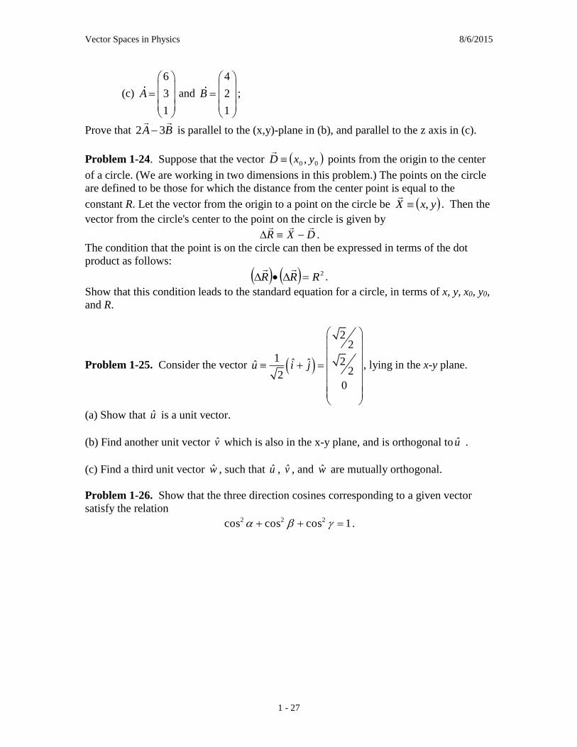
Problem 1-24. Suppose that the vector 00 , yxD
points from the origin to the center
of a circle. (We are working in two dimensions in this problem.) The points on the circle
are defined to be those for which the distance from the center point is equal to the
constant R. Let the vector from the origin to a point on the circle be yxX ,
. Then the
vector from the circle's center to the point on the circle is given by
DXR
.
The condition that the point is on the circle can then be expressed in terms of the dot
product as follows:
2RRR
.
Show that this condition leads to the standard equation for a circle, in terms of x, y, x0, y0,
and R.
Problem 1-25. Consider the vector
22
1 2ˆ ˆˆ22
0
u i j
, lying in the x-y plane.
(a) Show that u is a unit vector.
(b) Find another unit vector v which is also in the x-y plane, and is orthogonal to u .
(c) Find a third unit vector w , such that u , v , and w are mutually orthogonal.
Problem 1-26. Show that the three direction cosines corresponding to a given vector
satisfy the relation
1coscoscos 222 .

Vector Spaces in Physics 8/6/2015
1 - 28
Problem 1-27. Use the dot product and coordinate notation to find the cosine of the
angle between the body diagonal A of the cube
shown and one side B of the cube.
Problem 1-28. Consider the following situation,
analogous to the expansion of the Universe. A swarm
of particles expands through all space, with the
velocity ( )v t of a given particle with position vector
( )r t relative to a fixed origin O given by
( ) ( )dr
v t f t rdt
,
with f(t) some universal function of time. This is the Hubble law.
Show that the same rule applies to positions ( )r t and velocities ( )v t measured relative
to any given particle, say particle A, with position ( )Ar t . That is, show that for
( ) Ar t r t r t and dr
vdt
,
( )v f t r .
This invariance with respect to position in the Universe is sometimes called the
cosmological principle. Can you explain why it implies that we are not at the "center of
the Universe?"
Problem 1-29. It is sometimes convenient to think of a vector B
as having components
parallel to and perpendicular to another vector A
; call these components B and B ,
respectively
(a) Show that
2| |A
ABAB
is parallel to A
and has magnitude equal to the component ˆB A of B
in the direction of
A
; that is, show that
||ˆ ˆB A B A
where as usual A is a unit vector in the direction of A
(and A is its magnitude).
(b) Consider an expression for the part of B
perpendicular to A
:
2A
ABABB
.
Show that
1. B B B
2. 0B A
A
B
a
z
a
y
a
Vector Spaces in Physics 8/6/2015
1 - 29
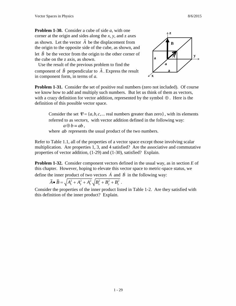
Problem 1-30. Consider a cube of side a, with one
corner at the origin and sides along the x, y, and z axes
as shown. Let the vector A
be the displacement from
the origin to the opposite side of the cube, as shown, and
let B
be the vector from the origin to the other corner of
the cube on the z axis, as shown.
Use the result of the previous problem to find the
component of B
perpendicular to A
. Express the result
in component form, in terms of a.
Problem 1-31. Consider the set of positive real numbers (zero not included). Of course
we know how to add and multiply such numbers. But let us think of them as vectors,
with a crazy definition for vector addition, represented by the symbol . Here is the
definition of this possible vector space.
Consider the set { , , ,... real numbers greater than zero}a b cV , with its elements
referred to as vectors, with vector addition defined in the following way:
a b ab ,
where ab represents the usual product of the two numbers.
Refer to Table 1.1, all of the properties of a vector space except those involving scalar
multiplication. Are properties 1, 3, and 4 satisfied? Are the associative and commutative
properties of vector addition, (1-29) and (1-30), satisfied? Explain.
Problem 1-32. Consider component vectors defined in the usual way, as in section E of
this chapter. However, hoping to elevate this vector space to metric-space status, we
define the inner product of two vectors A and B in the following way:
2 2 2 2 2 2
x y z x y zA B A A A B B B .
Consider the properties of the inner product listed in Table 1-2. Are they satisfied with
this definition of the inner product? Explain.
A
B
a y
x
a
z
a

Vector Spaces in Physics 8/6/2015
2 - 1
Chapter 2. The Special Symbols ij and
ijk , the Einstein
Summation Convention, and some Group Theory
Working with vector components and other numbered objects can be made easier (and
more fun) through the use of some special symbols and techniques. We will discuss two
symbols with indices, the Kronecker delta symbol and the Levi-Civita totally
antisymmetric tensor. We will also introduce the use of the Einstein summation
convention.
References. Scalars, vectors, the Kronecker delta and the Levi-Civita symbol and the
Einstein summation convention are discussed by Lea [2004], pp. 5-17. Or, search the
web. One nice discussion of the Einstein convention can be found at
http://www2.ph.ed.ac.uk/~mevans/mp2h/VTF/lecture05.pdf . You may find other of the
lectures at this site helpful, too.
A. The Kronecker delta symbol, ij .
This symbol has two indices, and is defined as follows:
symbol deltaKronecker 3,2,1,,,1
,0
ji
ji
jiij (2-1)
Here the indices i and j take on the values 1, 2, and 3, appropriate to a space of three-
component vectors. A similar definition could in fact be used in a space of any
dimensionality.
We will now introduce new notation for vector components, numbering them rather
than naming them. [This emphasizes the equivalence of the three dimensions.] We will
write vector components as
, 1,3
x
y i
z
A
A A i
A
(2-2)
We also write the unit vectors along the three axes as
ˆˆ ˆ ˆ, , , 1,3ii j k e i (2-3)
The definition of vector components in terms of the unit direction vectors is
3,1,ˆ ieAA ii
(2-4)
The condition that the unit vectors be orthonormal is
ijji ee ˆˆ (2-5)
This one equation is equivalent to nine separate equations: 1ˆˆ ii , 1ˆˆ jj , 1ˆˆ kk ,
0ˆˆ ji , 0ˆˆ ij , 0ˆˆ ki , 0ˆˆ ik , 0ˆˆ kj , 0ˆˆ jk !!! [We have now stopped
writing "i,j=1,3;" it will be understood from now on that, in a 3-dimensional space, the
"free indices" (like i and j above) can take on any value from 1 to 3.]

Vector Spaces in Physics 8/6/2015
2 - 2
Example: Find the value of kj ˆˆ obtained by using equation (2-5).
Solution: We substitute 2e for j and 3e for k , giving
0ˆˆˆˆ2332 eekj ,
correct since j and k are orthogonal.
B. The Einstein summation convention.
The dot product of two vectors A
and B
now takes on the form
3
1i
ii BABA
. (2-6)
This is the same dot product as previously defined in equation (1-40), except that AxBx
has been replaced by A1B1 and so on for the other components.
Now, when you do a lot of calculations with vector components, you find that the sum of
an index from 1 to 3 occurs over and over again. In fact, occasions where the sum would
not be carried out over all three of the directions are hard to imagine. Furthermore, when
a sum is carried out, there are almost always two indices which have the same value - the
index i in equation (2-6) above, for example. So, the following practice makes the
equations much simpler:
This sounds a bit risky, doesn't it? Will you always know when to sum and when not to?
It does simplify things, though. The reference to tensor indices means indices on
elements of matrices. We will see that this convention is especially well adapted to
matrix multiplication.
So, the definition of the dot product is now
ii BABA
, (2-7)
the same as equation (2-6) except that the summation sign is omitted. The sum is still
carried out because the index i appears twice, and we have adopted the Einstein
summation convention.
To see how this looks in practice, let's look at the calculation of the x-component of a
vector, in our new notation. We will write the vector A
, referring to the diagram of
figure 1-11, as
The Einstein Summation Convention. In expressions involving vector or tensor indices,
whenever two indices are the same (the same symbol), it will be assumed that a sum over
that index from 1 to 3 is to be carried out. This index is referred to as a paired index;
paired indices are summed. An index which only occurs once in a term of an expression is
referred to as a free index, and is not summed.

Vector Spaces in Physics 8/6/2015
2 - 3
ii
zyx
Ae
AkAjAiA
ˆ
ˆˆˆ
, (2-8)
where in the second line the summation over i = {1,2,3} is implicit. Now use the
definition of the x-component,
11 eAAAx
. (2-9)
Combining (2-8) and (2-9), we have
1 1
1
1
1
1
ˆ
ˆ ˆ( )
ˆ ˆ( )
i i
i i
i i
A A e
e A e
A e e
A
A
(2-10)
In the next to last step we used (2-5), the orthogonality condition for the unit direction
vectors.
Next we carried out one of the most important operations using the Kronecker delta
symbol, summing over one of its indices. This is also very confusing to someone seeing
it for the first time. In the last line of equation (2-10) there is an implied summation over
the index i. We will write out that summation term by term, just this once:
3132121111 AAAA ii (2-11)
Now refer to (2-1), the definition of the Kronecker delta symbol. What are the values of
the three delta symbols on the right-hand side of the equation above? Answer: 11 = 1,
21 = 0, 31 = 0. Substituting these values in gives
1
321
3132121111
001
A
AAA
AAAA ii
(2-12)
What has happened? The index "1" has been transferred from the delta symbol to A.
C. The Levi-Civita totally antisymmetric tensor.
The Levi-Civita symbol is an object with three vector indices,
, 1, 2,3; 1,2,3; 1,2,3 Levi-Civita Symbol
1, , , an even permutation of 1,2,3
1, , , an odd permutation of 1,2,3
0 otherwise
ijk
ijk
i j k
i j k
i j k
(2-13)
All of its components (all 27 of them) are either equal to 0, -1, or +1. Determining which
is which involves the idea of permutations. The subscripts (i,j,k) represent three
numbers, each of which can be equal to 1, 2, or 3. A permutation of these numbers
scrambles them up, and it is a good idea to approach this process systematically. So, we
are going to discuss the permutation group.

Vector Spaces in Physics 8/6/2015
2 - 4
Groups. A group is a mathematical concept, a special kind of set. It is defined as
follows:
Definition: A group G is a set of objects , , ,...A B C with multiplication of one
member by another defined, closed under multiplication, and with the additional
properties:
(i) The group contains an element I called the identity, such that, for every
element A of the group,
AI IA A (2-14)
(ii) For every element A of the group there is another element B, such that
AB BA I . (2-15)
B is said to be the inverse of A:
1A B . (2-16)
(iii) Multiplication must be associative:
A BC AB C . (2-17)
There is an additional property which only some groups have. If multiplication is
independent of the order in the product, the group is said to be Abelian.
Otherwise, the group is non-Abelian.
Abelian groupAB BA . (2-18)
This may seem fairly abstract. But the members of groups used in physics are usually
operators, operating on interesting things, such as vectors or members of some other
vector space. Right now we are going to consider permutation operators, operating on
sets of indices.
The Permutation Group. We will start by defining the objects operated on, then the
operators themselves. Consider the numbers 1, 2, and 3, in some order, just like the
indices on the Levi-Civita symbol:
( , , )a b c . (2-19)
Here each letter represents one of the numbers, and they all three have to be represented.
It is pretty easy to convince yourself that the full set of possibilities is
( , , ) 1,2,3 , 1,3,2 , 2,1,3 , 2,3,1 , 3,1,2 , 3,2,1a b c . (2-20)
Now the permutation group of the third degree consists of operators which re-arrange the
three numbers as follows:
123
132
213
231
312
321
, , , ,
, , , ,
, , , ,
, , , ,
, , , ,
, , , ,
P a b c a b c P I
P a b c a c b P
P a b c b a c P
P a b c b c a P
P a b c c a b P
P a b c c b a P
. (2-21)
Vector Spaces in Physics 8/6/2015
2 - 5
The second form of the notation shows where the numbers (1,2,3) would end up under
that permutation. The first entry is the permutation which doesn't change the order,
which is evidently the identity for the group. The group consists of just these six
members
Examples of permutations operating on triplets of indices:
123
132
321
132 321
2,3,1 2,3,1
2,3,1 2,1,3
2,3,1 1,3, 2
2,3,1 1,2,3
P
P
P
P P
. (2-22)
Do you follow the fourth line? First the permutation P321 is carried out, giving (1,3,2);
and then the permutation P132 operates on this result, giving (1,2,3). This brings us to the
subject of multiplication of group elements. This fourth line shows us that the product of
the given two permutation-group elements is itself a permutation, namely
132 321 312P P P . (2-23)
Try this yourself, and verify that
312 2,3,1 1,2,3P . (2-24)
From this example, it is pretty clear that the group of six elements given above is closed
under multiplication. There is an identity, the permutation which doesn't change the
order. And it is pretty easy to identify the inverses within the group.
Example: Show that
1
312 231P P .
Proof: Try it out on the triplet (a,b,c):
312
231
, , , ,
, , , ,
p a b c c a b
P c a b a b c
.
The inverse permutation P231 just reverses the effect of P312.
There are some simpler permutation operators related to the Pijk, the binary permutation
operators which just interchange a pair of indices, while leaving the third one unchanged.
12
13
23
, , , ,
, , , ,
, , , ,
P a b c b a c
P a b c c b a
P a b c a c b
. (2-25)
It is easy to see that the six group members given in equation (2-21) can be written in
terms of the binary permutation operators:

Vector Spaces in Physics 8/6/2015
2 - 6
2 2 2
123 12 13 23
132 23
213 12
231 12 13
312 13 12
321 13
P I P P P
P P
P P
P P P
P P P
P P
. (2-26)
(Remember, the right-hand operator in a product operates first.)
There is a special subset of permutations of a series of objects called the circular
permutations, where the last index comes to the front and the others all move over one
(see Figure 2-1).
For the six objects listed in eq. (2-21), three of them are circular permutations of (1,2,3),
namely
circular( , , ) 1,2,3 , 3,1,2 , 2,3,1a b c . (2-27)
Each of these is produced by an even number of binary permutations, and the other three
are produced by an odd number of binary permutations. So, the group divides up into
three "even permutations" and three "odd permutations:"
123
312
231
213
132
321
even permutations
odd permutations
P
P
P
P
P
P
. (2-28)
The Levi-Civita symbol. Now we can finally use the idea of even and odd permutations
to define the Levi-Civita symbol:
Symbol Civita-Levi
otherwise 0
(123) ofn permutatio oddan (ijk) 1,-
(123) ofn permutatioeven an (ijk) 1,
ijk (2-29)
Notice that there are only six non-zero symbols, three equal to +1 and three equal to -1.
And any binary permutation of the indices (interchanging two indices) changes the sign.
This is the key property in many calculations using the Levi-Civita symbol.
Example: Give the values of 312, 213, and 322,
(a,b,c,d,e,f,g) ---> (g,a,b,c,d,e,f)
Figure 2-1. A circular permutation.
Vector Spaces in Physics 8/6/2015
2 - 7
Answer: (312) is an even permutation of (123), so 312 = +1. (213) is obtained
from (312) by permuting the first and last numbers, so it must be an odd
permutation, and 213 = -1. (322) is not a permutation of (123) at all, so 322 = 0.
Question: Is the permutation group Abelian? What about the subgroup consisting of the
three circular permutations? Answering these questions will be left to the problems.
D. The cross product.
In the last chapter we found the following result for the cross product of two vectors A
and B
in terms of their components:
)(ˆ
)(ˆ
)(ˆ
xyyx
zxxz
yzzy
BABAk
BABAj
BABAiBA
(1-48)
Notice that there are a lot of permutations built into this definition. In particular, each
term involves a permutation of (x,y,z), with the first letter indicating the unit vector, the
second, the component of A, and the third, the component of B. Here is an elegant way of
re-writing this expression using the Levi-Civita symbol:
kjijki BABA
(2-30)
It may be less than obvious at first glance that (2-30) is the equivalent of (1-48). First
let's just examine the index structure of the expression. The left-hand side has a single
unpaired, or free, index, i. This means that it represents any single one of the components
of the vector BA
- we would say that it gives the i-th component of BA
. Now look
at the right-hand side. There is only one free index, and it is i, the same as on the left-
hand side. This is the way it has to be. In addition, there are two paired indices, j and k.
These have to be summed. If we were not using the Einstein summation convention, this
expression would read kjijk
kj
i BABA
3
1
3
1
. We have decided to follow the
Einstein convention and so we will not write the summation signs. However, for any
given value of i, there are nine terms to evaluate.
To see exactly how this works out, let's evaluate the result of (2-30) for i=2. This
should give the y-component of BA
. Here it is:
332332323213231
322232222212221
312132121211211
22
BABABA
BABABA
BABABA
BABA kjjk
(2-31)
But, most of these terms are equal to zero, because two of the indices on the Levi-Civita
symbol are the same. There are only two non-zero L.-C. symbols: 213 = -1, and 231 =
+1. Using these facts, we arrive at the answer
Vector Spaces in Physics 8/6/2015
2 - 8
13312 BABABA
(2-32)
This is the same as the y-component of equation (1-48), if the correct substitutions are
made for numbered instead of lettered components. So, the two versions of the cross
product agree.
Example: Use the tensor form of the cross product, equation (2-30), to prove that
ABBA
.
Proof: There was a similar relation for the dot product - but with a plus sign!
Let's see how this works in tensor notation:
product cross theof definition
orderany in written becan B theand A the
sign minus a gives ε of indices twopermuting
product cross theof definition
kj
i
jkikj
kjikj
kjijki
AB
AB
BA
BABA
In regard to the last step of this example, it is worth remarking that particular name
given to a summed index doesn't matter - it is sort of like the dummy variable inside a
definite integral. What matters in the definition of the cross product BA
is that the
index of the components of A match with the second index of , and the index of the
components of B, with the third index of .
E. The triple scalar
product.
There is a famous way of
making a scalar out of three
vectors. It is illustrated in
figure 2-2, where the vectors
A
, B
and C
form the three
independent sides of a
parallelopiped. The cross
product of B
and C
gives
the area of the base of the
parallelopiped (a
parallelogram), and dotting
with A
gives the volume:
CBA
Volume . (2-31)
Putting in the forms of the dot and cross product using , we have
area of parallelogram =
magnitude of BxC.
height ofrectangular
solid
B
C
A BxC
Figure 2-2. A parallelepiped, with its sides defined by
vectors A, B and C. The area of the parallelogram forming
the base of this solid is equal to BC sin , where is the
angle between B and C. This is just the magnitude of the
cross product BxC. When BxC is dotted into A, the area of
the base is multiplied by the height of the solid, giving its
volume.

Vector Spaces in Physics 8/6/2015
2 - 9
kjiijk
kjijki
ii
CBA
CBA
CBA
CBA
CBA
Volume
. (2-33)
There is an identity involving the triple scalar product which is easy to demonstrate from
this form:
BACACBCBA
. (2-34)
In the geometrical interpretation of the triple scalar product, these three forms correspond
to the three possible choices of which side of the parallelepiped to call the base (see
figure 2-2).
F. The triple vector product.
There is another way to combine three vectors, this time giving another vector:
CBAD
(triple vector product) (2-35)
In tensor notation this becomes
mlklmjijk
kjijk
ii
CBA
CBA
CBAD
(2-36)
This is not very encouraging. It is not simple, and furthermore it conjures up the prospect
of more cross products. Do we have to live in dread of CBAD
and all of her big
sisters?
The Epsilon Killer. Happily there is a solution. There is an identity which guarantees
that there will never be more than one ijk in an expression, by reducing a product of two
epsilons to Kronecker deltas. Here it is:
kljmkmjlilmijk (2-37)
This is the epsilon killer! Here are the important structural features. There are two
epsilons, with the first index of each one the same, so there is a sum over that index. The
other four indices (two from each epsilon) are all different, and so are not summed. We
will not prove eq. (2-37), but it is not too difficult, if you just consider all the possibilities
for the indices.
We will now use this identity to simplify the expression for the vector triple product:
deltas of indices pairedover sum
killerepsilon use )(
indices ofn permutatio cyclic
product cross of definition
illmim
mljjlimjmil
mljklmkij
mlklmjijki
CBACBA
CBA
CBA
CBACBA
(2-38)
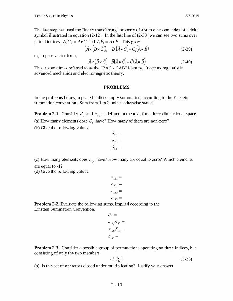
Vector Spaces in Physics 8/6/2015
2 - 10
The last step has used the "index transferring" property of a sum over one index of a delta
symbol illustrated in equation (2-12). In the last line of (2-38) we can see two sums over
paired indices, CACA mm
and .BABA ll
This gives
BACCABCBA iii
(2-39)
or, in pure vector form,
BACCABCBA
(2-40)
This is sometimes referred to as the "BAC - CAB" identity. It occurs regularly in
advanced mechanics and electromagnetic theory.
PROBLEMS
In the problems below, repeated indices imply summation, according to the Einstein
summation convention. Sum from 1 to 3 unless otherwise stated.
Problem 2-1. Consider ij and ijk as defined in the text, for a three-dimensional space.
(a) How many elements does ij have? How many of them are non-zero?
(b) Give the following values:
31
23
11
(c) How many elements does ijk have? How many are equal to zero? Which elements
are equal to -1?
(d) Give the following values:
132
123
321
111
Problem 2-2. Evaluate the following sums, implied according to the
Einstein Summation Convention.
jj
kk
jj
ii
1
112
312
Problem 2-3. Consider a possible group of permutations operating on three indices, but
consisting of only the two members
12,I P (3-25)
(a) Is this set of operators closed under multiplication? Justify your answer.

Vector Spaces in Physics 8/6/2015
2 - 11
(b) Is this set of operators Abelian? Justify your answer.
Problem 2.4. Consider a possible group of permutations operating on three indices, but
consisting of only the four members
12 13 23, , ,I P P P (3-25)
(a) Is this set of operators closed under multiplication? Explain your answer.
(b) Is this set of operators Abelian? Explain your answer.
Problem 2.5. Consider the full permutation group, operating on three indices.
(a) Is the group Abelian? Explain your answer.
(b) What about the subgroup consisting of just the two circular permutations (and the
identity)? Explain your answer.
[You might approach these questions by simply trying two successive permutations, and
then reversing the order.]
Problem 2-6. Assume that the cross product D A B is defined by the relation
i ijk j ki
D A B A B .
Show using tensor notation (rather than writing out all the terms) that the magnitude of
this vector agrees with the geometrical definition of the cross product. That is, show that
D has a magnitude equal to |ABsin|. [Hint: Evaluate D D using the ''epsilon-killer''
identity.]
Problem 2-7. Use tensor notation (rather than writing out all the terms) to prove the
following identity for three arbitrary vectors A
, B
, and C
.
BACACBCBA
Problem 2-8. (a) Use tensor notation (rather than writing out all the terms) to prove the
following identity for two arbitrary vectors A
and B
.
0 BAA
[Hint: Use the symmetries of the Levi-Civita symbol to prove that
BAABAA
. This
implies that both sides of the equation are equal to zero.]
(b) Make a geometrical argument, based on the direction of A B , to show that this
identity has to be satisfied.
Problem 2-9. Let 3,2,1,ˆ iei be the usual three directional unit vectors of a 3-
dimensional Cartesian coordinate system, satisfying the orthonormality relation
ijji ee ˆˆ . In terms of components, A
and B
can be written as

Vector Spaces in Physics 8/6/2015
2 - 12
ˆ ,
ˆ .
m m
j j
A A e
B B e
Using these definitions for A and B and using tensor notation, show that
ii BABA
.

Vector Spaces in Physics 8/6/2015
3 - 1
Chapter 3. Linear Equations and Matrices
A wide variety of physical problems involve solving systems of simultaneous linear
equations. These systems of linear equations can be economically described and
efficiently solved through the use of matrices.
A. Linear independence of vectors.
Let us consider the three vectors 1E , 2E and 3E given below.
1 1
2 2
3 3
2
1 , 1,3
1
4
3 , 1,3
3
3
2 , 1,3
1
i
i
i
E E i
E E i
E E i
(3-1)
These three vectors are said to be linearly dependent if there exist constants c1, c2, and c3,
not all zero, such that
1 1 2 2 3 3 0ij jc E c E c E E c (3-2)
The second form in the equation above gives the i-th component of the vector sum as an
implied sum over j, invoking the Einstein summation convention. Substituting in the
values for the components ijE from equation (3.1), this vector equation is equivalent to
the three linear equations:
03
023
0342
321
321
321
ccc
ccc
ccc
(3-3)
These relations are a special case of a more general mathematical expression,
dcA
(3-4)
where c
and d
are vectors represented as column matrices, and A is a sort of operator
which we will represent by a square matrix.
The goal of the next three chapters is to solve equation (3-4) by the audacious leap of
faith,

Vector Spaces in Physics 8/6/2015
3 - 2
dAc 1 (3-5)
.What is 1A ? Dividing by a matrix!?! We will come to this later.
B. Definition of a matrix.
A matrix is a rectangular array of numbers. Below is an example of a matrix of
dimension 3x4 (3 rows and 4 columns).
4,1,3,1,
1121
1221
1112
jiAA ij (3-6)
We will follow the "RC convention" for numbering elements of a matrix, where Aij is the
element of matrix A in its i-th row
and j-th column. As an example, in
the matrix above, the elements which
are equal to -1 are A13, A21, and A34.
C. The transpose of a matrix.
The transpose TA of a matrix A is
obtained by drawing a line down the
diagonal of the matrix and moving
each component of the matrix across
the diagonal to the position where its
image would be if there were a mirror
along the diagonal of the matrix:
This corresponds to the interchange
of the indices on all the components
of A :
ji
T
ij AA Transpose (3-7)
Example: Calculate the transpose of the square matrix given below:
131
231
342
A (3-8)
Solution:
123
334
112
131
231
342transpose
(3-9)
mirror line
Figure 3-1. The transpose operation moves
elements of a matrix from one side of the
diagonal to the other.
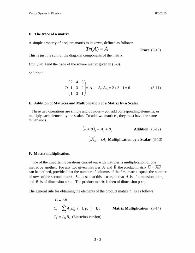
Vector Spaces in Physics 8/6/2015
3 - 3
D. The trace of a matrix.
A simple property of a square matrix is its trace, defined as follows:
iiAATr )( Trace (3-10)
This is just the sum of the diagonal components of the matrix.
Example: Find the trace of the square matrix given in (3-8).
Solution:
6132
131
231
342
332211
AAATr (3-11)
E. Addition of Matrices and Multiplication of a Matrix by a Scalar.
These two operations are simple and obvious – you add corresponding elements, or
multiply each element by the scalar. To add two matrices, they must have the same
dimensions.
ijijij BABA Addition (3-12)
ijij cAAc Multiplication by a Scalar (3-13)
F. Matrix multiplication.
One of the important operations carried out with matrices is multiplication of one
matrix by another. For any two given matrices A and B the product matrix BAC
can be defined, provided that the number of columns of the first matrix equals the number
of rows of the second matrix. Suppose that this is true, so that A is of dimension p x n,
and B is of dimension n x q. The product matrix is then of dimension p x q.
The general rule for obtaining the elements of the product matrix C is as follows:
1
, 1, , 1,
(Einstein's version)
n
ij ik kj
k
ij ik kj
C AB
C A B i p j q
C A B
Matrix Multiplication (3-14)

Vector Spaces in Physics 8/6/2015
3 - 4
This illustrated below, for A a 3 x 4 matrix and B
a 4 x 2 matrix.
1 32 1 1 1 3
2 21 2 2 1 8
2 11 2 1 1 0
1 1
AB C
x
y
z
(3-15)
Example: Calculate the three missing elements x. y, and z in the result matrix
above.
Solution:
5
1*)1()1(*12*23*1
6
)1(*12*2)2(*)2(1*)1(
;10
1*1)1(*)1(2*13*2
21
4
1
21
12
z
Cy
BA
Cx
k
kn
There is a tactile way of remembering how to do this multiplication, provided that the
two matrices to be multiplied are written down next to each other as in equation (3-15).
Place a finger of your left hand on Ai1, and a finger of your right hand on B1j. Multiply
together the two values under your two fingers. Then step across the matrix A from left
to right with the finger of your left hand, simultaneously stepping down the matrix B
with the finger of your right hand. As you move to each new pair of numbers, multiply
them and add to the previous sum. When you finish, you have the value of Cij. For
instance, calculating C21 in the example of equation (3-15) this way gives -1 + 4 + 4 - 1 =
6.
Einstein Summation Convention. For the case of 3x3 matrices operating on 3-
component column vectors, we can use the Einstein summation convention to write
matrix operations:
matrix multiplying vector:
jiji xAy
xAy
(3-16)
matrix multiplying matrix:

Vector Spaces in Physics 8/6/2015
3 - 5
kjikij BAC
BAC
(3-17)
The rules for matrix multiplication may seem complicated and arbitrary. You might
ask, "Where did that come from?" Here is part of the answer. Look at the three
simultaneous linear equations given in (3-3) above. They are precisely given by
multiplying a matrix A of numerical coefficients into a column vector c
of variables, to
wit:
0
0
0
131
231
342
;0
3
2
1
c
c
c
cA
(3-18)
The square matrix above is formed of the components of the three vectors 1E
, 2E
and 3E
, placed as its columns:
321 EEEA
(3-18a)
This matrix representation of a system of linear equations is very useful.
Exercise: Use the rules of matrix multiplication above to verify that (3-18) is
equivalent to (3-3).
G. Properties of matrix multiplication.
Matrix multiplication is not commutative. Unlike multiplication of scalars, matrix
multiplication depends on the order of the matrices:
ABBA (3-19)
Matrix multiplication is thus said to be non-commutative.
Example: To investigate the non-commutativity of matrix multiplication, consider
the two 2x2 matrices A and B :
21
12
,34
21
B
A
(3-20)
Calculate the two products BA and AB and compare.

Vector Spaces in Physics 8/6/2015
3 - 6
Solution:
1011
54
21
12
34
21BA (3-21)
but
47
12
34
21
21
12AB (3-22)
The results are completely different.
Other properties. The following properties of matrix multiplication are easy to verify.
CBACBA Associative Property (3-23)
CABACBA Distributive Property (3-24)
H. The unit matrix.
A useful matrix is the unit matrix, or the identity matrix,
ijI
100
010
001
(3-25)
This matrix has the property that, for any square matrix A ,
AIAAI (3-26)
I has the same property for matrices that the number 1 has for scalar multiplication.
This is why it is called the unit matrix.
I. Square matrices as members of a group. The rules for matrix multiplication given
above apply to matrices of arbitrary dimension. However, square matrices (number of
rows equals the number of columns) and vectors (matrices consisting of one column)
have a special interest in physics, and we will emphasize this special case from now on.
The reason is as follows: When a square matrix multiplies a column matrix, the result is
another column matrix. We think of this as the matrix "operating" on a vector to produce
another vector. Sets of operators like this, which transform one vector in a space into
another, can form groups. (See the discussion of groups in Chapter 2.) The key
characteristic of a group is that multiplication of one member by another must be defined,
in such a way that the group is closed under multiplication; this is the case for square
matrices. (An additional requirement is the existence of an inverse for each member of
the group; we will discuss inverses soon.)

Vector Spaces in Physics 8/6/2015
3 - 7
Notice that rotations of the coordinate system form a group of operations: a rotation of
a vector produces another vector, and we will see that rotations of 3-component vectors
can be represented by 3x3 square matrices. This is a very important group in physics.
J. The determinant of a square matrix.
For square matrices a useful scalar quantity called the determinant can be calculated.
The definition of the determinant is rather messy. For a 2 x 2 matrix, it can be defined as
follows:
bcaddc
ba
dc
ba
det (3-27)
That is, the determinant of a 2 x 2 matrix is the product of the two diagonal elements
minus the product of the other two. This can be extended to a 3x3 matrix as follows:
)()()( gedhcgfdibhfeia
hg
edc
ig
fdb
ih
fea
ihg
fed
cba
(3-28)
Example: Calculate the determinant of the square matrix A of eq. (3-18) above.
Result:
2
)33(3)21(4)63(2
131
231
342
(3-29)

Vector Spaces in Physics 8/6/2015
3 - 8
The form (3-28) for the determinant can be put in a more general form if we make a few
definitions. If A is a square nxn matrix, its (i,j)-th minor Mij is defined as the
determinant of the (n-1)x(n-1) matrix formed by removing the i-th row and j-th column of
the original matrix. In (3-28) we see that a is multiplied by its minor, -b is multiplied by
the minor of b, and c is multiplied by its minor. We can then write, for a 3 x 3 matrix A ,
3
1
1
1
1 1j
j
j
j MAA (3-30)
[Notice that j occurs three times in this expression, and we have been obliged to back
away from the Einstein summation convention and write out the sum explicitly.] This
expression could be generalized in the obvious way to a matrix of an arbitrary number of
dimensions n, merely by summing from j = 1 to n .
The 3 x 3 determinant expressed with the Levi-Civita tensor.
Loving the Einstein summation convention as we do, we are piqued by having to give it
up in the preceding definition of the determinant. For 3x3 matrices we can offer the
following more elegant definition of the determinant. If we write out the determinant of a
3 x 3 matrix in terms of its components, we get
312213322113
312312332112322311332211
AAAAAA
AAAAAAAAAAAAA
(3-31)
Each term is of the form A1iA2jA3k, and it is not too hard to see that the terms where (ijk)
are an even permutation of (123) have a positive sign, and the odd permutations have a
negative sign. That is,
m={{2,4,3},{1,3,2},{1,3,1}} defining a matrix
MatrixForm[m] display as a rectangular array
cm multiply by a scalar
a . b matrix product
Inverse[m] matrix inverse
MatrixPower[m,n] nth power of a matrix
Det[m] determinant
Tr[m] trace
Transpose[m] transpose
Eigenvalues[m] eigenvalues
Engenvectors[m] eigenvectors
Eigenvalues[N[m]],Eigenvectors[N[m]] numerical eigenvalues and eigenvectors
m=Table[Random[],{3},{3}] 3x3 matrix of random numbers
Table 3-1. Some mathematical operations on matrices which Mathematica can carry
out.
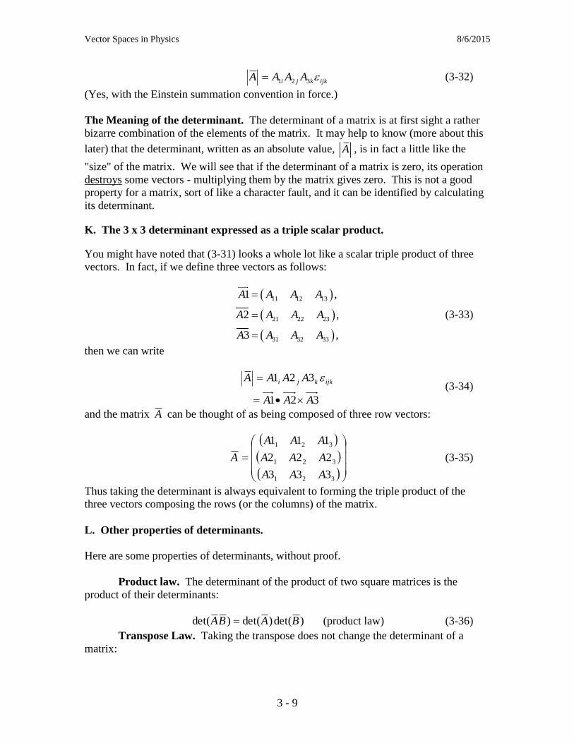
Vector Spaces in Physics 8/6/2015
3 - 9
ijkkji AAAA 321 (3-32)
(Yes, with the Einstein summation convention in force.)
The Meaning of the determinant. The determinant of a matrix is at first sight a rather
bizarre combination of the elements of the matrix. It may help to know (more about this
later) that the determinant, written as an absolute value, A , is in fact a little like the
"size" of the matrix. We will see that if the determinant of a matrix is zero, its operation
destroys some vectors - multiplying them by the matrix gives zero. This is not a good
property for a matrix, sort of like a character fault, and it can be identified by calculating
its determinant.
K. The 3 x 3 determinant expressed as a triple scalar product.
You might have noted that (3-31) looks a whole lot like a scalar triple product of three
vectors. In fact, if we define three vectors as follows:
11 12 13
21 22 23
31 32 33
1 ,
2 ,
3 ,
A A A A
A A A A
A A A A
(3-33)
then we can write
321
321
AAA
AAAA ijkkji
(3-34)
and the matrix A can be thought of as being composed of three row vectors:
321
321
321
333
222
111
AAA
AAA
AAA
A (3-35)
Thus taking the determinant is always equivalent to forming the triple product of the
three vectors composing the rows (or the columns) of the matrix.
L. Other properties of determinants.
Here are some properties of determinants, without proof.
Product law. The determinant of the product of two square matrices is the
product of their determinants:
)det()det()det( BABA (product law) (3-36)
Transpose Law. Taking the transpose does not change the determinant of a
matrix:
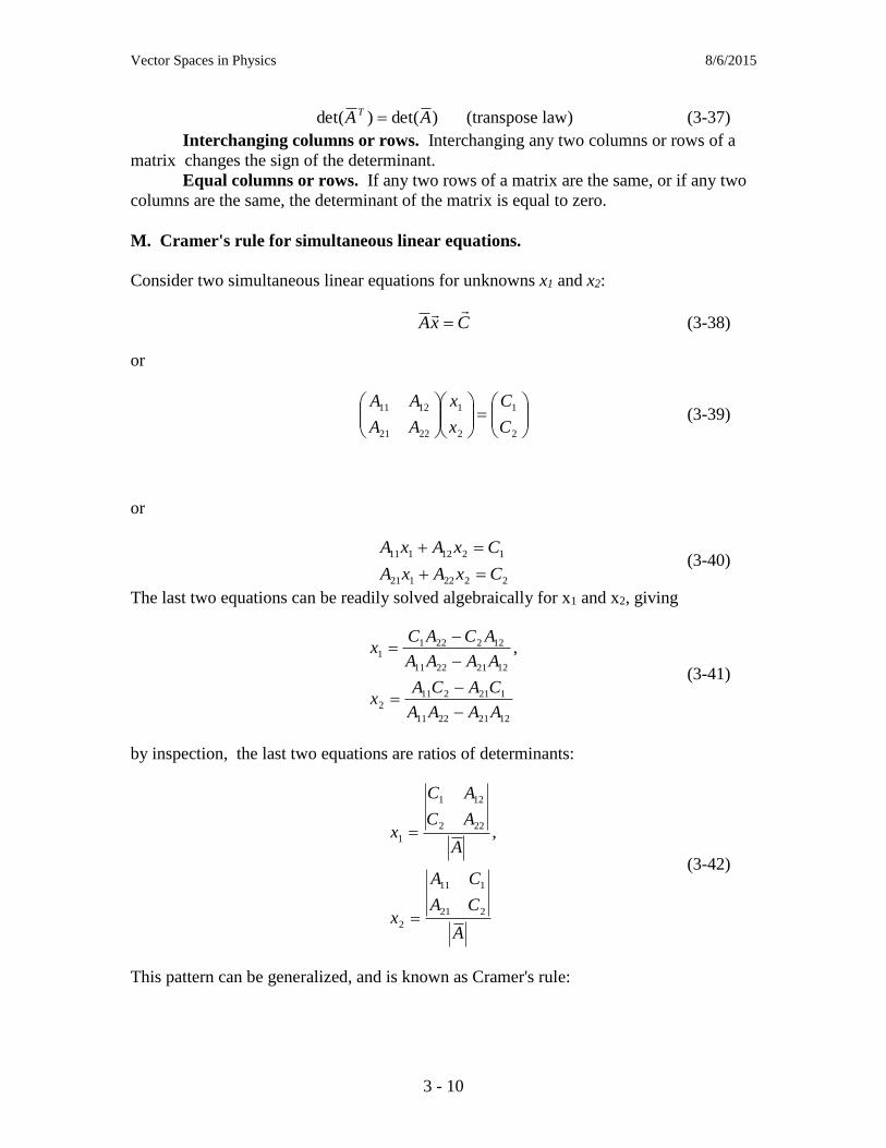
Vector Spaces in Physics 8/6/2015
3 - 10
)det()det( AAT (transpose law) (3-37)
Interchanging columns or rows. Interchanging any two columns or rows of a
matrix changes the sign of the determinant.
Equal columns or rows. If any two rows of a matrix are the same, or if any two
columns are the same, the determinant of the matrix is equal to zero.
M. Cramer's rule for simultaneous linear equations.
Consider two simultaneous linear equations for unknowns x1 and x2:
CxA
(3-38)
or
2
1
2
1
2221
1211
C
C
x
x
AA
AA (3-39)
or
2222121
1212111
CxAxA
CxAxA
(3-40)
The last two equations can be readily solved algebraically for x1 and x2, giving
12212211
1212112
12212211
1222211 ,
AAAA
CACAx
AAAA
ACACx
(3-41)
by inspection, the last two equations are ratios of determinants:
A
CA
CA
x
A
AC
AC
x
221
111
2
222
121
1 ,
(3-42)
This pattern can be generalized, and is known as Cramer's rule:

Vector Spaces in Physics 8/6/2015
3 - 11
A
AACAAA
C
C
AACAAA
AACAAA
xnninninnn
n
nii
nii
i
....
.........
..........
..........
..........
..........
..........
.........
....
....
1,1,21
1
3
21,22.1,22221
11,111,11211
(3-43)
As an example of using Cramer's rule, let us consider the three simultaneous linear
equations for x1, x2, and x3 which can be written
4
1
1
131
231
342
;
3
2
1
x
x
x
CxA
(3-44)
First we calculate the determinant A :
2
)0(3)1(4)3(231
313
11
214
13
232
131
231
342
A
(3-45)
The values for the xi are then given by
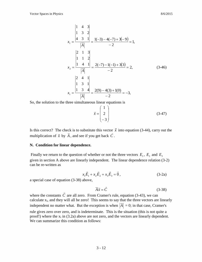
Vector Spaces in Physics 8/6/2015
3 - 12
,32
)0(1)3(4)9(2431
131
142
,22
33)1(1)7(2141
211
312
,12
93)7(4)3(1134
231
341
1
2
1
Ax
Ax
Ax
(3-46)
So, the solution to the three simultaneous linear equations is
3
2
1
x
(3-47)
Is this correct? The check is to substitute this vector x into equation (3-44), carry out the
multiplication of x by A , and see if you get back C .
N. Condition for linear dependence.
Finally we return to the question of whether or not the three vectors 1E , 2E and 3E
given in section A above are linearly independent. The linear dependence relation (3-2)
can be re-written as
0332211
ExExEx , (3-2a)
a special case of equation (3-38) above,
CxA
(3-38)
where the constants C
are all zero. From Cramer's rule, equation (3-43), we can
calculate xi, and they will all be zero! This seems to say that the three vectors are linearly
independent no matter what. But the exception is when A = 0; in that case, Cramer's
rule gives zero over zero, and is indeterminate. This is the situation (this is not quite a
proof!) where the xi in (3.2a) above are not zero, and the vectors are linearly dependent.
We can summarize this condition as follows:

Vector Spaces in Physics 8/6/2015
3 - 13
dependentlinearly are ,,0 321321 EEEEEE
(3-48)
Example: As an illustration, let us take the vectors 1E
and 3E
from eq. (3-1), and
construct a new vector 4E
by taking their sum:
2
3
5
1
2
3
1
1
2
314 EEE
(3-49)
1E
, 3E
and 4E
are clearly linearly dependent, since 1E
+ 3E
-4E
= 0
. We form the
matrix A by using 1E
, 3E
and 4E
for its columns:
211
321
532
431 EEEA
(3-50)
Now the acid test for linear dependence: calculate the determinant of A :
0)1(5)1(3)1(2
211
321
532
A (3-51)
This confirms that 1E
, 3E
and 4E
are linearly dependent.
There is a final observation to be made about the condition (3-48) for linear dependence.
The determinant of a 3x3 matrix can be interpreted as the cross product of the vectors
forming its rows or columns. So, if the determinant is zero, it means that
0321 EEE
, and this has the following geometrical interpretation: If 1E
is
perpendicular to 32 EE
, it must lie in the plane formed by 2E
and 3E
; if this is so, it
is not independent of 2E
and 3E
.
O. Eigenvectors and eigenvalues.
For most matrices A there exist special vectors V which are not changed in direction
under multiplication by A :
AV V (3-52)
In this case V is said to be an eigenvector of A and is the corresponding eigenvalue.
In many physical situations there are special, interesting states of a system which are
invariant under the action of some operator (that is, invariant aside from being multiplied
by a constant, the eigenvalue). Some very important operators represent the time

Vector Spaces in Physics 8/6/2015
3 - 14
evolution of a system. For instance, in quantum mechanics, the Hamiltonian operator
moves a state forward in time, and its eigenstates represent "stationary states," or states of
definite energy. We will soon see examples in mechanics of coupled masses where the
eigenstates describe the normal modes of motion of the system. Eigenvectors are in
general charismatic and useful.
So, what are the eigenstates and eigenvalues of a square matrix? The eigenvalue
equation, (3-52) above, can be written
0A I V (3-53)
or, for the case of a 3x3 matrix,
11 12 13 1
21 22 23 2
31 32 33 3
0
0
0
A A A V
A A A V
A A A V
(3-54)
As discussed in the last section, the condition for the existence of solutions for the
variables 1 2 3, ,V V V is that the determinant
11 12 13
21 22 23
31 32 33
A A A
A A A
A A A
(3-55)
vanish. This determinant will give a cubic polynomial in the variable , with in general
three solutions, ( ) (1) (2) (3), ,i . For each value, the equation
0
i iA I V (3-56)
can be solved for the components of the i-th eigenvector ( )iV .
Example: Rotation about the z axis.
In Chapter 1 we found the components of a vector rotated by an angle about the
z axis. Including the fact that the z component does not change, this rotation can
be represented as a matrix operation,
zx R x (3-57)
where
cos sin 0
sin cos 0
0 0 1
zR
(3-58)
Now, based on the geometrical properties of rotating about the z axis, what vector
will not be changed? A vector in the z direction! So, an eigenvector of zR is
1
0
0
1
V
(3-59)

Vector Spaces in Physics 8/6/2015
3 - 15
Try it out:
1
cos sin 0 0 0
sin cos 0 0 0
0 0 1 1 1
zR V
(3-60)
1V is an eigenvector of zR , with eigenvalue 1
1 .
PROBLEMS
Problem 3-1. Consider the square matrix
121
132
311
B .
(a) Calculate the transpose of B .
(b) Verify by direct calculation that TBB detdet .
Problem 3-2. Consider the two matrices
131
231
342
A
and
121
132
311
B .
If C is the product matrix, BAC , verify by direct calculation that
BABAC detdetdetdet .
Problem 3.2a. There is a useful property of the determinant, stated in Problem 3-2
above, which is rather hard to prove algebraically:
BABAC detdetdetdet ,
where A , B and C are square matrices of the same dimension. Let's consider a
numerical "proof" of this theorem, using Mathematica. (See Table 3-1 for a collection of
useful Mathematica operations.)
(a) Fill two 4x4 matrices - call them A and B - with random numbers.
(b) Calculate their determinants.
(c) Calculate the product matrix BAC , and the determinant of C .
(d) See if the theorem above is satisfied in this case.
Vector Spaces in Physics 8/6/2015
3 - 16
(e) Another theorem concerning square matrices is stated in Problem 3-1 above. Test
it, for both of your random matrices.
Problem 3-3. Using tensor notation and the Einstein summation convention, prove the
following theorem about the transpose of the product of two square matrices: If C is the
product matrix, BAC , then T T TC B A .
[As a starting point, under the Einstein Summation Convention,
ij il ljC A B .]
Problem 3-4. Calculate Idet and ITr , where I is the nxn identity matrix.
Problem 3-5. Starting with the definition (3-30) of the determinant, but generalized to n
dimensions by carrying out the sum over j from 1 to n, use the fact that interchanging two
rows of a matrix changes the sign of its determinant to prove the following expression for
the determinant of a n x n matrix:
n
j
ij
ji
ij MAA1
1 ,
where i can take on any value from 1 to n. This theorem says that, while the determinant
is usually calculated as a sum of terms with the first factor coming from the top row of
the matrix, that the first factor can in fact be taken from any chosen row of the matrix, if
the correct sign is factored in.
Problem 3-6. Verify by multiplying out xA
that the xi’s of equation (3-47) are a
solution of equation (3-44).
Problem 3-7. Consider the system of linear equations below for x1, x2, and x3.
6
0
2
321
321
321
xxx
xxx
xxx
.
Consider this to be a matrix equation of the form
cxA
.
First, write down the matrix A . Then, using Cramer's rule, solve for x1, x2, and x3.
Finally, as a check, multiply out xA
and compare it to c
.
Problem 3-8. Consider the system of linear equations below for the components (x1, x2,
x3 , x4) of a four-dimensional vector,

Vector Spaces in Physics 8/6/2015
3 - 17
2
3
3
2
43
432
321
21
xx
xxx
xxx
xx
.
. These equations can be represented as a matrix equation of the form
cxA
,
with A a 4x4 matrix, and x
and c
4-element vectors.)
(a) Write down the matrix A and the vector c
.
(b) Use Mathematica to solve the system of equations; that is, find the unknown vector
x . (Hint: first calculate the inverse of the matrix A .)
(c) Check the solution by multiplying x
by A and comparing to c
. (Do this check by
hand, not with Mathematica.)
Problem 3-9. (a) Show that the three vectors given in equation (3-1) of the text are
linearly independent.
(b) Make a new 3E
by changing only one of its three components, such that 1E
, 2E
, and
3E
are now linearly dependent.
Problem 3-10. Consider the rotation matrix discussed in the chapter,
cos sin 0
sin cos 0
0 0 1
zR
.
(a) Consider the vector
2
1
0
V i
.
Calculate 2zR V , and thus show that 2V is an eigenvector of zR . [Here the
second component of 2V is i, the complex number whose square is equal to -1.]
(b) What is the eigenvalue corresponding to the eigenvector 2V of part (a)?
Problem 3-11. In this chapter we defined addition of matrices and multiplication of a
matrix by a scalar. Do square matrices form a vector space V? Refer to Table 1-1 for the
formal properties of a vector space.
(a) Demonstrate whether or not this vector space V is closed under addition and
multiplication by a scalar.
(b) Do the same for the existence of a zero and the existence of a negative.
(c) Show that property (1-36) is satisfied. [Hint: This is most economically done using
index notation.]
(d) A vector space without a metric is not very interesting. Could the matrix product as
we have defined it be used as an inner product? Discuss.

Vector Spaces in Physics 8/6/2015
3 - 18

Vector Spaces in Physics 8/6/2015
4 - 1
Chapter 4. Practical Examples.
In this chapter we will discuss solutions to two physics problems where we make use of
techniques discussed in this book. In both cases there are multiple masses, coupled to
each other so that their motions are not independent. This leads to coupled linear
equations, which are naturally treated using matrices.
A. Simple harmonic motion - a review.
We are going to discuss masses coupled by springs and a compound pendulum. Let us
start by reviewing the mathematical description of the oscillations of a single mass on a
spring or a simple pendulum.
Figure 4-1 shows the two simple systems which form the basis for the more complex
systems to be studied.
In each case there is a restoring force proportional to the displacement:
displacementF (4-1)
If we combine this with Newton's law of motion,
applied forces ma (4-2)
we obtain
2
2acceleration some constant /
d xm
d t (4-3)
or
22
02
d xx
dt
SHM (4-4)
You can easily show that for the mass on a spring, o
k
m , and for the pendulum,
0
g
L , two famous relations.
m
k
m
x
kx
g
x
mgx/L
L
(a) (b)
Figure 4-1. (a) A mass on a spring. (b) A simple pendulum. In both cases there is a restoring
force proportional to the displacement (for small displacements in the case of the pendulum). In the
analysis of these systems we will ignore vertical forces, which just cancel.

Vector Spaces in Physics 8/6/2015
4 - 2
So, how do we find a function x t satisfying equation (4-4)? Its graphical interpretation
is the following: the second derivative of a function gives the curvature, with a positive
second derivative making the function curve up, negative, down. So, equation (4-4) says
that the function always curves back towards the x = 0 axis, as shown in figure 4-2. Look
like a sine wave?
The equation (4-4) cannot be simply integrated to give x t . Too bad. Second best is to
do what physicists usually do - try to guess the solution. What familiar functions do we
know which come back to the same form after two derivatives?
sin sinh
cos cosh'' : '' :
it t
it t
t t
t tf f f f
e e
e e
The first set of functions are the ones to use here, though they are closely related to the
second set. The general solution to equation (4-4) can be written as
0cosx t C t (4-5)
where C and are arbitrary constants. (Second-order differential equations in time
always leave two constants to be determined from initial conditions.) It is fairly easy to
show (given as a homework problem) that the following forms are equivalent to that
given in equation (4-5).
0 0
0
0 0
*
sin cos , and real constants
, complex constants
( ) Re , a complex constant
i t i t
i t
x t A t B t A B
x t De Ee E D
x t Fe F
(4-6)
t
x(t) 2
2constant
d xx
dt
x>0 curves down
x<0 curves up
Figure 4-2. The differential equation makes the curve x(t) keep curving back towards the axis,
like, for instance, a sine wave.

Vector Spaces in Physics 8/6/2015
4 - 3
It turns out that the exponential forms are the easiest to work with in many calculations,
and the very easiest thing is to set
ti
aetx 0)(
. (4-7)
This looks strange, since observables in physics have to be real. But what we do is to use
this form to solve any (linear) differential equation, and take the real part afterwards. It
works. We will use this form for the general solution in the examples to follow.
B. Coupled oscillations - masses and springs.
Many complex physical systems display the phenomenon of resonance, where all parts of
the system move together in periodic motion, with a frequency which depends on inertial
and elastic properties of the system. The simplest example is a single point mass
connected to a single ideal spring, as shown in figure 4-1a. The mass has a sinusoidal
displacement with time which can be described by the function given in equation (4-7),
with m
k0 as the resonant frequency of the system, and a a complex amplitude. It is
understood that the position of the mass is actually given by the real part of the
expression (4-7); thus the magnitude of a gives the maximum displacement of the mass
from its equilibrium position, and the phase of a determines the phase of the sinusoidal
oscillation.
A system of two masses. A somewhat more complicated system is shown in figure 4-3.
Here two identical masses are connected to each other and to rigid walls by three
identical springs. The motions of masses 1 and 2 are described by their respective
displacements x1(t) and x2(t) from their equilibrium positions. The magnitude of the
force exerted by each spring is equal to k times the change in length of the spring from
the equilibrium position of the system, where it is assumed that the springs are
unstretched. For instance, the force exerted by the spring in the middle is equal to k(x2 -
x1). Taking the positive direction to be to the right, its force on m1 would be equal to +
k(x2 - x1), and its force on m2 would be equal to -k(x2 - x1). Newton's second law for the
two masses m1 and m2 then leads to the two equations
km
x1
m
x2
k k
Figure 4-3. System of two coupled oscillators.

Vector Spaces in Physics 8/6/2015
4 - 4
1 1 2 1
2 2 1 2
( )
( )
mx kx k x x
mx k x x kx
, (4-8)
or, in full matrix notation,
F mx kKx (4-8a) (generalized Hooke's law).
where
2 1
1 2K
(4-8b)
In the absence of external forces the masses will vibrate back and forth in some
complicated way. A mode of vibration where both masses move at the same frequency,
in some fixed phase relation, is called a normal mode, and the associated frequencies are
referred to as the resonant frequencies of the system. Such a motion is described by
1 1
2 2
( )
( )
i t
i t
x t a e
x t a e
, (4-9)
or
( ) i tx t ae , (4-9a)
Note that the frequency is the same for both masses, but the amplitude and phase,
determined by 1a or 2a , is in general different for each mass.
Substituting (4-9a) into (4-8a), and using the fact that titi ee
dt
d 2
2
2
, we obtain two
coupled linear equations for the two undetermined constants of the motion 1a or 2a :
1 2 1
1 2 2
2
2
a a a
a a a
, (4-10)
or
Ka a , (4-10a)
Here we have introduced a dimensionless constant
2
0
2
, (4-11)
where is the angular frequency of this mode of oscillation, and
m
k0 (4-12)
is a constant characteristic of the system, with the dimensions of an angular frequency.
Note that 0 is not necessarily the actual frequency of any of the normal modes of the
system; the frequency of a given normal mode will be given by 2/1
0 .
Equation (4-10a) is the eigenvalue equation for the matrix K , and the eigenvalues are
determined by re-writing (4-13) as
0K I a . (4-16)

Vector Spaces in Physics 8/6/2015
4 - 5
This system of linear equations will have solutions when the determinant of the matrix
K I is equal to zero. This leads to the characteristic equation:
2
2
2 1
1 2
2 1
4 3
( 1)( 3) 0
K I
. (4-17)
There are thus two values of for which equation (4-16) has a solution: (1) 1 and
(2) 3 , corresponding to frequencies of oscillation (1)
0 and (2)
03 . We will
investigate the nature of the oscillation for each of these resonant frequencies.
Case 1. (1)
0 . This is the same frequency as for the single mass-on-a-spring of
figure 4-1a. How can the interconnected masses resonate at this same frequency? A
good guess is that they will move with a1 = a2, so that the distance between m1 and m2 is
always equal to the equilibrium distance, and the spring connecting m1 and m2 exerts no
force on either mass. To verify this, we substitute = 1 into equation (4-16) and solve
for a1 and a2:
2 1
1 2
1 10
1 1
K I a a
a
. (4-18)
giving two equations for two unknowns:
1 2
1 2
0
0
a a
a a
. (4-19)
Both equations tell us the same thing:
1 2a a . (4-20)
Both masses have the same displacement at any given time, so the spring joining them
never influences their motion, and their resonant frequency is the same as if the central
spring was not there.
Case 2. (2)
03 . This frequency is higher than for the single mass-on-a-spring of
figure 4-1a, so the middle spring must be stretched in such a way as to reinforce the effect
of the outer springs. We might guess that the two masses are moving in opposite
directions. Then as they separated, the middle spring would pull them both back towards
the center, while the outside springs pushed them back towards the center. The
acceleration would be greater and the vibration faster. We can see if this is right by
substituting = 3 into equation (4-16) and solve for a1 and a2:

Vector Spaces in Physics 8/6/2015
4 - 6
(2)
(2)
(2)
2 1
1 2
1 10
1 1
K I a a
a
. (4-21)
giving the equations
1 2
1 2
0
0
a a
a a
, (4-22)
confirming that
1 2a a . (4-23)
Thus we have the following eigenvalues and eigenvectors for the matrix K :
1 1
2 2
11 1 1
2
11 1 3
2
a
a
. (4-24)
The equations above only determined the ratios of components of a ; I have added the
factor of 1/ 2 to normalize the vectors to a magnitude of 1.
Three interconnected masses. With three masses instead of two, at positions x1, x2 and
x3, the three coupled equations still have the form of equation (4-13), with
2 1 0
1 2 1
0 1 2
K
(4-25)
and characteristic equation
2 1 0
1 2 1 0
0 1 2
K I
. (4-26)
It will be left to the problems to find the three normal-mode frequencies and to determine
the way the masses move in each case.
Systems of many coupled masses. A long chain of masses coupled with springs is a
commonly used model of vibrations in solids and in long molecules. It would not be too
km
x2
m
x3
k kkm
x1
Figure 4-4. System of three coupled oscillators.

Vector Spaces in Physics 8/6/2015
4 - 7
hard to write down the matrix K corresponding to such a long chain. However,
analyzing the solutions requires more advanced methods which we have not yet
developed.
C. The triple pendulum
There is an interesting problem which illustrates the power (and weaknesses) of the
trained physicist. Consider three balls, suspended from a fixed point, as shown in figure
4-5a. If the balls are displaced from equilibrium and released, they can move in rather
complicated ways. A further amusing problem is to imagine making the point of support
move back and forth, or in a circle. We may not get quite this far, for lack of time.
To make a tractable problem, take the usual scandalous physics approach of simplifying
the problem, as follows:
1. Consider only motion in a plane, consisting of the vertical direction and a transverse
direction.
2. Consider only small displacements. The idea is to be able to make the small-angle
approximation to trigonometric functions.
3. Take all three masses to be equal, given by m, and take the three string lengths to be
equal, given by L.
Now the problem looks like figure 4-5b. The three variables of the problem are the
transverse positions of the three balls. The forces on the three balls are not too hard to
1
L1
L2
L3
m1
m2
m3
x1
x3
x2
g
3
x2
T2
T3
3
2
(a) (b) (c)
mg
2
Figure 4-5. Three balls, forming a compound pendulum. (a) Hanging from the ceiling, at rest. (b)
Oscillating in the first normal mode. (c) Free-body diagram for ball 2.
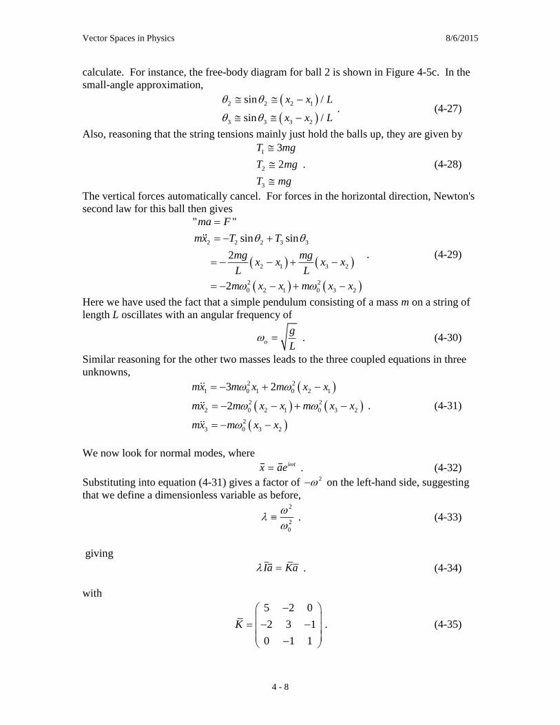
Vector Spaces in Physics 8/6/2015
4 - 8
calculate. For instance, the free-body diagram for ball 2 is shown in Figure 4-5c. In the
small-angle approximation,
2 2 2 1
3 3 3 2
sin /
sin /
x x L
x x L
. (4-27)
Also, reasoning that the string tensions mainly just hold the balls up, they are given by
1
2
3
3
2
T mg
T mg
T mg
. (4-28)
The vertical forces automatically cancel. For forces in the horizontal direction, Newton's
second law for this ball then gives
2 2 2 3 3
2 1 3 2
2 2
0 2 1 0 3 2
" "
sin sin
2
2
ma F
mx T T
mg mgx x x x
L L
m x x m x x
. (4-29)
Here we have used the fact that a simple pendulum consisting of a mass m on a string of
length L oscillates with an angular frequency of
o
g
L . (4-30)
Similar reasoning for the other two masses leads to the three coupled equations in three
unknowns,
2 2
1 0 1 0 2 1
2 2
2 0 2 1 0 3 2
2
3 0 3 2
3 2
2
mx m x m x x
mx m x x m x x
mx m x x
. (4-31)
We now look for normal modes, where
i tx ae . (4-32)
Substituting into equation (4-31) gives a factor of 2 on the left-hand side, suggesting
that we define a dimensionless variable as before,
2
2
0
. (4-33)
giving
Ia Ka . (4-34)
with
5 2 0
2 3 1
0 1 1
K
. (4-35)
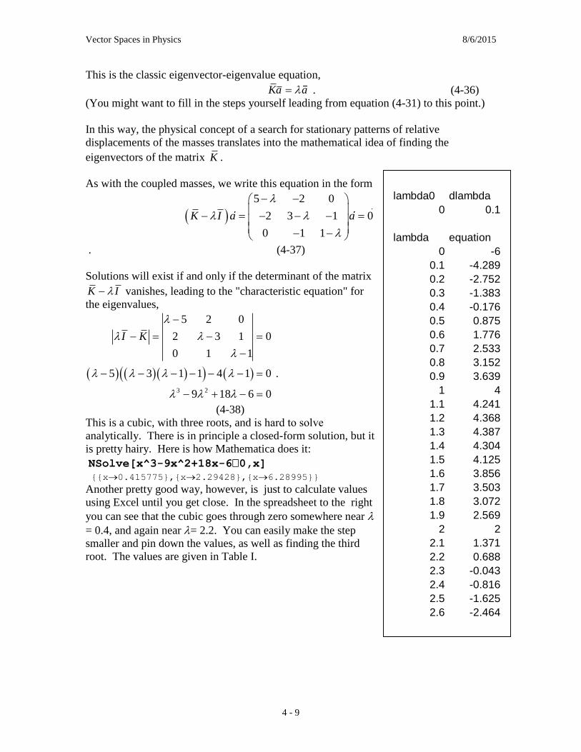
Vector Spaces in Physics 8/6/2015
4 - 9
This is the classic eigenvector-eigenvalue equation,
Ka a . (4-36)
(You might want to fill in the steps yourself leading from equation (4-31) to this point.)
In this way, the physical concept of a search for stationary patterns of relative
displacements of the masses translates into the mathematical idea of finding the
eigenvectors of the matrix K .
As with the coupled masses, we write this equation in the form
5 2 0
2 3 1 0
0 1 1
K I a a
. (4-37)
Solutions will exist if and only if the determinant of the matrix
K I vanishes, leading to the "characteristic equation" for
the eigenvalues,
3 2
5 2 0
2 3 1 0
0 1 1
5 3 1 1 4 1 0
9 18 6 0
I K
.
(4-38)
This is a cubic, with three roots, and is hard to solve
analytically. There is in principle a closed-form solution, but it
is pretty hairy. Here is how Mathematica does it:
NSolve[x^3-9x^2+18x-60,x]
{{x0.415775},{x2.29428},{x6.28995}} Another pretty good way, however, is just to calculate values
using Excel until you get close. In the spreadsheet to the right
you can see that the cubic goes through zero somewhere near
= 0.4, and again near = 2.2. You can easily make the step
smaller and pin down the values, as well as finding the third
root. The values are given in Table I.
lambda0 dlambda
0 0.1
lambda equation
0 -6
0.1 -4.289
0.2 -2.752
0.3 -1.383
0.4 -0.176
0.5 0.875
0.6 1.776
0.7 2.533
0.8 3.152
0.9 3.639
1 4
1.1 4.241
1.2 4.368
1.3 4.387
1.4 4.304
1.5 4.125
1.6 3.856
1.7 3.503
1.8 3.072
1.9 2.569
2 2
2.1 1.371
2.2 0.688
2.3 -0.043
2.4 -0.816
2.5 -1.625
2.6 -2.464

Vector Spaces in Physics 8/6/2015
4 - 10
Next, for each of the three eigenvalues, we must determine the corresponding
eigenvector. This amounts to solving the system of three homogeneous linear equations,
5 2 0
2 3 1 0
0 1 1
i
i i
i
a
. (4-39)
Here (i) and i
a are the i-th eigenvalue and eigenvector, respectively. For instance, for
the first eigenvalue given above, this gives
1
4.5842 2 0
2 2.5842 1 0
0 1 0.5842
a
. (4-40)
The magnitude of the eigenvector is not determined, since any multiple of the eigenvector
would still be an eigenvector, with the same eigenvalue. So, let's take the first
component of a to be equal to 1. The we can find the ratios a2/a1 and a3/a1 from
2
3
4.5842 2 0 1
2 2.5842 1 0
0 1 0.5842
a
a
. (4-41)
For instance, the equation from the first line of the matrix is
24.5842*1 2* 0a . (4-42)
giving
2 2.2921a . (4-43)
Next, multiply the third line in the matrix by 2.5842 and add it to the second line, to give
motion eigenvalue normalized
frequency
(single ball) 1.0000
mode 1 0.4158 0.64487
mode 2 2.2943 1.5147
mode 3 6.2899 2.5080
Table I. Eigenvalues for the three normal modes of the three-ball
system, and the corresponding frequency, given in terms of the
frequency for a single ball on a string of length L.

Vector Spaces in Physics 8/6/2015
4 - 11
2
3
4.5842 2 0 1
2 0 0.5097 0
0 1 0.5842
a
a
. (4-44)
The equation from the second line is
32 0.5097 a . (4-45)
giving
3 3.9240a . (4-46)
Or,
1
1
2.2921
3.9240
a
. (4-47)
for the first eigenvector! In this mode, the coordinates of three balls are given by
1
1 1
1
2 1
3 1
( ) cos
( ) ( ) 2.2921 cos
( ) 3.9240 cos
i t
x t t
x t x t a e t
x t t
. (4-48)
Note that the balls all move in the same direction, in this mode.
The other eigenvectors can be found in a similar way. The exact values are left to the
problems. But figure 4-6 shows the displacements of the balls in the three modes. The
higher the mode (and the higher the frequency), the more the balls move in opposite
directions.

Vector Spaces in Physics 8/6/2015
4 - 12
PROBLEMS
Problem 4-1. (a) Using identities from Appendix A, show that
0 0 0cos sin cosC t A t B t
and find A and B in terms of C and .
(b) Using identities from Appendix A, show that
00 0cos
i t i tC t De Ee
and find D and E in terms of C and . (Here C is taken to be real.)
Problem 4-2. Find the normal-mode frequencies , 1,3i i for the problem described
in the text (see fig. 4-4) of three identical masses connected by identical springs. Express
the frequencies in terms of 2
2
0
, where 0
k
m .
Problem 4-3. Find the normal modes for the problem described in the text (see figure 4-
4) of three masses connected by springs.
Problem 4-4. Consider a system of two masses and three springs, connected as shown in
figure 4-3, but with the middle spring of spring constant equal to 2k.
g g g
Figure 4-6. The three normal modes for the triple pendulum. The balls are shown at maximum
displacement, when they are all (momentarily) at rest.
Vector Spaces in Physics 8/6/2015
4 - 13
(a) Try and guess what the normal modes will be - directions of motion of the masses
and frequencies.
(b) Write the equations of motion, find the characteristic equation, and solve it, and so
determine the frequencies of the two normal modes. Compare with your guesses in part
(a).
Problem 4-5. Find the eigenvectors 2a and 3a for the triple pendulum corresponding to
the second and third eigenvalues, 2 and 2. Give a qualitative interpretation, in terms of
the co- or counter-motion of the balls, with respect to the first one.
Problem 4-6. Repeat the analysis of the multiple pendulum in the text, but for two balls,
rather than three. You should determine the two normal-mode frequencies i and the
normal-mode eigenvectors ia In this case it should be possible to find the eigenvalues
exactly, without having to resort to numerical methods. Discuss the solution.

Vector Spaces in Physics 8/6/2015
5 - 1
Chapter 5. The Inverse; Numerical Methods
In the Chapter 3 we discussed the solution of systems of simultaneous linear algebraic
equations which could be written in the form
CxA
(5-1)
using Cramer's rule. There is another, more elegant way of solving this equation, using
the inverse matrix. In this chapter we will define the inverse matrix and give an
expression related to Cramer's rule for calculating the elements of the inverse matrix. We
will then discuss another approach, that of Gauss-Jordan elimination, for solving
simultaneous linear equations and for calculating the inverse matrix. We will discuss the
relative efficiencies of the two algorithms for numerical inversion of large matrices.
A. The inverse of a square matrix.
Definition of the inverse. The inverse of a scalar number c is another scalar, say d, such
that the product of the two is equal to 1: cd=1. For instance, the inverse of the number
5 is the number 0.2 . We have defined multiplication of one matrix by another in a way
very analogous to multiplication of one scalar by another. We will therefore make the
following definition.
Definition: For a given square matrix A , the matrix B is said to be the inverse
of A if
IBAAB (5-2)
We then write 1 AB .
Notice that we have not guaranteed that the inverse of a given matrix exists. In fact,
many matrices do not have an inverse. We shall see below that the condition for a square
matrix A to have an inverse is that its determinant not be equal to zero.
Use of the inverse to solve matrix equations. Now consider the matrix equation just
given,
CxA
(5-1)
We can solve this equation by multiplying on both sides of the equation by 1A :
.
;
;
1
1
11
CAx
CAxI
CAxAA
(5-3)
Thus, knowing the inverse of the matrix A lets us immediately write down the solution
x
to equation (5-1).
As an example, let us consider a specific example, where A is a 2x2 matrix.

Vector Spaces in Physics 8/6/2015
5 - 2
5
4
11
21
;
2
1
x
x
CxA
(5-4)
If we knew the inverse of A , we could immediately calculate xAC
. In this simple
case, we can guess the inverse matrix. We write out the condition for the inverse,
ijI
IAA
??
??
**
**
11
21
;1
(5-5)
As a first guess we try to make I12 come out to zero; one possibility is
ijI
IAA
??
0?
1*
2*
11
21
;1
(5-6)
Now we arrange for I21 to be zero:
ijI
IAA
?0
0?
11
21
11
21
;1
(5-7)
If we now look at the diagonal elements of I , they come out to be I11 = 3 and I22 = -3.
We can fix this up by changing the sign of the (1,2) and (2,2) elements of the inverse, and
by multiplying it by 1/3. So we have
11
21
3
1
;10
01
11
21
3
1
11
21
;
1
1
A
I
IAA
ij (5-7)
Now that we have the inverse matrix, we can calculate the values x1 and x2:
3
2
9
6
3
1
5
4
11
21
3
1
1CAx
(5-8)
So, the solution to the two simultaneous linear equations is supposed to be x1 = -2, x2 = 3.
We will write out the two equations in long form and substitute in.
;5
4
11
21
2
1
x
x

Vector Spaces in Physics 8/6/2015
5 - 3
;53)2(
43*22
;5
42
21
21
xx
xx
55
44 .
It checks out!
The inverse matrix by the method of cofactors. Guessing the inverse has worked for a
2x2 matrix - but it gets harder for larger matrices. There is a way to calculate the inverse
using cofactors, which we state here without proof:
1cof ( )
1 ( )
ji
ij
j i
ji
AA
A
M A
A
(5-9)
(Here the minor Mpq(A) is the determinant of the matrix obtained by removing the p-th
row and q-th column from the matrix A.)
Note that you cannot calculate the inverse of a matrix using equation (5-9) if the matrix
is singular (that is, if its determinant is zero). This is a general rule for square matrices:
existnot does inverse0 A
Example: Find the inverse of the matrix
11
21A (5-10)
Here are the calculations of the four elements of 1A . First calculate the determinant:
3)2(111
21
A (5-11)
Then the matrix elements:

Vector Spaces in Physics 8/6/2015
5 - 4
;
3
11)(
;3
11)(
;3
21)(
;3
11)(
11
22
2222
1
21
21
1221
1
12
12
21
12
1
11
11
1111
1
A
A
A
AcofA
A
A
A
AcofA
A
A
A
AcofA
A
A
A
AcofA
(5-12)
So,
11
21
3
11A (5-13)
Check that this inverse works:
IAA
IAA
30
03
3
1
11
21
11
21
3
1
;30
03
3
1
11
21
11
21
3
1
1
1
(5-14)
Example: Calculate the inverse of the following 3x3 matrix using the method of
cofactors:
131
231
342
A (5-15)
Solution: This is getting too long-winded. We will just do two representative elements
of 1A .
;2
1
2
121
321
)(
;2
3
2
313
231
)(
;2)33(3)21(4)63(2
131
231
342
23
32
23
1
11
11
11
1
AA
AcofA
AA
AcofA
A
(5-16)
B. Time required for numerical calculations.

Vector Spaces in Physics 8/6/2015
5 - 5
Let’s estimate the computer time required to invert a matrix by the method of cofactors.
The quantity of interest is the number of floating-point operations required to carry out
the inverse. The inverse of a nxn matrix involves calculating n2 cofactors, each of them
requiring the calculation of the determinant of an (n-1)x(n-1) matrix. So we need to
know the number of operations involved in calculating a determinant. Let's start with a
2x2 determinant. There are two multiplications, and an addition to add the two terms.
n=2 gives 3 FLOPs. (FLOP = Floating-Point Operation.) To do a 3x3 determinant, the
three elements in the top row are each multiplied by a 2x2 determinant and added
together: 3x(3 FLOPs) + 2 FLOPs for addition; n=3 requires 3x3 + 2 FLOPs. Now we
can proceed more or less by induction. It is pretty clear that the determinant of a 4x4
matrix requires 4 calculations of a 3x3 determinant: --> 4x3x3 FLOPs. And for a 5x5
determinant, 5x4x3x3 operations. It is a pretty good approximation to say the following:
No. of operations for nxn determinant = n! (5-17)
This means that calculating the inverse by the cofactor method (n2 cofactors) requires
n2n! FLOPs.
A fast PC can today do about 10 GigaFLOPs/sec. This leads to the table given below
showing the execution time to invert matrices of increasing dimension. dim. for for inverse time (sec) for inverse time (sec)
n determinant (method of cofactors) (PC) (Gauss-Jordan) (PC)
(n!) (n^2*n!) (4n^3)
2 2 8 8E-10 32 3.2E-09
3 6 54 5.4E-09 108 1.08E-08
4 24 384 3.84E-08 256 2.56E-08
5 120 3000 0.0000003 500 0.00000005
6 720 25920 0.000002592 864 8.64E-08
7 5040 246960 0.000024696 1372 1.372E-07
8 40320 2580480 0.000258048 2048 2.048E-07
9 362880 29393280 0.002939328 2916 2.916E-07
10 3628800 362880000 0.036288 4000 0.0000004
11 39916800 4829932800 0.48299328 5324 5.324E-07
12 479001600 68976230400 6.89762304 6912 6.912E-07
13 6227020800 1.05237E+12 105.2366515 8788 8.788E-07
14 8.7178E+10 1.70869E+13 1708.694508 10976 1.0976E-06
15 1.3077E+12 2.94227E+14 29422.67328 13500 0.00000135
16 2.0923E+13 5.35623E+15 535623.4211 16384 1.6384E-06
17 3.5569E+14 1.02794E+17 10279366.67 19652 1.9652E-06
18 6.4024E+15 2.07437E+18 207436908.1 23328 2.3328E-06
19 1.2165E+17 4.39139E+19 4391388125 27436 2.7436E-06
20 2.4329E+18 9.73161E+20 97316080327 32000 0.0000032
21 5.1091E+19 2.25311E+22 2.25311E+12 37044 3.7044E-06
22 1.124E+21 5.44016E+23 5.44016E+13 42592 4.2592E-06
23 2.5852E+22 1.36757E+25 1.36757E+15 48668 4.8668E-06
24 6.2045E+23 3.57378E+26 3.57378E+16 55296 5.5296E-06
Table 5-1. Floating-point operations required for calculation of n x n determinants and
inverses of n x n matrices, and computer time required for the matrix inversion. Results

Vector Spaces in Physics 8/6/2015
5 - 6
are given for two different numerical methods. (As a useful conversion number, the
number of seconds in a year is about 3.14 x 10⁷.)
It can be seen from the table that the inversion of a 24x24 matrix could take a time on a
fast computer about equal to the age of the Universe. This suggests that a more
economical algorithm is desirable for inverting large matrices! Teasing Mathematica: Try this calculation of a determinant. n=500 m=Table[Random[],{n},{n}]; Det[m] Does this suggest that the algorithm used for Table 5-1 is not the fastest known?
C. The Gauss-Jordan method for solving simultaneous linear equations.
There is a method for solving simultaneous linear equations that avoids the determinants
required in Cramer's method, and which takes many fewer operations for large matrices.
We will illustrate this method for two simultaneous linear equations, and then for three.
Consider the 2x2 matrix equation solved above,
5
4
11
21
;
2
1
x
x
CxA
(5-4)
This corresponds to the two linear equations
5
42
21
21
xx
xx (5-18)
A standard approach to such equations would be to add or subtract a multiple of one
equation from another to eliminate one variable from one of the equations. If we add the
first equation to the second, we get
930
42
5
42
2
21eq.(2) to(1) eq.addt
21
21
x
xx
xx
xx (5-19)
Now we eliminate x2 from the top equation, by subtracting 2/3 x the bottom equation:
930
20
930
42
5
42
2
1eq.(1) from (2) eq.(2/3)x subtract
2
21eq.(2) to(1) eq. add
21
21
x
x
x
xx
xx
xx
(5-20)
And finally, multiply the second equation by 1/3:
30
20
930
20
930
42
5
42
2
11/3by (2) eq.multiply
2
1eq.(1) from (2) eq.(2/3)x subtract
2
21eq.(2) to(1) eq. add
21
21
x
x
x
x
x
xx
xx
xx
(5-21)
So we have found that x1 = -2 and x2 = 3, as determined earlier in the chapter using the
inverse.
Vector Spaces in Physics 8/6/2015
5 - 7
Note that the same operations could have been carried out using just the coefficients of
the equations, and omitting x1 and x2, as follows. The assembly of the coefficients of x1
and x2 and the constants on the right of the equation is refered to as the augmented
matrix.
3
2
10
01
9
2
30
01
9
4
30
21
5
4
11
21
1/3by (2) eq.multiply eq.(1) from (2) eq.(2.3)x subtract
eq.(2) to(1) eq. add
(5-22)
The results for x1 and x2 appear in the column to the right.
Example: Use the Gauss-Jordan method to solve the system of linear equations
represented by
4
1
1
131
231
342
;
3
2
1
x
x
x
CxA
(5-23)
Solution: We set up the augmented matrix, and then set about making the matrix part of
it diagonal, with ones on the diagonal. This is done in the following systematic fashion.
First use the first equation to eliminate A21 and A22. Next use the second equation to
eliminate A32.
3
2/1
1
100
2/110
342
2/7
2/1
1
2/110
2/110
342
4
1
1
131
231
342
(3) from (2)subtract
(3) from and (2) from (1) x 1/2subtract
(5-24)
Next we work upwards, using equation (3) to eliminate A23 and A13. After that, equation
(2) is used to eliminate A12. At this point the matrix is diagonal. the final step is to
multiply equations (1) and (3) by a constant which makes the diagonal elements of A
become unity.

Vector Spaces in Physics 8/6/2015
5 - 8
3
2
1
100
010
001
3
2
2
100
010
002
3
2
10
100
010
042
3
2/1
1
100
2/110
342
1-by (3) and 1.2by (1)multiply
(1) from (2) x 4subtract
(1) to(3) * 3 add(2), to(3) * 1./2 add
(5-25)
The solution for the unknown x's is thus x1 = 1, x2=2, x3 = -3.
SUMMARY: Work your way through the matrix, zeroing the off-diagonal elements, IN
THE ORDER SHOWN BELOW, zeroing ONE, then TWO, then THREE, etc. If you try
to invent your own scheme of adding and subtracting rows, it may or may not work.
.
THREETWO
FOURONE
FIVESIX
D. The Gauss-Jordan method for inverting a matrix.
There is a very similar procedure which leads directly to calculating the inverse of a
square matrix. Suppose that B is the inverse of . Then
100
010
001
;
333231
232221
131211
333231
232221
131211
BBB
BBB
BBB
AAA
AAA
AAA
IBA
(5-26)
This can be thought of us three sets of three simultaneous linear equations:
,
1
0
0
,
0
1
0
,
0
0
1
33
23
13
333231
232221
131211
32
22
12
333231
232221
131211
31
21
11
333231
232221
131211
B
B
B
AAA
AAA
AAA
B
B
B
AAA
AAA
AAA
B
B
B
AAA
AAA
AAA
(5-27)
These three sets of equations can be solved simultaneously, using a larger augmented
equation, as follows:
A

Vector Spaces in Physics 8/6/2015
5 - 9
110
2/12/12/1
2/12/52/3
100
010
001
110
2/12/12/1
153
100
010
002
110
2/12/12/1
331
100
010
042
110
012/1
001
100
2/110
342
102/1
012/1
001
2/110
2/110
342
100
010
001
131
231
342
1-by (3) and 1/2by (1)multiply
(1) from (2) x 4subtract
(1) to(3) * 3 add(2), to(3) * 1./2 add
(3) from (2)subtract
(3) from and (2) from (1) x 1/2subtract
(5-28)
So, the result is
220
111
153
2
11AB (5-29)
The check is to multiply by its inverse:
100
010
001
200
020
002
2
1
131
231
342
220
111
153
2
1AB (5-29)
So the inverse just calculated is correct.
Time for numerical inverse. Let us estimate the time to invert a matrix by this
numerical method. The process of zeroing out one element of the left-hand matrix
requires multiplying the line to be subtracted by a constant (2n FLOPs), and subtracting it
(2n FLOPs). This must be done for (approximately) n2 matrix elements. So the number
of floating-point operations is about equal to 4n3 for matrix inversion by the Gauss-
Jordan method. Consulting Table 5-1 shows that, for a 24x24 matrix, the time required
is less than a milli-second, comparing favorably with 1011 years for the method of
cofactors.
Number of operations to calculate the inverse of a nxn matrix.
method number of FLOPs
cofactor n2*n!
Gauss-Jordan 4n3
PROBLEMS
Problem 5-1. (a) Use the method of cofactors to find the inverse of
the matrix
A

Vector Spaces in Physics 8/6/2015
5 - 10
111
111
111
C .
(b) Check your result by verifying that ICC 1 .
Problem 5-2. Use the Mathematica function Inverse to find the inverse of the matrix
111
111
111
C .
(See Appendix C for the necessary Mathematica operations.) Check your result.
Problem 5-3. Prove that if an operator A has both a left inverse (call it B ) and a right
inverse (call it C ), then they are the same; that is, if
IAB and
ICA
then
CB .
[Be careful to assume only the properties of B and C that are given above. It is not to
be assumed that A , B and C are matrices.]
Problem 5-5. Suppose that B and C are members of a group with distributive
multiplication defined, each having an inverse (both left-inverse and right-inverse). Let
A be equal to the product of B and C , that is,
CBA .
Now consider the group member D , given by 1 1D C B .
Show by direct multiplication that D is both a left inverse and a right inverse of A .
[Be careful to assume only the properties of B and C that are given above. It is not to
be assumed that A , B and C are matrices.]
Problem 5-6. (a) Use the method of Gauss-Jordan elimination to find the inverse of the
matrix
111
101
111
C .
(b) Check your result by verifying that ICC 1 .

Vector Spaces in Physics 8/6/2015
6 - 1
Chapter 6. Rotations and Tensors
There is a special kind of linear transformation which is used to transforms coordinates
from one set of axes to another set of axes (with the same origin). Such a transformation
is called a rotation. Rotations have great practical importance, in applications ranging
from tracking spacecraft to graphical display software. They also play a central role in
theoretical physics
The linear transformation corresponding to a rotation can be described by a matrix. We
will describe the properties of rotation matrices, and discuss some special ones.
A. Rotation of Axes.
In chapter 1 we considered a rotation
of a Cartesian coordinate system
about the z-axis by an angle . A
more general case is shown in figure
6-1, where the axes are transformed
by rotation into an arbitrary second
set of axes. (We take both sets or
axes to be right handed.
Transformation to a left-handed
coordinate system is to be avoided,
unless you really know what you are
doing.) A typical vector A
is also
shown.
Figure 6-2 (a) shows the components
of A
in the )ˆ,ˆ,ˆ( 321 eee system, and
figure 6-2 (b) shows its coordinates in the )'ˆ',ˆ',ˆ( 321 eee system. We see that we can write
A
, using components in the unprimed system, as
i iA e A ; (6-1)
or, using components in the primed frame, as
ˆ ' 'i iA e A (6-2)
The standard definitions of components are clear from (6-1) and (6-2):
ˆ ,
ˆ' ' .
i i
i i
A e A
A e A
(6-3)
We can, however, relate the primed components to the unprimed, as follows:
x
x'
y'
z'
z
y
'1e1e2e
3e'ˆ
2e'ˆ
3e
A
Figure 6-1. Two sets of Cartesian coordinate axes.
The (x',y',z') system is obtained from the (x,y,z)
system by a rotation of the coordinate system.

Vector Spaces in Physics 8/6/2015
6 - 2
ˆ' '
ˆ ˆ' ( )
ˆ ˆ'
jj
j l l
j l l
jl l
A e A
e A e
e e A
C A
(6-4)
That is to say that the relationship between primed and unprimed components can be
expressed as a matrix equation,
ACA
' , (6-5)
where the transformation matrix C is given by
ˆ ˆ( ' )jjl lC C e e . (6-6)
There is an interpretation of the coefficients Cjl in terms of angles. Since all of the ˆje
and le are unit vectors, the dot product of any two is equal to the cosine of the angle
between them:
'
ˆ ˆ' cosm n m ne e . (6-7)
Example: Consider a rotation by an angle in the counter-clockwise sense about the z
axis, as described in Chapter 1. Since the z axis is the same in the primed and unprimed
systems, certain of the coefficients ˆ ˆ'jjl lC e e are especially simple:
0 C C C C
1, C
23133231
33
; (6-8)
The other coefficients can be read off from figure (2-4):
x
z
y 11Ae
A
x
x'
y'
z'
z
y
'1e1e2e
3e'ˆ
2e'ˆ
3e
A
22ˆ Ae
33 Ae
(a) (b) 33Ae
22ˆ Ae
11Ae
Figure 6-2. The vector A
expressed in terms of its )ˆ,ˆ,ˆ( 321 eee components (a), and in terms of its
)'ˆ',ˆ',ˆ( 321 eee components (b).

Vector Spaces in Physics 8/6/2015
6 - 3
.sin-i'j C
,sinj'i C
,cosj'j C
,cosi'i C
21
12
22
11
; (6-9)
and so
)(
100
0cossin
0sincos
zRC
. (6-10)
The matrices corresponding to rotations about the x and y axes can be calculated in a
similar way; the results are summarized below.
1 0 0
( ) 0 cos sin
0 sin cos
cos 0 sin
( ) 0 1 0
sin 0 cos
cos sin 0
( ) sin cos 0
0 0 1
x
y
z
R
R
R
. (6-11)
B. Some properties of rotation matrices.
Orthogonality. Consider the definition of the transformation matrix C :
ˆ ˆ( )jjl lC C e e . (6-6)
If we form the product of C and its transpose, we get
ˆ ˆ ˆ ˆ' '
ˆ ˆ ˆ ˆ' '
T T
im mlil
im lm
m mi l
m mi l
CC C C
C C
e e e e
e e e e
. (6-12)
But, the vector l
e , like any vector, can be written in terms of its components in the un-
primed frame,
ˆ ˆ ˆ ˆ( )m ml le e e e . (6-13)
In this sum, ˆ ˆ( )m le e is the m-th component of the vector
le in the unprimed frame. So,
equation (6-12) becomes

Vector Spaces in Physics 8/6/2015
6 - 4
ˆ ˆ' 'T
i lil
il
CC e e
. (6-14)
or
ICC T . (6-15)
The equivalent statement in index notation is
ij lj ilC C . (6-15a)
A similar calculation for the product TC C leads to
T
li lj il
C C I
C C
. (6-15b)
This leads us to define orthogonality as follows:
[Note: We have not used the condition that either ˆ , 1,3ie i or ˆ , 1,3ie i form a right-
handed coordinate system, so orthogonal rotations include both rotations and
transformations consisting of a rotation and a reflection. More about this distinction
later.]
Example: Show that the rotation matrix of (6-10) above is orthogonal.
Solution:
I
CC T
100
0cossincossincossin
0cossincossinsincos
100
0cossin
0sincos
100
0cossin
0sincos
22
22
. (6-16)
Determinant. It is easy to verify the following fact: The determinant of an orthogonal
matrix must be equal to either +1 or -1. (The proof is left to the problems.) If its
determinant is equal to +1, it is said to be a proper orthogonal matrix. All rotation
matrices are proper orthogonal matrices, and vice versa. Rotation matrices must have a
determinant of +1. However, this is not the only condition for a square matrix to be a
rotation matrix. It must also have the property that its transpose is equal to its inverse.
For an orthogonal matrix, the
transpose matrix is also the inverse
matrix. T T
li lj il jl il
C C CC I
C C C C
(6-15c)
Vector Spaces in Physics 8/6/2015
6 - 5
NOTE: All rotation matrices are orthogonal; but not all orthogonal matrices are
rotation matrices. Can you explain why?
C. The Rotation Group
Rotations are linear operators which transform three coordinates {xi} as seen in one
coordinate system into three coordinates {x'i} in another system. All vectors transform in
this same way, as given in equation (6-4) above:
'j jl lA C A (6-4)
We have shown that C must be orthogonal, and have determinant equal to +1.
Multiplication of two rotation matrices gives another square matrix, and it must also be a
rotation matrix, since carrying out two rotations, one after another, can be represented by
a single rotation. So, the rotation group is defined as follows.
Definition. The "rotation group" consists of the set of real orthogonal 3x3 matrices with
determinant equal to +1.
(a) Group multiplication is just matrix multiplication according to the standard
rules.
(b) The group is closed under multiplication.
(c) The identity matrix is the identity of the group.
(d) For every element A of the group, there exists an element A-1, the inverse of
A, such that 1AA I .
(e) Multiplication satisfies A BC AB C .
These properties are easy to prove and are left to the exercises.
D. Tensors
What are tensors? Tensors look like matrices; but only certain types of matrices are
tensors, as we shall see. They must transform in a certain way under a rotation of the
coordinate system. Vectors, with one index, are tensors of the first rank. Other objects,
such as the rotation matrices themselves, may have more than one index. If they
transform in the right way, they are considered to be higher-order tensors. We will first
discuss rotations, then define tensors more precisely.
Under a rotation of the coordinate system, the components of the displacement vector
x change in the following way:
iji j= .x xR (6-17)
The tensor transformation rules represent a generalization of the rule for the
transformation of the displacement vector.
Tensors of Rank Zero. A rank-zero tensor is an object g which is invariant under
rotation:
Rank - zero tensor : g g (6-17a)

Vector Spaces in Physics 8/6/2015
6 - 6
Tensors of Rank One. Modeled on the rotation properties of vectors, we define a
tensor of rank one as an object with a single index, iC ={ ,i =1,3}C or just Ci for short,
such that the components Ci' in a rotated coordinate system are given by
i ij jFirst - Rank Tensor : C = C .R (6-18)
Tensors of Rank Two. A second-rank tensor is an object with two indices,
1,3}=ji,,D{=D ij or Dij for short, such that its components Dij' in a rotated coordinate
system are given by
Second - Rank Tensor: D = R R D .ij ik jl kl (6-19)
That is to say, each of the two indices transforms like a single vector index.
Tensors of Rank Three. Following the same pattern, a third-rank tensor Hijk follows
the transformation law
ijk il jm kn lmnThird - Rank Tensor : = .H R R R H (6-19)
And so on.
Much of the power of tensor analysis lies in the ease in which new tensors can be
created, with their transformation properties under rotations just determined by the
number of tensor indices. Here are two theorems about creation of tensors which we
offer without proof.
Tensor Products: The direct product of a tensor of rank n and a tensor of rank m
is a tensor of rank n+m.
Thus, for instance, the product of two vectors, AiBj, is a second-rank tensor.
Contraction of Indices: If two tensor indices are set equal (and so summed), the
resulting object is a tensor of rank lower by two than that of the original tensor.
Example: Let us consider the contraction of the two indices of the tensor AiBj:
i iA B A B .
(6-20)
The fact that this dot product is a zero-rank tensor guarantees that it has the same
value in all coordinate systems.
Special Tensors. The Kronecker delta symbol and the Levi-Civita symbol have
indices which look like tensor indices - but their components are defined to be the same
regardless of the coordinate system. Can they still transform like tensors, of rank two and
three, respectively? This is in fact the case; the proof is left for the problems. This
means that these two tensors can be used in conjunction with vectors and other tensors to
make new tensors.

Vector Spaces in Physics 8/6/2015
6 - 7
Example: Consider the following tensor operations: First form the direct
product ijkAlBm of the Levi-Civita tensor with two vectors A and B. Then
perform two contractions of indices, by setting l=j and m=k. This produces the
following object, with one free index:
l j
j kijkijk l m im kA B (AxB )A B
. (6-21)
This is what we call the cross product or vector product. The theorems about
tensor indices guarantee, since it has one free index, that it does in fact transform
like a vector under rotations.
Example: The trace and determinant of a tensor are both scalars, since all the
free tensor indices are removed by contraction. Thus, the trace and determinant
of a matrix are the same in all coordinate systems, provided that the matrix itself
transforms like a tensor.
E. Coordinate Transformation of an Operator on a Vector Space.
Here is an explanation of the transformation law for a second-rank tensor. Consider an
operator O operating on a vector A to produce another vector B :
B OA . (6-22)
Tensors are all about looking at something from another point of view - in a rotated
coordinate system. So, if we write quantities in the rotated coordinate system with a
prime, the other point of view is
B O A . (6-23)
Under rotations, every vector is just multiplied by R . If we apply this to both sides of
equation (6-22) it becomes
RB R OA . (6-24)
Now insert between O and A a factor of the identity matrix, which we can write as 1 TI R R R R , where we have used the fact that R's inverse is just its transpose.
T
T
RB ROA
ROR RA
ROR RA
. (6-25)
This just shows the operator working in the rotated coordinate system, as shown in
(6.23), provided that the operator in the rotated coordinate system is given by
TO ROR .Similarity Transformation (6-26)
This process, of sandwiching a square matrix between R and its inverse, is called a
similarity transformation.
But . . . shouldn't O transform like a second-rank tensor? Let's write 6-26) in tensor
notation,
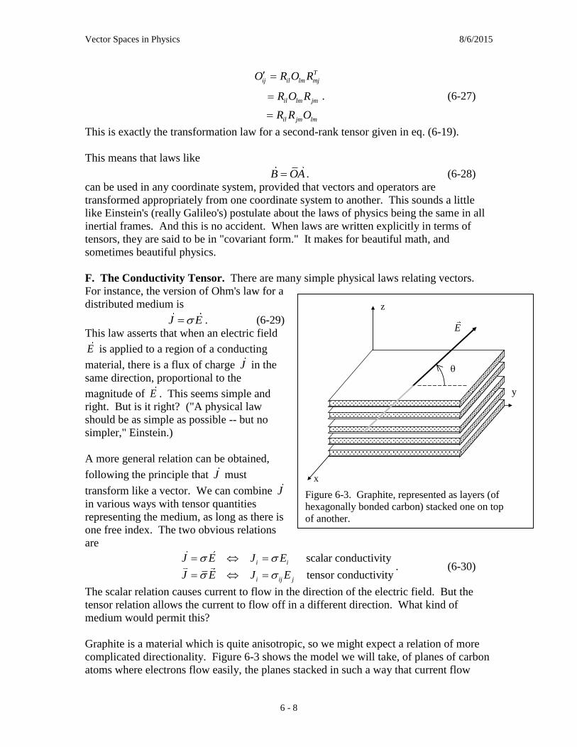
Vector Spaces in Physics 8/6/2015
6 - 8
T
ij il lm mj
il lm jm
il jm lm
O R O R
R O R
R R O
. (6-27)
This is exactly the transformation law for a second-rank tensor given in eq. (6-19).
This means that laws like
B OA . (6-28)
can be used in any coordinate system, provided that vectors and operators are
transformed appropriately from one coordinate system to another. This sounds a little
like Einstein's (really Galileo's) postulate about the laws of physics being the same in all
inertial frames. And this is no accident. When laws are written explicitly in terms of
tensors, they are said to be in "covariant form." It makes for beautiful math, and
sometimes beautiful physics.
F. The Conductivity Tensor. There are many simple physical laws relating vectors.
For instance, the version of Ohm's law for a
distributed medium is
J E . (6-29)
This law asserts that when an electric field
E is applied to a region of a conducting
material, there is a flux of charge J in the
same direction, proportional to the
magnitude of E . This seems simple and
right. But is it right? ("A physical law
should be as simple as possible -- but no
simpler," Einstein.)
A more general relation can be obtained,
following the principle that J must
transform like a vector. We can combine J
in various ways with tensor quantities
representing the medium, as long as there is
one free index. The two obvious relations
are
scalar conductivity
tensor conductivity
i i
i ij j
J E J E
J E J E
. (6-30)
The scalar relation causes current to flow in the direction of the electric field. But the
tensor relation allows the current to flow off in a different direction. What kind of
medium would permit this?
Graphite is a material which is quite anisotropic, so we might expect a relation of more
complicated directionality. Figure 6-3 shows the model we will take, of planes of carbon
atoms where electrons flow easily, the planes stacked in such a way that current flow
x
y
z
E
Figure 6-3. Graphite, represented as layers (of
hexagonally bonded carbon) stacked one on top
of another.

Vector Spaces in Physics 8/6/2015
6 - 9
from one plane to another is more difficult. We can set up a conductivity matrix as
follows. From symmetry, we would expect that an electric field in the x-y plane would
cause a current in the direction of E , with conductivity 0 "in the planes." And, also
from symmetry, an electric field in the z direction should cause current to flow in the z
direction, but with a much smaller conductivity 1. This can be written in matrix form as
0 1
0 2
1 3
0 0
0 0
0 0
E
J E E
E
. (6-31)
If you multiply this out, you see that the first two components of E (the x and y
components) are multiplied by 0, and the third component, by 1.
But what if for some reason it is better to use a rotated set of axes? Then the applied field
and the conductivity tensor both need to be transformed to the new coordinate system,
and their product will produce the current density in the new coordinate system. Note
that scalar quantities, like J E , are zero-th rank tensors and should have the same value
in both coordinate systems.
Numerical Example. In equation (6-31), let's take 1 = 0.1 * 0 (weak current
perpendicular to the graphite planes) and have the electric field in the y-z plane, at an
angle of 45 from the y axis, as shown in figure (6-3):
0 0
01 0 0
2, 0 1 0
20 0 0.1
2
2
E E
. (6-32a)
This gives for the current density J in the original coordinate system,
0 0 0 0
0 01 0 0
2 20 1 0
2 20 0 0.1
2 2
2 20
J E E E
. (6-32b)
The z component of the current is small compared to the y component, and so the current
vector moves closer to the plane of good conduction.
Now let's see what happens in a rotated coordinate system. Let's go to the system where
the electric field is along the z axis. This requires a rotation about the x axis of 45 .
Using the form of this matrix given in eq. (6-11) above, we have

Vector Spaces in Physics 8/6/2015
6 - 10
1 0 0
2 2( 45 ) 0
2 2
2 20
2 2
xR R
. (6-33)
In this system the electric field vector is simpler:
0 0
1 0 0 00
2 2 20 0
2 2 21
2 2 20
2 2 2
E RE E E
; (6-34)
And the conductivity tensor becomes
0
0
0
1 0 0 1 0 01 0 0
2 2 2 20 0 1 0 0
2 2 2 20 0 0.1
2 2 2 20 0
2 2 2 2
1 0 0 1 0 0
2 2 2 20 0
2 2 2 2
2 2 2 20 0
2 2 20 20
1 0 0
0 0.55 0.45
0 0.45 0.55
TR R
; (6-35)
Now here is the punch line: We can either rotate J (calculated in the original coordinate
system) into the rotated coordinate system; or we can calculate it directly, using the
electric field and the conductivity tensor expressed in the rotated coordinate system.
Here goes:

Vector Spaces in Physics 8/6/2015
6 - 11
0 0 0 0
1 0 0 00
2 2 20 0.45
2 2 20.55
2 2 20
2 2 20
J RJ E E
; (6-36)
And the other way:
0 0 0 0
1 0 0 0 0
0 0.55 0.45 0 0.45
0 0.45 0.55 1 0.55
J E E E
; (6-36)
It works - same result either way. Here is the interpretation of this example.
The equation
J E
produces the current density flowing in a medium (a vector) in terms of the electric field
in the medium (also a vector). But . . . the current does not necessarily flow in the
direction of the applied electric field. The most general vector result caused by another
vector is given by the operation of a second-rank tensor!
In a simple physics problem, the conductivity tensor will have a simple form, in a
coordinate system which relates to the structure of the material. But what if we want to
know the current flowing in some other coordinate system? Just transform the applied
field and the conductivity tensor to that coordinate system, and use
J E
G. The Inertia Tensor.
In classical mechanics, a rigid body which is
rotating about its center of mass had angular
momentum. The rate of rotation at a particular
instant of time can be described by a vector, ,
which is in the direction of the axis of rotation, with
magnitude equal to the angular speed, in
radians/sec. The angular momentum is also given
by a vector, L , which is equal to the sum (or
integral) of the individual angular momenta of the parts of the rigid body, according to
dL dm r v . (6-37)
In certain cases, such as when the rotation is about an axis of symmetry of the object, the
relation between L and is simple:
L I . (6-38)
x
x
x
r
v
L
Figure 6-4. Displacement and velocity,
and the resulting angular momentum.

Vector Spaces in Physics 8/6/2015
6 - 12
Here I is the moment of inertia discussed in a first
course in mechanics.
However, surprisingly enough, the resultant total
angular momentum vector L is not in general parallel
to . The general relation involves an angular-
momentum tensor, I , rather than the scalar moment
of inertia. The general relation is
L I . (6-
39)
where now, for a body approximated by N discrete point masses,
1
N
i
i
L L
and (6-39)
i i i iL m r v
is the angular momentum of the i-th mass. The velocity of a point in the rotating body is
given by
i iv r ,
and so
dL dm r v
dm r r
We will evaluate the double cross product using tensor notation and the epsilon killer.
i i
ijk j klm l m
kij klm j l m
il jm im jl j l m
dL dm r r
dm r r
dm r r
dm r r
dm
(6-41)
Problems
The Pauli matrices are special 2x2 matrices associated with the spin of particles like the
electron. They are
10
01,
0
0,
01
10321
i
i.
(Here “i” represents the square root of -1.)
Problem 6-1. (a) What are the traces of the Pauli matrices?
(b) What are the determinants of the Pauli matrices?
(c) Are the Pauli matrices orthogonal matrices? Test each one
v r
r
Figure 6-5. A rigid body, rotating about
an axis through the origin.

Vector Spaces in Physics 8/6/2015
6 - 13
Problem 6-2. The Pauli matrices are claimed to satisfy the relation
2j k k j jkl li
Test this relation, for j=2, k=3.
Problem 6-3. In Problem 6-1 above one of the Pauli matrices, 2
0
0
i
i
, did not
turn out to be orthogonal. For matrices with complex elements a generalized relationship
must be used: † † is CC C C I C unitary
where the "Hermetian conjugate" matrix †C is the complex conjugate of the transpose
matrix.
(a) Calculate the Hermetian conjugate †
2 of the second Pauli matrix.
(b) Check and see if it is unitary.
[Unitary matrices become important in quantum mechanics, where one cannot avoid
working with complex numbers.]
Problem 6-5. Using the fact that the determinant of the product of two matrices is the
product of their determinants, show that the determinant of an orthogonal matrix must be
equal to either +1 or -1. Hint: Start with the orthogonality condition TA A I .
Problem 6-6. For each of the three matrices below, say whether or not it is orthogonal,
and whether or not it is a rotation matrix. Justify your answers.
2
20
2
2
0102
20
2
2
,
500
043
034
5
1,
001
010
100
CBA
Problem 6-7. Consider rotations Rx() and Rz(), with the matrices Rx and Rz as defined
in the text. Here represents the angle of a rotation about the x axis and represents the
angle of a rotation about the z axis.
First, calculate the matrices representing the result of carrying out the two rotations in
different orders:
zx RRA
and
xz RRB .
Comparing A and B , do you find that the two rotations xR and zR commute?
Vector Spaces in Physics 8/6/2015
6 - 14
Next, look at your results in the small-angle approximation (an approximation where
you keep only terms up to first order in the angles and ). Does this change your
conclusion?
Problem 6-8. Show algebraically that the rotation group is closed under multiplication.
that is, show that, for A and B members of the rotation group, the product matrix C = AB
is orthogonal and has determinant equal to +1.
Problem 6-10. The Kronecker delta symbol is defined to have constant components,
independent of the coordinate system. Can this be true? That is to say, is it true that ?
il jmij lm ij R R
Use the orthogonality of the transformation matrix Rij to show that this is true.
Problem 6-11. The Levi-Civita symbol ijk, defined previously, has specified constant
values for all of its components, in any frame of reference. How can such an object be a
tensor - that is, how can these constant values be consistent with the transformation
properties of tensor indices? Well, they are! Consider the transformation equation
where R is a rotation matrix, satisfying the orthogonality condition RijRik = jk, and ijk is
the Levi-Civita symbol. The question is, does ' have the same values for all of its
components as ? As a partial proof (covering 21 of the 27 components), prove that
0ijk = if any two of the indices {i,j,k} are equal.
Note: in carrying out this proof, set two indices to the same value - but do not sum over
that index. This operation falls outside of the Einstein summation convention.
Problem 6-12 Tensor transformation of the Levi-Civita symbol. (Challenge
Problem) Prove that under transformations of tensor indices by an orthogonal matrix R,
the Levi-Civita tensor transforms according to the rule
detijk ijk= ( R ) .
Problem 6-13 Invariance of length under rotation. The length of a vector is a scalar,
and so should not change from one coordinate system to another. To check this, use the
vectors E and J from the conductivity example in the text. See if they have the same
magnitude in both coordinate systems used.
Problem 6-14 Invariance of a scalar product under rotation. The inner product of
two vectors is a scalar, and so should not change from one coordinate system to another.
To check this, use the vectors E and J from the numerical example in the discussion of
tensor conductivity in this chapter. See if the inner product E J is the same in both
coordinate systems used.
,RRR= lmnknjmilijk

Vector Spaces in Physics 8/6/2015
6 - 15
Problem 6-15. Return to the numerical example in the discussion of tensor conductivity
in this chapter. Suppose that the electric field E in the original system still has
magnitude E0, but is directed along the positive z axis; that is,
0
0
0E
E
(a) Calculate the current density J E in the unprimed system.
(b) Now consider the same rotation, using R from the example in the text, and calculate
J E in the primed system. (Note: has already been calculated in the notes.)
(c) Now calculate the current density in the primed system by the alternate method,
J RJ . Compare with the result from part (b).

Vector Spaces in Physics 8/6/2015
6a - 1
Chapter 6a. Space-time four-vectors.
The preceding chapters have focused on a description of space in terms of three
independent, equivalent coordinates. Here we discuss the addition of time as a fourth
coordinate in "space-time." This leads to the consideration of space-time
transformations, or Lorentz transformations, which are an extension to four dimensions
of rotations in three dimensions. Special relativity is introduced here as a generalization
of the invariance of length under rotations in three-space. The transformation of the
Maxwell stress tensor under relativistic "boosts" is introduced as an application to
electromagnetic theory. A later chapter, intended to follow the study of Maxwell's
equations, shows how covariant tensor calculus leads to these equations.
A. The origins of special relativity.
This course is mainly about mathematical methods, so I will completely ignore the rich
history of scientific discovery and speculation that lead to the integration of space and
time into four-space. I will just go over the most compelling reasons based on modern
science for requiring something like special relativity.
1. There are lots of kinds of electromagnetic radiation known: light, radio waves, X-
rays, WiFi and microwave ovens. All of these disturbances travel at a certain special
speed, c = 3 x 10⁸ m/s.
2. Beams of electrons are commonplace. Electrons in radio and television tubes respond
like most massive particles, speeding up in response to forces acting on them. However,
at particle accelerators such as SLAC, it is observed that as particles approach the speed
c, they are harder and harder to speed up. They never quite get up to speed c.
3. Radioactive particles are also commonplace; they decay with a characteristic half life.
But, mu mesons which are contained in circular orbit by a magnetic field live longer than
when at rest. Furthermore, the light curves of supernovae moving away from us at high
velocity are stretched out in time, indicating that decaying iron and nickel isotopes are
exhibiting a longer half life, presumably because they are moving with a speed
approaching c.
Note that c is a special property of nature, even for phenomena which have nothing to do
with light. However, we always call it "the speed of light."
So - it is not too dumb to propose the following: we have admired the simplicity of
coordinate transformations from one frame of reference to a rotated frame. Space
coordinates are changed, but time is not involved. However, the phenomena described
above suggest that a moving observer sees time differently. We thus suppose that
transforming to the point of view of a moving observer involves a special sort of
"rotation" in space and time.
B. Four-vectors and invariant proper time.

Vector Spaces in Physics 8/6/2015
6a - 2
We will add a time coordinate to the usual 3-component space vector. Time does not
have the correct units - but ct (time multiplied by the speed of light) does. Thus we have
a four-vector:
z
y
x
ct
x (6a-1)
[Note about indices. I will use Greek letters such as , , , and (mu, nu, lambda and
ksi) to label space-time components, as distinct from i, j, k, l . . . for space components.
There is also an issue about upper and lower indices, corresponding to contra-variant and
co-variant indices. I will try to avoid discussing their difference in detail, leaving that for
a more specialized course.] A space-time index takes on one of the four values 0, 1, 2, 3.
Thus x1, x2, and x3 are just the usual x, y, and z, with the fourth coordinate as x0 = ct.
Now, what do we do with a four-vector? An important property of a three-space vector is
its length. For a vector
1
2
3
A
A A
A
, the length 2A A is given by
2
2 2 2
1 2 3
ij i jA A A
A A A
(6a-2)
For the special case of the position vector r , the scalar length r is given by
2
2 2 2
1 2 3
ij i jr x x
x x x
(6a-3)
We recall that under rotation the components x1, x2, and x3 can change, but in such a way
that the length r is invariant. In fact, orthogonal transformations are defined to be just
those linear coordinate transformations which leave the length of vectors invariant.
In space-time, the corresponding length is called proper time . It is defined this way:
2
c g x x
(6a-4)
where g is the metric tensor, defined as follows:
1 0 0 0
0 1 0 0
0 0 1 0
0 0 0 1
g
(6a-5)
This gives, in terms of the common variables t, x, y, and z,
2 2 2 2 2c g x x ct x y z
(6a-6)
This is bit more complicated than the three-space version. For one thing, the inner
product is formed using not the Kronecker delta function ij, but the metric tensor g.
Note that it has two lower indices. A general rule for using four-space indices is the
Vector Spaces in Physics 8/6/2015
6a - 3
following: When carrying out a contraction by setting two indices equal, one must be a
lower index and the other, an upper index. The Einstein summation convention is of
course in force, where a paired index is assumed to be summed, from 0 to 3.
There is one major difference between the length of a three-vector and the length of a
four-vector. Because of the minus sign in the metric tensor, the length of the vector can
come out to be zero, or even negative. This is a warning that, while time has been
introduced as a vector component, it is really still different from the space components.
C. The Lorentz transformation.
The defining property of a three-vector is how it changes when the frame of reference (of
the observer) is rotated about an axis. The corresponding change in the frame of
reference for a 4-vector is from that of a "stationary" observer to that of an observer
moving with velocity v in a particular direction, usually taken to be the x-direction. (See
figure 6a-1.) What is the transformation which changes space and time coordinates, in
such a way as to leave the 4-vector length unchanged? Here it is - the Lorentz
transformation.
0 0
0 0The Lorentz Transformation
0 0 1 0
0 0 0 1
(6a-7)
where
2
1
1
(6a-8a)
and
v
c (6a-8b)
These symbols form the language of relativity. The symbol is often just referred to as
the velocity; it is a dimensionless velocity formed by dividing the actual velocity (the
relative velocity of the two frames of reference) by the speed of light. The two symbols
and are functions of the velocity . They play the role for the Lorentz
transformation that cos and sin play in the rotation zR ; instead of
2 2cos sin 1 we have
2 2 1 (6a-9)
The role of the Lorentz transformation matrix
given above is to calculate four-space
coordinates in a "moving" coordinate system S' , in terms of those in a "stationary"

Vector Spaces in Physics 8/6/2015
6a - 4
system S. These systems are illustrated below in figure 6a-1.
The frame S' is in motion, relative to S, with velocity v in the x-direction. The Lorentz
transformation from S to S' is
1
1 1
2 2
3 3
0 0
0 0
0 0 1 0
0 0 0 1
ct ct x
x ct xx x
x x
x x
(6a-10)
or, in the form often quoted for the Lorentz transformation,
2'
'
'
'
vt t x
c
x x vt
y y
z z
(6a-11)
The inverse of this transformation is pretty easy to figure out. It is just obtained by
changing v to -v. is unchanged, and changes to -,giving
1
0 0
0 0The Inverse Lorentz Transformation
0 0 1 0
0 0 0 1
(6a-12)
and
x
y
z
t
S
x
'
y
'
z
'
t
'
S'
v
'
Figure 6a-1. Two rest-frames, in relative motion.
Vector Spaces in Physics 8/6/2015
6a - 5
1 11
2 2
3 3
0 0
0 0
0 0 1 0
0 0 0 1
ct ct
x xx x
x x
x x
(6a-13)
D. Space-time events.
Some of the most interesting effects in special relativity involve objects in motion - that
is, in motion with respect to the observer. The frame of reference in which the object is
not in motion is called its rest frame. Properties of an object, in space or time, may vary
according to the observer's state of motion with respect to the object, and the properties
observed in the rest frame are considered to be fundamental properties of the object. For
instance, the intrinsic length of an object is that measured in its rest frame. And the time
for an object to do something (go to sleep, then wake up, for instance) is properly
measured in the object's rest frame. We will now show that time intervals are stretched
out ("dilated") if the object is moving, and lengths are shortened ("contracted").
The basis of geometry in three-space consists of points, specified by the coordinates
(x,y,z). In four-space we talk instead of events, specified by time and position, e.g., for
event A,
A
A
A
A
A
ct
xx
y
z
. (6a-14)
A point in space can be marked by driving a stake in the ground, or carving your name on
a tree. For a four-space version, some authors imagine setting off a small bomb, so that a
black mark gives the position, and the sound adds the time. It is of special interest to
consider the 4-space displacement between two events. Thus, the displacement from
event A to event B is
B A
B A
B A
B A
B A
c t t
x xx x x
y y
z z
. (6a-15)
E. The time dilation.
Let us consider two events, A and B, happening to an object in frame S'. This is the rest
frame of the particle, so they both happen at a single point, which we will take to be the
origin, x' = y' =z' = 0. Let the first event happen at time t = 0, and the second, at time
T0. So, the four-vector positions of A and B, in frame S', are

Vector Spaces in Physics 8/6/2015
6a - 6
0 00
0 0 0, , and .
0 0 0
0 0 0
A B B A
cT cT
x x x x x
Now we use the inverse Lorentz transformation to go to the frame S of the observer:
0 0
01
0 0
0 0 0
0 0 1 0 0 0
0 0 0 1 0 0
cT cT
cTx x
(6a-16)
This tells us that the time interval T observed in S is a factor of greater than the time
interval T0 observed in the rest frame. That is,
0T T time dilation (6a-17)
Example. Suppose a rocket going to Mars travels at relativistic speed 0.1 ,
that is, at 10% the speed of light. (This is not actually very practical.) How long
would a year of an astronaut's life (observed in her rest frame, moving with the
rocket) appear to take?
The time-dilation factor is
2
1 11.005
1 0.011
So, the length of the dilated year (as we see it, not in her rest frame) is
0 1.005 yearsT T .
F. The Lorentz contraction.
According to the Lorentz contraction, fast-moving objects appear shorter than they
actually are. Let us see how this works. Suppose that a stick of length L0 (if measured in
its rest frame S') is in fact observed in frame S, where it appears to be moving at velocity
v along the x-axis. Let events A and B be observations of the two ends of the stick in its
rest frame, as shown in figure 6a-2 below.

Vector Spaces in Physics 8/6/2015
6a - 7
Events A and B are separated by a distance L0, the length of the stick. We do not require
them to be at the same time, since the stick is not moving. So we can take A to be at the
origin, at time t' = 0, and event B to be at the end of the stick, at undetermined time t'B.
Thus,
0 0
0
0, , and x = .
0 0 0
0 0 0
B B
A B B A
ct ct
L Lx x x x
.
We use the inverse Lorentz transformation to see the length of the stick in frame S:
0
0 01
0 0
0 0
0 0 1 0 0 0
0 0 0 1 0 0
B B
B
ct ct L
L ct Lx x
(6a-18)
We are interested in events A and B which occur at the same time in frame S. And with
this condition, the separation of events A and B in frame S is the length of the stick, as
observed with the stick in motion. That is,
0
0
0
0 0
0 0
B
B
ct L
ct L Lx
(6a-19)
This gives two equations, for the first two components. The first one can be used to
eliminate tB, giving
x'
y'
z'
t' S'
A B
L0
Figure 6a-2. Two events A and B as seen in system S'. They
mark observations (not necessarily simultaneous) of the two
ends of a stick of length L0.

Vector Spaces in Physics 8/6/2015
6a - 8
0Bt Lc
,
and then the second equation gives
0
0 0
2 20
BL t L
L Lc
L
or, using 2 2 1 ,
0
1L L
Lorentz contraction (6a-20)
G. The Maxwell field tensor.
The electric field E and the magnetic field B each have three components which
seem to be related to the directions in space. But how do they fit into relativistic four-
space? There are no obvious scalar quantities to provide the fourth component of their
four-vectors. Furthermore, the magnetic field has some dubious qualities for a true
vector. For one, it is derived from a cross product of vectors, and so does not reverse
under the parity transformation, as all true vectors do.
There is another interesting argument indicating that the relativistic transformation
properties of the electric and magnetic fields are complicated. Under Lorentz
transformation, the four components of the four-vector are re-arranged amongst
themselves. But the transformation to a moving coordinate system turns a pure electric
field into a combination of electric and magnetic fields. This can be understood in a very
rough way from the following observation. An electrostatic field can be produced by a
distribution of fixed charges. But if one shifts to a moving coordinate system, the
charges are moving, constituting currents, which generate magnetic fields.
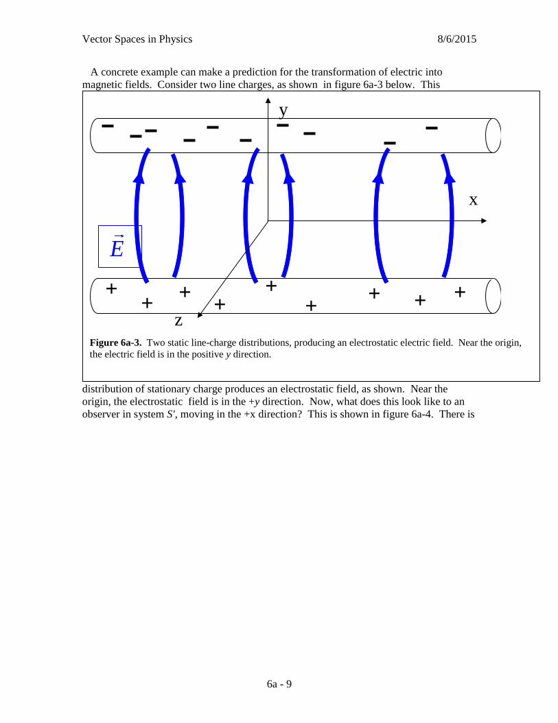
Vector Spaces in Physics 8/6/2015
6a - 9
A concrete example can make a prediction for the transformation of electric into
magnetic fields. Consider two line charges, as shown in figure 6a-3 below. This
distribution of stationary charge produces an electrostatic field, as shown. Near the
origin, the electrostatic field is in the +y direction. Now, what does this look like to an
observer in system S', moving in the +x direction? This is shown in figure 6a-4. There is
+ + +
+ + + + + +
E
x
y
z
Figure 6a-3. Two static line-charge distributions, producing an electrostatic electric field. Near the origin,
the electric field is in the positive y direction.

Vector Spaces in Physics 8/6/2015
6a - 10
now a magnetic field, in the negative z direction. There is another, more subtle
prediction. Because of the Lorentz contraction, the wires appear shorter, and so the
charge density on the wires is greater, and the electric field should be stronger.
So, we have this prediction for the transformation of electromagnetic fields: Suppose
that there is just an electric field present in S, in the positive y-direction. Then in the S'
frame, the field transformation should produce a magnetic field in the negative z-
direction, and a stronger electric field, still in the positive y-direction. Now we will
postulate a transformation law for electromagnetic fields, and see if this prediction is
fulfilled.
Here is the field-strength tensor of special relativity.
+ + +
+ + + + + +
E
x'
y'
z'
I
I B
B B B
B B
E E
Figure 6a-4. Two linear distributions of charges moving in the -x-direction, producing both an electrostatic
electric field and a magnetic field.. Near the x-axis, the magnetic resulting from the two "wires" is in the -z'-
direction.

Vector Spaces in Physics 8/6/2015
6a - 11
0
0
0
0
x y z
x z y
y z x
z y x
E E E
E B BF
E B B
E B B
(6a-21)
The electric and magnetic fields are seen to be components of a four-tensor, rather than
forming parts of four-vectors. This may seem more complicated than necessary. As I.I.
Rabi said on hearing about the mu meson, who asked for that? Well, we know how to
transform a tensor into a moving frame of reference; and so we can see what a simple
electric field looks like to a moving observer.
The tensor transformation works just like with three-vectors and rotations R , except
that the Lorentz transformation matrix
plays the role for four-tensors that R played
for three-tensors. The electromagnetic fields as seen in the moving system are thus
0
0
0
0
00 0 0 0
00 0 0 0
00 0 1 0 0 0 1 0
00 0 0 1 0 0 0 1
0 0
0 0
x y z
x z y
y z x
z y x
T
x y z
x z y
y z x
z y x
E E E
E B BF
E B B
E B B
F
F
E E E
E B B
E B B
E B B
2 2
2 2
00 0 1 0
00 0 0 1
0
0
0
0
x x y z
x x z y
y z y z x
z y z y x
x y z z y
x y z z y
y z y z x
z y z y x
E E E E
E E B B
E B E B B
E B E B B
E E B E B
E E B E B
E B E B B
E B E B B
(6a-22)
And finally, using the relation 2 2 1 , we have a grand result:
Vector Spaces in Physics 8/6/2015
6a - 12
0
0
0
0
x y z z y
x y z z y
y z y z x
z y z y x
E E B E B
E E B E BF
E B E B B
E B E B B
(6a-23)
Let's try to absorb this result. To start with, note that the matrix is still anti-symmetric;
this is a cross check on the algebra. Next, we see that the x-components of both E and
B , in the direction of the relative velocity, do not change. However, for the transverse
fields, they get all scrambled up. We can write the four non-trivial field transformation
equations like this:
y y z
z z y
y y z
z z y
E E B
E E B
B B E
B B E
(6a-24)
We see that the transverse components of both fields get bigger. This is what we
predicted for the E field. And a bit of the other field, in the other transverse direction,
gets added on. Here is another simple check. Take the zero-velocity limit. Do you find
that the fields do not change?
Finally, let's consider the example above. We predicted that transforming a positive Ey
would give a negative Bz. Look at the fourth equation above: that is just what happens.
I. I. Rabi would love it.
Note on units: The form of F
given is in Gaussian units. To use SI units, replace
iE by /iE c .
Problems
Problem 6a-1. The algebra of special relativity leans heavily on the following
dimensionless symbols:
2
1
1
v
c
Here v represents the velocity of one frame of reference with respect to the other.
(a) What are the limiting values of these three symbols as the velocity v approaches the
speed of light c?
(b) Calculate the value of 2 2
The result should be independent of the velocity.

Vector Spaces in Physics 8/6/2015
6a - 13
(c) The inverse of the Lorentz boost
0 0
0 0
0 0 1 0
0 0 0 1
is obtained by reversing the velocity v, which causes the change . The result is
given above, in equation (6a-12). Carry out the matrix multiplication to demonstrate that
this works; that is, show by direct calculation that 1 I
Problem 6a-2. The magnitude of the 4-position vector,
2 2 2 2ct x y z ,
should be invariant under Lorentz transformation. Using the relations given in equation
(6a-11) above, calculate
2 2 2 2ct x y z
and see if the invariance works out.
Problem 6a-3. The energy of an object at rest is (famously) given by 2E mc , where m
(as always in our discussions) represents the object's rest mass. And, in the object's rest
frame, its four-momentum
x
y
z
E
p cp
p c
P c
(general case)
becomes 2
0
0
0
mc
p
(in the particle's rest frame).
(a) Set the invariant length-squared of the first expression above equal to the invariant
length-squared of the second one. Solve for the object's energy E, in terms of its
momentum p and its rest-mass m. (The speed of light, c, will be there too.)
(b) Multiply the second four-vector by the Lorentz-transformation matrix 1 (that is,
transform it to a frame of reference moving backwards along the x-axis, with velocity
) and use the result to derive expressions for the object's energy and momentum as a
function of the relativistic velocity of the particle.
Problem 6a-4. The nearest star to our sun is about 3 light-years away. That is,
something traveling from Earth at speed v = c would take 3 years to get to the star,
according to observers in the Earth frame of reference. Consider a rocket, carrying an

Vector Spaces in Physics 8/6/2015
6a - 14
astronaut, traveling to the star from Earth at speed . The time T to get there would be
3 yearsT
.
(a) How fast would the rocket have to travel, in m/sec, to get to the star within a
reasonable life expectancy of the astronaut, say T0 = 50 years? (Start by calculating the
value of .) Note: here you can approximate 1 , so astronaut time and Earth time
will be about the same.
(b) Answer the same question about travel to Andromeda, 1,500,000 light-years away,
also in 50 years of astronaut time. Note: in calculating the travel time in the Earth frame
you can approximate 1 , so that the travel time in the Earth frame is about 1,500,000
years.
Problem 6a-5. Recent studies of distant supernovae played a central role in the
discovery of dark energy. One researcher (Prof. Gerson Goldhaber) pointed out that the
relativistic time dilation should be observable for the most distant galaxies, which are
moving close to the speed of light. This is because the decrease in the brightness of a
supernova over the first 100 days after the initial explosion is due to the decaying of the
isotope Fe58, which decays with a half-life of 20 days. According to the theory of special
relativity, this half-life should appear longer to us. (The half-life is the time for the decay
rate to decrease by a factor of 1/2.)
If the galaxy is moving with speed 0.8 , how long should it take for its light to
decrease in intensity by a factor of 1/2? By a factor of 1/128?

Vector Spaces in Physics 8/6/2015
7 - 1
Chapter 7. The Wave Equation
The vector spaces that we have described so far were finite dimensional. Describing position in
the space we live in requires an infinite number of position vectors, but they can all be represented
as linear combinations of three carefully chosen linearly independent position vectors. There are
other analogous situations in which a complicated problem can be simplified by focusing attention
on a set of basis vectors. In addition to providing mathematical convenience, these basis vectors
often turn out to be interesting objects in their own right.
The pressure field inside a closed cylindrical tube (an ''organ pipe'') is a function of time and three
space coordinates which can vary in almost an arbitrary way. Yet there are certain simple patterns
which form a basis for describing all
the others, and which are
recognizably important and
interesting. In this case they are the
fundamental resonance of the organ
pipe and its overtones. They are the
''notes'' which we use to make music,
identified by our ears as basis vectors
of its response space. A similar
situation occurs with the vibrating strings of guitars and violas (or with the wires strung between
telephone poles), where arbitrary waves moving on the string can be represented as a superposition
of functions corresponding again to musical notes.
Another analogous situation occurs with quantum- mechanical electron waves near a positively
charged nucleus. An arbitrarily complicated wave function can be described as a linear
superposition of a series of ''states,'' each of which corresponds (in a certain sense) to one of the
circular Bohr electron orbits.
We will choose the stretched
string to examine in
mathematical detail. It is the
easiest of these systems to
describe, with a reasonable set
of simplifying assumptions.
The mathematical variety that it
offers is a rich preview of
mathematical physics in
general.
A. Qualitative properties
of waves on a string
Many interesting and
intellectually useful experiments can be carried out by exciting waves on a stretched string, wire or
n = 1
n = 2
Figure 7-2. Modes of resonance of a vibrating string.
Figure 7-1. A pulse traveling down a telephone wire (solid
curve), and a reflected pulse traveling back (dashed curve).
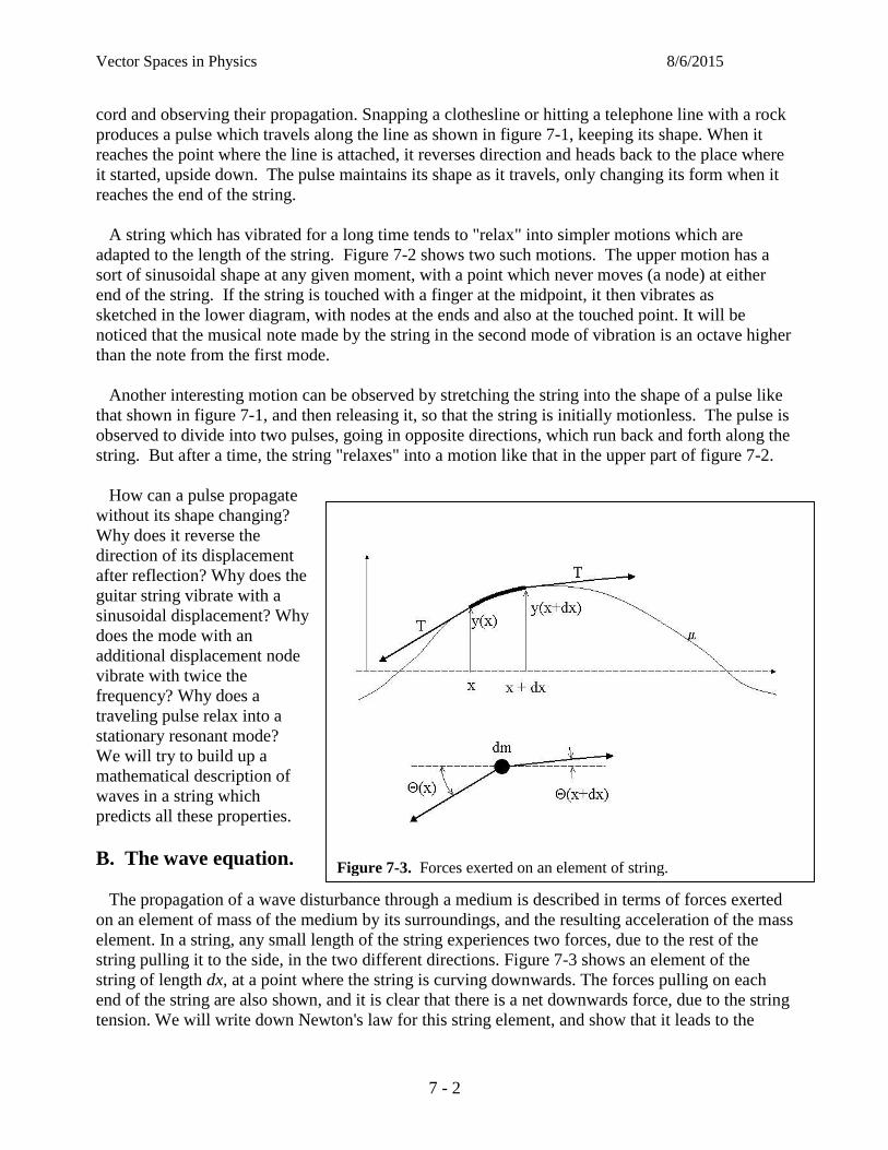
Vector Spaces in Physics 8/6/2015
7 - 2
cord and observing their propagation. Snapping a clothesline or hitting a telephone line with a rock
produces a pulse which travels along the line as shown in figure 7-1, keeping its shape. When it
reaches the point where the line is attached, it reverses direction and heads back to the place where
it started, upside down. The pulse maintains its shape as it travels, only changing its form when it
reaches the end of the string.
A string which has vibrated for a long time tends to "relax" into simpler motions which are
adapted to the length of the string. Figure 7-2 shows two such motions. The upper motion has a
sort of sinusoidal shape at any given moment, with a point which never moves (a node) at either
end of the string. If the string is touched with a finger at the midpoint, it then vibrates as
sketched in the lower diagram, with nodes at the ends and also at the touched point. It will be
noticed that the musical note made by the string in the second mode of vibration is an octave higher
than the note from the first mode.
Another interesting motion can be observed by stretching the string into the shape of a pulse like
that shown in figure 7-1, and then releasing it, so that the string is initially motionless. The pulse is
observed to divide into two pulses, going in opposite directions, which run back and forth along the
string. But after a time, the string "relaxes" into a motion like that in the upper part of figure 7-2.
How can a pulse propagate
without its shape changing?
Why does it reverse the
direction of its displacement
after reflection? Why does the
guitar string vibrate with a
sinusoidal displacement? Why
does the mode with an
additional displacement node
vibrate with twice the
frequency? Why does a
traveling pulse relax into a
stationary resonant mode?
We will try to build up a
mathematical description of
waves in a string which
predicts all these properties.
B. The wave equation.
The propagation of a wave disturbance through a medium is described in terms of forces exerted
on an element of mass of the medium by its surroundings, and the resulting acceleration of the mass
element. In a string, any small length of the string experiences two forces, due to the rest of the
string pulling it to the side, in the two different directions. Figure 7-3 shows an element of the
string of length dx, at a point where the string is curving downwards. The forces pulling on each
end of the string are also shown, and it is clear that there is a net downwards force, due to the string
tension. We will write down Newton's law for this string element, and show that it leads to the
Figure 7-3. Forces exerted on an element of string.

Vector Spaces in Physics 8/6/2015
7 - 3
partial differential equation known as the wave equation. But first, we will discuss a set of
approximations which makes this equation simple.
First, we will make the small-angle approximation, assuming here that the angle which the string
makes with the horizontal is small ( 1 ). In this approximation, cos 1 and sin .
Secondly, we will assume that the tension T is constant throughout the string. Two of these
assumptions ( cos 1 and T constant) result in a net force of zero in the longitudinal (x) direction,
so that the motion of the string is purely transverse. We will ignore a possible small longitudinal
motion and assume that it would have only a small effect on the transverse motion which we are
interested in.
In the transverse (y) direction, the forces do not cancel. The transverse component of the force on
the left-hand side of the segment of string has magnitude T sin . We will relate sin to the slope
of the string, according to the relation from analytic geometry
rise
slope tan sinrun
dy
dx . (7-1)
The last, approximate, equality is due to the small-angle approximation. Thus the transverse force
has magnitude approximately equal to dy
Tdx
, and Newton's second law for the transverse motion
gives
2
2
y
x dx x
F dm a
y y yT T dx
x x t
(7-2)
Here we have used the linear mass density (mass per unit length) to calculate dm = dx.
Partial derivatives.
In the equation above we replaced the slope dy
dx by
y
x
, a partial derivative. We need to explain
briefly the difference between these two types of derivatives.
The displacement of the string is a function of two variables, the position x along the string, and
the time t. There are two physically interesting ways to take the derivative of such a function. The
rate of change of y with respect to x, at a fixed instant of time, is the slope of the string at that time,
and the second derivative is related to the curvature of the string. Similarly, the rate of change of y
with respect to time at a fixed position gives the velocity of the string at that point, and the second
time derivative gives the acceleration. These derivatives of a function with respect to one variable,
while holding all other variables constant, are referred to as partial derivatives.
The partial derivatives of an arbitrary function g(u,v) of two independent variables u and v are
defined as follows:
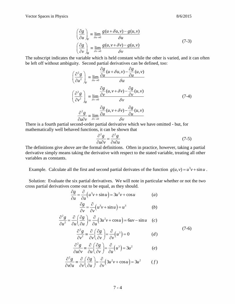
Vector Spaces in Physics 8/6/2015
7 - 4
0
0
( , ) ( , )lim
( , ) ( , )lim
u
v
v
u
g g u u v g u v
u u
g g u v v g u v
v v
(7-3)
The subscript indicates the variable which is held constant while the other is varied, and it can often
be left off without ambiguity. Second partial derivatives can be defined, too:
2
2 0
2
2 0
2
0
( , ) ( , )
lim
( , ) ( , )
lim
( , ) ( , )
lim
u
v
v
v
u
g gu u v u v
g u u
u u
g gu v v u v
g v v
v v
g gu v v u v
g u u
u v v
(7-4)
There is a fourth partial second-order partial derivative which we have omitted - but, for
mathematically well behaved functions, it can be shown that
2 2g g
u v v u
(7-5)
The definitions give above are the formal definitions. Often in practice, however, taking a partial
derivative simply means taking the derivative with respect to the stated variable, treating all other
variables as constants.
Example. Calculate all the first and second partial derivates of the function 3( , ) sing u v u v u .
Solution: Evaluate the six partial derivatives. We will note in particular whether or not the two
cross partial derivatives come out to be equal, as they should.
3 2
3 3
22
2
23
2
23 2
22 2
sin 3 cos ( )
sin ( )
3 cos 6 sin ( )
0 ( )
3 ( )
3 cos 3 (
gu v u u v u a
u u
gu v u u b
v v
g gu v u uv u c
u u u u
g gu d
v v v v
g gu u e
u v u v u
g gu v u u
v u v u v
)f
(7-6)
Vector Spaces in Physics 8/6/2015
7 - 5
Check the two cross partial derivatives. Sure enough, 2 2g g
u v v u
.
Wave velocity.
Now we will work out the partial differential equation resulting from Newton's second law.
Starting with equation 7-2, we get
2
2
x dx x
y y
yx x
dx T t
(7-7)
But we recognize the left-hand side as just the definition of the second partial derivative with
respect to x, provided we let dx be arbitrarily small:
2
20lim x dx x
dx
dy dy
ydx dx
dx x
(7-8)
And so we get the differential equation for the string, also known as the wave equation:
2 2
2 2
y y
x T t
(7-9)
It is easy to see that the dimensions of the two constants must be such that a characteristic velocity
v can be defined as follows:
T
v
(7-10)
In terms of this characteristic velocity, the differential equation becomes
2 2
2 2 2
1y y
x v t
The Wave Equation (7-11)
Now we must find the solutions to this partial differential equation, and find out what it is that
moves at speed v.
C. Sinusoidal solutions.
Since we associate the sinusoidal shape with waves, let's just try the function
( , ) siny x t A kx t (7-12)
At a fixed time (say, t = 0), this function (shown in figure 7-4) describes a
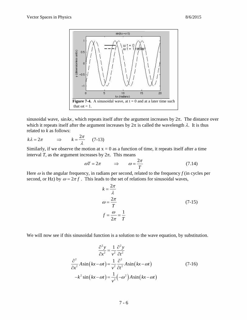
Vector Spaces in Physics 8/6/2015
7 - 6
sinusoidal wave, sin kx , which repeats itself after the argument increases by 2. The distance over
which it repeats itself after the argument increases by 2 is called the wavelength . It is thus
related to k as follows:
22k k
(7-13)
Similarly, if we observe the motion at x = 0 as a function of time, it repeats itself after a time
interval T, as the argument increases by 2. This means
2
2TT
(7.14)
Here is the angular frequency, in radians per second, related to the frequency f (in cycles per
second, or Hz) by 2 f . This leads to the set of relations for sinusoidal waves,
2
2
1
2
k
T
fT
(7-15)
We will now see if this sinusoidal function is a solution to the wave equation, by substitution.
2 2
2 2 2
2 2
2 2 2
2 2
2
1
1sin sin
1sin sin
y y
x v t
A kx t A kx tx v t
k kx t A kx tv
(7-16)
Figure 7-4. A sinusoidal wave, at t = 0 and at a later time such
that t = 1.

Vector Spaces in Physics 8/6/2015
7 - 7
The factor of sin kx t cancels out on both sides, and it is clear that the sine wave is a solution
to the wave equation only if k and are related in a certain way:
vk T
(7-17)
If we adopt this relation, we can write the sine wave in the following equivalent ways:
sin sin 2 sinx t
kx t k x vtT
(7-18)
Example: Consider transverse waves on the lowest string of a guitar (the E string). Let us
suppose that the tension in the string is equal to 300 N (about 60 lbs), and that the 65-cm-long
string has a mass of 5 g (about the weight of a nickel). The fundamental resonance of this string
has a wavelength equal to twice the length of the string. Calculate the mass density of the string
and the speed of transverse waves in the string. Also calculate f, and k for this resonance.
Solution: The mass density is
0.005 kg
0.65 m
0.00769 kg/m
m
L
(7-19)
The wave speed is then
2300 kg-m/s
0.00769 kg/m
197.5 m/s
Tv
(7-20)
For a wavelength of = 1.3 m we get
-1
-1
2 24.833 m
1.3 m
4.833 m 197.5 m/s 954 rad/sec
152 Hz2
k
kv
f
(7-21)
Is this right for an E string? Using a frequency of 440 Hz for A above middle C, an A two octaves
down would have a frequency of (440 Hz)/4 = 110 Hz, and the E above that note would be at f =
(110 Hz)*1.5 = 165 Hz. [An interval of an octave corresponds to a factor of two in frequency; a
fifth, as between A and E, corresponds to a factor of 1.5.]
So, the frequency of the E string is a bit low. What do you do to correct it? Check the equations
to see if tightening the string goes in the right direction.

Vector Spaces in Physics 8/6/2015
7 - 8
Example. Water waves are a type of transverse wave, propagating along the water surface. A
typical speed for waves traveling over the continental shelf (water depth of 40 m) is v = 20 m/s. If
the wavelength is = 220 m, find the frequency and period with which a buoy will bob up and
down as the wave passes. Also calculate and k.
Solution. With the velocity and wavelength known, the period of the oscillation and the
frequency can be calculated:
220 m11 sec
20 m/s
10.091 Hz
Tv
fT
(7-22)
If you want to see if this period is reasonable, go to the web site
http://facs.scripps.edu/surf/nocal.html and look at "the swells" off the coast right now.
And and k.
-1
2 0.571 rad/sec
2 20.0286 m
220 m
f
k
(7-23)
As a cross check, see if /k gives back the wave speed; this is an important relation.
0.571 rad/sec
20 m/s0.0286 mk
(7-24)
It works out.
D. General traveling-wave solutions.
It is heartening to have guessed a solution to the wave equation so easily. But how many other
solutions are there, and what do they look like? Is a sine wave the only wave that travels along at
speed v, without changing its form?
In fact, it is easy to see that a huge variety of waves have this property. [However, later on we
will see that the wave keeps its shape intact only if the wave speed does not depend on the
wavelength.] Consider any function whose argument is x vt ,
( , ) ( )y x t f x vt (7-30)
We can take two partial derivatives with respect to x and two partial derivatives with respect to t,
using the chain rule, and see what happens.
( )f x vt f x vt x vtx x
f x vt
(7-31)

Vector Spaces in Physics 8/6/2015
7 - 9
Here f' is the derivative of the function f with respect to its argument. Taking the second partial
derivative with respect to x gives
2
2( )f x vt f x vt
xx
f x vt x vtx
f x vt
(7-32)
Taking the time derivative is similar, except
that in place of 1x vtx
, we have
x vt vt
. So,
( )f x vt f x vt x vtt t
vf x vt
(7-33)
and
2
2
2
( )f x vt vf x vttt
vf x vt x vtt
v f x vt
(7-34)
Substituting into the wave equation shows it to be satisfied:
2 2
2 2 2
2
2
1
1
y y
x v t
f x vt v f x vtv
f x vt
(7-35)
As an illustration, let's consider the Gaussian function
2
22( )
u
g u e
shown in figure 7-5. We
can use this function to interpret the meaning of the parameter v in the wave equation. The peak of
the Gaussian occurs when the variable u is equal to zero. Suppose the argument of the function is x
- vt instead of u:
2
22( )
x vt
g x vt e
(7-36)
At t = 0, the peak of the function occurs when x = 0. But at a later time t = t, the peak as a
function of position will occur at a value x such that the argument x v t vanishes; this gives
0 wave velocityx
x v t vt
(7-37)
Figure 7-5. Gaussian wave form, with = 1.

Vector Spaces in Physics 8/6/2015
7 - 10
Thus, the velocity with which the peak of the Gaussian appears to move is just the constant v which
occurs in the wave equation. From now on, we will refer to it as the wave velocity.
E. Energy carried by waves on a string.
One of the paradoxical aspects of wave motion has to do with the question of what exactly about
the wave is moving. The string itself does not move in the direction of wave propagation. It seems
to be just the shape, or the profile made by the displaced string, which moves. But it can be seen
that there is energy in the moving string, and an argument can be made that energy is transported
by the wave, in the direction of the wave propagation.
Kinetic energy.
It is rather clear that there is kinetic energy due to the transverse motion associated with the
displacement y x v t . Referring to figure 7-6a, we can see that the kinetic energy of the
string between x and x+dx is given by
2
2
1 ( , )KE
2
1 ( , )
2
y x td dm
t
y x tdx
t
(7-38)
Potential energy.
The potential energy due to the displacement of the string from the equilibrium position is equal
to the work done in stretching an undisplaced string out to the position of the string at a given
instant of time. Figure 7-6b shows how this calculation proceeds. We will write the displacement
of the string at this instant of time as y(x,t0), where the subscript on t0 reminds us that this time is
held fixed. We imagine exerting at every point on the string just the force necessary to hold it in
position. Then gradually the string is stretched from a straight line out to its shape y(x,t0) at time t0.
Let 0,x a f x t be the displacement of the string during this process. As the parameter
goes from 0 to 1, the string displacement goes from 0x to 0( , )x y x t .
In deriving the wave equation we calculated the force on a length dx of the string, due to the
tension T and the curvature of the string:
2
2
y
x dx x
x dx x
y yF T
x x
y y
x xTdx
dx
yTdx
x
(7-39)

Vector Spaces in Physics 8/6/2015
7 - 11
When the displacement is equal to 0( , )y x t , the force will be equal to 2
2
yTdx
x
. We now
calculate the work done on length dx of the string as goes from 0 to 1.
1
0
1
0
0
1 2
2
0
12
2
0
2
2
,
. ( , )
1
2
y
y
W F x d
F x y x t d
yTdx yd
x
yTdx y d
x
yT y dx
x
(7-40)
Thus we have, for a general wave motion y(x,t),
Figure 7-6. Graphs of a traveling wave. The upper curve (a) shows an element of mass on the string and its
transverse velocity. The lower curve (b) shows the virtual process of stretching a string from the equilibrium
position to its actual position at an instant of time, to facilitate calculating the work done in this virtual process.
Vector Spaces in Physics 8/6/2015
7 - 12
2
2
2
1KE per unit length =
2
1PE per unit length = -
2
y
t
yT y
x
(7-41)
Example. Calculate the kinetic, potential and total energy per unit length for the sinusoidal
traveling wave
( , ) siny x t A kx t (7-42)
Solution. We will use the relations (7-33). The KE per unit length is
2
2 2 2
1KE per unit length sin
2
1cos
2
A kx tt
A kx t
; (7-43)
and the PE per unit length is
2
2
2
2
2
2 2 2
2 2 2
1PE per unit length
2
1sin sin
2
1sin sin
2
1sin
2
1sin
2
yTy
x
T A kx t A kx tx
T A kx t k A kx t
Tk A kx t
A kx t
; (7-44)
In the last step we have used the relations kv (general for all sinusoidal waves) and T
v
(waves on a string). Note the similarity of the expressions for the two types of energy. The only
difference is the presence of the factor of 2cos kx t in one case, and 2sin kx t in the
other. If we use the well-known property that either sin2 u or cos2 u averages to 1/2 when averaged
over a large number of cycles, we see that the average energy per unit length is the same in the two
modes of energy storage, and we have
2 2
time time
1KE per unit length PE per unit length
4Tk A . (7-45)
Here the brackets time represent an average over time. The equality of the average energy in
these two types of energy is an example of a situation often found in physics where different
"degrees of freedom" of a system share equally in the energy. Note that the average could have
been carried out over position x along the string rather than the time, and the result would have
been the same.
The total energy per length is constant, since 2 2sin cos 1kx t kx t , for any time or
position along the string:

Vector Spaces in Physics 8/6/2015
7 - 13
2 2 2 2
Total Energy per unit length KE per unit length+PE per unit length
1 1= =
2 2Tk A A
(7-46)
Example. Consider the E string on a guitar as discussed in a previous example, with T = 300 N,
= 0.00769 kg/m, k = 4.833 m-1, and = 954 rad/sec. Take the amplitude of the string's deflection
to be A = 1 cm, and calculate the average energy density for kinetic and potential energy, and the
total energy in the string.
Solution. Just plug into the previous relations.
2 2
2 2
Average KE per unit length Average PE per unit length
1=
4
1= 0.00769 kg/m 954 rad/sec 0.01 m
4
0.175 J/m
A
(7-47)
The total energy density is twice this, giving for the total energy
total energy total energy density length of string
0.350 J/m 0.65 m
=0.228 J
(7-48)
This isn't much. If the note dies away in one second, the maximum average audio power would be
a quarter of a watt. Aren't guitars louder than that? Oops - what's that great big black box on stage
beside the guitar?
F. The superposition principle.
There is a very important property of linear differential equations, like the wave equation, called
the superposition principle, which can be stated as follows for the wave equation:
The Superposition principle. Suppose that 1 ,f x t and 2 ,f x t are two solutions to the
wave equation as given above. Then any linear combination ,g x t of f1 and f2, of the
form
1 2( , ) , ,g x t f x t f x t , (7-49)
where and are arbitrary constants, is also a solution to the wave equation.
This is pretty easy to prove. First we calculate the partial derivatives:
2 2
1 22 2
2 2
1 2
2 2
, ,g
f x t f x tx x
f f
x x
(7-50)
and
Vector Spaces in Physics 8/6/2015
7 - 14
2 2
1 22 2 2 2
2 2
1 2
2 2 2 2
1 1, ,
1 1
gf x t f x t
v t v t
f f
v t v t
(7-51)
Now substitute into the wave equation, in the form
2 2
2 2 2
10
y y
x v t
(7-52)
For ,g x t this becomes
2 2
2 2 2
2 2 2 2
1 2 1 2
2 2 2 2 2 2
10 ?
1 10 ?
g g
x v t
f f f f
x x v t v t
(7-53)
Regrouping, we have
2 2 2 2
1 1 2 2
2 2 2 2 2 2
2 2 2 2
1 1 2 2
2 2 2 2 2 2
1 10 ?
1 10 ? YES!!!
f f f f
x v t x v t
f f f f
x v t x v t
(7-54)
Since f1 and f2 each satisfies the wave equation, the two expressions in parentheses vanish
separately, and the equality is satisfied.
This principle gives us a great deal of freedom in constructing solutions to the wave equation. A
very common approach to wave problems involves representing a complicated wave solution as the
superposition of simpler waves, as illustrated in the next section.
G. Dispersion; Group and phase velocity.
The wave equation with constant coefficients as given by equation (7-11) has traveling-wave
solutions which all travel at the same speed. This is true for sinusoidal solutions (equation (7-12))
or for arbitrarily shaped pulses (equation (7-30)). A wave medium where this is the case is referred
to as a "non-dispersive" medium, for the following reason: while sinusoidal waves propagate
without changing their shape, wave pulses do not; in general, as a wave pulse propagates, it
changes its shape, in most cases getting broader and broader as it travels. This broadening is
referred to as dispersion.
In a dispersive medium, there are two important velocities to be considered. The "phase
velocity," which we have represented with the symbol v, is the velocity of a sinusoidal wave of a
certain frequency or wavelength. The other velocity is the "group velocity," which we will denote
by u. The group velocity has the following definition, which will really only be clear after we have
discussed Fourier series and transforms. A pure sinusoidal solution to the wave equation represents
a disturbance which is completely delocalized, in the sense that it has the same amplitude for all
positions on the string and for all times. If one wanted to represent a short light signal from a laser,
for instance, as used in communications, it would make sense to use a modified wave which has a

Vector Spaces in Physics 8/6/2015
7 - 15
beginning and an end. In order to do this, a linear superposition of sinusoidal waves of different
wavelengths can be used. However, this means superposing waves traveling at different velocities!
If they are initially lined up so as to add up to give a narrow pulse, or "wave packet," it makes sense
that after some time elapses they will no longer be properly aligned. The result of such a process of
superposition, however, is that the wave packet moves at a velocity which is entirely different from
the velocity of the component sinusoidal waves!
(the group velocity) (the phase velocity)u v (7-55)
This remarkable fact has to be seen to be believed. There is a rather simple example of
superposition of waves which illustrates it. Let's superimpose two sinusoidal waves of equal
amplitude A, and slightly different wave numbers 1 0k k k and 2 0k k k . that is, the two
wave numbers are separated by an amount 2 k , and centered about the value k0. We will assume
that we know the "dispersion relation:"
( ) the dispersion relationk (7-56)
For non-dispersive media where v is a constant, this is a very simple linear relation, kv ,
obtained from equation (7-17). However, if v is a function of k, the relation becomes more
complicated. In any event, this relation allows the angular frequencies 1 0 and
2 0 to be determined from k1 and k2. We now carry out the superposition.
1 1 2 2
0 0 0 0
, sin sin
sin sin
y x t A k x t A k x t
A k x t kx t A k x t kx t
(7-57)
Now we use the trigonometric identities
sin sin cos cos sin
sin sin
cos cos
a b a b a b
b b
b b
(7-58)
to obtain the result
0 0 0 0
0 0 0 0
0 0 0 0
0 0
, sin sin
sin cos cos sin
sin cos cos sin
2 sin cos
y x t A k x t kx t A k x t kx t
A k x t kx t A k x t kx t
A k x t kx t A k x t kx t
A k x t kx t
(7-59)
Here is the interpretation of this result. The first sinusoidal factor, 0 0sin k x t , represents a
traveling sinusoidal wave, with velocity
0
0
vk
(7-60)
The second factor is a slowly varying function of x and t which modulates the first sine wave,
turning it into a sort of wave packet, or rather a series of wave packets. This is illustrated
graphically in figure 7-7.
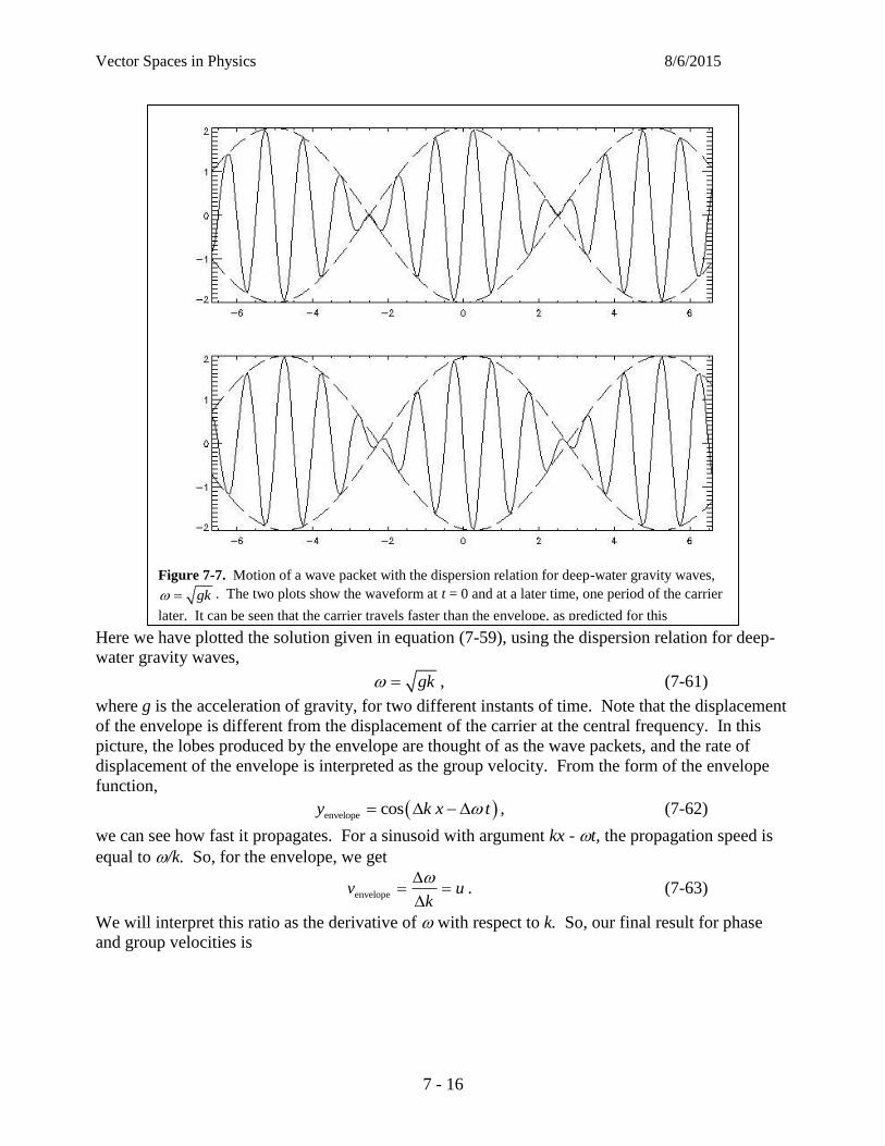
Vector Spaces in Physics 8/6/2015
7 - 16
Here we have plotted the solution given in equation (7-59), using the dispersion relation for deep-
water gravity waves,
gk , (7-61)
where g is the acceleration of gravity, for two different instants of time. Note that the displacement
of the envelope is different from the displacement of the carrier at the central frequency. In this
picture, the lobes produced by the envelope are thought of as the wave packets, and the rate of
displacement of the envelope is interpreted as the group velocity. From the form of the envelope
function,
envelope cosy k x t , (7-62)
we can see how fast it propagates. For a sinusoid with argument kx - t, the propagation speed is
equal to /k. So, for the envelope, we get
envelopev uk
. (7-63)
We will interpret this ratio as the derivative of with respect to k. So, our final result for phase
and group velocities is
Figure 7-7. Motion of a wave packet with the dispersion relation for deep-water gravity waves,
gk . The two plots show the waveform at t = 0 and at a later time, one period of the carrier
later. It can be seen that the carrier travels faster than the envelope, as predicted for this
dispersion relation.
Vector Spaces in Physics 8/6/2015
7 - 17
dispersion relation
phase velocity
group velocity
k
vk
du
dk
(7-64)
Example. For deep-water gravity waves such as storm waves propagating across the pacific
ocean, the velocity of sinusoidal waves is given by
g
vk
. (7-65)
Find the dispersion relation k , and calculate the group velocity u. For waves of wavelength
200 m, calculate the phase and group velocities.
Solution. From the definitions of and k we know that
vT k
.
Solving for omega and using equation 7-65 gives
the dispersion relation
kv
gk
k
kg
.
The group velocity is obtained by taking a derivative:
1
2
d d gu kg
dk dk k
.
Note that the group velocity is exactly equal to half of the phase velocity.
For a wavelength of =200 m, the wave number is
-12 2
0.0314 m200 m
k
.
The phase and group velocities are then
2
-1
9.8 m/s 17.7 m/s ( 35 mph)
0.031415 m
1u= 8.83 m/s
2
gv
k
v
.
[Just in case you ever need it, the general expression for the velocity of gravity waves in water of
depth h is
shallow water
deep watertanh
ghg
v kh gkk
,
reducing correctly to the limiting forms for deep and shallow water given here and in section C
above.]

Vector Spaces in Physics 8/6/2015
7 - 18
Problems
Problem 7-1. The derivative as a limit. To illustrate the derivative as the limit of a rate of
change, consider the function 2
2
1)( attf .
(a) Use the standard rules for taking derivatives (learned in your calculus course) to calculate dt
df.
(b) Now use the definition
t
tfttfLim
dt
df
t
)()(
0
to calculate dt
df. You will need to make an approximation which is appropriate when t is small.
Problem 7-2. Calculation of partial derivatives. In the functions below, x, y, z, and t are to be
considered as variables, and other letters represent constants.
(a) 22axy
x
(b) 22axyy
(c) 2
2
2
2axyx
(d) 2
2
2
2axyy
(e) 22
2axyyx
(f) )sin( tkxAx
(g) )sin( tkxAt
(h) )sin(2
2
tkxAx
(i)
2
2
2exp
d
czB
z
Problem 7-3. Solution to the wave equation. Show by direct substitution that the following
functions satisfy the wave equation,
),(1
),(2
2
22
2
txftv
txfx
.

Vector Spaces in Physics 8/6/2015
7 - 19
You should assume that the relation k
v
holds.
(a) vtxkAtxf cos),(
(b) tkxCtxf cossin),(
Problem 7-4. Derivation of the wave equation for sound. Waves traveling along a tube of gas
can be pictured as shown in the diagram. The small rectangle shows an element of gas, which is
considered to be at position x in the absence of any wave motion. As a wave passes, the
element of gas is displaced by an amount y(x,t), which depends on time and on the position x. The
motion of the element of gas is determined by the pressure on either side, as shown in the lower
part of the diagram.
(a) There will be no net force on the element of gas as long as the pressure is the same on both
sides. However, if there is a variation of pressure with position, there will be a net force F on the
element of gas, of width x , where the force is positive on the left-hand side of the gas element
and negative on the right-hand side, and follows the general relation PAF . The force will thus
be
side hand-righton forceside hand-lefton force F .
Show that this force is given by
xx
PAF
.
Figure p7.4. Forces on an element of gas in an "organ pipe," leading to the wave motion in the
gas.

Vector Spaces in Physics 8/6/2015
7 - 20
(b) We will assume that the pressure in the gas varies by only a small amount from p0, the
ambient background pressure (''atmospheric pressure''):
),(0 txppP .
The variation of p(x,t) with position is in turn related to the displacement of the gas, through the
change in the volume V of the element of gas. A uniform displacement of the gas such that every
part of the gas moves by the same amount does not change the volume of a gas element. However,
if y is a function of x, there is a change in volume. We can use the adiabatic gas law,
constantPV , to relate the small pressure variation p to the corresponding change in volume of
the element of gas:
),(0
0 txpVV
pdP .
Here p0 and V0 are the pressure and volume of the element of gas in the absence of a wave, and is
a constant related to the number of degrees of freedom of the gas molecules (air = 5/3). In this
case, the change in the volume of the element of gas is )(xyxxyAV . Show that this
relation and the relation from the adiabatic gas law lead to the partial-derivative expression
x
ypp
0 .
(c) Now combine the results for parts (a) and (b) and use Newton's 2nd law to find the wave
equation for the displacement y(x,t). Show that the wave velocity v can be given in terms of the
ambient pressure p0 and the gas density =m/V0 by
0pv .
Problem 7-5. Wave speed in telephone wires. Suppose someone wants to send telegraph signals
across the country using the transmission of transverse wave pulses along the wires, rather than
electrical signals. Make a reasonable estimate of the maximum tension in the wires and of their
mass density, and calculate the wave velocity. Assume that the waves run along the wires between
telephone poles, and that they pass right by each telephone pole without reflection. How long
would it take for such a signal to propagate from New York to San Francisco (about 5000 km)?
Problem 7-6. Energy density in a string. The expressions derived in the text for kinetic and
potential energy density are 2
2
2
1KE per unit length =
2
1PE per unit length = -
2
y
t
yT y
x
(7-41)
It is a bit surprising that derivatives with respect to time and position enter in such a different way,
considering how symmetrical their role is in the wave equation. You can fix this up.
The total potential energy over the interval A < x < B is obtained by integrating the energy
density given above: 2
2
1PE between A and B = -
2
x B
x A
yT y dx
x
Vector Spaces in Physics 8/6/2015
7 - 21
Do an integration by parts with respect to x, and show that an equally good expression for the
potential energy density is 2
1PE per unit length =
2
yT
x
You must explain why this is reasonable. Be careful about the evaluation at the endpoints that is
involved in integrating by parts.
Problem 7-7. Phase and group velocity for the deBroglie wave. In 1923 Louis deBroglie
advanced the idea that a free particle of mass m could be described by a wave function, of the form
tkxi
Etpxi
deB
Ae
Aetx
),(
where is Planck's constant, and we will take the non-relativistic forms for the momentum and
energy of the particle,
.2
1
,
2
part
part
mvE
mvp
,
where vpart is the particle's velocity.
(a) Find expressions for k and in terms of the particle velocity vpart.
(b) Show that the dispersion relation for this wave is
.2
)( 2km
k
(c) Calculate the phase velocity and the group velocity for these waves and show how each one
relates to the particle velocity vpart.
(d) It is generally argued that the group velocity is the velocity with which the waves carry energy.
Do your answers to (c) support this argument?
Problem 7-8. Phase and group velocity for the deBroglie wave of a relativistic particle. In
1923 Louis deBroglie advanced the idea that a free particle of mass m could be described by a wave
function, of the form
( , )
p xi
deB
Et pxi
i t kx
x t Ae
Ae
Ae
where is Planck's constant. Note that the phase of the particle, p x Et px
is a relativistic
invariant. We will take the relativistic forms for the momentum and energy of the particle,

Vector Spaces in Physics 8/6/2015
7 - 22
2
2
,
.
E mc
p mc
,
where 2
1
1
, , and
v
c , with v the particle velocity.
(a) Find expressions for k and in terms of , and .
(b) Show that the dispersion relation for this wave is 2
22 2 2( )
mck k
.
(c) Calculate the phase velocity k
and the group velocity
d
dk
for these waves. (It will be
easiest to work with the results of part (a).) The result, in terms of , is very simple and
surprising.
(d) Particles are not supposed to go faster than the speed of light. What do your results of part (c)
say about this?

Vector Spaces in Physics 8/6/2015
8 - 1
Chapter 8. Standing Waves on a String
The superposition principle for solutions of the wave equation guarantees that a sum of waves,
each satisfying the wave equation, also represents a valid solution. In the next section we start with
a superposition of waves going in both directions and adjust the superposition to satisfy certain
requirements of the wave's surroundings.
A. Boundary conditions and initial conditions.
The wave equation results from requiring that a small segment of the string obey Newton's
second law. This is not sufficient to completely specify the behavior of a given string. In general,
we will find it necessary to specify initial conditions, given at a particular time, and boundary
conditions, given at particular places on the string. These conditions determine which of the
manifold of possible motions of the string actually takes place.
The wave equation is a partial differential equation, and is second order in derivatives with
respect to time, and second order in derivatives with respect to position. In general, a second-order
differential equation requires two side conditions to completely determine the solution. For
instance, the motion of a body moving in the vertical direction in the Earth's gravitational field is
not determined until two conditions, such as the initial position and initial velocity, are specified. It
is possible to vary the conditions - for instance, the velocity specified at two different times can
replace position and velocity specified at t = 0.
In the case of the wave equation, to determine the time dependence two conditions must be given,
at a specified time and at all positions on the string. For instance, for a plucked guitar string, the
initial conditions could be that initially the string has zero velocity at all points, and is displaced in
a triangle waveform, with the maximum displacement at the point where it is plucked. Two
additional conditions, the boundary conditions, are required to determine the spatial dependence of
the solution. Each condition specifies something about the displacement of the string, at one
particular point and for all time. For instance, for the guitar string, the displacement of the two
endpoints of the string is required to be zero for all time.
String fixed at a boundary.
A very important type of boundary condition for waves on a string is imposed by fixing one point
on the string. This is usually a point of support for the string, where the tension is applied.
Imagine a traveling-wave pulse like that shown in figure 8-1, traveling from left to right and
approaching a point of attachment of the string, where it cannot move up and down as the wave
passes. The shape of this pulse obviously has to change as it passes over this fixed point,. But the
wave equation says that this pulse will propagate forever, without changing its direction or shape.
How can we get out of this impasse?
The answer is shown in figure 8-1. Here the string occupies the x < 0 part of space, and is
attached to a wall at x = 0, imposing the boundary condition
( 0, ) 0y x t (8.1)
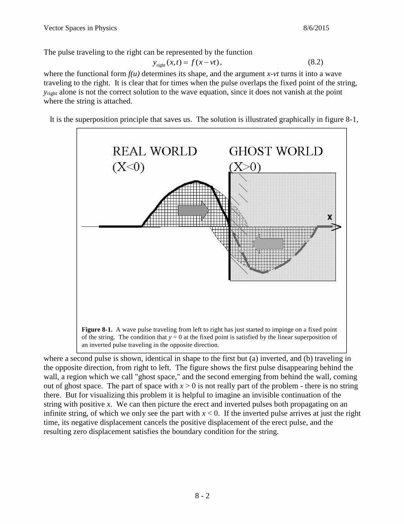
Vector Spaces in Physics 8/6/2015
8 - 2
The pulse traveling to the right can be represented by the function
right ( , ) ( )y x t f x vt , (8.2)
where the functional form f(u) determines its shape, and the argument x-vt turns it into a wave
traveling to the right. It is clear that for times when the pulse overlaps the fixed point of the string,
yright alone is not the correct solution to the wave equation, since it does not vanish at the point
where the string is attached.
It is the superposition principle that saves us. The solution is illustrated graphically in figure 8-1,
where a second pulse is shown, identical in shape to the first but (a) inverted, and (b) traveling in
the opposite direction, from right to left. The figure shows the first pulse disappearing behind the
wall, a region which we call "ghost space," and the second emerging from behind the wall, coming
out of ghost space. The part of space with x > 0 is not really part of the problem - there is no string
there. But for visualizing this problem it is helpful to imagine an invisible continuation of the
string with positive x. We can then picture the erect and inverted pulses both propagating on an
infinite string, of which we only see the part with x < 0. If the inverted pulse arrives at just the right
time, its negative displacement cancels the positive displacement of the erect pulse, and the
resulting zero displacement satisfies the boundary condition for the string.
Figure 8-1. A wave pulse traveling from left to right has just started to impinge on a fixed point
of the string. The condition that y = 0 at the fixed point is satisfied by the linear superposition of
an inverted pulse traveling in the opposite direction.

Vector Spaces in Physics 8/6/2015
8 - 3
How do we write this solution mathematically? If right ( )y f x vt represents the shape f(u),
right side up and traveling to the right, with velocity v, then left ( )y f x vt represents the same
shape f(u), inverted and traveling with velocity -v, to the left. So, a possible solution to the wave
equation which satisfies the boundary condition at the fixed end is
right left( , )
( ) ( )
y x t y y
f x vt f x vt
, (8.3)
Here is how you convince yourself that this is the solution we want. Suppose that the pulse shape
f(u) has its peak at u = 0, and vanishes except when u is fairly close to zero. Now consider the
solution y(x,t) given above, for large negative times. Each term is zero except when its particular
argument is near zero. So, the first pulse will be centered at a large negative x, in the "real world"
part of the string, and the second pulse will be centered at large positive x, out of sight in the "ghost
world." Thus, the initial conditions for this solution are that, at some large negative time, there is a
pulse of shape f(u), with transverse velocity such that it travels to the right. Next, consider the
solution for large positive times. Now yright peaks at positive x, out of sight in the "ghost world,"
and yleft peaks at negative x, where we can see it. Finally, check to see that the boundary condition
is satisfied:
Figure 8-2. A boundary between two parts of a string with different wave propagation velocities.
Shown are a wave incident from the left, a transmitted wave propagating to the right, and a
reflected wave propagating to the left.

Vector Spaces in Physics 8/6/2015
8 - 4
right left( 0, ) ( 0, ) ( 0, )
( ) ( )
0
y x t y x t y x t
f vt f vt
, (8.4)
The form of the solution is such that at the point x = 0 the displacement vanishes, for all times.
Boundary between two different strings.
We can phrase a more general boundary condition for a string. Suppose that at x = 0 the string
attaches, not to a wall, but to another string with a different mass density. There will in general be
both a reflected pulse and a pulse transmitted across the boundary. The situation is shown in figure
8-2, with incident and reflected waves in region 1 and a transmitted wave in region 2. The mass
density in region 1 is 1, corresponding to wave speed 1
1
Tv
, and in region 2 a mass density of
2 gives 2
2
Tv
. The waves in region 1 must travel at the same speed, in order that the
emerging wave comes out at the same rate that the disappearing wave comes in. Thus in region 1
we will use the function
1 1 1( , ) 0 (region 1)y x t Af x v t Bf x v t x (8.5)
In region 2, the wave must have a different shape; if it travels slower, it must appear shorter when
plotted as a function of position, so that it emerges into region 2 during the precise time interval
when the incoming wave of region 1 disappears. This means that we have to use the function
1
2 2 2
2
( , ) ( ) 0 (region 2)v
y x t Cg x v t Cf x v t xv
(8.6)
This is an awkward-looking function; however, notice that
(a) the functions used for y1 are solutions of the wave equation traveling with speed v1 and
the function used for y2 is a solution of the wave equation traveling with speed v2.
(b) If we set x to zero, all of the functions used have a common factor of f(-v1t).
We will now use these properties to match boundary conditions at x = 0.
The boundary conditions at a boundary between two regions of the string with different
propagation speeds are:
1 2
1 2
0 0
( 0, ) ( 0, ) continuity of the displacement
y ycontinuity of the slope
x xx x
y x t y x t
Boundary Conditions for Waves on a String
(8.7)
The reason for having the displacement the same on each side of the boundary is obvious - the two
strings are attached to each other. The reason for the slopes being equal can be understood by
considering the forces acting at the point where the two strings join (x = 0). The situation is similar
to that shown in figure 7-3; the magnitude of the force exerted from the right-hand side and from
the left-hand side is the same, but if the slopes are not the same, there will be a net transverse force.
For a finite difference in slope, there would be a finite force acting on an infinitesimal element of
string, giving it an infinite transverse acceleration. This is not possible; if there were a finite
Vector Spaces in Physics 8/6/2015
8 - 5
transverse force, the string would just move quickly up or down until the slopes equalized. Thus
the slope may be assumed to be continuous across the boundary.
Applying the boundary conditions gives
1 2
1 1 1
( 0, ) ( 0, )
( ) ( ) ( )
y x t y x t
Af v t Bf v t Cf v t
A B C
(8.8)
and
1 2
00
1
1 1 1
2
1
2
y y
x x
( )
xx
vAf v t Bf v t Cf v t
v
vA B C
v
(8.9)
We can add equation 8-8 to equation 8-9, eliminating B, and solve for the "transmission
coefficient" T C/A. Similarly one can eliminate C and find the "reflection coefficient" R B/A.
The results are:
2
2 1
2 1
2 1
2vCT
A v v
v vBR
A v v
(8.10)
Example. Consider the limiting case where the second string, in region 2 with x > 0, has a much
higher mass density than the string in region 1. Show that this leads to the result that we found
above for a string fixed at one end.
Solution. In the case where 2 1 , the relation T
v
tells us that 2 1v v . In this limit, the
transmission and reflection coefficients become
2
1 2
1 2
1 2
20
1
vT
v v
v vR
v v
(8.11)
That is, there is no transmitted wave, and the reflected wave is inverted and of the same magnitude
as the incident wave. This is the result that we found above for simple pulse reflection from a fixed
end.

Vector Spaces in Physics 8/6/2015
8 - 6
B. Standing waves on a
string.
Now we are ready to take on one of
the famous problems in physics - the
vibrations of a string held fixed at
both ends. The most familiar
application of this theory is to the
stringed musical instruments, but the
mathematical patterns displayed here
are applied very widely in physics.
the problem is stated pictorially in
figure 8-3.
The string will be described by a
wave function ,y x t which must
satisfy the wave equation for all x in
the interval (0,L), and which must
obey the boundary conditions
0, 0
, 0
y x t
y x L t
, (8.12)
There are many such functions. The irregularly wiggling profile shown in figure 8-3 is a possible
"snapshot" of the position of the string at one instant of time - if you held the string in that position
and let it go, it would certainly do something! We are going to look however for certain special
solutions, called standing waves, of the form
, cosy x t X x t . (8.13)
This represents a wave which always has the same shape, determined by the function X(x) of
position only, with its time variation restricted to a sinusoidal modulation of this shape. Solutions
like this where everything varies together sinusoidally with time are sometimes referred to as
"normal modes." They are a sort of continuous version of the normal modes for vibrating and
oscillating systems which we discussed in Chapter 4.
Now we substitute this form into the wave equation:
2 2
2 2 2
22
2 2
2 22
2 2
cos cos1
1cos cos
X x t X x t
x v t
d Xt X t
dx v
d XX k X
dx v
. (8.14)
The partial differential equation has turned into an ordinary differential equation, thanks to writing
y(x,t) as a product of a function of x and a function of t. [You may recognize this from a course on
differential equations as the method of separation of variables. It makes it easy to find a variety of
solutions to the wave equation. It is a trickier matter to convince yourself that you find all the
solutions this way.]
Figure 8-3. A string stretched between two fixed points, at x = 0 and
x = L.

Vector Spaces in Physics 8/6/2015
8 - 7
Equation 8-14 is fairly easy to solve:
sin cosX x A kx B kx . (8.15)
giving
, cos sin cos cosy x t X x t A kx B kx t . (8.16)
How can we make this solution satisfy the boundary conditions, equation 8-12, for all values of t?
The only way to make the function vanish at x = 0 is to take 0B . The solution is now
, sin cosy x t A kx t . (8.17)
To make this vanish at x = L requires the sine to vanish there:
sin 0
, n = 1, 2, 3, . . . .n
kL
nk k
L
. (8.18)
Note that choosing fixed values of k also chooses corresponding values of , via the relation
kv . This is where the resonant frequencies of the string are determined!
Thus, the solutions of the type sin cosA kx t satisfying the boundary conditions are
n
, sin cos
k
12 , n = 1, 2, 3, . . . .
2
n n n n
n
n
n
y x t k x t
nL
Ln
vn
L
vf n
L
. (8.19)
The functions n are the normal modes for the vibrating string, representing the special shapes of
the string which oscillate in time without changing their form. They are described in figure 8-4,
where the envelope function sin nk x is plotted for increasing values of n.

Vector Spaces in Physics 8/6/2015
8 - 8
.
Problems
Problem 8-1. Reflection and transmission coefficients for sinusoidal waves. Consider the
problem discussed in the text of a sinusoidal wave propagating down a string from left to right, as
shown in figure 8.2. The string changes its mass density at x = 0, from a value 1 to a value 2, with
a corresponding change in propagation velocity, from v1 to v2. There is a reflected wave which
travels back along the left-hand string, in the opposite direction but with the same velocity, and a
transmitted wave, which continues to the right with velocity v2. Take the waves on the string to be
sinusoidal traveling waves, given by
1 1 1
2 2
( , ) cos( ) cos( ), 0
( , ) cos( ), 0
y x t A k x t B k x t x
y x t C k x t x
Note that the wave number vk / is different in the two parts of the string, but that the
frequency is the same.
Use the conditions of continuity of the displacement and its derivative (eqn (8.7)) to derive
the expressions for the reflection and transmission coefficients T=C/A and R=B/A in terms of v1
and v2, as given in equation (8.10). [The relations in equation (8-10) were derived for the more
Figure 8-4. The normal modes of a vibrating string.

Vector Spaces in Physics 8/6/2015
8 - 9
general case of an arbitrary traveling wave. You are checking them for the special case of a
sinusoidal wave.]
Problem 8-2. In section A above we considered the case of a wave incident on the boundary
between strings of different mass densities, in the limit where the second string was much heavier
than the first ( 2 1 ). Carry out the same sort of analysis of the limiting case where the second
string is much lighter ( 2 1 ). Describe what the reflection of a pulse traveling down the string
would look like in this limiting case.

Vector Spaces in Physics 8/6/2015
9 - 1
Chapter 9. Fourier Series
A. The Fourier Sine Series
The general solution. In Chapter 8 we found solutions to the wave equation for a string fixed at
both ends, of length L, and with wave velocity v,
n
, sin cos
k
12 , n = 1, 2, 3, . . . .
2
n n n n
n
n
n
y x t A k x t
nL
Ln
vn
L
vf n
L
. (9-1)
We are now going to proceed to describe an arbitrary motion of the string with both ends fixed in
terms of a linear superposition of normal modes:
1
general solution, string, sin cos
fixed at both endsn n
n
n xy x t A t
L
, (9-2)
where n
n v
L
and the coefficients An are to be determined. Here are some things to be noted:
(1) We are assuming for the moment that this equation is true - that is, in the limit where
we include an infinite number of terms, that the infinite series is an arbitrarily good approximation
to the solution ,y x t .
(2) Each term in the series is separately a solution to the wave equation satisfying the
boundary conditions, and so the series sum itself is such a solution.
(3) This series is sort of like an expansion of a vector in terms of a set of basis vectors. In
this picture the coefficients An are the coordinates of the function ,y x t .
(4) We still have to specify initial conditions and find a method to ensure that they are
satisfied. This is the next order of business.
Initial conditions.
The solution above satisfies the boundary conditions appropriate to the problem,
0, , 0.y t y L t But no initial conditions have been proposed. A complete set of initial
conditions would consist of specifying the displacement of the string at some initial time, say t = 0,
and the velocity of the string at the same time. These conditions might look as follows:
Vector Spaces in Physics 8/6/2015
9 - 2
0
,0
( )t
y x f x
yg x
t
. (9-3)
It might be noticed by the astute observer that if we take the partial derivative of equation (9-2)
with respect to time and set t = 0, it vanishes identically. (Each term would have a factor of sin nt
, which vanishes at t = 0.) This means that we have already built into this solution the condition
that the string is not moving at t = 0; or, in terms of the initial conditions just stated,
0g x . (9-4).
This is a limitation; if we wanted equation (9-2) to be completely general, we would have to add
another set of terms multiplied by factors of cosnt . This makes things quite a bit more
complicated and does not add very much to the understanding of Fourier series; we will just live
with the limitation to wave motions where the string is stationary at t = 0.
This leaves us with the condition on the displacement at t = 0, which takes
on the form
1
,0 sinn
n
n xy x f x A
L
. (9-5).
The series
1
sin Fourier sine seriesn
n
n xf x A
L
. (9-6).
is a very famous equation in mathematics, representing the statement that any function of x defined
on the interval [0,L] and vanishing at the ends of the interval can be represented as a linear
superposition of the sine waves vanishing at the ends of the interval. We will now spend some time
seeing how this works.
Orthogonality.
If the functions sinn x
L
are to play the role of basis vectors in this process, it would be nice if
they were orthogonal. To define orthogonality we need to define an inner product. For functions
defined on the interval [0,L], a useful definition of an inner product is the following:
0
, inner product
L
x
u v u x v x dx
(9-7)
Orthogonality of two functions u x and v x means that , 0u v . For the functions sinn x
L
,
if this inner product is evaluated, the result is
0
sin ,sin sin sin2
L
nm
x
n x m x n x m x Ldx
L L L L
(9-8)
Vector Spaces in Physics 8/6/2015
9 - 3
where nm is the Kronecker delta symbol. (The proof of this fact is left to the problems.) So, the
functions sinn x
L
almost constitute an orthonormal basis for the space of functions we are
considering. They could be properly normalized by multiplying each one by a factor of 2
L. This
is not usually done, just to keep the equations simpler.
Now we need a way to find the coefficients , n = 1, 2, 3, ...nA . If we remember the method for
determining the coordinates of vectors, it is very easy:
0
2,sin
inversion of Fourier series2
sin
m
L
x
m xA f x
L L
m xf x dx
L L
(9-9)
This important relation can be verified as follows:
1
10 0
1 0
1
sin
2 2sin sin sin
2sin sin
2
2
n
n
L L
n
nx x
L
n
n x
n nm
n
m
n xf x A
L
m x n x m xf x dx A dx
L L L L L
n x m xA dx
L L L
LA
L
A
(9-10)
Here we have of course used the orthogonality relation, equation 9-8. Thus for any given initial
condition f x we can calculate the coefficients An, and use equation 9-2 to calculate the position
at any time, to any desired accuracy.
Completeness.
The functions sinn x
L
are not only orthogonal. They are a “complete” representation of
functions of x over the interval 0 ≤ x ≤ L, meaning that such functions can be represented arbitrarily
well by a linear combination of these sine functions. A somewhat more precise statement of this
completeness condition is that given by Dirichlet:
For any function which is piecewise continuous over the interval [0,L], the Fourier series
1
sinn
n
n xA
L
(9-11)
converges to f(x) at every point. At points of discontinuity, the series converges to the
average of f(x-) and f(x+).

Vector Spaces in Physics 8/6/2015
9 - 4
So we have found one of the most important expansions of a function as a series of orthogonal
functions:
1
m
0
sin
with
2A sin
n
n
L
x
n xf x A
L
m xf x dx
L L
The Fourier Sine Series
0 < x <L
(9-12)
Example. Calculate the Fourier coefficients of a Fourier sine series for the symmetrical triangle
wave, shown in figure 9-1.
Solution. The function f(x) can be written
Figure9-1. Initial conditions for the triangle wave, initially displaced by an amount h at the center.

Vector Spaces in Physics 8/6/2015
9 - 5
2, 0
2
2,
2
h Lx x
Lf x
h LL x x L
L
(9-13)
and then the coefficients An can be evaluated:
0
/ 2
0 / 2
/ 2
2 2
0 / 2 / 2
2sin
2 2 2 2sin sin
4 4 4sin sin sin
L
m
x
L L
x x L
L L L
x x L x L
m xA f x dx
L L
h m x h m xx dx L x dx
L L L L L L
h m x h m x h m xx dx x dx dx
L L L LL L
(9-14)
There are various ways to do tiresome integrals like these. My preferred method is to change to
dimensionless variables, then do the integrals by parts. So I will change to the variable m x
uL
,
giving 2 / 2
2
0 / 2 / 2
/ 2/ 2
2 2 0 / 2 / 2
0 / 2
/
2 2 0
4 4sin sin sin
4 4cos cos cos sin cos
42 cos cos sin
2 2
m m m
m
u u m u m
m mm m m
u m u m
u u m
m
u
h L h LA u u du u u du udu
m L mL
h hu u u u u du u du u
mm
h m mm m u
m
2
/ 2
2 2
4sin cos cos
2
8sin
2
m
u m
h mu m
m
h m
m
(9-15)
This finally simplified rather well. We could leave the result as it is, but another change shows the
pattern to the values of the coefficients better. We observe that sin2
m vanishes for m even; and
for m odd,
1
2sin 1 (m odd)2
mm
(9-16)
Thus the result is
1
22 2
0, even
81 , odd
mm
m
A hm
m
(9-17)
The corresponding series for f(x) is
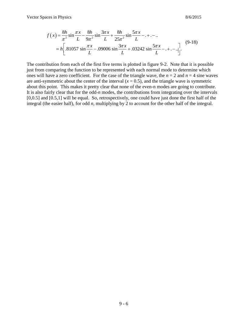
Vector Spaces in Physics 8/6/2015
9 - 6
2 2 2
8 8 3 8 5sin sin sin . . ..
9 25
3 5.81057 sin .09006 sin .03242 sin . . .. .
h x h x h xf x
L L L
x x xh
L L L
(9-18)
The contribution from each of the first five terms is plotted in figure 9-2. Note that it is possible
just from comparing the function to be represented with each normal mode to determine which
ones will have a zero coefficient. For the case of the triangle wave, the n = 2 and n = 4 sine waves
are anti-symmetric about the center of the interval (x = 0.5), and the triangle wave is symmetric
about this point. This makes it pretty clear that none of the even-n modes are going to contribute.
It is also fairly clear that for the odd-n modes, the contributions from integrating over the intervals
[0,0.5] and [0.5,1] will be equal. So, retrospectively, one could have just done the first half of the
integral (the easier half), for odd n, multiplying by 2 to account for the other half of the integral.

Vector Spaces in Physics 8/6/2015
9 - 7
B. The Fourier sine-cosine series
The preceding discussion was based on the analysis of a string fixed at x = 0 and x = L, and it
made sense to expand the initial displacement in terms only of functions obeying the same
restrictions. However, there is a more general form of the Fourier series which gives a complete
representation of all functions over the interval [-L,L], independent of their symmetry and with no
requirement that they vanish at any particular points. This is the series
Figure 9-2. The Fourier series for the triangle wave. There is a graph for each value of sinn x
L
(dash-dot line), the
nth term in the expansion (dashed line), and the nth partial sum (dark line).
Vector Spaces in Physics 8/6/2015
9 - 8
0
1
1sin cos
2n n
n
n x n xf x B A B
L L
The Fourier Sine - Cosine Series
-L < x < L (9-19)
The inner product for this interval is now
,
L
L
u v u x v x dx
(9-20)
and the inversion formulae for this series are
1sin
1cos
L
m
x L
L
m
x L
m xA f x dx
L L
m xB f x dx
L L
(9-21)
Odd and even functions.
In the inversion formulae, equation (9-21) above, the range of integration, from –L to L, is
symmetric about the point x = 0. The functions sinm x
L
and cos
m x
L
have definite symmetry
about x = 0, and this can make the job of carrying out the integrations in equation (9-21) easier.
Functions are said to be even or odd about x=0 if they satisfy one of the following conditions:
( ) ( ) even function
( ) ( ) odd function
g x g x
h x h x
(9-22)
Example. Here some functions of x. Which ones are even or odd?
2
3
( ) sin
( )
( )
( ) x
a x
b x
c x
d e
Solution.
(a) From the properties of the sine function, sin( ) sin( )x x
So, this is an odd function.
(b) Using simple algebra,
2 2 2
2
1x x
x
This is therefore an even function.
(c) Similarly,
3 3 3
3
1x x
x

Vector Spaces in Physics 8/6/2015
9 - 9
This is therefore an odd function.
(d) Compare
( ) xf x e
and
( ) xf x e .
This function is always positive, so it cannot be odd. And, while f x is greater than 1, f x
is less than 1, and so f x cannot be even. So, this function is neither even nor odd.
There are some general conclusions which can be drawn about odd and even functions. It is easy
to see that
The product of two even functions is an even function.
The product of two odd functions is an even function.
The product of an even function and an odd function is an odd function.
Some important properties of their integrals can also be demonstrated. Let g x
be an even function of x, and h(x) an odd function of x. Then it is easy to see that
0
2
L L
L
g x dx g x dx
(9-23)
and
0
L
L
h x dx
(9-24)
Periodic functions in time.
The Fourier expansion of functions of time plays a very important role in the analysis of signals, in
electrical engineering and other fields. A periodic function of time with period T can be expanded
as follows:
0
1
( ) sin cos2
n n n n
n
Bf t A t B t
(9-25)
where
2
n
n
T
(9-26).
The inversion formula is
/ 2
/ 2
/ 2
/ 2
2sin ,
2cos .
T
n n
T
T
n n
T
A f t t dtT
B f t t dtT
(9-27)
Example. Calculate the coefficients of the Fourier series for the square wave shown in
figure (9-3), consisting of a pulse waveform with value 1 from t = -T/4 to t = T/4, and zero
over the rest of the interval [-T/2, T/2]. (The value of the function for all other values of t is
determined by its periodicity.)
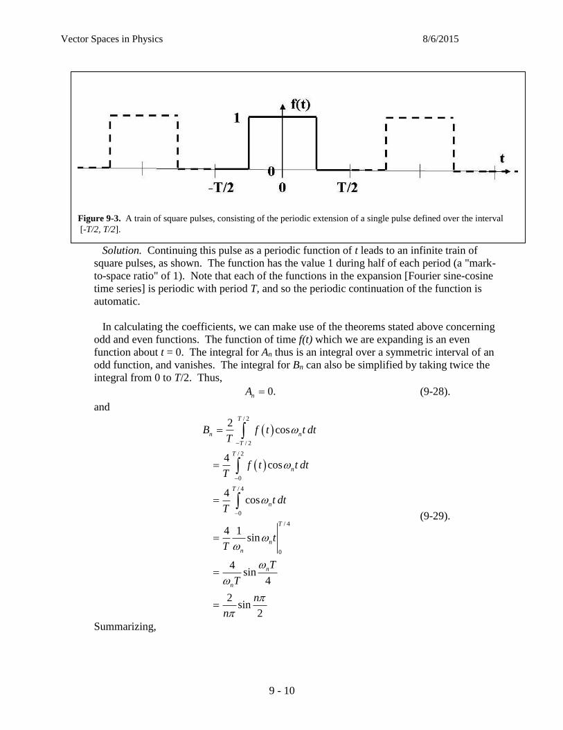
Vector Spaces in Physics 8/6/2015
9 - 10
Solution. Continuing this pulse as a periodic function of t leads to an infinite train of
square pulses, as shown. The function has the value 1 during half of each period (a "mark-
to-space ratio" of 1). Note that each of the functions in the expansion [Fourier sine-cosine
time series] is periodic with period T, and so the periodic continuation of the function is
automatic.
In calculating the coefficients, we can make use of the theorems stated above concerning
odd and even functions. The function of time f(t) which we are expanding is an even
function about t = 0. The integral for An thus is an integral over a symmetric interval of an
odd function, and vanishes. The integral for Bn can also be simplified by taking twice the
integral from 0 to T/2. Thus,
0.nA (9-28).
and
/ 2
/ 2
/ 2
0
/ 4
0
/ 4
0
2cos
4cos
4cos
4 1sin
4sin
4
2sin
2
T
n n
T
T
n
T
n
T
n
n
n
n
B f t t dtT
f t t dtT
t dtT
tT
T
T
n
n
(9-29).
Summarizing,
Figure 9-3. A train of square pulses, consisting of the periodic extension of a single pulse defined over the interval
[-T/2, T/2].
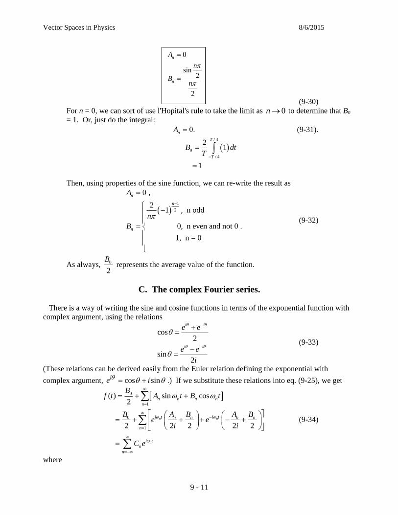
Vector Spaces in Physics 8/6/2015
9 - 11
(9-30)
For n = 0, we can sort of use l'Hopital's rule to take the limit as 0n to determine that Bn
= 1. Or, just do the integral:
0.nA (9-31).
/ 4
0
/ 4
21
1
T
T
B dtT
Then, using properties of the sine function, we can re-write the result as
1
2
0 ,
21 , n odd
0, n even and not 0 .
1, n = 0
n
n
n
A
n
B
(9-32)
As always, 0
2
B represents the average value of the function.
C. The complex Fourier series.
There is a way of writing the sine and cosine functions in terms of the exponential function with
complex argument, using the relations
cos2
sin2
i i
i i
e e
e e
i
(9-33)
(These relations can be derived easily from the Euler relation defining the exponential with
complex argument, cos sinie i .) If we substitute these relations into eq. (9-25), we get
0
1
0
1
( ) sin cos2
2 2 2 2 2n n
n
n n n n
n
i t i tn n n n
n
i t
n
n
Bf t A t B t
B A B A Be e
i i
C e
(9-34)
where
0
sin2
2
n
n
A
n
Bn
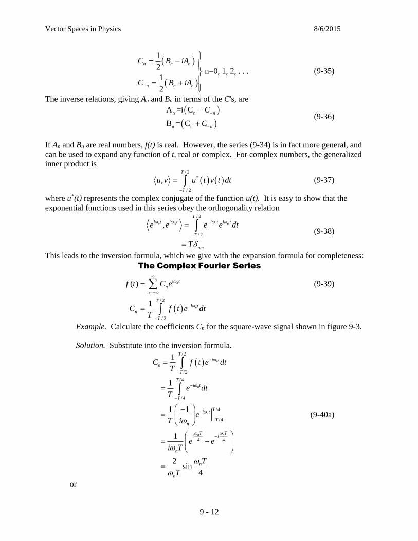
Vector Spaces in Physics 8/6/2015
9 - 12
1
2n=0, 1, 2, . . .
1
2
n n n
n n n
C B iA
C B iA
(9-35)
The inverse relations, giving An and Bn in terms of the C's, are
n n
n n
A =i C
B = C
n
n
C
C
(9-36)
If An and Bn are real numbers, f(t) is real. However, the series (9-34) is in fact more general, and
can be used to expand any function of t, real or complex. For complex numbers, the generalized
inner product is
/ 2
*
/ 2
,
T
T
u v u t v t dt
(9-37)
where u*(t) represents the complex conjugate of the function u(t). It is easy to show that the
exponential functions used in this series obey the orthogonality relation
/ 2
/ 2
,n m n m
T
i t i t i t i t
T
nm
e e e e dt
T
(9-38)
This leads to the inversion formula, which we give with the expansion formula for completeness:
/ 2
/ 2
( )
1
n
n
i t
n
n
T
i t
n
T
f t C e
C f t e dtT
The Complex Fourier Series
(9-39)
Example. Calculate the coefficients Cn for the square-wave signal shown in figure 9-3.
Solution. Substitute into the inversion formula.
/2
/2
/4
/4
/4
/4
4 4
1
1
1 1
1
2sin
4
n
n
n
n n
T
i t
n
T
T
i t
T
Ti t
Tn
T Ti i
n
n
n
C f t e dtT
e dtT
eT i
e ei T
T
T
(9-40a)
or

Vector Spaces in Physics 8/6/2015
9 - 13
( 1)/2
1sin n = . . . -2, -1, 0, 1, 2, . . .
2
1/ 2 0
0 even
11 odd
n
n
n
nC
n
n
n
n
(9-40)
As with the coefficient Bn, the case of n=0 has to be interpreted in terms of the limit as
0n , giving C0 = 1/2, the correct average value for the square-wave function.
Problems
Problem 9-1. Orthogonality of the sine functions. The spatial dependence of the standing-wave
solutions for waves on a string of length L is given by
L
xnxf n
sin)( , n = 1,2,3, . . . .
Prove the orthogonality relation for these functions,
nmmn
Lff
2, ,
where the inner product is defined by
dxxfxfff m
L
x
nmn )()(,0
.
To carry out this integral, substitute in the definition of the sine function in terms of complex
exponentials,
i
ee
L
xn L
xni
L
xni
2sin
[Please do this integral "by hand," not with Mathematica.]
Problem 9-2. Odd and even functions. For each of the following functions, determine whether
it is even, odd, or neither, under reflection about the origin.
(a) xcos
(b) xxsin
(c) x
(d) 432 2 xx
Problem 9-3. Products of odd and even functions. Suppose that f(x) and g(x) are even functions
and h(x) is an odd function - that is,

Vector Spaces in Physics 8/6/2015
9 - 14
.)()(
,)()(
,)()(
xhxh
xgxg
xfxf
Prove the following two properties:
(a) The product of two even functions is an even function; that is, the function u(x) = f(x)*g(x) is
an even function.
(b) The product of an even and an odd function is odd; that is, the function v(x) = f(x)*h(x) is an
odd function.
Problem 9-4. Integral of odd and even functions over a symmetrical range of integration. Prove that, for f(x) an even function about x=0 and h(x) an odd function,
a
a
dxxh 0)(
and
aa
a
dxxfdxxf0
)(2)( .
To carry out this proof, break the integral up into an integral from -a to 0 and another from 0 to a,
and, for the integral over negative values of x, make a change of variable, from x to a new variable
y, with y = -x.
Problem 9-5. Fourier coefficients for a square wave. Calculate the coefficients An in the Fourier
sine series,
1
sin , 0n
n
n xf x A x L
L
for the square-wave function.
Lxx
Lxxf
or0,0
0,1)(
Problem 9-6. Numerical evaluation of the expansion of the square wave. Use Excel to make a
series of graphs, showing the curve obtained from the partial sums of 1, 3, 5, 7, and 9 terms of the
expansion of the square wave discussed in problem 9.5. Each graph should show the n-th term in
the sum, and the n-th partial sum. Take L = 1, so that the x-axis on the plots runs from 0 to 1. (In
case you didn't do problem 9.5, the answer is
1
sin , 0n
n
n xf x A x L
L
4, n odd
0, n evennA n
.)
Here is a suggested layout for a spreadsheet.
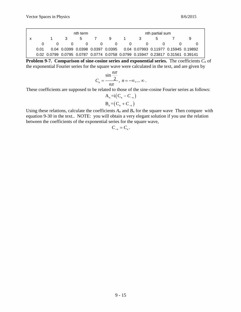
Vector Spaces in Physics 8/6/2015
9 - 15
Problem 9-7. Comparison of sine-cosine series and exponential series. The coefficients Cn of
the exponential Fourier series for the square wave were calculated in the text, and are given by
sin2 , ,... n
n
C nn
.
These coefficients are supposed to be related to those of the sine-cosine Fourier series as follows:
n n
n n
A =i C
B = C
n
n
C
C
Using these relations, calculate the coefficients An and Bn for the square wave Then compare with
equation 9-30 in the text.. NOTE: you will obtain a very elegant solution if you use the relation
between the coefficients of the exponential series for the square wave,
n nC C .
nth term nth partial sum
x 1 3 5 7 9 1 3 5 7 9
0 0 0 0 0 0 0 0 0 0 0
0.01 0.04 0.0399 0.0398 0.0397 0.0395 0.04 0.07993 0.11977 0.15945 0.19892
0.02 0.0799 0.0795 0.0787 0.0774 0.0758 0.0799 0.15947 0.23817 0.31561 0.39141

Vector Spaces in Physics 8/6/2015
10 - 1
Chapter 10. Fourier Transforms and the Dirac Delta Function
A. The Fourier transform.
The Fourier-series expansions which we have discussed are valid for functions either defined over a
finite range ( / 2 / 2T t T , for instance) or extended to all values of time as a periodic function.
This does not cover the important case of a single, isolated pulse. But we can approximate an
isolated pulse by letting the boundaries of the region of the Fourier series recede farther and farther
away towards , as shown in figure 10-1. We will now outline the corresponding mathematical
limiting process. It will transform the Fourier series, a superposition of sinusoidal waves with
discrete frequencies n, into a superposition of a continuous spectrum of frequencies .
As a starting point we rewrite the Fourier series, equation 9-39, as follows:
/ 2
/ 2
( )
1
n
n
i t
n
n
T
i t
n
T
f t C e n
C f t e dtT
(10-1)
The only change we have made is to add, in the upper expression, a factor of n for later use;
1 1n n n is the range of the variable n for each step in the summation. We now imagine
letting T get larger and larger. This means that the frequencies
Figure10-1. Evolution of a periodic train of pulses into a single isolated pulse, as the domain of the Fourier series goes
from [-T/2, T/2] to [-, ].

Vector Spaces in Physics 8/6/2015
10 - 2
2
n
n
T
(10-2)
in the sum get closer and closer together. In the large-n approximation we can replace the integer
variable n by a continuous variable n, so that
n
n
n n
C C n
n
n dn
(10-13)
We thus have
/ 2
/ 2
( )
1
i n t
n
Ti n t
T
f t C n e dn
C n f t e dtT
(10-4)
Next we change variables in the first integral from n to 2 n
nT
:
/ 2
/ 2
( )2
1
i t
T
i t
T
Tf t C e d
C f t e dtT
(10-5)
Now define
2
Tg C
(10-6)
This gives
/ 2
/ 2
1( )
2
1
2
i t
T
i t
T
f t g e d
g f t e dt
(10-7)
Finally, we take the limit T , giving the standard for m for the Fourier transform:
1
( )2
i tf t g e d
Inverse Fourier Transform (10-8)
1
2
i tg f t e dt
Fourier Transform (10-9)
There are a lot of notable things about these relations. First, there is a great symmetry in the roles
of time and frequency; a function is completely specified either by f(t) or by g(). Describing a
function with f(t) is sometimes referred to as working in the "time domain," while using g() is
referred to as working in the "frequency domain." Second, both of these expressions have the form
of an expansion of a function in terms of a set of basis functions. For f(t), the basis functions are

Vector Spaces in Physics 8/6/2015
10 - 3
1
2
i te
; for g(), the complex conjugate of this function,
1
2
i te
, is used. Finally, the
function g() emerges as a measure of the "amount" of frequency which the function f(t)
contains. In many applications, plotting g() gives more information about the function than
plotting f(t) itself.
Example - the Fourier transform of the square pulse. Let us consider the case of an isolated
square pulse of length T, centered at t = 0:
1,
( ) 4 4
0 otherwise
T Tt
f t
(10-10)
This is the same pulse as that shown in figure 9-3, without the periodic extension. It is
straightforward to calculate the Fourier transform g():
/ 4
/ 4
4 4
1
2
1
2
1 1
2
sin4
2 2
4
i t
t
T
i t
t T
T Ti i
g f t e dt
e dt
e ei
T
T
T
(10-11)
Here we have used the relation sin2
i ie e
i
. We have also written the dependence on in the
form sin
sincx
xx
. This well known function peaks at zero and falls off on both sides, oscillating
as it goes, as shown in figure 10-2.
B. The Dirac delta function (x).
The Dirac delta function was introduced by the theoretical physicist P.A.M. Dirac, to describe a
strange mathematical object which is not even a proper mathematical function, but which has many
uses in physics. The Dirac delta function is more properly referred to as a distribution, and Dirac
played a hand in developing the theory of distributions. Here is the definition of (x):
1)(
0,0)(
dxx
xx
(10-12)

Vector Spaces in Physics 8/6/2015
10 - 4
Isn't this a great mathematical joke? This function is zero everywhere! Well, almost everywhere,
except for being undefined at x=0. How can this be of any use? In particular, how can its integral
be anything but zero? As an intellectual aid, let's compare this function with the Kronecker delta
symbol, which (not coincidentally) has the same symbol:
1
,1
,0
3
1
i
ij
ijji
ji
(10-13)
There are some similarities. But the delta function is certainly not equal to 1 at x = 0; for the
integral over all x to be equal to 1, (x) must certainly diverge at x = 0 In fact, all the definitions
that I know of a Dirac delta function involve a limiting procedure, in which (x) goes to infinity.
Here are a couple of them.
The rectangular delta function
Consider the function
Figure10-2. The Fourier transform of a single square pulse. This function is sometimes called the sync function.

Vector Spaces in Physics 8/6/2015
10 - 5
0
1/ x2
( ) lim
0 x2
aa
xa
(10-14)
This function, shown in figure 10-3, is a rectangular
pulse of width a and height h = 1/a. Its area is equal to
( ) 1A f x dx h a
, so it satisfies the integral
requirement for the delta function. And in the limit that
a 0, it vanishes at all points except x = 0. This is one
perfectly valid representation of the Dirac delta
function.
The Gaussian delta function
Another example, which has the advantage of being an
analytic function, is
.
2
22
0
1 1( ) lim
2
x
x e
(10-15)
The function inside the limit is the Gaussian function, 2
221 1
( )2
x
g x e
(10-16)
in a form often used in statistics which is normalized so that
1)(
dxxg , and so that the standard deviation of the
distribution about x=0 is equal to . A graph of the
Gaussian shape was given earlier in this chapter; the width
of the curve at half maximum is about equal to 2. (See
figure 10-4.) It is clear that in the limit as goes to zero
this function is zero everywhere except at x = 0 (where it
diverges, due to the factor 1
), maintaining the
normalization condition all the while.
Properties of the delta function
By making a change of variable one can define the delta function in a more
general way, so that the special point where it diverges is x = a (rather
than x=0):
x
)
g(x)
Figure 10-4. The Gaussian function,
becoming a delta function in the limit
0 .
x
a 1/a
f(x)
Figure 10-3. Rectangular function,
becoming a delta function in the limit a 0.

Vector Spaces in Physics 8/6/2015
10 - 6
1)(
,0)(
dxax
axax
(10-17)
Two useful properties of the delta function are given below:
( ) ( ) ( )f x x a dx f a
, (10-18)
( ) '( ) '( )f x x a dx f a
, (10-19)
Here the prime indicates the first derivative.
The property given in equation (10-18) is fairly easy to understand; while carrying out the integral,
the argument vanishes except very near to x=a; so, it makes sense to replace f(a) by the constant
value f(a) and take it out of the integral. The second property, Eqn. (10-19), can be demonstrated
using integration by parts. The proof will be left to the problems.
C. Application of the Dirac delta function to Fourier transforms
Another form of the Dirac delta function, given either in k-space or in -space, is the following:
0
0
( )
0
( )
0
1( )
2
1( )
2
i k k x
i x
e dx k k
e dx
. (10-20)
We will not prove this fact, but just make an argument for its plausibility. Look at the integral (10-
20), for the case when k = k0. The exponential factor is just equal to 1 in that case, and it is
clear that the integral diverges. On the other hand, if k is not equal to k0, it is plausible that the
oscillating nature of the argument makes the integral vanish. If we accept these properties, we can
interpret the Fourier transform as an expansion of a function in terms of an orthonormal basis, just
as the Fourier series is an expansion in terms of a series of orthogonal functions. Here is the picture.
Basis states
The functions
tiee
2
1)(ˆ . (10-21)
constitute a complete orthonormal basis for the space of ''smooth'' functions on the interval
t . We are not going to prove completeness; as with the Fourier series, the fact that the
expansion approximates a function well is usually accepted as sufficient by physicists. The
orthonormality is defined using the following definition of an inner product of two (possibly
complex) functions u(t) and v(t):
vdtuvu
*, . (10-22)
where u* represents the complex conjugate of the function u(t). Now the inner product of two basis
states is

Vector Spaces in Physics 8/6/2015
10 - 7
)(
2
1
ˆˆˆ,ˆ*
dtee
dteeee
titi (10-23)
(The proof of the last line in the equation above is beyond the scope of these notes - sorry.) This is
the equivalent of the orthogonality relation for sine waves, equation (9-8), and shows how the Dirac
delta function plays the same role for the Fourier transform that the Kronecker delta function plays
for the Fourier series expansion.
We now use this property of the basis states to derive the Fourier inversion integral. Suppose that
we can expand an arbitrary function of t in terms of the exponential basis states:
.
degtf ti)(2
1)( (10-24)
Here represents a sort of weighting function, still to be determined, to include just the right
amount of each frequency to correctly reproduce the function f(t). This is a continuous analog of
the representation of a vector A
in terms of its components,
.
jjeAA ˆ
(10-25)
The components Ak are obtained by taking the inner product of the k-th basis vector with A
:
.
AeA kk
ˆ (10-26)
If the analogy holds true, we would expect the weighting function (the ''coordinate'') to be
determined by
dttfe
dttfe
tfeg
ti
ti
ti
)(2
1
)(2
1
)(,2
1
*
(10-27)
This is exactly the inverse Fourier transformation which we postulated previously in equation (10-
9). We can now prove that it is correct. We start with the inner product of the basis vector with f(t):
dtdege
dttfetfe
titi
titi
)(2
1
2
1
)(2
1)(,
2
1
(10-28)
Here we have substituted in the Fourier expansion for f(t), changing the variable of integration to
’ to keep it distinct. Now we change the order of the integrations:
Vector Spaces in Physics 8/6/2015
10 - 8
dtedgtfe titi
2
1)()(,
2
1 (10-29)
and next use the definition of the delta function, giving
)(
)'()(
2
1)()(,
2
1
g
dg
dtedgtfe titi
(10-30)
as we had hoped to show.
Functions of position x
The Fourier transform can of course be carried out for functions of a position variable x, expanding
in terms of basis states
.
ikxeke2
1)(ˆ (10-31)
Here
2k (10-32)
is familiar as the wave number for traveling waves. In terms of x and k, the Fourier transform takes
on the form
1( ) ( )
2
ikxf x g k e dk
x
k
Inverse Fourier Transform
(10-33)
1
( ) ( )2
ikxg k f x e dx
Direct Fourier Transform (10-34)
D. Relation to Quantum Mechanics
The expressions just above may evoke memories of the formalism of quantum mechanics. It is a
basic postulate of quantum mechanics that a free particle of momentum p is represented by a wave
function
,
px
iikx
p x Ae Ae (10-35)
where 2
h and h is Planck's constant and
2k , giving back the deBroglie relationship
between a particle’s momentum and wavelength,
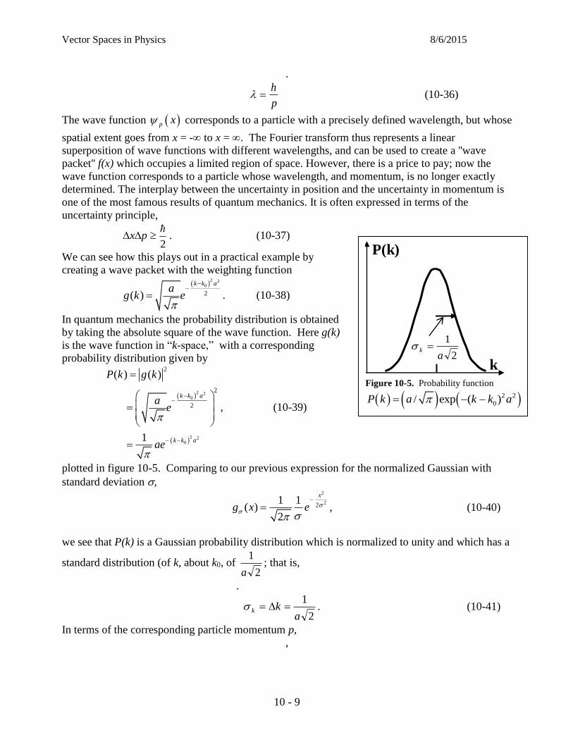
Vector Spaces in Physics 8/6/2015
10 - 9
.
p
h (10-36)
The wave function p x corresponds to a particle with a precisely defined wavelength, but whose
spatial extent goes from x = - to x = . The Fourier transform thus represents a linear
superposition of wave functions with different wavelengths, and can be used to create a ''wave
packet'' f(x) which occupies a limited region of space. However, there is a price to pay; now the
wave function corresponds to a particle whose wavelength, and momentum, is no longer exactly
determined. The interplay between the uncertainty in position and the uncertainty in momentum is
one of the most famous results of quantum mechanics. It is often expressed in terms of the
uncertainty principle,
2
px . (10-37)
We can see how this plays out in a practical example by
creating a wave packet with the weighting function
2 20
2( )
k k aa
g k e
. (10-38)
In quantum mechanics the probability distribution is obtained
by taking the absolute square of the wave function. Here g(k)
is the wave function in “k-space,” with a corresponding
probability distribution given by
2 20
2 20
2
2
2
( ) ( )
1
k k a
k k a
P k g k
ae
ae
, (10-39)
plotted in figure 10-5. Comparing to our previous expression for the normalized Gaussian with
standard deviation ,
2
221 1
( )2
x
g x e
, (10-40)
we see that P(k) is a Gaussian probability distribution which is normalized to unity and which has a
standard distribution (of k, about k0, of 2
1
a; that is,
.
2
1
akk . (10-41)
In terms of the corresponding particle momentum p,
,
k 2
1
ak
P(k)
k0
Figure 10-5. Probability function
2 2
0/ exp ( )P k a k k a

Vector Spaces in Physics 8/6/2015
10 - 10
2a
kp
(10-42)
where we have taken the rms deviation of the momentum distribution about its average value to
represent the uncertainty in p. We see that this distribution can be made as narrow as desired,
corresponding to determining the momentum as accurately as desired, by making a large.
Now, what is the corresponding uncertainty in position? We have to carry out the Fourier
transform to find out:
dkea
dkeea
dkekgxf
kxa
ikk
a
ikx
akk
ikx
2
20
2
220
2
2
2
2
1
2
1
)(2
1)(
(10-43)
We will work with the quantity in square brackets, collecting terms linear in k and performing an
operation called completing the square:
422
0
2
0
22
0
2
0
22
0
22
0
2
0
2
2
0
2
0
2
2
2
0
//2/
///2
/22
axaxikkaixkk
kaixkaixkaixkkk
kaixkkkkxa
ikk
(10-44)
The factor 22
0 / aixkk is the “completed square.” Substituting into the previous equation
gives
2
2
0
220
2
220
2/
2
422
0
2
0
22
0
2
2
1
//2/
2
1
)(2
1)(
a
x
xikaixkk
a
ikx
akk
ikx
eedkea
axaxikkaixkk
dkeea
dkekgxf
(10-45)
The quantity in square brackets is the integral of a Gaussian function and is equal toa
2; so we
have
2
2
0 21
)( a
x
xikee
axf
(10-46)
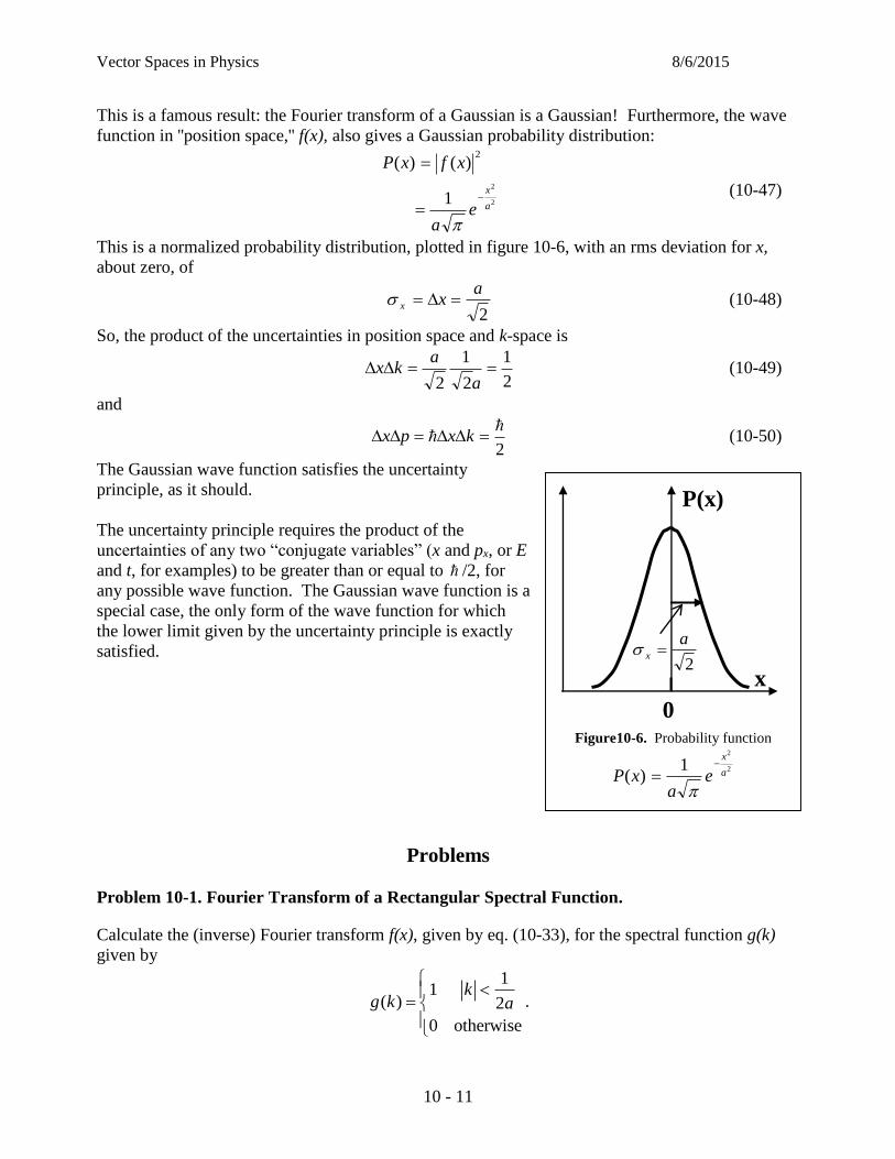
Vector Spaces in Physics 8/6/2015
10 - 11
This is a famous result: the Fourier transform of a Gaussian is a Gaussian! Furthermore, the wave
function in ''position space,'' f(x), also gives a Gaussian probability distribution:
2
2
1
)()(2
a
x
ea
xfxP
(10-47)
This is a normalized probability distribution, plotted in figure 10-6, with an rms deviation for x,
about zero, of
2
axx (10-48)
So, the product of the uncertainties in position space and k-space is
2
1
2
1
2
a
akx (10-49)
and
2
kxpx (10-50)
The Gaussian wave function satisfies the uncertainty
principle, as it should.
The uncertainty principle requires the product of the
uncertainties of any two “conjugate variables” (x and px, or E
and t, for examples) to be greater than or equal to /2, for
any possible wave function. The Gaussian wave function is a
special case, the only form of the wave function for which
the lower limit given by the uncertainty principle is exactly
satisfied.
Problems
Problem 10-1. Fourier Transform of a Rectangular Spectral Function.
Calculate the (inverse) Fourier transform f(x), given by eq. (10-33), for the spectral function g(k)
given by
11
( ) 2
0 otherwise
kg k a
.
x 2
ax
P(x)
0
Figure10-6. Probability function
2
2
1)( a
x
ea
xP

Vector Spaces in Physics 8/6/2015
10 - 12
Make a plot of the result, f(x) vs x. Indicate the values of x at the zero crossings.
Problem 10-2. Theorem Concerning the Dirac Delta Function. Use integration by parts to
prove the theorem given in eq. 10-19,
)()( afdxaxxf
(Here f' represents the derivative of f with respect to its argument, and ' represents the derivative
of with respect to its argument.)
Problem 10-3. Fourier Transform of a Gaussian. Calculate the Fourier transform (eq. 10-34)
of the wave function 2
20 2
1( )
x
ik x af x e ea
and verify that the result is
2 2
0
2( )
k k aa
g k e
.

Vector Spaces in Physics 8/6/2015
11 - 1
Chapter 11. Maxwell's Equations in Special Relativity.1
In Chapter 6a we saw that the electromagnetic fields E and B can be considered as
components of a space-time four-tensor. This tensor, the Maxwell field tensor F ,
transforms under relativistic "boosts" with the same coordinate-transformation matrix
used to carry out the Lorentz transformation on the space-time vector x . Since
then we have introduced vector differential calculus, centered around the gradient
operator . This operator, operating on the fields E and B and the potentials and
A , can be used to express the four Maxwell equations, giving a complete theory of the
electromagnetic field.
In this chapter we will start to put these equations into "covariant form," expressed in
terms equally valid in any Lorentz frame.
In Chapter 6a we introduced the position four-vector,
z
y
x
ct
x
the electromagnetic-field four-tensor,
1 1 10
10
10
10
x y z
x z y
y z x
z y x
E E Ec c c
E B Bc
F
E B Bc
E B Bc
,
and the Lorentz transformation matrix
0 0
0 0
0 0 1 0
0 0 0 1
,
which is used in the "usual tensor way" to transform vector and tensor indices from one
rest frame to another. Contraction of indices must always be between a upper and a
lower index, with the metric tensor
One may note factors of 1/c which were not present in the form of the field-strength tensor introduced in
Chapter 6a. This is a pesky issue of unit systems. The form given here gives the correct constants in the SI
system of units.

Vector Spaces in Physics 8/6/2015
11 - 2
1 0 0 0
0 1 0 0
0 0 1 0
0 0 0 1
g g
used to raise or lower indices. Upper indices are referred to as "contravariant" indices,
and lower indices, as "covariant" indices, referring to details of tensor analysis which we
hope to avoid discussing here.
More Four-Vectors
Let's just see some other combinations of a scalar and a three-vector which form four-
vectors.
four-momentum ,
four-current ,
four-potential: ,
1
four-gradient:
x
x y z
y
z
x
x y z
y
z
x
x y z
y
z
E
p cp p E p c p c p c
p c
p c
c
JJ J c J J J
J
J
AA A A A A
A
A
c t
x
y
z
1,
c t x y z
Note the cool scalar invariants formed by contracting certain of these vectors with
themselves.
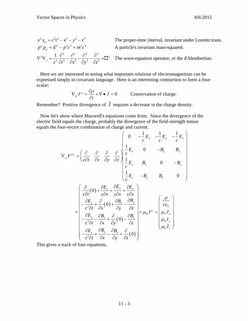
Vector Spaces in Physics 8/6/2015
11 - 3
2 2 2 2 2
2 2 2 2 4
2 2 2 22
2 2 2 2 2
The proper-time interval, invariant under Lorentz trans.
A particle's invariant mass-squared.
1The wave-equation operator, or the d'Al
x x c t x y z
p p E p c m c
c t x y z
embertian.
Here we are interested in seeing what important relations of electromagnetism can be
expressed simply in covariant language. Here is an interesting contraction to form a four-
scalar:
0 Conservation of charge.J Jt
Remember? Positive divergence of J requires a decrease in the charge density.
Now let's show where Maxwell's equations come from. Since the divergence of the
electric field equals the charge, probably the divergence of the field-strength tensor
equals the four-vector combination of charge and current.
2
2
2
1 1 10
10
10
10
0
0
0
0
x y z
x z y
y z x
z y x
yx z
yx z
y xz
y xz
E E Ec c c
E B Bc
Fc t x y z
E B Bc
E B Bc
EE E
c t c x c x c x
BE B
x y zc t
E BB
x y zc t
B BE
x y zc t
0
00
0
0
x
y
z
c
JJ
J
J
This gives a stack of four equations,

Vector Spaces in Physics 8/6/2015
11 - 4
0
0 0 0
0 0 0
0 0 0
1
x
z y x
y
x z y
z
y x z
Ec c
EB B J
y z t
EB B J
z x t
EB B J
x y t
Or, in old Earth-bound three-vector notation,
0
0 0 0
E
EB J
t
Here we have the two most complicated of Maxwell's equations, the source equation.
And you might notice that the famous "displacement-current" term, invented by Maxwell
to make the wave-equation work, has appeared as by magic:
displacement 0
EJ
t
.
Well, that is about as much excitement as most people can bear. But if you are good
for more - - - nobody really likes the curl. Let's set the four-curl of the field-strength
tensor equal to zero. This will of course involve the four-dimensional version of the
Levi-Civita totally anti-symmetric tensor,
1, an even permutation of 0123
1, an odd permutation of 0123
0 otherwise
Then
0 F
1 2 3
2 3 0
3 0 1
0 1 2
2 2 2
2 20 2
02 20 2
02 2
2
x y z
z y x
x y z
z y x
B B B
E E Bc c
E B Ec c
B E Ec c
The top line gives
0B
and the next three lines give

Vector Spaces in Physics 8/6/2015
11 - 5
BE
t
These complete Maxwell's equations. Good enough for one day.
1 http://www.phy.duke.edu/~rgb/Class/phy319/phy319/node135.html

Vector Spaces in Physics 8/6/2015
A - 1
Appendix A. Useful Mathematical Facts and Formulae
1. Complex Numbers
Complex numbers in general have both a real and an imaginary part. Here "i" represents
the square root of -1. If C represents a complex number, it can be written
C A i B , (AA-1)
with A and B real numbers. Thus,
Re
Im
A C
B C
(AA-2)
There is another representation of a complex number, in terms of its magnitude and
phase :
i
C e , (AA-3)
There is a very useful relation between the complex exponential representation and the
real trigonometric functions, the Euler equation:
cos sinie i (AA-4)
and the inverse relations,
cos2
sin2
i i
i i
e e
e e
i
(AA-5)
From equation (AA-4) one can deduce some useful special values for the complex
exponential:
2
1
1
i
i
e
e
(AA-6)
And from equation (AA-5) one easily deduces
cos cos
sin sin
A A
A A
(AA-7)
2. An Integrals and Two Identities.
2ue du
(AB-1)
sin sin cos sin cos
cos cos cos sin sin
A B A B B A
A B A B A B
(AB-2)
3. Power Series and the Small-Angle Approximation. It is especially convenient to
expand a function of a dimensionless variable as a power series when the variable can be
taken to be reasonably small. Some useful power series are given below.
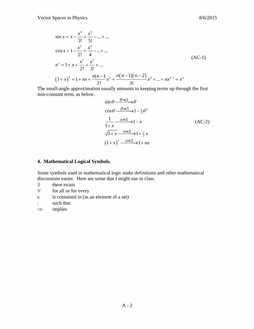
Vector Spaces in Physics 8/6/2015
A - 2
3 5
2 4
2 3
2 3 1
sin ... ...3! 5!
cos 1 .. ...2! 4
1 ...2! 3!
1 2( 11 1 ...
2! 3!
x
n n n
x xx x
x xx
x xe x
n n nn nx nx x x nx x
(AC-1)
The small-angle approximation usually amounts to keeping terms up through the first
non-constant term, as below.
212
12
1
1
1
1
1
sin
cos 1
11
1
1 1
1 1n
x
x
x
xx
x x
x nx
(AC-2)
4. Mathematical Logical Symbols.
Some symbols used in mathematical logic make definitions and other mathematical
discussions easier. Here are some that I might use in class.
there exists
for all or for every
is contained in (as an element of a set)
such that
implies

Vector Spaces in Physics 8/6/2015
B - 1
Appendix B. Using the P&A Computer System
The Physics and Astronomy Department maintains a rather complete computer system
for use by P&A faculty and students, located in TH 124. There are about 10 PC's running
Linux, and several others running Windows. The Linux machines are typical of the
platform used by many scientists for calculation. They should all have MatLab, Pyghon,
IDL and Mathematica installed locally. The information given below is rather volatile,
since the computer system is currently in a rapid state of change [written August 24,
2009.] Up-to-date information on this system can be obtained over the web at
http://www.physics.sfsu.edu/compsys/compsys.html
1. Logging on. To use the Physics and Astronomy computer system you need a system
account. Your instructor should request it, and when it is set up, you need to go to the
Department office to get your password, and to ask Peter Verdone (TH 104 or TH 212)
for a PIN to get you into TH 123. (If you have the password, a teacher or fellow student
will probably let you into the room, on a temporary basis.) We will assume that you have
your password and can get into TH 123.
(1) Choose one of the Linux machines. Pressing [enter] brings up a prompt for
entering your user name and password. A first-time user may receive some startup
messages.
(2) A desktop should open. If you only get a command window, start the desktop by
entering the command startx.
(3) From the desktop, open a terminal window by clicking on the third icon from the
left on the task bar at the bottom of the screen.
(4) I prefer to work from x-terminal windows. To open one of these, enter (from the
command line of the terminal window)
th123-22:bland% xterm &
NOTE: the first part of this instruction, th123-22:bland%, represents the command-line
prompt, and you do not type it. It will have your name, not bland. The command "xterm"
should open another window. The "&" character at the end of the line detaches the xterm
window from the window executing the instruction. Otherwise the terminal window is
useless as long as the xterm window is open.
2. Running Mathematica, MatLab and IDL.
You should be able to run these programs natively on all of the machines in TH123,
Linux or Windows. If your machine does not seem to have Mathematica, it might help to
connect to some other machine. For instance, to connect to th123-21, enter
th123-22:bland% ssh th123-21
Next, check to see that X-windows communication is open by running the clock window:
th123-21:bland% xclock &

Vector Spaces in Physics 8/6/2015
B - 2
A small window with a clock face should appear on your desktop. If it does not,
something is wrong. If xclock worked, you can run one of the big computation programs.
th123-21:bland% MatLab &
th123-21:bland% IDL
th123-21:bland% Mathematica
All of this can be done from Windows, too. You need to run an X-windows host, such
as xwin32 or xming, then connect to th123-22.sfsu.edu using a secure shell application
such as SSH. (See the Department computer system site,
http://www.physics.sfsu.edu/compsys/compsys.html, for more information.) Once
connected, open an xterm window, and continue as above. You will find that many
operations take a lot longer this way, due to the network connection. And with
Mathematica there are often problems with fonts. I recommend that you start the
semester working in the computer room, and set up remote access later if you want.
3. Mathematica.
This section gives some details on using Mathematica. Follow these instructions to load
and execute Mathematica. One warning - you may have to turn the "Num Lock" selection
off for Mathematica to respond to the keyboard.
th123-22:bland% mathematica &
A Mathematica icon should appear at once in the lower left-hand corner of the desktop,
and in a few seconds a Mathematica window will open. If instead you receive a message
telling you that the proper fonts are not installed, something is wrong. Try moving to
another workstation.
Here is a Mathematica command to enter, just to make sure that it is working:
Plot[Sin[x], {x, 0, 4 Pi}]
Execute the instruction with [shift][enter]. (Just pressing the [enter] key moves to a new
line, but does not execute the instruction.) A graph of two cycles of a sine wave should
appear.
To use the function for vector addition discussed in the text, carry out the following
commands from a terminal window:
th123-22:bland% ls Shows files on your home dir.
th123-22:bland% mkdir 385 Create directory for Ph 385
th123-22:bland% cd 385 Change to Ph 385 directory
th123-22:bland% cp ~bland/export/385/vectsum2.nb .
(Note the space and period at the end of the line.)
th123-22:bland% ls Should show the file vectsum2.nb

Vector Spaces in Physics 8/6/2015
B - 3
Now you can open the file vectsum2.nb with Mathematica and do the vector-addition
exercises.
If you prefer to work from home, and if you have Mathematica on your own computer,
you can download the file vectsum2.nb from the download page on the course website
and work on it there.

Vector Spaces in Physics 8/6/2015
C - 1
Appendix C. Mathematica
See Appendix B for instructions on accessing Mathematica on the Department computer
system. Here we will just present a routine for numerical addition of vectors. The
(magnitude, angle) representation for vectors is assumed.
1. Calculation of the vector sum using Mathematica. Today we rely increasingly on
"machines" to carry out laborious calculations like the preceding one for us.
Mathematica is one such machine, and we will use it in this course.
As a start, we will use Mathematica to carry out
the solution to the numerical example given in
Chapter 1, section B, illustrated in figures (1-4)
and (1-5). Here is the method. If we can
determine angle 1 of the triangle 1-2-3, we can
calculate the angle C (C = A - 1) and the
magnitude C of the sum vector (C2 = A2 + B2 – 2
A B cos 2, where 2 is determined from 2 + A
- B = 180). We will show how to do the
calculation using Mathematica. [The following
Mathematica commands are taken from the file
~bland/export/385/vectsum2.nb, also available on
the Ph 385 download page. Rather than typing
everything in, feel free to copy this file to your
directory and open it with Mathematica.] The first
command defines a Mathematica function which
calculates the vector sum of the two vectors A
and B
; the second shows a sample call to
this function; and the following line shows the answer by Mathematica. To run this
function yourself, just type in the commands exactly as shown, and press [Shift][Enter].
Vsum[{Amag_, Athdeg_, Bmag_, Bthdeg_}] := (
Ath = Athdeg*Pi/180. ;
Bth = Bthdeg*Pi/180. ;
Th2 = Pi - Ath + Bth;
Cmag = Sqrt[Amag^2 + Bmag^2 - 2 Amag Bmag Cos[Th2]];
CosTh1 = (Amag^2 + Cmag^2 - Bmag^2)/(2 Amag Cmag);
SinTh1 = Bmag*Sin[Th2]/Cmag;
Th1 = ArcTan[CosTh1, SinTh1];
Cth = Ath - Th1;
{Cmag, Cth*180. /Pi}
) <shift><enter>
Vsum[{10.,48.,14.,20.}] <shift><enter>
Out[2] = {23.3072,31.6205}
We will use this function for a variety of numerical calculations with vectors in the
(magnitude, angle) form.
Figure C-1.

Vector Spaces in Physics 8/6/2015
C - 2
2. Matrix operations in Mathematica.
3. Speed test for Mathematica. Here's a function to use to see how long Mathematica
takes to calculate the determinant of a matrix.
n=3
m=Table[Random[],{n},{n}];
Det[m]
Note: the semicolon at the end of the second line prevents printing out the matrix m. For
small values of m you could remove the semicolon, but for large values of m the printout
will take forever.
m={{2,4,3},{1,3,2},{1,3,1}} defining a matrix
MatrixForm[m] display as a rectangular array
cm multiply by a scalar
a . b matrix product
Inverse[m] matrix inverse
MatrixPower[m,n] nth power of a matrix
Det[m] determinant
Tr[m] trace
Transpose[m] transpose
Eigenvalues[m] eigenvalues
Engenvectors[m] eigenvectors
Eigenvalues[N[m]],Eigenvectors[N[m]] numerical eigenvalues and eigenvectors
m=Table[Random[],{3},{3}] 3x3 matrix of random numbers
<<Graphics` load graphics package
Solve[....,x] solve simultaneous linear equations
Plot3D[function(x,y),{x,...},{y ...}] 3-D plot
Table[...,{500},{500}] create stuff to plot
ListPlot[Abs[Eigenvalues[m]]] matrix eigenvalues
N[Pi,100] pi to a hundred places
Simplify[%] simplify the preceding answer
//N give numerical result
Table C-1. Some useful mathematical operations which Mathematica can carry out.
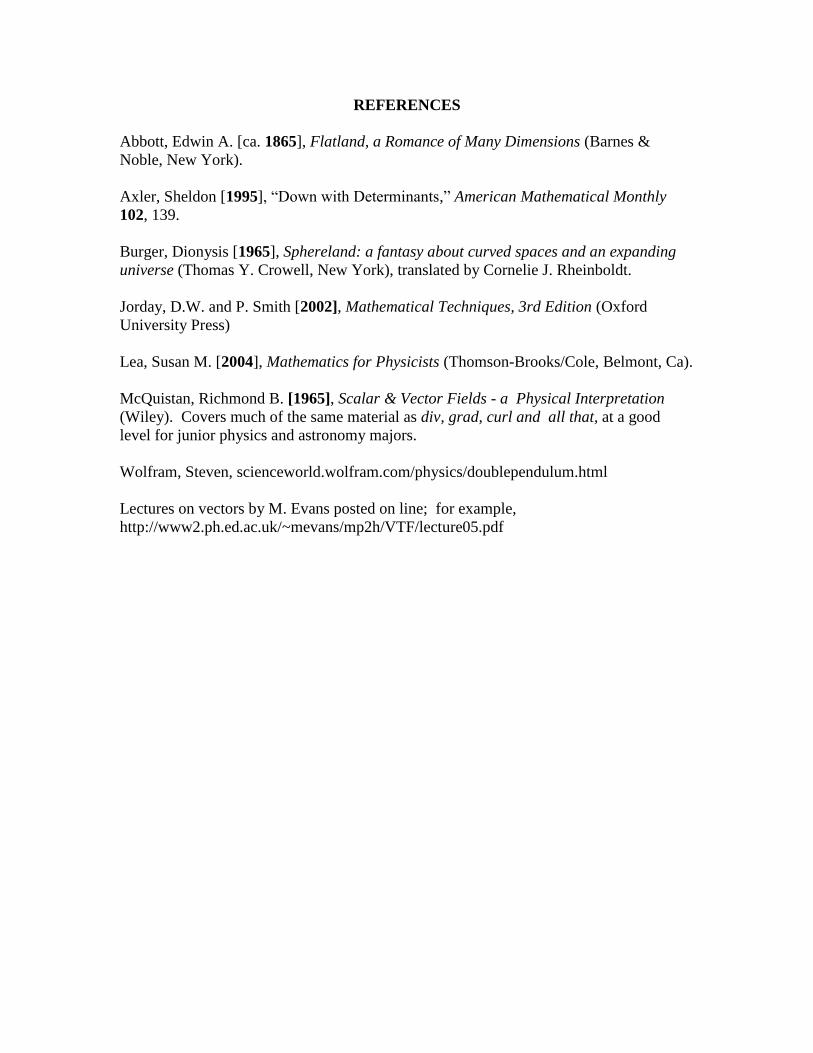
REFERENCES
Abbott, Edwin A. [ca. 1865], Flatland, a Romance of Many Dimensions (Barnes &
Noble, New York).
Axler, Sheldon [1995], “Down with Determinants,” American Mathematical Monthly
102, 139.
Burger, Dionysis [1965], Sphereland: a fantasy about curved spaces and an expanding
universe (Thomas Y. Crowell, New York), translated by Cornelie J. Rheinboldt.
Jorday, D.W. and P. Smith [2002], Mathematical Techniques, 3rd Edition (Oxford
University Press)
Lea, Susan M. [2004], Mathematics for Physicists (Thomson-Brooks/Cole, Belmont, Ca).
McQuistan, Richmond B. [1965], Scalar & Vector Fields - a Physical Interpretation
(Wiley). Covers much of the same material as div, grad, curl and all that, at a good
level for junior physics and astronomy majors.
Wolfram, Steven, scienceworld.wolfram.com/physics/doublependulum.html
Lectures on vectors by M. Evans posted on line; for example,
http://www2.ph.ed.ac.uk/~mevans/mp2h/VTF/lecture05.pdf


![b Topological Vector Spaces - WSEAS · vector spaces but is included in s topological vector spaces. Ibrahim [15] introduced the study of topological vector spaces. In 2018, Sharma](https://static.fdocuments.in/doc/165x107/5f131c8e356aa21b565c6315/b-topological-vector-spaces-wseas-vector-spaces-but-is-included-in-s-topological.jpg)