Vector Autoregressions

• VAR: Vector AutoRegression– Nothing to do with VaR: Value at Risk (finance)

• Multivariate autoregression

• Multiple equation model for joint determination of two or more variables

• One of the most commonly used models for applied macroeconometric analysis and forecasting in central banks

Two‐Variable VAR

• Two variables: y and x

• Example: output and interest rate

• Two‐equation model for the two variables

• One‐Step ahead model

• One equation for each variable

• Each equation is an autoregression plus distributed lag, with p lags of each variable

VAR(p) in 2 Variables

tptptt

ptpttt

exxx

yyyy

11112111

12121111

+++++

++++=

−−−

−−−

βββ

αααμ

L

L

tptptt

ptpttt

exxx

yyyx

22122121

22221212

+++++

++++=

−−−

−−−

βββ

αααμ

L

L

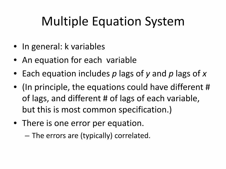
Multiple Equation System

• In general: k variables

• An equation for each  variable

• Each equation includes p lags of y and p lags of x

• (In principle, the equations could have different # of lags, and different # of lags of each variable, but this is most common specification.)

• There is one error per equation. – The errors are (typically) correlated.

Unrestricted VAR

• An unrestricted VAR includes all variables in each equation

• A restricted VAR might include some variables in one equation, other variables in another equation

• Old‐fashioned macroeconomic models (so‐called simultaneous equations models of the 1950s, 1960s, 1970s) were essentially restricted VARs– The restrictions and specifications were derived from simplistic macro theory, e.g. Keynesian consumption functions, investment equations, etc.

VAR Revolution

• Christopher Sims (1942‐) of Princeton University– 2011 Nobel Prize in Economics

• “Macroeconomics and Reality” (1980)– Sims argued that conventional macro models were “incredible” –they were based on non‐credible identifying assumptions

Sims and VARs

• Sims argued that the conventional models were restricted VARs, and the restrictions had no substantive justification– Based on incomplete and/or non‐rigorous theory, or intuition

• Sims argued that economists should instead use unrestricted models, e.g. VARs

• He proposed a set of tools for use and evaluation of VARs in practice.

Estimation

• Each equation estimated by OLS

tptptt

ptpttt

exxx

yyyy

11112111

12121111

+++++

++++=

−−−

−−−

βββ

αααμ

L

L

tptptt

ptpttt

exxx

yyyx

22122121

22221212

+++++

++++=

−−−

−−−

βββ

αααμ

L

L

Estimation in Stata

• To estimate a VAR in the variables y & x with lags 1 through p included– .varbasic y x, lags(1/p)

• For example, using gdp2013.dta and variables gdp and d.t12 with 3 lags– .gen rate=d.t12– .varbasic rate gdp, lags(1/3)

• Could also use– .var rate gdp, lags(1/3)

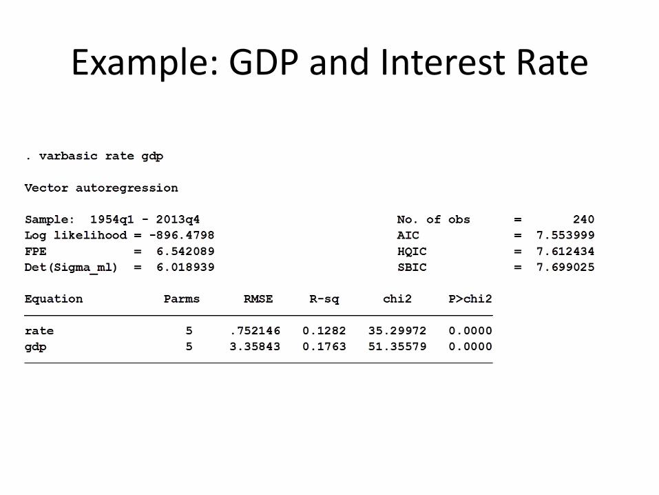
Example: GDP and Interest Rate

Example: GDP and Interest Rate

Order Selection

• A VAR(p) includes p lags of each variable in each equation

• In a two‐variable system, the number of coefficients in each equation is 1+2p– The total number is 2(1+2p)=2+4p

• In a k‐variable system, the number of coefficients in each equation is 1+kp– The total number is k(1+2p)=k+2kp

• How should p be selected?• Common approach: 

– Information criterion, primarily AIC

AIC and BIC for VAR Models

where L is log‐likelihood from model

• Select model with smallest AIC (or BIC)

( )kpkLAIC 222 ++−=

( ) ( )TkpkLBIC ln22 ++−=

Stata Implementation

• varsoc command

• To calculate information criterion for a VAR in variables x and y up to a maximum lag of pmax:– .varsoc x y, maxlag(pmax)

• Produces a convenient table

Example: GDP and Interest Rate

Result

• For this example– AIC selects p=3– BIC selects p=2

• Notice that the AIC value for p=3 in this table (AIC=7.572) is different from that obtained when we estimated the VAR(3) model (AIC=7.553).– This is because for the AIC comparison, all estimates are from a common sample, in this case excluding the first 8 observations since the maximum order is set to 8

• The varsoc command is correct

Let’s look at the VAR(3) estimates again.

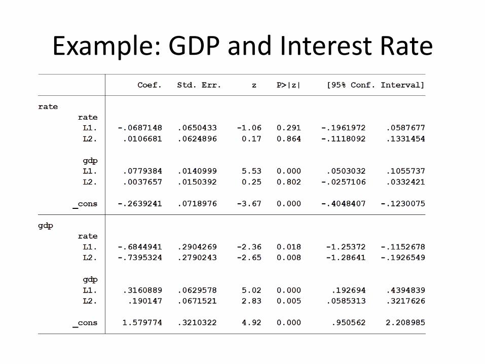
Example: GDP and Interest Rate

Interpretation

• It is difficult to interpret the large number of coefficients in the VAR model

• Main tools for interpretation– Impulse responses

Impulse Response Analysis

• VAR(1) with no intercept

• The impulse responses are the time‐paths of to y and x in response to shocks

tttt

tttt

exyxexyy

2121121

1111111

++=++=

−−

−−

βαβα

Impulse Response Analysis

• The errors may be correlated. 

• We “orthogonalize” them

tt

ttt

tt

uuuee

ue

21

212

11

+=+=

=

ρρ

Orthogonalized Model

• The shocks u1 and u2 are uncorrelated• The ordering matters

– The shock to y affects both y and x in period t– The shock to x affects only x in period t

• The impulse responses are the time‐paths of to y and x in response to the shocks u1 and u2

• Imagine y=0 and x=0. Set u1=1. Trace the history of y and x

ttttt

tttt

uuxyxuxyy

21121121

1111111

+++=++=

−−

−−

ρβαβα

Impulse Responses by Recursion

( ) ( )( ) ( )ρβαββααβα

ρβαββααβαρβαβα

βαβαρρβα

βα

2121211111212212213

2121111111112112113

21211211212

11111111112

21211

11111

1001100

+++=+=+++=+=

+=+=+=+=

=++==++=

xyxxyyxyxxyy

xy

Impulse Responses

• The impulse responses are these time‐paths of y and x due to the shocks u1 and u2

• They are found by this recursion formula

• They are functions of the estimated VAR coefficients

Impact of Shocks on Variables

• In a 2‐variable system, there are 4 impulse response functions– The effect on y of a shock to y (u1)

– The effect on y of a shock to x (u2)

– The effect on x of a shock to y (u1)

– The effect on x of a shock to x (u2)

• In a k‐variable system, there are k2 impulse response functions!

Stata Calculation

• Impulse response automatically calculated with varbasic command

• A kxk matrix of impulse response is created

GDP/Interest Rate Example

Interpretation

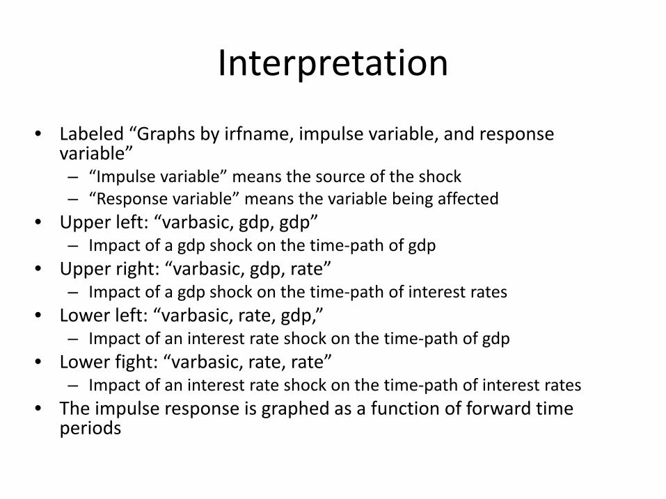
• Labeled “Graphs by irfname, impulse variable, and response variable”– “Impulse variable” means the source of the shock– “Response variable” means the variable being affected

• Upper left: “varbasic, gdp, gdp”– Impact of a gdp shock on the time‐path of gdp

• Upper right: “varbasic, gdp, rate”– Impact of a gdp shock on the time‐path of interest rates

• Lower left: “varbasic, rate, gdp,”– Impact of an interest rate shock on the time‐path of gdp

• Lower fight: “varbasic, rate, rate”– Impact of an interest rate shock on the time‐path of interest rates

• The impulse response is graphed as a function of forward time periods

Scale

• The graphs are all created on the same scale, so difficult to read

• It may be better to create graphs separate for each impulse response

• This creates the impulse response for the impact of a gdp shock on the time‐path of interest rates

GDP on GDP

GDP on Interest Rates

Interest Rates on Interest Rates

Interest Rates on GDP

3‐variable system

• Interest Rate Change (12‐month T‐Bill)

• Investment Growth Rate

• GDP Growth Rate

GDP/Investment/Interest Rate

Investment Shock on GDP

Investment Shock on Interest Rate

Interest Rate Shock on Investment

High Dimensional Estimation

• What if you have a situation where the number of regressions p exceeds the number of observations n ?

• Classic example: gene array data– Goal: Determine which gene causes cancer

– Number of regressors p = number of genes (5000)

– Number of observations p = 50 (or similar)

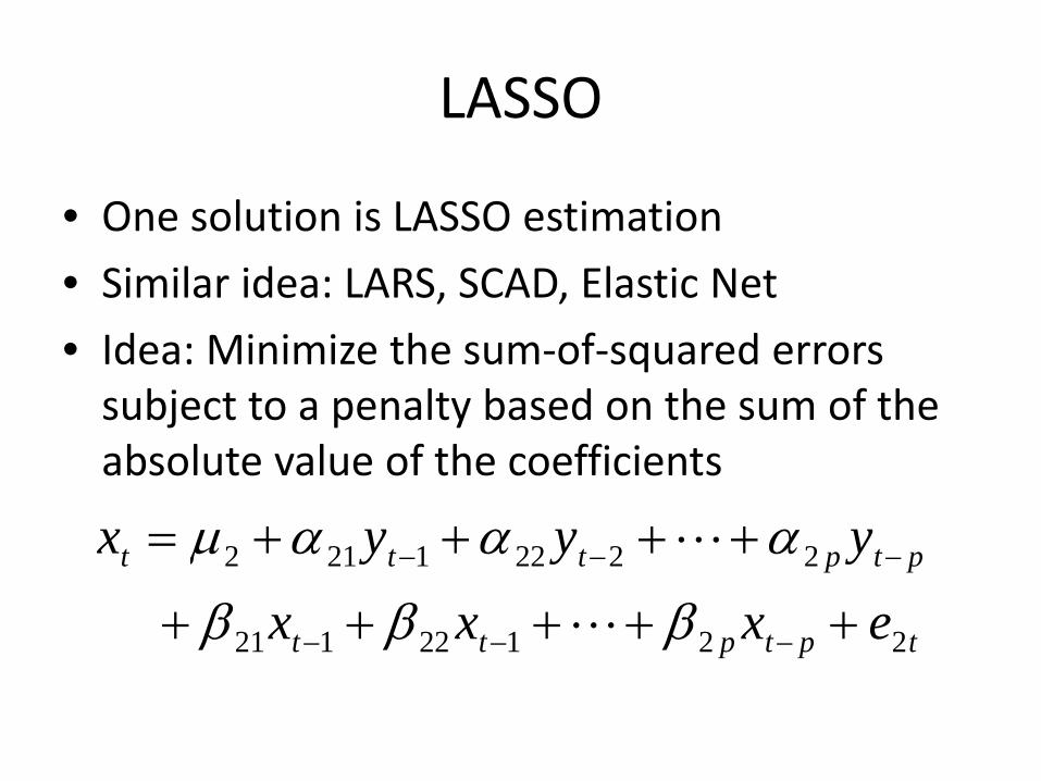
LASSO

• One solution is LASSO estimation

• Similar idea: LARS, SCAD, Elastic Net

• Idea: Minimize the sum‐of‐squared errors subject to a penalty based on the sum of the absolute value of the coefficients

tptptt

ptpttt

exxx

yyyx

22122121

22221212

+++++

++++=

−−−

−−−

βββ

αααμ

L

L

LASSOModel

Minimize sum‐of‐squared errors plus penalty

The penalty changes the problem.Most coefficient estimates are zero.

tptpttt exxxy +++++= βββμ L2211

( )

∑

∑

=

=

+

++++−

p

jj

T

tptpttt xxxy

1

1

22211

βλ

βββμ L

LASSO and Forecasting

• Lasso very popular in high‐dimensional statistics

• I haven’t yet seen Lasso being discussed in economic forecasting

• It is just a matter of time

• Not programmed in Stata

• If interested, I recommend the R package

Software after UW??

• You are unlikely to have access to Stata outside a university environment– Some corporations may have a few licenses– Non‐academic price is expensive

• Excel widely available– Often used for regression analysis in corporations– Highly limited & clumsy

• R is a viable option– Free, open‐source– Continuously updated– Popular among statisticians– http://www.r‐project.org/– A different style; may need to do more programming– Documentation sometimes limited