ORNL/TM/2012/621

VDRIVE Data Reduction and Interactive Visualization Software for Event Mode Neutron Diffraction Dr. Ke An Chemical and Engineering Materials Division Spallation Neutron Source Oak Ridge National Laboratory

DOCUMENT AVAILABILITY Reports produced after January 1, 1996, are generally available free via the U.S. Department of Energy (DOE) Information Bridge:

Web site: http://www.osti.gov/bridge Reports produced before January 1, 1996, may be purchased by members of the public from the following source: National Technical Information Service 5285 Port Royal Road Springfield, VA 22161 Telephone: 703-605-6000 (1-800-553-6847) TDD: 703-487-4639 Fax: 703-605-6900 E-mail: info@ntis.fedworld.gov Web site: http://www.ntis.gov/support/ordernowabout.htm Reports are available to DOE employees, DOE contractors, Energy Technology Data Exchange (ETDE) representatives, and International Nuclear Information System (INIS) representatives from the following source: Office of Scientific and Technical Information P.O. Box 62 Oak Ridge, TN 37831 Telephone: 865-576-8401 Fax: 865-576-5728 E-mail: reports@adonis.osti.gov Web site: http://www.osti.gov/contact.html

This report was prepared as an account of work sponsored by an agency of the United States Government. Neither the United States government nor any agency thereof, nor any of their employees, makes any warranty, express or implied, or assumes any legal liability or responsibility for the accuracy, completeness, or usefulness of any information, apparatus, product, or process disclosed, or represents that its use would not infringe privately owned rights. Reference herein to any specific commercial product, process, or service by trade name, trademark, manufacturer, or otherwise, does not necessarily constitute or imply its endorsement, recommendation, or favoring by the United States Government or any agency thereof. The views and opinions of authors expressed herein do not necessarily state or reflect those of the United States Government or any agency thereof.

ORNL/TM/2012/621 VDRIVE-DATA REDUCTION AND INTERACTIVE VISUALIZATION SOFTWARE FOR EVENT MODE NEUTRON DIFFRACTION Dr. Ke An CHEMICAL AND ENGINEERING MATERIALS DIVISION SPALLATION NEUTRON SOURCE OAK RIDGE NATIONAL LABORATORY Prepared by OAK RIDGE NATIONAL LABORATORY P.O. Box 2008 Oak Ridge, Tennessee 37831-6285 managed by UT-Battelle, LLC for the U.S. DEPARTMENT OF ENERGY under contract DE-AC05-00OR22725

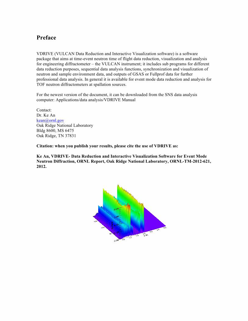
Preface

VDRIVE (VULCAN Data Reduction and Interactive Visualization software) is a software package that aims at time-event neutron time of flight data reduction, visualization and analysis for engineering diffractometer – the VULCAN instrument; it includes sub programs for different data reduction purposes, sequential data analysis functions, synchronization and visualization of neutron and sample environment data, and outputs of GSAS or Fullprof data for further professional data analysis. In general it is available for event mode data reduction and analysis for TOF neutron diffractometers at spallation sources. For the newest version of the document, it can be downloaded from the SNS data analysis computer: Applications/data analysis/VDRIVE Manual Contact: Dr. Ke An kean@ornl.gov Oak Ridge National Laboratory Bldg 8600, MS 6475 Oak Ridge, TN 37831 Citation: when you publish your results, please cite the use of VDRIVE as: Ke An, VDRIVE- Data Reduction and Interactive Visualization Software for Event Mode Neutron Diffraction, ORNL Report, Oak Ridge National Laboratory, ORNL-TM-2012-621, 2012.

ii

Contents Preface ................................................................................................................................. i 1 Flowchart and cheat sheet ......................................................................................... 1

2 Computer access ......................................................................................................... 3 3 VULCAN Data ............................................................................................................ 3

3.1 VULCAN data folder structure ...................................................................................... 3 3.2 Instrument files location .................................................................................................. 4 3.3 Download/upload your data ............................................................................................ 4 3.4 VDRIVE offline (beta) ..................................................................................................... 4

4 Data reduction, visualization and analysis with VDRIVE ...................................... 5 4.1 Load VDRIVE in IDL ...................................................................................................... 5 4.2 Data Reduction and Analysis Commands ...................................................................... 6

4.2.1 VDRIVERECORD .................................................................................................... 6 4.2.2 VDRIVECHOP ......................................................................................................... 6 4.2.3 VDRIVEMERGE ...................................................................................................... 7 4.2.4 VDRIVEBIN .............................................................................................................. 8 4.2.5 VDRIVEVIEW .......................................................................................................... 9 4.2.6 VDRIVEFIT ............................................................................................................ 10 4.2.7 VPEAK ..................................................................................................................... 13

5 Data Analysis with GSAS ........................................................................................ 14 5.1 Instrument files preparation ......................................................................................... 14

5.1.1 VULCAN instrument parameter file for GSAS ........................................................ 14 5.1.2 Name conventions and the locations of instrument files ........................................... 15 5.1.3 VDRIVECALI ......................................................................................................... 15 5.1.4 VDRIVEPRM .......................................................................................................... 15

5.2 VDRIVESPF ................................................................................................................... 15 5.3 VDRIVEGSAS ................................................................................................................ 17

Acknowledgement ............................................................................................................ 19 References ......................................................................................................................... 19 List of Figures Figure 1 Flowchart of VDRIVE. ...................................................................................................... 1 Figure 2 VDRIVE interface .............................................................................................................. 5 Figure 3 Raw histogram plots of GSAS pattern in the two banks. ................................................... 9 Figure 4 2D contour and 3D surface plots generated by VDRIVEVIEW. .................................... 10 Figure 5 Plot of single peak fit in one pattern by VDRIVEFIT. .................................................... 11 Figure 6 The fitting results from the VDRIVEFIT. ....................................................................... 12 Figure 7 Example of the VULCAN GSAS prm file. ...................................................................... 14

1

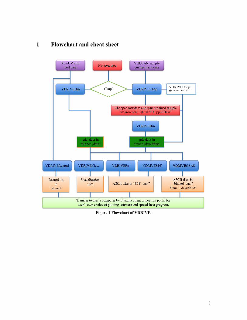
1 Flowchart and cheat sheet

Figure 1 Flowchart of VDRIVE.

2

VDRIVE cheat sheet Command line mode (requires IDL license on SNS server): Log on SNS linux machine (http://analysis.sns.gov) or local machine in the hutch with your XCAMS account (The one with which you submit proposal). Right click mouse and open a Terminal, type idl or idlde, then type @VDRIVE (case sensitive for these commands). Summarize, bin and view the record in one IPTS: (short name: VLOG) VDRIVERecord, IPTS=#### Chop, synchronize, and bin continuously collected data: (short name: CHOP) VDRIVECHOP, IPTS=####, RUNS=####, DBIN=####, BIN=1, Loadframe=1 [Furnace=1] Bin data to GSAS histogram files if not binned before: (short name: VBIN) VDRIVEBIN, IPTS=####, RUNS=####, RUNE=#### [, RUNV=####, CHOPRUN=####] [,ONEBANK=1] Note: using runv will normalize the gsas data with given instrument spectrum measured with vanadium, and use this for VDRIVESPF data analysis. View one GSAS raw pattern after binning as histogram data: (short name: VIEW) VDRIVEVIEW, IPTS=####, RUNS=#### [,CHOPRUN=####, RUNV=####, PCSENV=1] View sequential data in 2D contour and 3D surface: (short name: VIEW) VDRIVEVIEW, IPTS=####, RUNS=####, RUNE=#### [,CHOPRUN=####] [, MinV=#.#, MaxV=#.#, RUNV=####, NORM=1 , PCSENV=1] Conduct Gaussian single peak fit: (short name: VFIT) VDRIVEFIT, IPTS=####, RUNS=####, RUNE=#### [,CHOPRUN=####], LISTD=[#.#, #.#...], WIDTH=[#.#, #.#... ], [RUNR=####], [PCSENV=1, NORM=1] Conduct GSAS single peak fit: (short name: VSPF) VDRIVESPF, IPTS=####, RUNS=####, RUNE=#### [,CHOPRUN=####], [RUNR=####], [RUNV=####], [PCSENV=1], [NORM=1] Note: peak id file should be saved as peak.txt as the default in the binned folder. Conduct GSAS Rietveld refinement: (short name: GSAS) VDRIVEGSAS, IPTS=####, RUNS=####, RUNE=#### [,CHOPRUN=####], RUNM=#### [,BANK=[1,2]] Generate instrument parameter and instrument spectrum files (short name VBIN): VDRIVEBIN, RUNS=####, IPTS=####,TAG=’V’[,ONEBANK=1] VPEAK, IPTS=#### , RUNV=#### [,ONEBANK=1] VDRIVEPRM, IPTS=####, RUNV=####, FREQ= 30 (60 OR 20) [,ONEBANK=1] Generate instrument calibration files: (short name: CALI) VDRIVECALI, IPTS=4744, RUNP=####, RUNV=####, TAG=’Si’, FREQ=20 [,ONEBANK=1] VDRIVEGUI mode (no IDL license required): Application/data analysis/VDRIVEGUI, or open a Terminal and type VDRIVEGUI. In VDRIVEGUI, select VDRIVE functions in VDRIVE SUB tab to process data using the keywords above to process data.

3

2 Computer access What you need: 1 XCAMS account, the same one that you used in the IPTS system. If you do not have one follow this link to get one. (http://neutronsr.us). 2 Request access to computer resources (https://neutronsr.us/accounts/request.html) select, SNS user ( on-site and off-site ), then select VULCAN, finally type your IPTS number in the justification. Once you have an XCAMS account, you can go to http://analysis.sns.gov and follow the instruction for the remote window access.

3 VULCAN Data

3.1 VULCAN data folder structure Analyzed data are stored in a shared folder that all team members have the access. If you want to use VDRIVE offline, please keep the data structure of the ‘shared’ folder. /SNS/VULCAN/IPTS-1234/shared/ Under this folder you may find standard folders like below

binned_data/ GSAS file folder by created by VDRIVEBIN. Some analysis results may also be in the folder along with synchronized sample environment data. Results from VDRIVESPF and VDRIVEGSAS may also store in this folder.

Instrument/ Instrument parameter file (*.prm) and vanadium file (*-s.gda). Logs/ Sample environment files (loadframe, furnace and others). SPF_data/ Peak fitting data created by VDRIVEFIT and VDRIVESPF. Photos/ Photos captured by the camera computer. ChoppedData/ Chopped raw data by VDRIVECHOP. Raw data need to be

reduced by running VDRIVEBIN, or selecting bin=1 when executing VDRIVECHOP, copies of synchronized sample environment files are also in this folder.

Record.txt Record file generated by VDRIVERECORD. GSAS files are in ASCII format with three columns for each bank, and both banks data are saved in one files with data structure header as a separator. The three columns are, time of flight in ms (Tof), intensity (see the file header for normalization to vanadium), square root of intensity. The relationship between time of flight and d spacing is: Tof=d*DIFC+d^2*DIFA+ZERO DIFC, DIFA and Zero are instrument parameters which can be found in the instrument parameter file (*.prm). (see instrument parameter file section for details). Sample environment logs are in ASCII format with multiple columns. It has by default

4

timestamp, time elapsed, and variables (loadframe signals, or temperatures). Chopped sample environment files are synchronized with neutron timestamps. It has by default chopped runnumber, proton charge (for normalization by using pcsenv=1 keyword), and synchronized columns from sample environment files.

3.2 Instrument files location Processed instrument files and vanadium files are also in the VULCAN share folder. -------------------------------------------- /SNS/VULCAN/shared/Calibrationsfiles/Instrument/ Standards/ PRM/ Template/ --------------------------------------------

3.3 Download/upload your data After reduction/analysis, go to http://neutronsr.us/portal/ and log in the portal and select the folder above and then download/upload.

A fast way is to use an SFTP client to transfer data between your own computer and the data on server. FileZilla is a free one that works across different platforms. The server is analysis.sns.gov and the port for SFTP is 22.

3.4 VDRIVE offline (beta) VDRIVE visualization and data analysis subroutines can be used offline on a pc given the same folder scheme and proper installation of other party’s software. Now VDRIVE offline supports VDRIVEVIEW, VDRIVEFT, VDRIVESPF, VDRIVEGSAS. However, VDRIVERECORD, VDRIVEChop, VDRIVEBin and VDRIVECali data reduction routines are not recommended due to the raw and large data format of neutron data. Several configurations and a few of programs are needed to the successful execution of VDRIVE. On a Windows PC: Software requirements VDRIVEGUI.sav, download it from /SNS/VULCAN/shared/ IDL, www.exelisvis.com/idl/ (no license needed for VDRIVEGUI) GSAS, www.ccp14.ac.uk/solution/gsas/ MikTex, http://miktex.org GhostScript, http://www.ghostscript.com/download/ Adobe PDF Reader and MS Excel. Folder settings Folder paths of GSAS, MikTex, and GhostScript need manually to be set as environment paths. Download the IPTS “shared” folder GSAS data from the analysis computer, e.g.’c:\myvulcandata\shared’. Execution: Open VDRIVEGUI.sav by IDL. Add the keyword: UserDataDir=’c:\myvulcandata\shared’ in each of the commands. Although VDRIVE is available offline, it is recommended to use the Linux version due to the dependency of the programs settings above. On Mac (to be constructed)

5

4 Data reduction, visualization and analysis with VDRIVE

4.1 Load VDRIVE in IDL VDRIVE is based on the IDL. OS License OPEN Type first Then type Linux Yes Terminal idl or idlde (case sensitive) @VDRIVE (case

sensitive) Linux No Terminal VDRIVEGUI Linux No Application/data

analysis VDRIVEGUI

Use of VDRIVE In the terminal command console or idl workbench command console, type VDRIVE commands to perform data reduction, data fit, and data visualization. Or with the VDRIVEGUI, choose VDRIVE SUB tab, and type parameters line by line. Note: in the GUI, it does not support “/” in the command, should use “parameter=1” rather than “/parameter”

Figure 2 VDRIVE interface

6

4.2 Data Reduction and Analysis Commands

4.2.1 VDRIVERECORD Purpose: Extract run info and bin data with the default VDRIVEBIN configuration. Common use: VDRIVERECORD, IPTS=1000 The information of each run will be extracted from the xml file and stored in a text file /SNS/VULCAN/ IPTS-1000/shared/Record.txt. New data will be binned if not done before. At the end of the execution Record.txt file will be opened. It is also an easy way to locate the record file. Additional keywords:

Runs=#### Start run. Rune=#### End run. RecFile=’/path/file.txt’ Output records in a customized file.txt file under /path. Prm=’prmfile.prm’ Replace the Vulcan.prm comment line with the prmfile.prm in

GSAS files when NoBin=1 is not engaged. NoBin=1 Omit binning the data. NoShow=1 Omit showing the file at the end. Name=’name’ With Value keyword. Value=Value With Name extract a specific variable values to the ‘Value’ array

in current IDL workspace.

Other keywords taken by VDRIVEBIN.

4.2.2 VDRIVECHOP Purpose: Chop and bin continuously measured neutron data in time sequence under changing sample environment conditions. Common use: VDRIVECHOP, IPTS=1000, RUNS=2000, dbin=60, loadframe=1, bin=1 where, dbin is the chop step size in seconds; loadframe, is set when VULCAN loadframe is used for continuous loading experiment; bin=1, for binning data to GSAS file after slicing the data in time. GSAS data are stored at /SNS/VULCAN/IPTS-1000/shared/binned_data/2000/ along with the chopped sample environment files 2000sampleenv_chopped_start(mean or end).txt. Alternate for loadframe=1: furnace=1, or generic=1, when using VULCAN standard sample environment DAQ for the furnaces or others. For a customized sample environment file name, use SampleEnv=‘your sample file name.txt' (the customized sample environment file is stored in /SNS/VULCAN/IPTS-1000/shared/logs). If no sample environment is chosen or justchop=1 keyword is selected, no sample environment data synchronization will be executed. Other uses: To chop with customized time segments: VDRIVECHOP, IPTS=1000, RUNS=2000, pickdata="/SNS/VULCAN/IPTS-1000/shared/picktime.txt", bin=1, loadframe=1, pulsetime=1

7

where pickdata is the file name containing several selected time segments of the neutron data with the format of below (separated by tab and unit is seconds): ---------------------------- 1.00 10.00 20.01 30.00 40.01 50.00 … ---------------------------- Additional keywords:

Focus_EW=0 Bin data over each detector module. dt=###.## Time (s) between each chopped run, by default it equals dbin. If

less than dbin, each run will have overlapped neutron events. t0=###.## Time (s) offset from the start of neutron event files. te=###.## End time (s) to bin. Ndataset=### Number of chopped data set. Effective when the automatically

calculated data sets are more than Ndataset. Ndbin=### Number of time bins per cycle for stroboscopy. Ncycle=### Number of cycles to perform stroboscopy. Strobe=1 Set stroboscopy on. GSAS=1 Plot GSAS file after binning. Onelog=1 Read sample environment parameters from one log file. Accu=1 Accumulate data over chopped runs. PulseTime=1 For PickData, when PulseTime is used in the picktime.txt file. AppRun=#### Append chopped data to previously chopped data in

choprun=####. Will not work with Connect=1. Connect=1 Chop more than one runs and connect data after RUNS and data

are saved to RUNS’s chopped data folder. Will not work with AppRun.

Other VDRIVEBIN keywords when coupled with bin=1.

4.2.3 VDRIVEMERGE Purpose: Combine collected data. Data are combined from the runs of rest columns to the runs of the first column in the runfile.txt. Common use: VDRIVEMERGE, IPTS=1000, RUNFILE="/SNS/VULCAN/IPTS-1000/shared/runfile.txt", CHOPRUN=2 The combined data are saved to /SNS/VULCAN/IPTS-1000/shared/chopped_data/2/ To bin the data combined by VDRIVEMERGE: VDRIVEBIN, IPTS=1000, CHOPRUN=2 GSAS files are stored in /SNS/VULCAN/IPTS-1000/shared/binned_data/2/ Example of the tab delimited runfile.txt: ---------------------------- 1001 1002 1003 1004 1005 1006 1007 1008 1009 1010

8

… ---------------------------- Additional keywords: NONE

4.2.4 VDRIVEBIN Purpose: Bin collected data or chopped data by VDRIVECHOP to GSAS files. Common use: For typical mapping experiments or single run: VDRIVEBIN, IPTS=1000, RUNS=2000, RUNE=2099 GSAS files are stored in /SNS/VULCAN/IPTS-1000/shared/binned_data/ For chopped files created by VDRIVECHOP: VDRIVEBIN, IPTS=1000, CHOPRUN=2000, RUNS=1, RUNE=100 GSAS files are stored in /SNS/VULCAN/IPTS-1000/shared/binned_data/2000/ Additional keywords:

BINW=0.005 The logarithm bin step size of TOF and its default is 0.001. SKIPXML=1 Some parameters from xml file will be written in the GSAS files

as comments, which are convenient for using SmartsRunRep in SMARTSWare.

FOCUS_EW=0 For 6-module data binning. RUNV=5000 Normalize data over smoothed vanadium file in /Instrument

folder, and used for VDRIVESPF when normalized intensity is an output option.

IParm=’prmfile.prm’ Replace the Vulcan.prm in comment line with the customized prmfile.prm string in GSAS files.

FullProf=1 Output FullProf files. NoGSAS=1 Omit GSAS files. PlotFlag=1 Plot histogram after binning. OneBank=1 Bin banks data to one histogram. NoMask=1 Bin bad pixels too. Tag=’Si’ Bin a Si calibration powder. If ‘CeO2’ is chosen, bin a CeO2

calibration powder. If ‘V’ is chosen, bin a vanadium data. Focus_tof=1 Omit time focusing. BinFolder=’/folder’ Bin data to a specific folder.

Other variations: VDRIVEBINP Purpose: Bin histograms with bundled pixels. e.g. for application of single crystal patterns. Common use: VDRIVEBINP, IPTS=1000, RUNS=1, RUNE=100, PBinsize=8 where, PBinsize is the number of pixels to be bundled/binned into one histogram, and the default is 8, which means every 8 vertical pixels of each VULCAN detector module will be binned into

9

one histogram, thus creating 154 GSAS files for each module. Therefore it will generate lots of GSAS files. Note: Data is not time-focused when using VDRIVEBINP. VDRIVEBINH Purpose: Bin 154 horizontal pixels into one individual histogram, so 7 histograms for each module, and total 42 histograms for 1 chopped data. All data will be saved as 42-bank spectrum (time focused) in one GSAS file. VDRIVEBINV Purpose: Bin 8 vertical pixels into 1 histogram, 154 histograms for each module, 154*6 GSAS files same as for VDRIVEBINP when PBinsize=8. However each GSAS file is time focused.

4.2.5 VDRIVEVIEW Purpose: Visualize data in 2D, 3D plots. Common use: To view one GSAS pattern: VDRIVEVIEW, IPTS=1000, RUNS=1, plot=1

Figure 3 Raw histogram plots of GSAS pattern in the two banks.

To view sequential GSAS patterns in 2D and 3D: VDRIVEVIEW, IPTS=1000, RUNS=1, RUNE=50 To view sequential GSAS patterns of chopped data in 2D and 3D: VDRIVEVIEW, IPTS=1000, CHOPRUN=2000, RUNS=1, RUNE=50

10

Figure 4 2D contour and 3D surface plots generated by VDRIVEVIEW.

Additional keywords:

RUNV=5000 Normalize GSAS pattern with instrument spectrum by the vanadium pattern.

TOTALCOUNTS=1 Normalize with total counts of each bank. PCSENV=1 For chopped data, normalize chopped data with proton charge

(beam charge). MinV=0.7, MaxV=2.7 Define the display range in d space. Position=1, SENV=5 Show the 6th variable (starting from 0) as the vertical axis in the

contour and surface plots. Can be any Nth column in the chopped sample environment files.

Norm=1 Normalize proton charge from xml file of single run measurement (differs from pcsenv for chopped runs).

Tof=1 Show x in time of flight. Angle=1 Show x in 2 theta angle. Q=1 Show x in Q. Lambda=1 Show x in wavelength. PlotGSAS=1 Show individual GSAS pattern. ClearPlot=1 Reset plotted windows by previous execution of

VDRIVEVIEW. XML=1 When Position=’varialbe_name’ is set, show the value of the

variable from xml file in the vertical axes. SameScale=1 Show two banks data in same scale. Merge=1 Show two banks data in one window. Log=1 Plot intensity in logarithm. DIFC=[16370,16372] Manually input DIFCs of the two banks.

4.2.6 VDRIVEFIT Purpose: Gaussian single peak fit and results visualization. Common use: For one GSAS pattern fit: VDRIVEFIT, IPTS=1000, RUNS=1, listd=[2.60,2.45,1.89,1.6,1.47], width=[0.035, 0.03, 0.03, 0.03, 0.03], plot=1

11

where, listd is the list of initial guess of the peak position, width is the data range of the peak in d-space for each peak, can be one value for all peaks, or an array of values for each peak;

Figure 5 Plot of single peak fit in one pattern by VDRIVEFIT.

For sequential GSAS patterns fit: VDRIVEFIT, IPTS=1000, RUNS=1, RUNE=50, RUNR=1, listd=[2.04, 1.76, 1.243, 1.06], width=[0.03,0.03,0.03,0.02], UpdateP=1 or for chopped GSAS patterns fit VDRIVEFIT, IPTS=1000, ChopRun=2000, RUNS=1, RUNE=50, RUNR=1, listd=[2.04, 1.76, 1.243, 1.06], width=[0.03,0.03,0.03,0.02], UpdateP=1 where RUNR is the strain reference run, otherwise, d-space will be the only output; UpdateP=1, peak center of previous run will be used as the guess of current run.

12

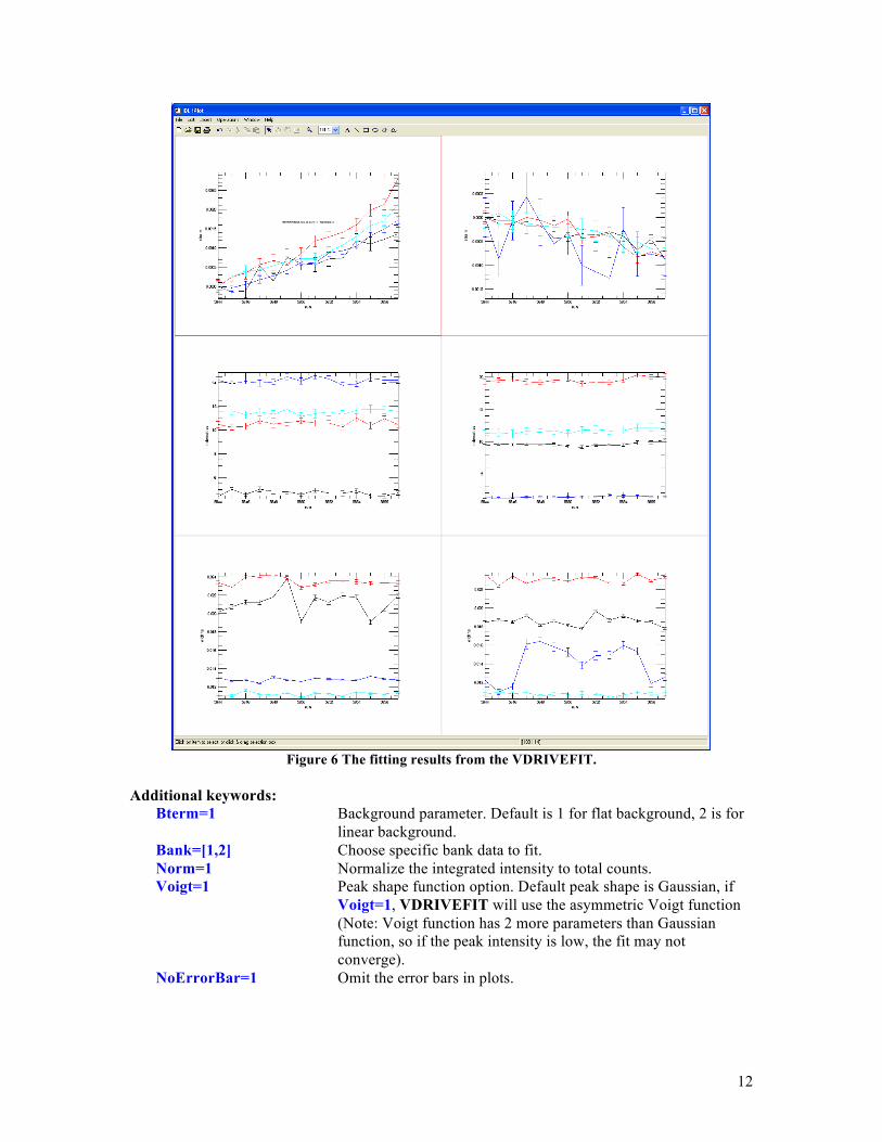
Figure 6 The fitting results from the VDRIVEFIT.

Additional keywords:

Bterm=1 Background parameter. Default is 1 for flat background, 2 is for linear background.

Bank=[1,2] Choose specific bank data to fit. Norm=1 Normalize the integrated intensity to total counts. Voigt=1 Peak shape function option. Default peak shape is Gaussian, if

Voigt=1, VDRIVEFIT will use the asymmetric Voigt function (Note: Voigt function has 2 more parameters than Gaussian function, so if the peak intensity is low, the fit may not converge).

NoErrorBar=1 Omit the error bars in plots.

13

Position=1, SENV=5 Show the 6th variable (starting from 0) as the vertical axis in the contour and surface plots. Can be any Nth column in the chopped sample environment files.

Log=1 Take logarithm of the intensity and then perform the fit. Pcsenv=1 Normalize the intensity by the proton charge in the chopped

sample environment file. Sho=1 Show the fitting results in the command console. Showbad=1 Show the bad fitting results in plots.

Peak positions, intensities, peak widths and strains of each peak are stored in ASCII files RUNS_1.txt and RUNS_2.txt under /SNS/VULCAN/IPTS-####/shared/SPF_data. Results should be checked. Usually if there are some exotic points, it means either the statistics of these data are poor, or some initial parameters such as peak position or width should be adjusted. If peaks are too close, initial values of original position and width are important. This command is not recommended for overlapping peaks fitting.

4.2.7 VPEAK Purpose: Process vanadium diffraction peak and data noise. Common use: VPEAK, IPTS=1000, RUNV=5000 Additional keyword:

Nsmooth =51 The number of points to be used in the boxcar smoothing algorithm, the bigger the smoother.

OneBank=1 When all banks’ data are binned as one bank data.

The smoothed data is named as ####-s.gda and located at /SNS/VULCAN/IPTS-1000/shared/Instrument as well as a copy in the VULCAN shared folder /SNS/VULCAN/shared/Calibrationsfiles/Instrument/Standards/.

14

5 Data Analysis with GSAS

5.1 Instrument files preparation

5.1.1 VULCAN instrument parameter file for GSAS

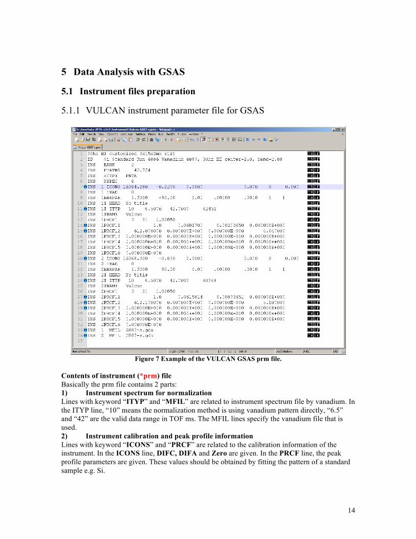
Figure 7 Example of the VULCAN GSAS prm file.

Contents of instrument (*prm) file Basically the prm file contains 2 parts: 1) Instrument spectrum for normalization Lines with keyword “ITYP” and “MFIL” are related to instrument spectrum file by vanadium. In the ITYP line, “10” means the normalization method is using vanadium pattern directly, “6.5” and “42” are the valid data range in TOF ms. The MFIL lines specify the vanadium file that is used. 2) Instrument calibration and peak profile information Lines with keyword “ICONS” and “PRCF” are related to the calibration information of the instrument. In the ICONS line, DIFC, DIFA and Zero are given. In the PRCF line, the peak profile parameters are given. These values should be obtained by fitting the pattern of a standard sample e.g. Si.

15

More information of the instrument parameter files can be found in the GSAS manual. If needed, instrument files can be created/updated by refining the standard data Si every cycle along with the smoothed vanadium data. Or one can look for one instrument file that has the same configuration (guide, chopper, lambda center, lambda width, and sample environment) from /SNS/VULCAN/shared/Calibrationfiles/Instrument/PRM. The files are updated usually once in a cycle.

5.1.2 Name conventions and the locations of instrument files VULCAN GSAS instrument files are named according to the vanadium run number, such as Vulcan-5000-s.prm, where 5000 is the vanadium run number, and “-s” means the vanadium pattern has been smoothed by VPEAK. For each user project, the instrument files, including the prm file and the smoothed vanadium data, should be stored in the IPTS folder /SNS/VULCAN/IPTS-####/shared/Instrument. The template prm files are in the folder /SNS/VULCAN/shared/Calibrationfiles/PRM/Template. Note: User may have more than one instrument prm files depending on the configurations used in the experiment.

5.1.3 VDRIVECALI Purpose: Generate instrument calibration files from Si and vanadium measurements. Common use: VDRIVECALI, IPTS=4744, RUNP=12474, RUNV=12475, TAG=’Si’, Freq=20 This example is based on high intensity (HI) 20Hz chopper setting Si powder measurement RUNP=12474, and the corresponding vanadium measurement RUNV=12735. Instrument parameter file Vulcan-12735-s.prm will be created in /SNS/VULCAN/shared/Calibrationfiles/Instrument/PRM/ and also the template instrument file Vulcan-template-HI.prm is created or updated under /SNS/VULCAN/shared/Calibrationfiles/Instrument/Template Additional keywords:

OneBank=1 For one bank calibration when two banks data are binned as one. The files will be saved in ‘/1bk’ under those instrument folders.

5.1.4 VDRIVEPRM Purpose: Generate user specific instrument files from calibration (template) files. Common use: VDRIVEPRM, IPTS=1000, RUNV=5000, FREQ=20 (or 30, 60)[, ONEBANK=1] Vulcan-5000-s.prm and 5000-s.gda will be created in /SNS/VULCAN/IPTS-1000/shared/Instrument.

5.2 VDRIVESPF Purpose: Use GSAS for single peak fit including overlapping peaks. Common use: For typical mapping experiments: VDRIVESPF, IPTS=1000, RUNS=1, RUNE=100, RUNR=1, RUNV=5000[ ,Normalize=1]

16

For sequential GSAS files of chopped run: VDRIVESPF, IPTS=1000, CHOPRUN=2000, RUNS=1, RUNE=100, RUNR=1, RUNV=5000, PCSENV=1 Required files: Peak ID file (peak.txt), instrument parameter file (*.prm), and instrument spectrum file by vanadium (*-s.gda). *.prm and *-s.gda should be under the instrument folder. The peak ID file is recommended to be named as peak.txt under the (chopped) GSAS data folder. An example of the peak.txt file is below:

------------------------------------------------------------------ 1 110 1 2.02692 0.0300000 $1 310 1 0.906467 0.0250000 $2 110 1 2.02692 0.0300000 $2 200 1 1.43325 0.0300000 2 211 1 1.17024 0.0200000 $2 220 1 1.01346 0.0300000 -----------------------------------------------------------------

The names of the columns are: Bank ID, name of the peak, number of peaks, estimated peak position (in d), estimated peak range (in d). $ sign is for comment line. For overlapped peaks, which are too close to perform single peak fit, alternate the first peak column value for the purpose of fitting and outputting the corresponding results. An example is given below:

-------------------------------------------------------------------------- $ Fit the first peak 1 peak1 2 2.02345 2.03456 0.04 $ Fit the second peak 1 peak2 2 2.03456 2.02345 0.04 --------------------------------------------------------------------------

Additional keywords:

peakFile=’peak.txt’ For customized peak ID file name other than the default one. Runfile=’file.txt’ Fit runs in a text file, one run per line. UpdataP=1 Take previous run as the peak parameters guess for current run. prmFile=’ prmfile.prm’ Use different prm file. myRefine=’Refine.txt’ Use a customized refinement steps in a macro file. NoErrorBar=1 Omit the error bars in plots. UserDataDir=’/folder’ Direct the data in a specific folder. Plotdata=0 Omit the plots. Showbad=1 Show bad refinement results in the plots. Pcsenv=1 Spectrum divided by proton charge, not with monitor. Monitor=1 Spectrum divided by monitor 2, not with pcsenv. Normalization=1 Normalize to Vanadium file (with runv).

17

Result file list:

VDriveSPF-2000-1-50-bk1.txt Peak positions, widths, intensities, and strains (in refinement folder as well as a copy in SPF_data folder).

VDriveSPF-2000-1-50-bk1.pdf Fitting plots for quality check (in refinement folder as well as a copy in SPF_data folder).

VDriveSPF-2000-1-50-bk1.log Refinement histories.

5.3 VDRIVEGSAS Purpose: Use GSAS for Rietveld Refinement based on a source run. Common use: For typical runs: VDRIVEGSAS, IPTS=1000, RUNS=1, RUNE=100, RUNM=1, BANK=1 For GSAS files from chopped data: VDRIVEGSAS, IPTS=1000, CHOPRUN=2000, RUNS=1, RUNE=100, RUNM=1, BANK=1 Required files: Instrument parameter file (*.prm), instrument spectrum file by vanadium (*-s.gda) and a source run (RUNM) which has been refined well by GSAS are required and stored the GSAS data folder before the execution of this command. The source files will define the refinement scheme of Rietveld refinement in GSAS. If the source RUNM is 1, VDRIVEGSAS needs GSAS EXP files 1_1.EXP and 1_2.EXP for bank 1 and 2, respectively. Additional keywords:

Nphase=2 Number of phases in the GSAS data. UserDataDir=’/folder’ Direct the data in a specific folder. Runfile=’listfile.txt’ Fit runs in a text file, one run per line. Title=’Title’ Title for all GSAS refinement.

Result file list:

VDriveGSAS-2000-1-50-bk1.txt Lattice parameters, strains. VDriveGSAS-2000-1-50-bk1.pdf Refinement plots for quality check VDriveGSAS-2000-1-50-bk1-atom.txt Atom occupancies if turned on. VDriveGSAS-2000-1-50-bk1-profile.txt Peak profile parameters. VDriveGSAS-2000-1-50-bk1.log Refinement histories.

Create a source run for VDRVIEGSAS Open Terminal Type expgui Direct to your “binned_folder” then type ####_1.EXP, then click “Create” button Type a string for the exp file title. Click “Add Phase” Select the way to add new phase ( either by previous EXP file, or CIF file) Point to the file containing crystal phase information Click “Continue” Modify the atom name properly and click “Add Atoms” In “Powder” tab, click “Add New Histogram” In Data file, click “Select” In Instrument file, click “Select” ( better copy the instrument files to the binned_data folder)

18

Follow the GSAS manual to perform a good refinement of the data. Perform same way to generate source run for bank 2 by simply change ####_1.EXP to ####_2.EXP.

19

Acknowledgement

The computer and software supports from Harley Skorpenske, Ling Yang, Jean C. Bilheux, John Quigley, Kyle Anderson, and Jason Hodges are acknowledged. The Spallation Neutron Source is a user facility at Oak Ridge National Laboratory sponsored by the Office of Basic Energy Science, the Office of Science, the Department of Energy, USA. Oak Ridge National Laboratory is managed by UT-Battelle, LLC, for the U.S. Dept. of Energy under contract DE-AC05-00OR22725.

References

1. A.C. Larson and R.B. Von Dreele, "General Structure Analysis System (GSAS)", Los Alamos National Laboratory Report LAUR 86-748 (2000). 2. IDL, http://www.exelisvis.com/