VAW Mitteilung 177: INVESTIGATION OF WATER .... ETH NO. 14835 INVESTIGATION OF WATER DRAINAGE...
158
DISS. ETH NO. 14835 I NVESTIGATION OF WATER DRAINAGE THROUGH AN ALPINE GLACIER BY TRACER EXPERIMENTS AND NUMERICAL MODELING A dissertation submitted to the SWISS FEDERAL I NSTITUTE OF TECHNOLOGY ZURICH for the degree of Doctor of Natural Sciences presented by THOMAS SCHULER Dipl. Hydr. Universität Freiburg im Breisgau born 19. March 1971 in Bühl/ Baden (Germany) accepted on the recommendation of Prof. Dr. H.-E. Minor, examiner Dr. U. H. Fischer, co-examiner Dr. G. H. Gudmundsson, co-examiner Dr. L. N. Braun, co-examiner 2002
Transcript of VAW Mitteilung 177: INVESTIGATION OF WATER .... ETH NO. 14835 INVESTIGATION OF WATER DRAINAGE...

DISS. ETH NO. 14835
INVESTIGATION OF WATER DRAINAGE
THROUGH AN ALPINE GLACIER BY
TRACER EXPERIMENTS AND NUMERICAL MODELING
A dissertation submitted to the
SWISS FEDERAL INSTITUTE OF TECHNOLOGY ZURICH
for the degree ofDoctor of Natural Sciences
presented by
THOMAS SCHULER
Dipl. Hydr. Universität Freiburg im Breisgau
born 19. March 1971
in Bühl/ Baden (Germany)
accepted on the recommendation of
Prof. Dr. H.-E. Minor, examiner
Dr. U. H. Fischer, co-examiner
Dr. G. H. Gudmundsson, co-examiner
Dr. L. N. Braun, co-examiner
2002
Contents
Contents . . . . . . . . . . . . . . . . . . . . . . . . . . . . . . . . . . . . . . . . . ii
List of Figures . . . . . . . . . . . . . . . . . . . . . . . . . . . . . . . . . . . . . . v
List of Tables . . . . . . . . . . . . . . . . . . . . . . . . . . . . . . . . . . . . . . viii
List of Symbols . . . . . . . . . . . . . . . . . . . . . . . . . . . . . . . . . . . . . x
Abstract . . . . . . . . . . . . . . . . . . . . . . . . . . . . . . . . . . . . . . . . . xv
Zusammenfassung . . . . . . . . . . . . . . . . . . . . . . . . . . . . . . . . . . . . xvii
1 Introduction 1
1.1 Significance of glacial hydrology . . . . . . . . . . . . . . . . . . . . . . . . . 1
1.1.1 Glacier dynamics . . . . . . . . . . . . . . . . . . . . . . . . . . . . . 1
1.1.2 Glacial discharge . . . . . . . . . . . . . . . . . . . . . . . . . . . . . 2
1.2 Techniques of investigation . . . . . . . . . . . . . . . . . . . . . . . . . . . . 3
1.3 Study area: Unteraargletscher . . . . . . . . . . . . . . . . . . . . . . . . . . . 3
1.4 Objectives . . . . . . . . . . . . . . . . . . . . . . . . . . . . . . . . . . . . . 5
1.5 Structure of the thesis . . . . . . . . . . . . . . . . . . . . . . . . . . . . . . . 7
2 Glacial hydrology: a process review 9
2.1 Runoff generation at the surface . . . . . . . . . . . . . . . . . . . . . . . . . 9
2.1.1 Surface energy balance . . . . . . . . . . . . . . . . . . . . . . . . . . 9
2.1.2 Importance of energy fluxes . . . . . . . . . . . . . . . . . . . . . . . 10
2.2 Water flow through the glacier . . . . . . . . . . . . . . . . . . . . . . . . . . 11
2.2.1 Firn and supraglacial hydrology . . . . . . . . . . . . . . . . . . . . . 12
2.2.2 Englacial passageways . . . . . . . . . . . . . . . . . . . . . . . . . . 13
2.2.3 Subglacial hydrology . . . . . . . . . . . . . . . . . . . . . . . . . . . 14
2.3 Characteristics of glacial runoff . . . . . . . . . . . . . . . . . . . . . . . . . . 17
2.3.1 Variability due to meltwater generation processes . . . . . . . . . . . . 18
2.3.2 Variability due to routing processes . . . . . . . . . . . . . . . . . . . 18
ii

CONTENTS iii
3 Water balance 21
3.1 Methods . . . . . . . . . . . . . . . . . . . . . . . . . . . . . . . . . . . . . . 21
3.1.1 Meteorological records . . . . . . . . . . . . . . . . . . . . . . . . . . 21
3.1.2 Determination of surface melt . . . . . . . . . . . . . . . . . . . . . . 22
3.1.3 Glacial runoff . . . . . . . . . . . . . . . . . . . . . . . . . . . . . . . 27
3.2 Results . . . . . . . . . . . . . . . . . . . . . . . . . . . . . . . . . . . . . . . 29
3.2.1 Input into glacial system . . . . . . . . . . . . . . . . . . . . . . . . . 29
3.2.2 Output from glacial system . . . . . . . . . . . . . . . . . . . . . . . . 30
3.2.3 Water balance . . . . . . . . . . . . . . . . . . . . . . . . . . . . . . . 31
3.2.4 Rainfall-induced outburst . . . . . . . . . . . . . . . . . . . . . . . . . 34
3.3 Discussion . . . . . . . . . . . . . . . . . . . . . . . . . . . . . . . . . . . . . 34
4 Tracer tests and their analysis 37
4.1 Principles of tracer experiments . . . . . . . . . . . . . . . . . . . . . . . . . 37
4.1.1 Requirements on tracers . . . . . . . . . . . . . . . . . . . . . . . . . 37
4.1.2 Properties of fluorescent dyes and other tracers . . . . . . . . . . . . . 38
4.2 Transport models . . . . . . . . . . . . . . . . . . . . . . . . . . . . . . . . . 38
4.2.1 Advection-dispersion model . . . . . . . . . . . . . . . . . . . . . . . 39
4.2.2 Mobile-immobile model . . . . . . . . . . . . . . . . . . . . . . . . . 40
4.3 Analyzing results from tracer tests . . . . . . . . . . . . . . . . . . . . . . . . 41
4.3.1 Variation of velocity with discharge . . . . . . . . . . . . . . . . . . . 41
4.3.2 Variation of dispersion with velocity . . . . . . . . . . . . . . . . . . . 42
4.3.3 Particularity of a glacial drainage system . . . . . . . . . . . . . . . . 42
5 Field experiments at Unteraargletscher 43
5.1 Procedure in the field . . . . . . . . . . . . . . . . . . . . . . . . . . . . . . . 43
5.1.1 Tracer experiments . . . . . . . . . . . . . . . . . . . . . . . . . . . . 43
5.1.2 Discharge measurements . . . . . . . . . . . . . . . . . . . . . . . . . 45
5.2 Data processing . . . . . . . . . . . . . . . . . . . . . . . . . . . . . . . . . . 47
5.2.1 Compilation of a continuous discharge series . . . . . . . . . . . . . . 47
5.2.2 Preprocessing of tracer return curves . . . . . . . . . . . . . . . . . . . 48
5.2.3 Single-peaked return curves . . . . . . . . . . . . . . . . . . . . . . . 49
5.2.4 Double-peaked return curves . . . . . . . . . . . . . . . . . . . . . . . 51

CONTENTS iv
5.3 Experiment results . . . . . . . . . . . . . . . . . . . . . . . . . . . . . . . . 53
5.3.1 Tracer return . . . . . . . . . . . . . . . . . . . . . . . . . . . . . . . 53
5.3.2 Analysis of return curves . . . . . . . . . . . . . . . . . . . . . . . . . 55
5.4 Discussion . . . . . . . . . . . . . . . . . . . . . . . . . . . . . . . . . . . . . 58
5.4.1 Experiment design . . . . . . . . . . . . . . . . . . . . . . . . . . . . 58
5.4.2 Choice of the transport model . . . . . . . . . . . . . . . . . . . . . . 58
5.4.3 Hydraulic implications . . . . . . . . . . . . . . . . . . . . . . . . . . 59
6 Modeling variations of transit velocity 64
6.1 Visualization of channelized drainage . . . . . . . . . . . . . . . . . . . . . . 64
6.2 Background . . . . . . . . . . . . . . . . . . . . . . . . . . . . . . . . . . . . 65
6.3 Model theory . . . . . . . . . . . . . . . . . . . . . . . . . . . . . . . . . . . 66
6.3.1 Assumptions . . . . . . . . . . . . . . . . . . . . . . . . . . . . . . . 66
6.3.2 Model equations . . . . . . . . . . . . . . . . . . . . . . . . . . . . . 67
6.4 Model implementation . . . . . . . . . . . . . . . . . . . . . . . . . . . . . . 71
6.4.1 Flow resistors . . . . . . . . . . . . . . . . . . . . . . . . . . . . . . . 71
6.4.2 Numerical scheme . . . . . . . . . . . . . . . . . . . . . . . . . . . . 72
6.5 Behavior of the model . . . . . . . . . . . . . . . . . . . . . . . . . . . . . . 74
6.5.1 Validation of steady-state profile . . . . . . . . . . . . . . . . . . . . . 74
6.5.2 Response to discharge variations of different periods . . . . . . . . . . 76
6.6 Model applications . . . . . . . . . . . . . . . . . . . . . . . . . . . . . . . . 79
6.6.1 Variations of velocity in a subglacial channel . . . . . . . . . . . . . . 79
6.6.2 Retardation in a tributary moulin . . . . . . . . . . . . . . . . . . . . . 81
6.7 Results . . . . . . . . . . . . . . . . . . . . . . . . . . . . . . . . . . . . . . . 83
6.7.1 Variations of velocity in a subglacial channel . . . . . . . . . . . . . . 83
6.7.2 Retardation in a tributary moulin . . . . . . . . . . . . . . . . . . . . . 88
6.8 Discussion . . . . . . . . . . . . . . . . . . . . . . . . . . . . . . . . . . . . . 91
6.8.1 R-channel model . . . . . . . . . . . . . . . . . . . . . . . . . . . . . 91
6.8.2 Choice of roughness parameters . . . . . . . . . . . . . . . . . . . . . 92
6.8.3 Velocity variations due to a dynamic geometry . . . . . . . . . . . . . 94
6.8.4 Velocity variations due to inflow modulation . . . . . . . . . . . . . . 95

CONTENTS v
7 Modeling variations of tracer dispersion 97
7.1 Turbulent flow field . . . . . . . . . . . . . . . . . . . . . . . . . . . . . . . . 97
7.2 Model description . . . . . . . . . . . . . . . . . . . . . . . . . . . . . . . . . 98
7.2.1 Numerics . . . . . . . . . . . . . . . . . . . . . . . . . . . . . . . . . 99
7.2.2 Model geometry . . . . . . . . . . . . . . . . . . . . . . . . . . . . . 99
7.2.3 Tracer transport . . . . . . . . . . . . . . . . . . . . . . . . . . . . . . 99
7.2.4 Extending the length scale . . . . . . . . . . . . . . . . . . . . . . . . 101
7.2.5 Model performance . . . . . . . . . . . . . . . . . . . . . . . . . . . . 103
7.3 Experiments . . . . . . . . . . . . . . . . . . . . . . . . . . . . . . . . . . . . 104
7.4 Results . . . . . . . . . . . . . . . . . . . . . . . . . . . . . . . . . . . . . . . 106
7.5 Discussion . . . . . . . . . . . . . . . . . . . . . . . . . . . . . . . . . . . . . 107
8 Synthesis 109
8.1 Concluding discussion . . . . . . . . . . . . . . . . . . . . . . . . . . . . . . 109
8.2 Outlook . . . . . . . . . . . . . . . . . . . . . . . . . . . . . . . . . . . . . . 111
A Results of individual tracer tests 113
A.1 Advection-dispersion model results . . . . . . . . . . . . . . . . . . . . . . . 113
A.2 Mobile-immobile model results . . . . . . . . . . . . . . . . . . . . . . . . . . 120
Bibliography 124
Acknowledgements 138

List of Figures
1.1 Map of Unteraargletscher . . . . . . . . . . . . . . . . . . . . . . . . . . . . . 4
1.2 Basal topography and ice-thickness . . . . . . . . . . . . . . . . . . . . . . . . 6
1.3 Structure of the thesis . . . . . . . . . . . . . . . . . . . . . . . . . . . . . . . 7
2.1 Supraglacial, englacial and subglacial drainage pathways . . . . . . . . . . . . 11
2.2 Hypothetical network of arborescent englacial channels . . . . . . . . . . . . . 14
2.3 Idealized cross-sections of subglacial channels . . . . . . . . . . . . . . . . . . 16
2.4 Section of a linked-cavity network . . . . . . . . . . . . . . . . . . . . . . . . 17
2.5 Hydrograph of discharge from Vernagtferner 1991 . . . . . . . . . . . . . . . . 19
2.6 Seasonal evolution of the mean diurnal hydrograph . . . . . . . . . . . . . . . 19
3.1 Daily values of precipitation and temperature during the ablation season 1999 . 22
3.2 Location of ablation stakes at Unteraargletscher . . . . . . . . . . . . . . . . . 23
3.3 Spatial distribution of calculated melt . . . . . . . . . . . . . . . . . . . . . . 25
3.4 Comparison of measured and simulated melt . . . . . . . . . . . . . . . . . . . 26
3.5 Evolution of measured and simulated melt through time . . . . . . . . . . . . . 26
3.6 Spatial distribution of the snow cover on Unteraargletscher . . . . . . . . . . . 27
3.7 Locations of installations in the proglacial area . . . . . . . . . . . . . . . . . 28
3.8 Photograph of the gauging station in June 1999 . . . . . . . . . . . . . . . . . 29
3.9 Discharge measurement using the salt dilution method . . . . . . . . . . . . . 30
3.10 Discharge rating curve for the proglacial stream of Unteraargletscher, 1999 . . 31
3.11 Hourly values of precipitation, air temperature, modeled melt rate and dischargein the proglacial stream . . . . . . . . . . . . . . . . . . . . . . . . . . . . . . 32
3.12 Cumulative values of melt and discharge . . . . . . . . . . . . . . . . . . . . . 33
3.13 Variations of water level in a borehole drilled to the bed of Unteraargletscher . 35
4.1 Mechanisms of hydrodynamic dispersion . . . . . . . . . . . . . . . . . . . . 40
vi

LIST OF FIGURES vii
4.2 Principles of analyzing results from tracer tests . . . . . . . . . . . . . . . . . 42
5.1 Fluorometer calibration . . . . . . . . . . . . . . . . . . . . . . . . . . . . . . 45
5.2 Discharge during the tracer experiments . . . . . . . . . . . . . . . . . . . . . 47
5.3 Example of a dye return curve . . . . . . . . . . . . . . . . . . . . . . . . . . 49
5.4 Misapplication of the advection-dispersion model . . . . . . . . . . . . . . . . 50
5.5 Appropriate application of the advection-dispersion model . . . . . . . . . . . 50
5.6 Application of the mobile-immobile model . . . . . . . . . . . . . . . . . . . 51
5.7 Example of ambiguous parameter determination . . . . . . . . . . . . . . . . . 52
5.8 Results of tracer test series . . . . . . . . . . . . . . . . . . . . . . . . . . . . 53
5.9 Individual tracer return curves . . . . . . . . . . . . . . . . . . . . . . . . . . 54
5.10 Results of analyzing the August experiment . . . . . . . . . . . . . . . . . . . 56
5.11 Results of analyzing the September experiments . . . . . . . . . . . . . . . . . 57
5.12 Comparison of different transport models . . . . . . . . . . . . . . . . . . . . 59
5.13 Observed vQ-relationships . . . . . . . . . . . . . . . . . . . . . . . . . . . . 59
5.14 Pattern of observed vQ-relationships . . . . . . . . . . . . . . . . . . . . . . . 60
5.15 Observed vD-relationships . . . . . . . . . . . . . . . . . . . . . . . . . . . . 61
5.16 Sketch of a R-channel . . . . . . . . . . . . . . . . . . . . . . . . . . . . . . . 61
5.17 Schematic overview of a moulin-channel system . . . . . . . . . . . . . . . . . 63
6.1 Cross-section of a partly-filled circular conduit . . . . . . . . . . . . . . . . . 70
6.2 The discharge through a partly filled circular conduit as a function of filling depth 71
6.3 Outline of the modeling procedure . . . . . . . . . . . . . . . . . . . . . . . . 73
6.4 Calculated pressure profiles of a R-channel for different spatial resolution . . . 75
6.5 Variations of pressure and cross-sectional area of a R-channel in response todischarge variations of different period . . . . . . . . . . . . . . . . . . . . . . 77
6.6 Consequences of time dependent discharge on pressure in a R-channel . . . . . 78
6.7 Longitudinal profiles of steady-state R-channel size and pressure . . . . . . . . 80
6.8 Sketch of the moulin-model configuration . . . . . . . . . . . . . . . . . . . . 81
6.9 Modeling results obtained from the “rigid pipe”-scenario . . . . . . . . . . . . 84
6.10 Velocity-discharge relationship modeled for a rigid pipe . . . . . . . . . . . . . 85
6.11 Modeling results obtained from the “R-channel”-scenario . . . . . . . . . . . . 86
6.12 Velocity-discharge relationship derived from the R-channel . . . . . . . . . . . 87

LIST OF FIGURES viii
6.13 Results of applying the R-channel model to the September situation . . . . . . 87
6.14 Resulting vQ-relationships derived from the R-channel model . . . . . . . . . 88
6.15 Comparison of moulin-model results for different moulin sizes . . . . . . . . . 89
6.16 Effects of increasing inflow modulation in a moulin on velocity, diurnal velocityamplitude and phase shift . . . . . . . . . . . . . . . . . . . . . . . . . . . . . 90
6.17 Resulting vQ-relationships derived from the moulin-model . . . . . . . . . . . 91
6.18 Illustration of total head loss as a combination of frictional and local losses . . 93
7.1 The model geometry . . . . . . . . . . . . . . . . . . . . . . . . . . . . . . . 99
7.2 Snapshots of simulated tracer distribution at different stages . . . . . . . . . . 100
7.3 Sketch of a black-box model . . . . . . . . . . . . . . . . . . . . . . . . . . . 101
7.4 Evolution of tracer return curves with distance . . . . . . . . . . . . . . . . . . 102
7.5 Evolution of dispersion coefficient and retardation with distance . . . . . . . . 103
7.6 Three conduits used to study the influence of roughness on tracer dispersion . . 105
7.7 Tracer distribution in the conduit containing obstacles . . . . . . . . . . . . . . 105
7.8 Effect of conduit size on the velocity-dispersion relationship . . . . . . . . . . 106
7.9 Effect of the hydraulic radius on dispersion . . . . . . . . . . . . . . . . . . . 107

List of Tables
3.1 Melt model parameters . . . . . . . . . . . . . . . . . . . . . . . . . . . . . . 24
5.1 Tracer injections . . . . . . . . . . . . . . . . . . . . . . . . . . . . . . . . . 44
5.2 Discharge measurements 2000 . . . . . . . . . . . . . . . . . . . . . . . . . . 46
6.1 Physical constants . . . . . . . . . . . . . . . . . . . . . . . . . . . . . . . . . 74
6.2 Conduit model parameters . . . . . . . . . . . . . . . . . . . . . . . . . . . . 75
6.3 Sensitivity of model results . . . . . . . . . . . . . . . . . . . . . . . . . . . . 95
7.1 Experiments to study the effects of cross-sectional area . . . . . . . . . . . . . 104
7.2 Experiments to study the effects of conduit shape . . . . . . . . . . . . . . . . 104
7.3 Effect of roughness on tracer dispersion . . . . . . . . . . . . . . . . . . . . . 107
ix

x
List of Symbols
Symbol Meaning Unit
Chapter 2
QG ground heat flux W m−2
QH flux of sensible heat W m−2
QL flux of latent heat W m−2
QM flux of latent energy for melting W m−2
QN flux of net radiation W m−2
QR precipitation heat flux W m−2
Chapter 3
asnow/ice radiation coefficient for snow or ice m2 W−1 mm h−1 ◦C−1
c tracer concentration ppbc0 background tracer concentration ppbddebris reduction factor to account for debris coverhs water stage mI potential clear-sky solar radiation W m−2
k conductivity calibration coefficient (kg m−3)/(µS mm−1)L electrical conductivity µS mm−1
L0 background electrical conductivity µS mm−1
m mass of injected tracer kgM hourly melt rate mm h−1
MF melt factor mm h−1 ◦C−1
Q discharge m3 s−1
T air temperature ◦Ct time sτ time s
LIST OF SYMBOLS xi
Chapter 4
A cross-sectional area m2
c tracer concentration ppbcm/im tracer concentration in the mobile/ immobile region ppbD hydrodynamic dispersion coefficient m2 s−1
m mass of injected tracer kgt time sQ discharge m3 s−1
v velocity m s−1
x distance in flow direction mβ fraction of mobile regionω first-order kinetic rate coefficient s−1
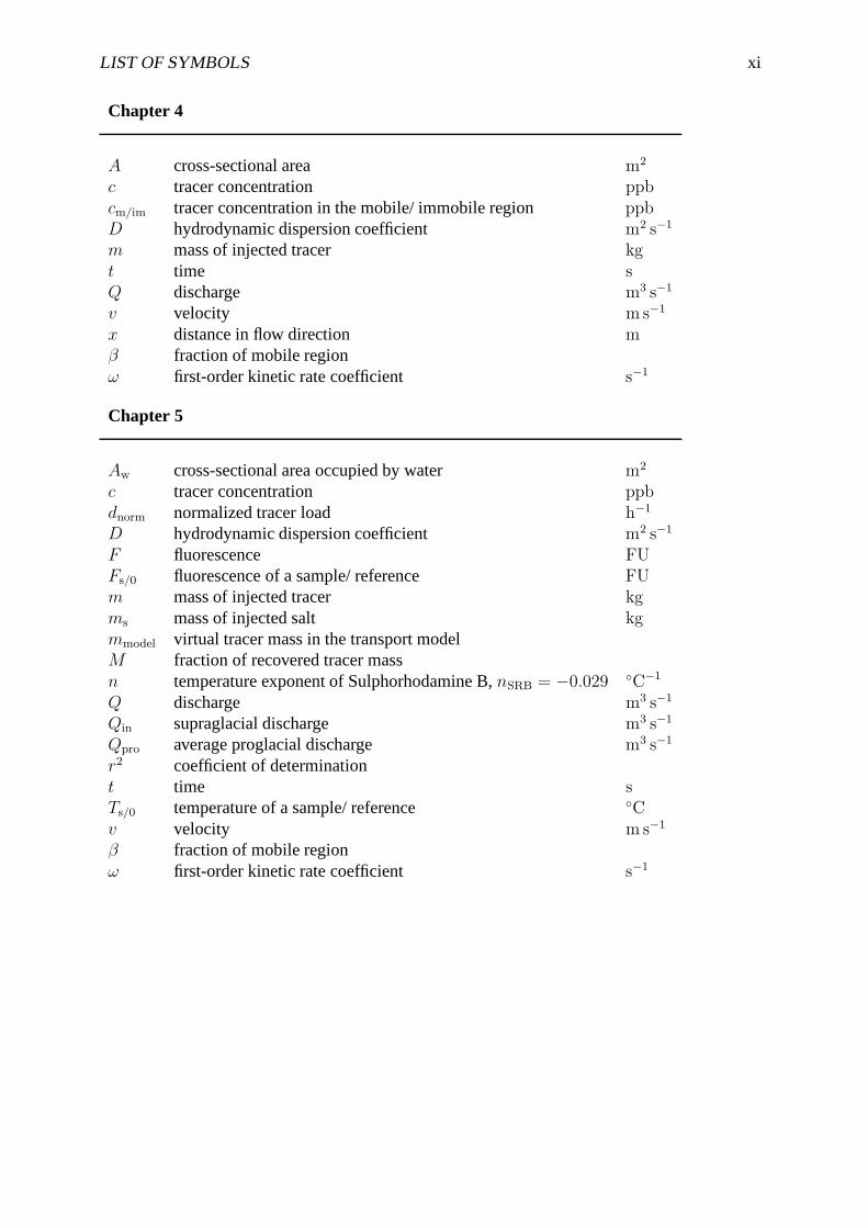
Chapter 5
Aw cross-sectional area occupied by water m2
c tracer concentration ppbdnorm normalized tracer load h−1
D hydrodynamic dispersion coefficient m2 s−1
F fluorescence FUFs/0 fluorescence of a sample/ reference FUm mass of injected tracer kgms mass of injected salt kgmmodel virtual tracer mass in the transport modelM fraction of recovered tracer massn temperature exponent of Sulphorhodamine B, nSRB = −0.029 ◦C−1
Q discharge m3 s−1
Qin supraglacial discharge m3 s−1
Qpro average proglacial discharge m3 s−1
r2 coefficient of determinationt time sTs/0 temperature of a sample/ reference ◦Cv velocity m s−1
β fraction of mobile regionω first-order kinetic rate coefficient s−1

LIST OF SYMBOLS xii
Chapter 6
a, b, c denote arbitrary termsA cross-sectional area m2
Aeff effective cross-sectional area of an inclined moulin m2
Ainc cross-sectional area of an inclined moulin m2
Am/c cross-sectional area related to melting/ closure m2
Amoulin cross-sectional area of the moulin m2
Aw cross-sectional area occupied by water m2
B flow law coefficient Pa−3 s−1ct pressure melting coefficient K J−1 m3
cw specific heat of water J K−1 kg−1
C ratio to which the perimeter is wettedd number of local lossesE energy JEm energy available for melt JEt energy related to a change in pressure melting point Jf friction factor in Equation (6.9)fbottom friction factor of a conduit bottomfcom composite friction factorfi friction factor of an ice-walled conduitFT turbulent resistance parameter s2 m−5
g gravitational acceleration m s−2
h water pressure (expressed in hydraulic head) mh∗ ice-overburden pressure (expressed in hydraulic head) mhi ice thickness mhmax maximum filling height in a moulin mhmoulin water level in the moulin mH total hydraulic potential (expressed in hydraulic head) m∆Hloc local loss of hydraulic potential mi number of equations (subscript)k roughness coefficient in Equation (6.11) m1/3 s−1
kbottom roughness coefficient of a conduit bottom m1/3 s−1
kcom composite roughness coefficient m1/3 s−1
ki roughness coefficient of an ice-walled conduit m1/3 s−1
Lf latent heat of fusion kJ kg−1
n flow law exponentpw water pressure PaQ discharge m3 s−1
Qconduit discharge through main conduit m3 s−1
Qin/out net discharge into/ out of the moulin m3 s−1
Qlow/up lower/ upper limit of discharge variation m3 s−1
Qmax maximum open-channel discharge m3 s−1
Qsub subglacial discharge m3 s−1

LIST OF SYMBOLS xiii
real subscript to denote a real value as opposed to a modeled onerr relative roughnessR radius mRh hydraulic radius mRL/T linear/ turbulent resistance s m−2
RP resistance of a rigid pipe s m−2
RR resistance of a Röthlisberger channel s m−2
Re Reynolds-numbert time sT period of discharge variations dU perimeter mUw wetted perimeter mv mean velocity m s−1
Vm volume produced by melting m3
x distance in flow direction mX, Y denoting left and right hand side of Equation (6.16)z elevation of the glacier bed mzbottom elevation of the moulin bottom mztracer elevation of the tracer in the moulin mα opening angle πγ constant introduced in Equation (6.5), γ = ctcwρw
ε objective functionε infinitesimally small time constant sν kinematic viscosity of water m2 s−1
ξ coefficient of hydraulic head lossξloc coefficient of local head lossΦ angle of inclination ◦
ρw/i density of water/ ice kg m−3
ω angular velocity s−1

LIST OF SYMBOLS xiv
Chapter 7
B body force vector Ncµ constant in eq. 7.6Dm coefficient of molecular diffusion m2 s−1
F transfer function of a black-box systemI input into a black-box systemk turbulent kinetic energy m2 s−2
m, n denoting different time stepsO output from a black-box systemp fluid pressure Pat time sv fluid velocity vector m s−1
v0 inlet velocity m s−1
δt time scale for Reynolds-averaging sε turbulence dissipation rate m2 s−3
µ molecular viscosity Pa sµT turbulent viscosity Pa sρ fluid density kg m−3
τ time sΦ an arbitrary quantityΨ a scalar

xv
Abstract
In this thesis, the water flow through and from Unteraargletscher, an alpine glacier in theBernese Alps, Switzerland, is investigated with particular emphasis on the internal plumbingand its behavior in time.
To quantify water input to the glacial hydrological system during the ablation season 1999,a distributed temperature index melt model including potential clear-sky solar radiation wasapplied to Unteraargletscher. Model parameters were determined by calibrating calculated meltwith ablation measurements. Discharge was measured in the proglacial stream for 18 days untilthe station was destroyed by an outburst flood. Comparison of modeled melt and measureddischarge reveals an imbalance which suggests that water was stored in or beneath the glacierduring this period. The culminating outburst flood presumably released this en- or subglaciallystored water and may be related to a change in the configuration of the glacial drainage systemas inferred from measurements of subglacial water pressure.
The morphology of the drainage system and its diurnal variability were investigated by con-ducting series of tracer tests over a number of discharge cycles during the ablation season 2000.Dye injections into a moulin were repeated at intervals of a few hours and were accompaniedby simultaneous measurements of discharge of supraglacial meltwater draining into the moulinand bulk runoff in the proglacial stream. Records of dye concentration were analyzed using anappropriate transport model. Results of this analysis reveal a large diurnal variability in termsof transit velocity and dispersion coefficients. Furthermore, the obtained velocity-discharge andvelocity-dispersion relationships display pronounced hystereses, thereby inhibiting the use ofconventional evaluation techniques.
A time-dependent and physically-based model of subglacial water flow is used to investigatethe observed variations of transit velocity. It is found that the ability of a Röthlisberger-channelto adjust its size to the prevailing hydraulic conditions contributes to hysteresis of the velocity-discharge relationship. Additionally, the model results further suggest that such hysteresis canbe caused also by retardation of water due to inflow modulation at the junction of a tributarymoulin and a main conduit.
Further, we studied the relation between conduit cross-section and tracer dispersion with nu-merical tracer experiments. The velocity field for steady flow through a given conduit geometryis calculated using a commercial flow solver. Tracer transport is represented by a scalar vol-ume which is advected by the velocity field. Experiments were conducted for several scenariosby varying flow velocity and conduit geometry. Results show that a functional dependence ofdispersion on the hydraulic radius of the conduit exists but it is weak. Further, it is found thatthe dispersion coefficient is strongly affected by changes in roughness. This suggests, that adynamical conduit geometry can account for the observed velocity-dispersion hysteresis, espe-cially, if the evolution of the conduit involves also roughness changes. Additionally, the effect

ABSTRACT xvi
of inflow modulation on tracer dispersion is found to provide an equivalent explanation of theobserved hysteretic behavior.

xvii
Zusammenfassung
In der vorliegenden Abhandlung wird der Wassertransport durch und der Abfluss vom Unter-aargletscher in den Berner Alpen, Schweiz, untersucht. Dabei wird besondere Aufmerksamkeitdem internen Abflusssystem und seiner zeitlichen Entwicklung gewidmet.
Um den Wasserinput in das Gletscherabflusssystem während der Ablationsperiode 1999 zuquantifizieren, wurde ein flächenverteiltes Schmelzmodell auf den Unteraargletscher angewen-det. Dieses Modell basiert auf einem Temperatur-Index Verfahren, das auch die potentielleSolarstrahlung mit einschliesst. Die Parameter des Modells wurden mit einer Kalibrierungder berechneten Schmelze anhand von Ablationsmessungen bestimmt. Der Wasserabfluss imGletscherbach wurde über eine Periode von 18 Tagen aufgezeichnet, bis die Messstation voneiner Flutwelle zerstört wurde. Die Bilanz von berechneter Schmelze und gemessenem Abflussist unausgeglichen, was auf eine Wasserspeicherung während dieser Periode in oder unter demGletscher hinweist. Dieses intra- oder subglazial gespeicherte Wasser wurde vermutlich ineinem anschliessenden Wasserausbruch, der die Flutwelle im Gletscherbach erzeugte, wiederfreigesetzt. Dieser Ausbruch wird mit einer Neukonfigurierung des Gletscherabflusssystems,die von Messungen des subglazialen Wasserdrucks abgeleitet wurde, in Verbindung gebracht.
Die Morphologie des Abflusssystems und dessen tageszeitliche Variabilität wurde mit Serienvon Tracerversuchen untersucht, die über einige Abflusstageszyklen während der Ablation-speriode 2000 durchgeführt wurden. Dabei wurden die Tracereingaben in eine Gletscher-mühle in Intervallen von wenigen Stunden wiederholt. Gleichzeitig wurde der Abflussim supraglazialen Bach, der in die Mühle entwässert, ebenso wie der Gesamtabfluss improglazialen Fluss gemessen. Die erhaltenen Datenreihen der Tracerkonzentrationen wur-den mit einem geeigneten Transportmodell ausgewertet. Die Resultate dieser Analyse weiseneinen ausgeprägten Tagesgang der Abstandsgeschwindigkeiten und der Dispersionskoeffizien-ten auf. Die daraus abgeleiteten Geschwindigkeits-Abfluss- und Geschwindigkeits-Disper-sions-Beziehungen zeigen jeweils eine deutliche Hysterese. Dieser Umstand verhinderte eineweitere Auswertung mittels konventioneller Verfahren.
Ein zeitabhängiges und physikalisch basiertes Modell subglazialer Abflussprozesse wurdeeingesetzt, um die beobachteten Variationen der Abstandsgeschwindigkeiten zu untersuchen.Es ergab sich, dass die Eigenschaft eines Röthlisberger-Kanals, seine Grösse an dievorherrschenden hydraulischen Bedingungen anzupassen, zur Hysterese der Geschwindigkeits-Abfluss-Beziehung beiträgt. Zudem geben die Modellergebnisse zu erkennen, dass eine solcheHysterese ebenfalls durch eine Regulierung des Zuflusses aus einer Gletschermühle in einenHauptkanal verursacht werden kann.
Des weiteren wurde die Beziehung zwischen dem Kanalquerschnitt und der Tracer-Dispersionmit numerischen Tracerexperimenten untersucht. Dabei wurde zuerst mit einem kommerziellenProgramm das stationäre Geschwindigkeitsfeld durch eine gegebene Kanalgeometrie berech-net. Der Tracertransport wurde daraufhin simuliert mittels einem Skalarvolumen, das mit

ZUSAMMENFASSUNG xviii
diesem Geschwindigkeitsfeld advektiert wird. Experimente für mehrere Szenarien wurdendurchgeführt, indem die Fliessgeschwindigkeit oder die Kanalgeometrie geändert wurden.Die Ergebnisse zeigen, dass zwar ein funktionaler Zusammenhang zwischen der Disper-sion und dem hydraulischen Radius des Kanals besteht, dieser aber schwach ist. Ausser-dem stellte sich heraus, dass der Dispersionskoeffizient stark von Rauhigkeitsänderungen bee-influsst wird. Diese Ergebnisse deuten an, dass eine dynamische Kanalgeometrie für diebeobachtete Geschwindigkeits-Dispersions Hysterese verantwortlich gemacht werden kann,besonders, wenn die Entwicklung des Kanals mit einer Rauhigkeitsänderung einhergeht. Zu-dem wurde gezeigt, dass eine Zufluss-Regulierung einen ähnlichen Effekt auf die Tracerdis-persion hat und somit eine äquivalente Erklärungsmöglichkeit für die beobachtete Hysteresebietet.

Chapter 1
Introduction
Zuletzt wollten zwei oder drei stille Gäste sogar einen Zeitraum grimmiger Kältezu Hülfe rufen und aus den höchsten Gebirgszügen, auf weit ins Land hinausge-senkten Gletschern, gleichsam Rutschwege für schwerste Ursteinmassen bereitet,und diese auf glatter Bahn, fern und ferner hinausgeschoben im Geiste sehen. Siesollten sich, bei eintretender Epoche des Auftauens, niedersenken und für ewig infremdem Boden liegen bleiben. Auch sollte sodann durch schwimmendes Treibeisder Transport ungeheurer Felsblöcke von Norden her möglich werden. Diese gutenLeute konnten jedoch mit ihrer etwas kühlen Betrachtung nicht durchdringen. Manhielt es ungleich naturgemäßer die Erschaffung einer Welt mit kolossalem Krachenund Heben, mit wildem Toben und feurigem Schleudern vorgehen zu lassen.
J. W. Goethe, Wilhelm Meisters Wanderjahre, 1829
1.1 Significance of glacial hydrology
1.1.1 Glacier dynamics
An early intimation that erratic boulders might be indicative of a major climate change camefrom the poet Goethe. The possibility of such boulders being of glacial origin was a pioneeringthought at the time when it was mentioned in his novel Wilhelm Meisters Wanderjahre. Goethequite reasonably believed that a vast amount of ice was required to explain the observed distribu-tion of boulders by glacial transport and he inferred the existence of a considerably colder periodin the past (Goethe, 1829). Today, there is little doubt about the existence of such ice-ages butthe current discussion in the context of global climate change concentrates on the mechanismof ice sheet collapse by sudden discharges of ice at the termination of a glacial period. Similarchanges between states of rapid and slow motion of ice-masses is today observed as switchingon and off of ice streams (e.g. the Siple Coast ice streams in Antarctica), as pulsating flow ofsurging glaciers (e.g. Variegated Glacier, Alaska) and as short term “speed-up events” of alpineglaciers.
Variations in glacier motion are to a great extent associated with changes in conditions at theinterface between ice and the underlying bed (Paterson, 1994). It is generally accepted that the
1

CHAPTER 1. INTRODUCTION 2
subglacial hydrological system has a strong influence on basal conditions as high subglacialwater pressures lead to a decoupling of the glacier from its bed thereby promoting basal slid-ing (Boulton et al., 1974; Bindschadler, 1983; Iken et al., 1983; Iken and Bindschadler, 1986;Kamb and Engelhardt, 1987; Hooke et al., 1989). At the same time high subglacial water pres-sures can also cause the sediment comprising the bed to weaken enabling sediment deformation(Boulton and Jones, 1979; Boulton and Hindmarsh, 1987; Iverson et al., 1995; Fischer et al.,1999; Fischer and Clarke, 2001; Fischer et al., 2001).
Elevated basal water pressures result from the inability of the subglacial drainage system todischarge water at the same rate as it is supplied to the system from the glacier surface. Thissituation can arise at the beginning of the ablation season when rapid melting of the wintersnowpack causes a sudden influx of large amounts of meltwater to an inefficient winter drainagesystem.
In response to high subglacial water pressures, hydraulic and mechanical instabilities can resultwhich then lead to a reorganization of the subglacial drainage system (e.g. Gordon et al., 1998;Stone and Clarke, 1996) or periods of enhanced glacier motion (e.g. Iken et al., 1983; Kamb andEngelhardt, 1987; Kavanaugh and Clarke, 2001). These velocity increases are often accompa-nied by anomalous vertical surface velocities of the order of 10 cm d−1 (Iken et al., 1983; Mairet al., 2001). Surface uplifts were initially interpreted to result from water storage at the bed.Measurements of vertical and horizontal strain suggest that temporal variations in the strain-rateregime may also contribute to the observed surface uplifts (Gudmundsson, 1996).
The subsequent establishment of stable hydraulic and mechanical conditions at the glacier bedis often marked by a sudden release of the subglacially backed-up water and an increasedsuspended-sediment flux (e.g. Anderson et al., 1999; Barrett and Collins, 1997; Collins, 1998;Humphrey et al., 1986).
The same processes are used to explain glacier surging (Raymond, 1987; Kamb et al., 1985;Humphrey et al., 1986; Kamb, 1987; Humphrey and Raymond, 1994; Björnsson, 1998). For agiven constellation of bed roughness, ice rheology, glacier geometry and hydraulic conditions,an inefficient drainage system may be stable enough against water pressure perturbations. Inthis way, high subglacial water pressures and thereby increased basal motion can be maintainedover some time. The surge is terminated when the subglacial drainage morphology switches toa hydraulically more efficient structure.
1.1.2 Glacial discharge
Besides its glacier-dynamical aspects, the internal plumbing of a glacier is also of significancefor hydrological purposes. In many regions, glaciers provide substantial water supply to thesurrounding lowlands which benefit notably from the compensating effect of glaciers, releas-ing meltwater typically during periods of precipitation deficit (Röthlisberger and Lang, 1987).However, regions in vicinity to glaciers are also vulnerable to floods caused by sudden outburstsof stored water from the glacier itself or from ice- or moraine-dammed lakes. Therefore, accu-rate estimates of the volume and timing of glacial runoff is required for water resource and riskmanagement purposes. Such tasks include flood control and prediction, efficient water manage-ment and design and operation of hydroelectric facilities and protective installations. Specialconsideration is given to these issues as most glaciers world-wide decrease in volume due toglobal climate change (e.g. WGMS, 1999).

CHAPTER 1. INTRODUCTION 3
Assessing a possible future evolution of glacial water resources and risks related to glacialdischarge requires models which describe the relevant processes. A variety of methods to cal-culate discharge from glaciers has been developed (e.g. Fountain and Tangborn, 1985; Hock,1998). Efforts have been undertaken to simulate the melt process accurately but the water trans-fer through the glacier is mostly represented by a black-box model based on a linear reservoirapproach (e.g. Mader and Kaser, 1994; Braun and Aellen, 1990; Baker et al., 1982) therebyneglecting the dynamic nature of a glacial drainage system.
Another shortcoming of a black-box approach is that it cannot provide meaningful insight intothe system when detailed or distributed information is required. For instance, subglacial waterpressures are of particular concern where water is tapped from under the glacier for hydropowerpurposes (e.g. Vivian and Bocquet, 1973; Hagen et al., 1983; Jansson et al., 1996) or wherewater should be drained from mines underneath a glacier (Melvold et al., 2002).
1.2 Techniques of investigation
Because of the inaccessibility of the bed, hydraulic conditions and processes prevailing beneathglaciers are difficult to study and therefore our present understanding of subglacial hydrologyis incomplete. The character of the subglacial drainage system and its physical parameters haveto be deduced from experimental techniques in conjunction with theoretical considerations.Experiments using tracer methods have made a major contribution to the understanding of waterflow beneath glaciers (Röthlisberger and Lang, 1987) and are thus considered to provide the bestdata for determining the structure of subglacial drainage systems (Hooke, 1989). The relativelysimple procedures required mean that tracer techniques are ideal for temporally intensive andspatially extensive investigations (Nienow, 1993). Tracer tests provide general characteristicsof the water flow path, the rate at which water flows through the glacier and the extent to whichthe water is delayed during its passage through the system (e.g. Behrens and others, 1975).
Tracer techniques have been used to elucidate the nature and the seasonal evolution of thedrainage system beneath a number of glaciers including Haut Glacier d’Arolla (Nienow, 1993;Nienow et al., 1996c, 1998) and Storglaciären (Hooke et al., 1988; Seaberg et al., 1988; Hockand Hooke, 1993; Kohler, 1995). Repeated dye tracing experiments at Haut Glacier d’Arollashowed that both the transit velocity and the degree of tracer dispersion changed over the courseof the summer suggesting that the hydrological system changed from an initial inefficient con-figuration to a more efficient one over large parts of the glacier bed.
Seaberg et al. (1988), Fountain (1993) and Kohler (1995) developed conceptual models of sub-glacial drainage to infer hydraulic conditions from tracer tests. However, the interpretation ofsuch tracer tests using a physically based model of subglacial drainage has not been attemptedto date. Such a model would enable the identification of the governing processes and the deter-mination of the contribution of individual mechanisms. As such, the information yield of tracertests would be significantly enlarged.
1.3 Study area: Unteraargletscher
This study was performed on Unteraargletscher, a temperate valley glacier situated in theBernese Alps, Switzerland (Fig. 1.1). Already in the first half of the 19th century, Unteraar-

CHAPTER 1. INTRODUCTION 4
0320
2600
0300
2800
2600
3000
2
0 1 2 3
km
N
0082
000
3
2600
0082
2400
+ meteo station
gauging station
Unteraargletscher
SWITZERLAND
Lauteraar
Strahlegg
Unteraar
28003000
borehole 1999
tracer injection 2000
200
Finste
raar
SAC Lauteraarhut
Figure 1.1: Map of Unteraargletscher showing the location of the Lauteraarhut and the sitesof various glaciological, meteorological and hydrological measurements conducted during thefield-campaigns 1999 and 2000. Inset shows the location of the study area in the Bernese Alps,Switzerland.
gletscher was object of scientific investigations by Franz Josef Hugi and Louis Agassiz (Hugi,1830, 1842; Agassiz, 1840, 1847). Their pioneering work contributed substantially to ourpresent understanding of glaciers. Since the 1920s systematic measurements of changes in sur-face elevation and displacement have been conducted (Flotron, 1924 to date). A comprehensivelist of references to work related to Unteraargletscher can be found in Zumbühl and Holzhauser(1988, 1990). Today, Unteraargletscher belongs to the most comprehensively studied glaciersin the Alps.
Unteraargletscher is the common tongue of the two tributaries Lauteraar- and Finsteraar-gletscher (Fig. 1.1). From the confluence zone at ∼2400 m above sea level (a.s.l.), Unteraar-gletscher extends about 6 km eastwards with a mean width of 1 km and a slope of approximately4◦. The entire system of glaciers covers an area of 26 km2. The present terminus, ∼1.5 km fromLake Grimsel, is at an elevation of 1950 m a.s.l, and the headwalls of the accumulation basinsare surrounded by peaks up to 4274 m a.s.l. Despite the lack of detailed mass balance measure-ments, the present equilibrium-line altitude is estimated at ∼2800 m a.s.l. based on a compar-ison with other glaciers in the area and on an analysis of aerial photographs (Gudmundsson,1994).
A prominent feature of Unteraargletscher is the large ice-cored medial moraine which is formedby the convergence of the lateral moraines of Lauteraar- and Finsteraargletscher. The debriscover is typically 5 to 15 cm thick. At the confluence zone the medial moraine is between 10 and20 m high and ∼100 m wide. With distance downglacier it grows to a maximum height of 50 mand width of 300 m before it gradually spreads out and merges with the marginal morainic debris

CHAPTER 1. INTRODUCTION 5
in the terminus region. Smaller medial moraines on the southern side of Unteraargletscher arethe result of Finsteraargletscher being fed by Strahlegggletscher and a number of smaller trib-utaries. In contrast, there are no tributaries that feed large amounts of ice to Lauteraargletscherand, thus, the northern side of Unteraargletscher is nearly debris-free.
For simplicity we refer in the remainder of this study to the entire system of glaciers (Fig. 1.1)as “Unteraargletscher”. The catchment area of Unteraargletscher is embedded in the centralmassif of the Alps, namely the Aare-massif (Labhart, 1992). This formation belongs to thevarascic basement and consists of old crystalline gneiss and Aare-granite .
The bedrock topography of Unteraargletscher has been mapped by seismic reflection and radio-echo soundings (Knecht and Süsstrunk, 1952; Sambeth and Frey, 1987b; Funk et al., 1994;Gudmundsson, 1994; Bauder, 2001) (Fig. 1.2a). Two seismic reflectors at different depth havebeen identified, where the upper one represents the true glacier bed and the lower one the sur-face of the underlying bedrock. The intervening layer consists of unconsolidated sedimentarymaterial (Sambeth and Frey, 1987a). From the systematic thinning of the sediment layer inup-glacier direction and its final disappearance at the confluence it has been inferred that atransition from bed erosion to sedimentation occurs in down-glacier direction (Gudmundsson,1994). The glacier bed of Unteraargletscher is U-shaped in transverse direction and is onlyweakly inclined down-glacier from the confluence area. Maximum ice-thickness of more than400 m is observed up-glacier of the junction on both tributaries, Lauteraargletscher and Finster-aargletscher (Fig. 1.2b). From there, the ice-body thins out but at a distance of 1.5 km from theterminus it is still ∼200 m thick (Funk et al., 1994; Bauder, 2001).
1.4 Objectives
The main goals of this thesis are to gain a better understanding of subglacial drainage, to identifythe governing processes and to determine their effects on hydraulic conditions. In detail, theseobjectives were achieved by:
• studying the water balance of Unteraargletscher prior to a release event with regard topossible subglacial water storage.
• conducting tracer injections in quick succession over a range of different discharges toinvestigate the morphology of the drainage system and its diurnal variability.
• a careful analysis of the data obtained from tracer tests and accompanying discharge mea-surements to determine transport parameters.
• developing a physically based, numerical model of subglacial drainage to interpret theexperimentally observed variations of transit velocity.
• performing numerical tracer experiments to investigate mechanisms of tracer dispersionand thereby elucidating the behavior of dispersion observed in the experiments.

CHAPTER 1. INTRODUCTION 6
657 658 659 660 661 662 663Easting [km]
156
157
158
159
Nor
thin
g [k
m]
2300
2300 22002200
21002100
2100
20002000
2000
2000 1900
2100
2300
2300
21002100
21002200
2200
22002200
657 658 659 660 661 662 663Easting [km]
156
157
158
159
Nor
thin
g [k
m]
100
100
100
100
300
300
300200
200
200
200
200
300
100 100
100
400
a
b
Figure 1.2: (a) Basal topography and (b) ice-thickness of Unteraargletscher in 1996. Shadedareas denote the surrounding topography which was used for the interpolation (Bauder, 2001).

CHAPTER 1. INTRODUCTION 7
glacier dynamics
glacial discharge
process understanding (Chapter 2)
synthesis (Chapter 8)
this thesis:
review
water balance
(Chapter 3)
tracer tests (Chapter 4 and
Chapter 5)
numerical modeling
velocity variations (Chapter 6)
dispersion variations (Chapter 7)
interpretation
observedbehavior
significant for
studied by
water transfer through a glacier
Figure 1.3: The structure of this thesis.
1.5 Structure of the thesis
Figure 1.3 sketches the organization of this thesis. Chapter 2 introduces the processes involvedin glacier melt and discharge and gives a review of previous work. As such, it provides thebackground knowledge on which this thesis is based. In Chapter 3, the possibility that waterwas stored in Unteraargletscher and contributed to a flood event is investigated by balancingwater input and output. For this reason, the water input was determined using a melt modeland compared to measured discharge. The content of this chapter has recently been publishedin Nordic Hydrology (Schuler et al., 2002). Chapter 4 introduces the principles of tracer tests.Further, models of tracer transport are presented which provide the basis for the evaluation

CHAPTER 1. INTRODUCTION 8
of the experimental part of this study. Based on theoretical considerations made in Chapter 2and Chapter 4, appropriately designed tracer experiments were performed at Unteraargletscher.Chapter 5 describes the strategy of data acquisition and subsequent analysis. The implicationof the results for subglacial plumbing are discussed. In Chapter 6, a physically based model ofsubglacial conduit drainage is developed to investigate mechanisms accounting for the observedvariation of transit velocity. Similarly, a numerical model of tracer transport is used in Chapter 7to study the observed behavior of tracer dispersion. The results obtained in this chapter formthe substance of a paper which is accepted for publication in Annals of Glaciology (Schuler andFischer, 2002). Finally, the thesis is concluded by Chapter 8 discussing the main findings of theprevious chapters with regard to conclusions drawn from other studies.
Chapter 2
Glacial hydrology: a process review
Most of the runoff from the surface of an alpine glacier disappears into the glacier and emergesfrom under the terminus in one or a few large streams. The interior of the glacier is virtuallyinaccessible (Röthlisberger and Lang, 1987) and therefore observations of the internal plumbingare difficult to obtain (Hooke, 1989). Hence, the character of the subsurface drainage systemhas to be deduced from theoretical consideration and indirect experimental techniques such astracer tests or borehole water level monitoring. In this section, the findings of previous studies ofglacial water production and routing are summarized and the significance of glacial hydrologyfor the motion of glaciers and water resource management are illustrated.
2.1 Runoff generation at the surface
For temperate glaciers, the most important contribution to bulk runoff originates at the glaciersurface (e.g. Paterson, 1994; Röthlisberger and Lang, 1987). This water is derived from meltingof snow, firn and ice, from rainfall or from inflow of extraglacial water. Additional contributionsare provided by meltwater produced internally in the glacier by dissipation of energy related tothe flow of ice or water and by basal meltwater caused by the geothermal heat flux. Theseinternal and basal contributions play a minor role in alpine glacial hydrology since they are onthe order of only 10−2 m a−1 while surface melt rates range from 0.1 to 10 m a−1 (Röthlisbergerand Lang, 1987). A basic understanding of the melt process at the surface is therefore essentialfor a comprehensive characterization of runoff which is drained through or beneath a glacier.
2.1.1 Surface energy balance
The balance of all energy fluxes from or towards a glacier surface of unit area is given by
QN + QH + QL + QG + QR + QM = 0
where QN is the net radiation, QH is the sensible heat flux, QL is the latent heat flux related tophase changes, QG is the heat exchange with the ground, QR is the heat flux supplied by rainand QM is the flux of latent energy available for melt. By convention, energy fluxes directedtowards the surface are denoted by a positive sign while those away from the surface carry anegative sign.
9

CHAPTER 2. GLACIAL HYDROLOGY: A PROCESS REVIEW 10
Net radiation (QN )
The net radiation is the difference between radiation directed to or away from the consideredsurface (Kondratyev, 1965). It can be further subdivided into a shortwave component (rangingfrom 0.15 to 4 µm) which is predominantly of solar origin and into a longwave part of mainlyterrestrial origin (4 to 120 µm). The global radiation (incoming shortwave radiation) is subjectto considerable variability in space and time due to effects of slope, aspect and effective hori-zon. The reflected part of global radiation is controlled by the shortwave albedo of the surface,therefore increasing the variability of QN (Kondratyev, 1965). Thermal emission from the loweratmosphere and the considered surface contribute to QN in the longwave spectrum.
Sensible and latent heat (QH , QL)
The fluxes of sensible and latent energy are proportional to the vertical gradients of air tem-perature and specific humidity. The exchange of energy in both cases is driven by turbulencein the lower atmosphere. Hence the expressions for both turbulent fluxes are analogous. Themagnitude of turbulence depends on wind speed, surface roughness and atmospheric stability(Morris, 1989).
Rain heat flux QR and ground heat flux QG
The energy flux provided by rainfall onto the glacier is determined by precipitation intensity andrain temperature. Vertical exchange of energy between the surface and the underlying glacier iceoccurs in winter mainly by heat conduction. Otherwise, percolation of surface meltwater into apermeable medium (snow, firn) and refreezing of that water at a depth where the temperature isbelow 0◦C is the most efficient process to warm up the snow (e.g. Paterson, 1994). However,the surface temperature cannot rise above 0◦C.
Heat available for melting QM
A necessary condition to start meltwater production is a glacier surface at the melting point.Once this condition is met and the budget of all other components provides a surplus of energy,the residual flux QM is used for melting.
2.1.2 Importance of energy fluxes
The assumption of the surface of a temperate glacier being at the melting point is appropriate formost alpine glaciers during the ablation season. In this case some terms of the energy balanceequation can be neglected. At a temperate glacier surface, QG vanishes except for occasionalperiods of nocturnal freezing (Paterson, 1994) and Röthlisberger and Lang (1987) demonstratedthat QR is significant only for extreme rainfall events and only on a short time-scale. As opposedto a soil surface or to a surface covered by vegetation, the low temperature of a glacier surfacefavors the formation of atmospheric stable conditions thereby supressing turbulence. Thus, theturbulent fluxes generally play a minor role for snow and ice melt compared to the flux of netradiation (e.g. Lang and Schönbächler, 1967; Lang et al., 1977). Nevertheless, highest melt

CHAPTER 2. GLACIAL HYDROLOGY: A PROCESS REVIEW 11
rates coincide with high values of the turbulent fluxes (Hay and Fitzharris, 1988) and the flux oflatent energy can be of importance for the short-term variations of melt rates (Lang, 1981).Ohmura (2001) presented an extensive review of energy balance measurements on glaciersand lists the components in their order of significance for meltwater generation. This paperunderlines the dominating role of net radiation which the author examined in more detail. Onaverage, longwave incoming radiation is by far the largest energy source, followed by absorbedglobal radiation. From this follows the pronounced temporal and spatial variability of meltwhich is characteristic for runoff generation on glaciers. Since longwave incoming radiationand sensible heat flux components are very closely related to air temperature (Lang and Braun,1990), the course of melt water generation is to a large extent explained by the variation ofair temperature (Ohmura, 2001). The resulting pattern of the melt distribution is modulated bythe variability of the absorbed global radiation. The amount of incoming shortwave radiationdepends on zenith angle, cloudiness and topography whereas the absorption is controlled bysurface properties such as albedo and roughness. Albedo of a glacier surface experiences drasticvariations which may range from 0.1 for dirty ice to more than 0.9 for fresh snow (Warren,1982). Many authors reported how snowfall during the ablation season affected meltwatergeneration (e.g. Hoinkes and Rudolph, 1962; Tronov, 1962). Lang (1966) estimated a 27%reduction of monthly runoff from Hintereisferner due to one snowfall in July.
To summarize, the melt water production is characterized by an enormous temporal variabilityon a seasonal as well as diurnal time scale which is a consequence of the governing influenceof air temperature and absorbed global radiation. Due to its high albedo, the presence of a snowcover on the glacier and the retreat of the snow line during the ablation season introduces furthercomplexity in the temporal and spatial pattern of melt.
Ablation areaAccumulation area
bergschrund
snow
firn snowmeltpercolation
transientsnowline
ice
ice - bedrockinterface
base? englacial and basal moraine
subglacialconduits
firnlinecrevasses
moulin
watersaturated
zone supraglacialice meltwater
percolation proglacialmeltstream
flow
englacialconduits
basalarterialtunnel
subglacialcavities
portal
liquid precipitation
impermeable
groundwater
subglacial pipes
channels
Figure 2.1: Schematic diagram of supraglacial, englacial and subglacial drainage pathways ofa temperate glacier (after Röthlisberger and Lang (1987), taken from Collins (1988)).
2.2 Water flow through the glacier
Drainage from an alpine glacier takes place in a complex system consisting of numerous el-ements. Generated at the glacier surface by melting or rainfall, water percolates through the

CHAPTER 2. GLACIAL HYDROLOGY: A PROCESS REVIEW 12
snow or firn layer in the accumulation zone or where a transient snow cover exists. In the abla-tion zone where the winter snow cover has disappeared, water flows on bare ice, channelised insupraglacial streams. Crevasses and moulins provide access to the interior of the glacier wherethe water continues to the glacier bed flowing in conduits, through a network of interconnectedcavities or in a permeable basal sediment layer (Röthlisberger and Lang, 1987; Fountain andWalder, 1998).
Figure 2.1 sketches the structure of the principal drainage pathways, their location in the glacierand probable interactions between them. Accordingly, glacier drainage is subdivided into threemain parts:
• the flow within the snow-firn layer and along the ice surface
• the transfer to and the passage through the interior of the glacier and
• the subglacial drainage pathways.
For further details of glacial hydrology beyond the discussion presented below, I refer to moreextensive reviews (Röthlisberger and Lang, 1987; Hooke, 1989) and the more recently pub-lished work of Fountain and Walder (1998) and Hubbard and Nienow (1997).
2.2.1 Firn and supraglacial hydrology
At the onset of the melt period, the glacier is typically covered by a winter snow cover. Whereyearly mass gain exceeds mass loss, the snow is transformed into firn, a transitional materialin the metamorphism of snow to ice. The hydrological behavior of the snow and firn layers iscomparable to a porous aquifer in soil hydrology (Meier, 1973). Gravity drives the percolationof water through unsaturated snow or firn (Colbeck and Davidson, 1973; Ambach et al., 1981)down to a zone of substantially lower permeability where a saturated layer builds up (Ambachet al., 1978; Behrens et al., 1979). Water level monitoring, pumping tests and dye tracer exper-iments (Schommer, 1977; Ambach and Eisner, 1979; Oerter and Moser, 1982; Fountain, 1989;Schneider, 1999, 2001) reveal that the passage of water through firn is considerably delayeddue to a low hydraulic conductivity on the order of 10−5 m s−1. Substantial volumes of waterare temporarily stored within the firn layer. As a consequence, diurnal variations in melt waterrunoff are substantially dampened during its passage through the firn (Schneider, 2001).
The firn aquifer is discharged by outflow on the ice surface at the firn line, by drainage intocrevasses underneath (Schneider, 2001) or by seepage through the glacier ice through inter-granular veins (Röthlisberger and Lang, 1987). The latter process was discussed by Lliboutry(1964), Shreve (1972) and Nye and Frank (1973) but observations reveal that the quantity ofintergranuler drainage is probably negligible (Raymond and Harrison, 1975; Lliboutry, 1971,1996).
In contrast to the firn layer, the bare ice surface has hardly any retention capacity to delay theinput of water into the body of the glacier. Penetration of shortwave solar radiation enlarges in-tergranular veins (Lliboutry, 1971; Brandt and Warren, 1993), but substitution of melted surfaceice by ice emerging from the interior of the glacier disables the formation of a deeply weatheredcrust. Hence, the ice surface remains relatively impermeable (Lliboutry, 1996) and water flowsin supraglacial channels that disappear into the glacier (Stenborg, 1973). Large surface streamsflowing as far as to the margins or the glacier terminus are only rarely observed (Röthlisbergerand Lang, 1987).

CHAPTER 2. GLACIAL HYDROLOGY: A PROCESS REVIEW 13
2.2.2 Englacial passageways
As mentioned above, several authors considered a general but weak permeability of glacier icevia intergranular veins (Lliboutry, 1964; Shreve, 1972; Nye and Frank, 1973). Shreve (1972) ar-gued that the release of potential energy in the water flowing through such veins would enlargethem to pipes. The visco-plastic property of the surrounding ice would tend to contract suchpipes. By applying a balance of ice-overburden pressure and water pressure, Shreve (1972)described the behavior of such pipes. If two flow paths of different size were competing forthe same discharge, the larger passage would grow at the expense of the smaller one. Röth-lisberger (1972) obtained the same conclusion by balancing closure rate and melt rate. Hence,the englacial conduit system should form an upward branching arborescent network, with trib-utaries joining into larger passages (Fig. 2.2). There is little doubt on the existence of largerenglacial passageways (Raymond and Harrison, 1975; Pohjola, 1994), even though the processinitiating their development is not completely understood.
Flow into crevasses and moulins contributes to a much larger extent to the transfer of meltwa-ter to the interior of the glacier than intergranular seepage does. Whereas drainage of waterto crevasses from underneath the firn layer is inferred from observations of firn water level(Schommer, 1977; Oerter and Moser, 1982; Schneider, 1999, 2001), it is obvious in the abla-tion zone (Röthlisberger and Lang, 1987). Crevasses are tensional fractures in the ice capturingsupraglacial water when they cut across the surface drainage (Hooke, 1989). Within the ice,the crevasse may intersect englacial passages through which the water drains further into theglacier, thereby enlarging the englacial conduits rapidly. Otherwise, if none of such passages isintersected by the crevasse or if their capacity to drain the water is not sufficient, the crevassewill begin to fill. In this case, the higher density of water compared with ice may promote thedownwards propagation of a water filled crack. Robin (1974) and Weertman (1974) proposedhydro-fracturing as the mechanism facilitating inflow of surface water to the glacier bed. Hooke(1984) argued that descending englacial conduits larger than 4 mm in diameter, experience ratesof wall melting in excess of creep closure rates. At a given discharge, the water pressure woulddrop and finally open channel flow would occur. Then, melting would take place at the bottomand thereby causing the conduit to cut gradually downwards.
Moulins are sink holes in the glacier surface (Röthlisberger and Lang, 1987). Their formationis attributed to the establishment of an efficient drainage mechanism starting from a preferentialflow path such as fractures and crevasses. Descends into such moulins (Reynaud, 1987) andmapping structures of ancient moulins as they are exposed at the glacier surface (Holmlund,1988) revealed that they steeply plunge down into the glacier at least in the uppermost (ac-cessible) few decameters. It remains still unclear whether water draining from the bottom ofmoulins continues to descend more or less vertically to the glacier bed (Hooke, 1984). Fromthe difference between the cable length and the pressure reading of a pressure transducer whichwas lowered down a moulin at White glacier, Iken (1972) inferred a gradually decreasing slopewith increasing depth of the moulin. From theoretical considerations it was also argued that thelower part of moulins should be tilted down-glacier (Shreve, 1972) or even up-glacier (Röth-lisberger and Lang, 1987). However, even though their plumbing is not fully understood, it isevident that such englacial drainage structures facilitate rapid transfer of surface water to theglacier bed.

CHAPTER 2. GLACIAL HYDROLOGY: A PROCESS REVIEW 14
Figure 2.2: Hypothetical network of arborescent englacial channels. Flow direction is in generalperpendicular to contours of fluid potential (dotted lines), (after Shreve, 1985).
2.2.3 Subglacial hydrology
Alpine glaciers are typically drained by outflow streams emerging from underneath the glacierterminus discharging turbid water (the so called glacial milk). Since the bulk of the runoff isderived from clear surface meltwater, it is obvious that during its passage at least some of thewater must have experienced contact with sediments at the glacier bed. Another evidence ofhydraulic connections between the glacier surface and the bed was first reported by Mathews(1964) who measured diurnal variations of water pressure at the bed of South Leduc Glacierin response to a diurnally varying meltwater production. Numerous studies following differ-ent approaches identified different subglacial flow systems. Dye tracer experiments (Ambachet al., 1972; Lang et al., 1979; Burkimsher, 1983; Brugman, 1986; Fountain, 1993; Nienowet al., 1998; Hock et al., 1999), investigations of the chemical and isotopic composition ofbulk discharge (Behrens et al., 1971; Collins, 1979; Oerter et al., 1980; Tranter et al., 1996)as well as borehole water level monitoring (Hodge, 1979; Hantz and Lliboutry, 1983; Iken andBindschadler, 1986; Stone and Clarke, 1993; Fountain, 1994; Hubbard et al., 1995; Gordonet al., 1998) suggest the existence of several distinct systems. Distinctions between “fast andslow”, “low and high resistive” or “arborescent and non-arborescent” systems have been madeto categorize subglacial drainage systems. However, these properties can be derived from thegeometry of the system. Therefore, in this thesis, we use the geometry as a criterion and distin-guish between channelised and distributed drainage systems. Weertman (1972) stated that bothtypes of flow may occur side by side, with the surface-derived water showing a preference forchannel flow.
Channelised systems
Once a large englacial conduit reaches the glacier bed it seems implausible that it would dis-appear. Thus, the arborescent tunnel network is likely to continue along the ice-bed interfacetowards the glacier terminus (Shreve, 1972; Röthlisberger, 1972). Further, at the transition froma englacial to a subglacial conduit, the channel properties should remain unaltered since theprinciple of melt enlargement versus creep closure holds unconditionally (Röthlisberger andLang, 1987). However, specific conditions of the glacier bed have to be taken into accountsince they affect both, the motion of water and of ice. The impact on subglacial channel charac-teristics of various factors such as consistence and roughness of the bed, cross-sectional conduitgeometry and properties of basal ice was discussed in detail by several authors proposing differ-

CHAPTER 2. GLACIAL HYDROLOGY: A PROCESS REVIEW 15
ent channel types (Röthlisberger, 1972; Nye, 1973; Hooke, 1984; Hooke et al., 1990; Lliboutry,1983; Walder and Fowler, 1994) (see Fig. 2.3).
Subglacial conduits as described in the theory of Röthlisberger (1972) are commonly referredto as “Röthlisberger-Channels” or “R-Channels”. To compute water pressures in a subglacialchannel, Röthlisberger (1972) and Iken and Bindschadler (1986) assumed a semi-circular cross-section but model results consistently underestimated measured water pressures. Therefore,they had to assume an enhanced tunnel closure rate to achieve agreement between modeledand measured water pressures. Lliboutry (1983, 1996) justified an increased deformation ofbasal ice by enhanced closure rates on the upstream-side of bed obstacles as well as by materialproperties of basal ice. Hooke (1984) and Hooke et al. (1990) argued that the drag on thebed would prevent a semi-circular tunnel to maintain its shape while closing. Thus, its cross-sectional shape should be broad and low instead. Cutler’s (1998) finite element modeling ofthe evolution of subglacial tunnels due to varying water input supports the assumption of abroad and low conduit shape. Sometimes, such a channel is also referred to as “H-channel”(“Hooke-Channel”, in analogy to “Röthlisberger-Channel”) even though the underlying idea isa modification of the Röthlisberger theory rather than an independent one.
Nye (1973) suggested continuous subglacial waterways as channels incised into the bed. Theirhydraulics were described in detail by Weertman (1972). Studies of recently deglaciatedbedrock surfaces provide evidence for the existence of such “Nye-Channels” (Walder and Hal-let, 1979; Hallet and Anderson, 1980; Sharp et al., 1989), however, their occurrence is limitedto regions of highly soluble carbonate bedrock. Walder and Fowler (1994) and Ng (2000) de-veloped theories of flow in tunnels incised into deformable subglacial sediments, consideringmelt enlargement and creep-closure of the ice-ceiling as well as erosion and inward creep of thesediment.
Actual subglacial channel geometries in nature are presumably combinations of these basictypes. However, all subglacial conduit concepts exhibit an identical feature: the cross-sectionadjusts in accordance to the hydraulic conditions. The exact geometry of the conduit appearsto be of secondary importance considering the many uncertainties which result from the dif-ficult access to the subglacial environment. The most important consequence of a dynamicgeometry is the inverse relationship between pressure and discharge under stationary condi-tions (Röthlisberger, 1972). Hence, conduits carrying higher discharges would capture waterfrom smaller channels, thus, leading to an arborescent network (Röthlisberger, 1972; Shreve,1972). This finding is supported by the fact that meltwater drains from the glacier in one ora few large streams, whereas numerous tributaries are fed by water entering from the surfacethrough moulins or crevasses (Hubbard and Nienow, 1997). However, steady-state conditionsare only approximated for seasonal runoff variations. Instead, channel geometry cannot adjustto short-term fluctuations and water pressure is found to vary in phase with discharge (Springand Hutter, 1982).
Distributed systems
Some water from the surface is also drained at the glacier bed where or when a channelisedsystem is not available. Additionally, meltwater is also produced at the ice-bedrock interface byfrictional heating and geothermal heat. Since a channelised system, if present, is localized onlyat a small portion of the glacier bed, another mechanism must be responsible for the drainage ofwater from extensive bed areas. Such flow may occur via water films (Weertman, 1972, 1983),

CHAPTER 2. GLACIAL HYDROLOGY: A PROCESS REVIEW 16
ice
a b c d
bedrock sediment
Figure 2.3: Different types of subglacial channels: (a) semicircular R-channel, (b) broad, lowH-channel, (c) Nye-channel, incised into bedrock and (d) canal eroded into subglacial sediment.
through a permeable sediment layer (Boulton, 1974; Clarke, 1987) or via a network of linkedcavities (Walder, 1986; Kamb, 1987).
Water film Weertman (1972) proposed drainage of basal meltwater as a thin water film. Theflow through such a system and hence basal melting due to viscous energy dissipation scalewith film thickness. Thus, the system would be unstable against perturbations in layer thicknessand formation of channels would result (Walder, 1982). These considerations were developedfor a planar, debris-free and impermeable glacier bed. Although actual glacier beds are roughand consist at least partly of a permeable sediment layer the concept may still apply locally,displaying a patchy structure, as it may exist under the Antarctic ice streams (Alley, 1989b).
Sediment bed Where the bed of the glacier is composed of permeable sediments, water in-filtrates into the sediment until saturation and percolation of water through the sediment layeroccurs like in a confined porous aquifer (Boulton and Jones, 1979; Boulton and Hindmarsh,1987; Alley, 1989a). If the meltwater supply exceeds the aquifer drainage capacity, drainagebetween the ice and the sediment layer must occur, either as a Weertman-type water film (Weert-man, 1972; Alley, 1989b) or in canals cut into the sediment as proposed by Walder and Fowler(1994) and Ng (2000). Except for a few cases where the glacier overlies a karstic limestone(Smart, 1983, 1986), the permeability of a hard bed is neglected.
Linked cavities Mobility of water either through a film or through permeable basal ice (Lli-boutry, 1996) is required to sustain regelation-sliding of the glacier (Weertman, 1957). As iceflows over a bedrock obstacle, the increased pressure on the upstream side causes melting. Theresultant water is transferred around the obstacle and refreezes on the lee side. If ice flow overa basal obstacle is fast enough, the ice may separate from the bed in the lee of the bump, leav-ing a cavity (Lliboutry, 1968). Water can find access to the cavity and fill it. If the water ispressurized, it is forced to spread out from the cavity along the glacier bed into neighboringvoids, thereby establishing links between them (Walder, 1986; Kamb, 1987). Steady state hy-draulics in a network of interconnected cavities was investigated by Walder (1986) and Kamb(1987). Links or orifices are enlarged by energy dissipated by flowing water counteractingthe creep-closure of the ice, whereas the size of the cavities is mainly determined by the slid-ing speed (Fig. 2.4). Empirical evidence for the existence of such a interconnected-cavitiesconfiguration was found by proglacial bedrock mapping (Walder and Hallet, 1979; Hallet and
CHAPTER 2. GLACIAL HYDROLOGY: A PROCESS REVIEW 17
ice flow
water
flow
A A’
B B’
cavity
orifice
∼ 10 m
orifice
bedrock
ice
ice
bedrock
cavity
A’A
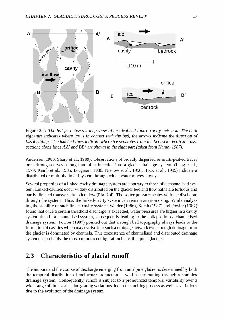
B’B
Figure 2.4: The left part shows a map view of an idealized linked-cavity-network. The darksignature indicates where ice is in contact with the bed, the arrows indicate the direction ofbasal sliding. The hatched lines indicate where ice separates from the bedrock. Vertical cross-sections along lines AA’ and BB’ are shown in the right part (taken from Kamb, 1987).
Anderson, 1980; Sharp et al., 1989). Observations of broadly dispersed or multi-peaked tracerbreakthrough-curves a long time after injection into a glacial drainage system, (Lang et al.,1979; Kamb et al., 1985; Brugman, 1986; Nienow et al., 1998; Hock et al., 1999) indicate adistributed or multiply linked system through which water moves slowly.
Several properties of a linked-cavity drainage system are contrary to those of a channelised sys-tem. Linked-cavities occur widely distributed on the glacier bed and flow paths are tortuous andpartly directed transversely to ice flow (Fig. 2.4). The water pressure scales with the dischargethrough the system. Thus, the linked-cavity system can remain anastomosing. While analyz-ing the stability of such linked cavity systems Walder (1986), Kamb (1987) and Fowler (1987)found that once a certain threshold discharge is exceeded, water pressures are higher in a cavitysystem than in a channelised system, subsequently leading to the collapse into a channeliseddrainage system. Fowler (1987) pointed out that a rough bed topography always leads to theformation of cavities which may evolve into such a drainage network even though drainage fromthe glacier is dominated by channels. This coexistence of channelised and distributed drainagesystems is probably the most common configuration beneath alpine glaciers.
2.3 Characteristics of glacial runoff
The amount and the course of discharge emerging from an alpine glacier is determined by boththe temporal distribution of meltwater production as well as the routing through a complexdrainage system. Consequently, runoff is subject to a pronounced temporal variability over awide range of time scales, integrating variations due to the melting process as well as variationsdue to the evolution of the drainage system.

CHAPTER 2. GLACIAL HYDROLOGY: A PROCESS REVIEW 18
2.3.1 Variability due to meltwater generation processes
Longterm variability
From a longterm perspective, a glacier represents a hydrological storage. Most of the annualprecipitation falls as snow, thus, it contributes to mass storage rather than directly to runoff(Röthlisberger and Lang, 1987). Hence, the glacier mass balance is equivalent to the storagechange component in the glacier’s water budget. During times of negative mass balance, wateris released from this storage and contributes to runoff. In contrast, a positive glacier massbalance is associated with a cool and wet ablation season, resulting in decreased total runoff.This inverse relationship of glacier runoff and precipitation is referred to as the “compensatingeffect” (Röthlisberger and Lang, 1987). Through this coupling to the glacier mass balance, theamount of glacial discharge is controlled by climatic variations.
Seasonal variability
The annual cycle of glacier runoff is primarily governed by the course of solar radiation andair temperature. The radiation dependence implies also a large influence by the retreat of thetransient snow-line. Subjected to identical meteorological conditions, more meltwater would beproduced late in the ablation period when large areas of dark ice are exposed to the surface ascompared to the beginning when those areas are covered by high albedo snow. Similarly, as aresult of this albedo-effect, a pronounced discharge decline is observed after summer snowfalls(Fig. 2.5) (Röthlisberger and Lang, 1987; Escher-Vetter and Reinwarth, 1994; Braun, 1996).
Diurnal variability
Due to the dominance of meltwater production by solar radiation and air temperature, meltingoccurs predominantly during the day whereas it is strongly reduced at night. This producesa diurnal hydrograph cycle which is characteristic for the runoff from glaciers. Figures 2.5and 2.6 demonstrate how this diurnal variation is superimposed to a base flow varying on aseasonal time scale and that high discharges coincide with large diurnal variations (Elliston,1973; Röthlisberger and Lang, 1987).
2.3.2 Variability due to routing processes
As shown above, water can be transferred through a glacier by different drainage systems. Assuch, the initial temporal distribution of meltwater supply is modified. The primary hydrologicaleffects of the firn and transient snow-cover is the retention of meltwater and its delay due to slowpercolation velocities (Oerter and Moser, 1982; Fountain and Walder, 1998; Schneider, 1999).Consequently, runoff concentration is accelerated as the snow line retreats during the summerseason or as the thickness and extend of the firn area is decreased during periods of negativemass balance (Braun, 1996).
Since the geometry of englacial and subglacial drainage configurations is controlled by the rateof discharge as well as by creep-closure of the ice, most passageways decrease considerably insize during winter, when no surface meltwater is produced (Röthlisberger and Lang, 1987). In

CHAPTER 2. GLACIAL HYDROLOGY: A PROCESS REVIEW 19
June July August September
1991
02
4
6
810
disc
harg
e [m
3 s−
1 ]
Figure 2.5: Hydrograph of hourly means of discharge from Vernagtferner as measured duringthe ablation season June to September 1991, (taken from Escher-Vetter and Reinwarth (1994)).
6: 8: 10: 12: 14: 16: 18: 20: 22: 0: 2: 4:time
0
2
4
6
disc
harg
e [m
3 s−
1 ]
1991MayJuneJulyAugSepOct
Figure 2.6: Mean diurnal variation of discharge from Vernagtferner during the ablation seasonJune to September 1991. The faster arrival of peak discharge as the season progresses is clearlynoticeable, (taken from Escher-Vetter and Reinwarth (1994)).

CHAPTER 2. GLACIAL HYDROLOGY: A PROCESS REVIEW 20
contrast, a cavity system is kept open mainly by basal sliding and only secondarily by melting.Therefore it is likely to persist throughout the winter (Fountain and Walder, 1998) by drainingsubglacially produced water (Lliboutry, 1983). At the beginning of the melt season the capacityof the basal drainage system is not sufficient to cope with the actual meltwater flux. Withincreasing discharge the linked cavity system becomes unstable (Walder, 1986; Kamb, 1987;Fowler, 1987) resulting in the formation of hydraulically efficient channels. In response toa progressively rising meltwater supply, the channelised system expands up-glacier over thecourse of the season (Nienow et al., 1998). The evolution of discharge routing through a glacieris determined by two processes. First, retention decreases due to a reduction in the thicknessand extent of the snow and firn cover and second, the en- and subglacial systems develop ahigher drainage capacity. Figure 2.6 displays this behavior in the faster arrival of the dailydischarge peak as the season progresses (Elliston, 1973; Escher-Vetter and Reinwarth, 1994;Braun, 1996).
Aperiodic variability
Additional runoff variability is induced by discharges of water derived from rainfall onto theglacier surface. Further, water can be stored temporarily in isolated en- or subglacial waterpockets and cavities or ice-dammed lakes. The sudden release of such water causes erraticvariations in runoff which are not directly triggered by climatic variations (e.g. Luetschg, 1926;Liestøl, 1956; Röthlisberger, 1981; Clarke, 1982; Haeberli, 1983; Bjørnsson, 1998; Andersonet al., 1999).

Chapter 3
Water balance
Balancing the water input with discharge output provides a possibility to investigate the evolu-tion of a glacial drainage system. An imbalance of input and output would indicate temporarystorage of water in or beneath the glacier. Subglacial storage of water can be related to theinability of the prevailing drainage system to discharge water at the same rate as it is suppliedto the system. This is especially likely to occur at the beginning of the ablation season whenlarge amounts of meltwater are rapidly transferred into an inefficient winter drainage system(Sec. 1.1.1).
During the 1999 summer field season we conducted an extensive field program at Unteraar-gletscher comprising glaciological, meteorological and hydrological measurements. In thischapter, we want to assess the storage of water in or beneath the glacier early in the melt sea-son, when a rearrangement of the subglacial drainage system and mechanical adjustments at theglacier bed are likely to occur. Meltwater input to the glacial hydrological system was quanti-fied using a temperature index melt model which was calibrated with ablation measurements.Discharge was measured at a gauging station in the proglacial stream. However, 18 days afterits installation, the station was destroyed during a flood event which was presumably caused bya rainfall-induced outburst of en- or subglacially stored water. We discuss this outburst flood inlight of a significant imbalance of water input and output during the days preceeding the releaseevent and a change in the configuration of the drainage system.
3.1 Methods
3.1.1 Meteorological records
At the Lauteraarhut (Fig. 1.1) we operated an automatic weather station to collect data on airtemperature, relative humidity, wind speed, wind direction and precipitation at intervals of 15minutes. Only the air-temperature and precipitation measurements (Fig. 3.1) are of relevanceto the work presented here. Air temperature was measured by a ventilated thermistor (VaisalaT107) and precipitation was measured using a tipping bucket rain gauge (Joss-Tognini). Wechose a measurement site beside the glacier rather than directly on the glacier because thermalconditions of the near surface boundary layer adjacent to the glacier are less affected by localprocesses such as catabatic winds, condensation and evaporation than those on the glacier itself(Lang and Braun, 1990).
21

CHAPTER 3. WATER BALANCE 22
Jun. Jul. Aug. Sep.1999
−5
0
5
10
15
20
tem
pera
ture
[o C]
403020100
prec
. [m
m d−
1 ]
a
b
Figure 3.1: Daily values of (a) total precipitation and (b) mean air temperature as recorded atthe Lauteraarhut during the ablation season 1999.
3.1.2 Determination of surface melt
Water originating from surface melt was the main input into the hydrological system of Un-teraargletscher during the period in which the interest of this study is focused on. To quantifythis meltwater input, point measurements of ablation were used to calibrate a distributed meltmodel (Sterr, 2000; Hock, 1999). Liquid precipitation may also contribute to the water input buta quantification of the precipitation over the entire catchment is not performed in this study. Thecomplex spatial distribution of precipitation in a mountainous catchment would require a studyon its own. Thus, in the remainder of this thesis the contribution of precipitation is neglectedsuch that the term “input” as used here represents a minimum estimate.
Ablation measurements
Melt was monitored between June and September 1999 at up to 26 ablation stakes distributedacross the ablation area of Unteraargletscher (Fig. 3.2) by taking stake readings on four occa-sions at intervals of 2–5 weeks. However, only at 14 stakes the measurements were performedfour times. Nevertheless, for some intervals between individual stake readings the dataset iscomplete. In addition, the thickness of the snow cover at the beginning of the observation periodwas measured at four locations at different altitudes. To convert these thickness-measurementsinto water-equivalent (w.e.) melt, we use a typical density of 500 kg m−3 for wet snow and adensity of 900 kg m−3 for ice (Paterson, 1994).
Melt model
Snow and ice melt across the entire glacier was estimated using a distributed temperature-indexmethod developed by Hock (1999) that includes direct clear-sky solar radiation. The method is
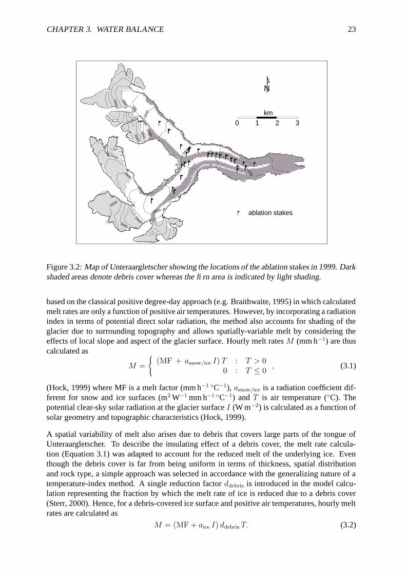
CHAPTER 3. WATER BALANCE 23
3000
2800
2600
3000
2200
0 1 2 3
km
N
0003
2600
0082
2400
ablation stakes28003000
3200
2600
2800
Figure 3.2: Map of Unteraargletscher showing the locations of the ablation stakes in 1999. Darkshaded areas denote debris cover whereas the firn area is indicated by light shading.
based on the classical positive degree-day approach (e.g. Braithwaite, 1995) in which calculatedmelt rates are only a function of positive air temperatures. However, by incorporating a radiationindex in terms of potential direct solar radiation, the method also accounts for shading of theglacier due to surrounding topography and allows spatially-variable melt by considering theeffects of local slope and aspect of the glacier surface. Hourly melt rates M (mm h−1) are thuscalculated as
M =
{
(MF + asnow/ice I) T : T > 00 : T ≤ 0
, (3.1)
(Hock, 1999) where MF is a melt factor (mm h−1 ◦C−1), asnow/ice is a radiation coefficient dif-ferent for snow and ice surfaces (m2 W−1 mm h−1 ◦C−1) and T is air temperature (◦C). Thepotential clear-sky solar radiation at the glacier surface I (W m−2) is calculated as a function ofsolar geometry and topographic characteristics (Hock, 1999).
A spatial variability of melt also arises due to debris that covers large parts of the tongue ofUnteraargletscher. To describe the insulating effect of a debris cover, the melt rate calcula-tion (Equation 3.1) was adapted to account for the reduced melt of the underlying ice. Eventhough the debris cover is far from being uniform in terms of thickness, spatial distributionand rock type, a simple approach was selected in accordance with the generalizing nature of atemperature-index method. A single reduction factor ddebris is introduced in the model calcu-lation representing the fraction by which the melt rate of ice is reduced due to a debris cover(Sterr, 2000). Hence, for a debris-covered ice surface and positive air temperatures, hourly meltrates are calculated as
M = (MF + aice I) ddebris T. (3.2)

CHAPTER 3. WATER BALANCE 24
Table 3.1: Model parameters optimized for Unteraargletscher
Parameter Value UnitAir temperature lapse rate −0.65 ◦C (100 m)−1
Melt factor 1.875 × 10⁻² mm h−1 ◦C−1
Radiation factor for ice 0.7 × 10⁻³ m2 W−1 mm h−1 ◦C−1
Radiation factor for snow 0.5 × 10⁻³ m2 W−1 mm h−1 ◦C−1
Reduction factor for debris 0.65 -
Rates of snow and ice melt were computed using Equations 3.1 and 3.2 for each gridcell of a50 m resolution digital elevation model (DEM) of Unteraargletscher that was constructed from1998 aerial photographs. To account for the shading of the glacier surface due to surroundingtopography, the glacier DEM was embedded within the Swiss 1:25000 digital elevation modelDHM25 of the entire surrounding catchment area (L+T, 1993). Slope and aspect angles ofeach gridcell were directly derived from the DEM. In addition, topographic shading of theglacier was determined for every time step and each gridcell based on the effective horizonand the position of the sun. The melt model further requires a digital model of the glaciersurface type beneath the winter snow cover (Hock, 1999). This surface type was prescribed byraster maps, indicating for each gridcell whether the surface was ice, firn or debris (Fig. 3.2).For the purpose of melt rate calculation the model treats firn like snow. Spatial distributionof debris and firn were derived from aerial photographs. A further raster map contains thedistribution of the initial snow cover on the glacier which is based on a linear interpolationof snow thickness measurements, ranging from 0.15 m w.e. at 2200 m a.s.l. to 0.5 m w.e. at2400 m a.s.l. and 1.0 m w.e. at 2550 m a.s.l..
Required input data for the model is air temperature. The temperature recorded at the auto-matic weather station (Fig. 3.1) was extrapolated and distributed to each gridcell using a linearlapse rate. The melt factor, radiation coefficients for snow and ice, and debris reduction factorare empirical coefficients. Together with the temperature lapse rate, these coefficients are thecalibration parameters of the model.
The melt simulations were initialized using model parameters which have been optimized forStorglaciären, Sweden, by Hock (1999). Subsequently, these parameters were adjusted itera-tively to achieve maximum agreement between computed and measured melt rates at the abla-tion stakes (Sterr, 2000). Typically model runs were performed for the period that begins withthe start of the temperature record on 19 June and ends on 8 September 1999 when the finalablation stake readings were taken. Parameter optimization involved the visual inspection ofplots of simulated and measured melt for three different periods that coincided with the inter-vals between the ablation stake measurements. Table 3.1 lists the model parameters optimizedfor Unteraargletscher.
Model performance
The spatial distribution of the calculated melt (Fig. 3.3) compares favorably with what we ex-pect when we bear in mind the effects of topography on shading and potential direct solarradiation. Values of calculated radiation averaged over the entire observation period 19 June to

CHAPTER 3. WATER BALANCE 25
1000
2000
3000
4000
5000melt [mm w.e.]
N
Figure 3.3: Spatial distribution of the calculated melt (mm w.e.) on Unteraargletscher, cumu-lated over the entire observation period 19 June – 8 September 1999.
8 September range between a minimum of 17 and a maximum of 314 W m2. Melt on south-facing slopes typically exceeds that on north-facing slopes. In addition, the effect of the debriscover is also clearly visible. The highest melt is calculated for debris-free zones at the northernside of the tongue of the glacier and between the medial moraines. In contrast, calculated meltis drastically reduced in the debris-covered terminus region.
Fig. 3.4 shows simulated and measured melt at 14 ablation stakes distributed across the ablationarea of the glacier for the entire observation period (19 June – 8 September). Melt simulationand measurement as a function of time at two stakes are compared in Fig. 3.5. Consideringthe simplicity of the model, there is good agreement between ablation measurements and meltsimulation (Fig. 3.4b). While at some stakes the model overestimates melt, at others ablation isunderestimated (Fig. 3.4a). Nevertheless we want to note that a direct comparison of measuredmelt with that calculated by the model is not without problems because simulations representthe spatial means of 50 m by 50 m gridcells, whereas stake measurements refer to an individualpoint inside each of these areas.
A notable feature in Fig. 3.4a is that melt at higher altitudes is significantly larger than thatin the lower reaches of the glacier. The lower melt at lower altitudes reflects reduced ablationdue to debris covering much of the tongue of Unteraargletscher as most of the stakes belowthe confluence zone (2400 m a.s.l.) are located in debris-covered ice (triangles in Fig. 3.4a).The insulating effect of the debris cover is also revealed in plots of melt versus time (Fig. 3.5).Melt at a stake located in debris-covered ice on the medial moraine ((a) in Fig. 3.5) is roughlyhalf as large as that at a stake located ∼150 m higher in altitude but in debris-free ice ((b) inFig. 3.5). However, prior to the retreat of the snowline past these two stakes at the end of June,the snowcover at these locations is melted roughly at the same rate.
The performance of the melt model can be further assessed by comparing the simulated retreat

CHAPTER 3. WATER BALANCE 26
2150 2200 2250 2300 2350 2400 2450 2500elevation [m a.s.l.]
01000
2000
3000
40005000
mel
t [m
m w
.e.]
0 2000 4000measured melt [mm w.e.]
0
2000
4000
calc
ulat
ed m
elt [
mm
w.e
.]
r2 = 0.92
a b
Figure 3.4: (a) Measured (filled symbols) and simulated (open symbols) melt (mm w.e.) at 14ablation stakes for the entire observation period 19 June – 8 September 1999. Diamonds andtriangles denote stakes that are located in debris-free and debris-covered ice, respectively. (b)Measured vs simulated melt.
Jun. Jul. Aug. Sep.
1999
0
1000
2000
3000
4000
5000
cum
ulat
ive
mel
t [m
m w
.e.]
a
b
Figure 3.5: Simulated (solid line) and measured (diamonds) melt (mm w.e.) vs time at (a) astake located in debris-covered ice on the medial moraine (2217 m a.s.l.) and (b) a stake locatedin debris-free ice (2376 m a.s.l.).

CHAPTER 3. WATER BALANCE 27
0
2000
a b
snow depth(mm w.e.)
Figure 3.6: Spatial distribution of the snow cover on Unteraargletscher. (a) Simulated snowdepth (mm w.e.) on 24 July 1999. (b) Photograph showing the snowline (dashed line) on 26July 1999 (photograph taken by T. Schuler).
of the snow line with that observed on the glacier. The close agreement of the location of thesnow line as identified on a photograph taken on 26 July (dashed line in Fig. 3.6b) and that asdetermined from the calculated snow depth distribution on 24 July 1999 (Fig. 3.6a) suggeststhat the spatial pattern of snow melt is reproduced reasonably well by the model calculations.
3.1.3 Glacial runoff
Stage recording
Most of the glacial runoff exits Unteraargletscher through a single large glacier portal. However,because the proglacial area consists of a flat alluvium, the stream is strongly braided before itreaches Lake Grimsel and single branches change their position frequently by lateral and ver-tical erosion. Only at a few locations flow is concentrated in a single thread. About 500 mdownstream of the glacier terminus, the stream is incised into a former terminal moraine offer-ing a moderately stable cross-section. All hydrological measurements were performed at thislocation which is referred to as the gauging site (Fig. 1.1 and 3.7).
Water stage was measured using a vented capacitive pressure transducer (Keller PR-46W) andelectrical conductivity was measured with a commercial conductivity probe (Campbell 247).Conductivity readings were corrected for errors resulting from ionisation and temperature ef-fects according to technical instructions by the producer (Campbell, 1994). Both sensors werehoused inside a gauging device that consists of two 1.2 m long concentric PVC cylinders havingdiameters of 20 and 30 cm. The device was positioned vertically in the stream and fastened tosteel pipes that were anchored at the stream bank by a 4.5 m3 sized gabion filled with boulders(Fig. 3.8). The inner cylinder is closed at its lower end. A set of four 10 mm diameter holesclose to the bottom allows water to pass through the cylinder while at the same time effectivelydamping high frequency water level fluctuations. The outer cylinder serves as a protection frommechanical damage and reduces the accumulation of sediment within the inner cylinder. Outputfrom both sensors were recorded by a Campbell CR-10 data logger every 5 minutes.

CHAPTER 3. WATER BALANCE 28
salt injections
~ 500 m
glacierterminus
moraine
N
not to scale
moraine
gauging site: stage & conductivity (1999, 2000), fluorometry (2000)
Figure 3.7: Schematic sketch showing the approximate locations of installations in theproglacial area. Streamflow is towards east.
Discharge measurements
To relate water stage to glacier runoff 22 individual discharge measurements were performedin the proglacial stream using the tracer-dilution method which is particularly suited to mea-surements at conditions of highly turbulent flows and unstable stream configurations (Fischer,1982; Käss, 1998). The method entails the injection of a tracer in the stream and its subsequentdetection at an appropriate distance downstream assuming that the tracer is uniformly mixedover the entire cross-section of the stream at the detection point. Additional assumptions arethat discharge does not change significantly during the course of a measurement and that thereare no sources and sinks of water between the points of tracer injection and detection. For theproglacial stream of Unteraargletscher the minimum flow distance necessary to ensure uniformmixing of the tracer with the stream water was estimated between 200 and 500 m (Käss, 1998).
We injected amounts of 5 to 10 kg of solid sodium chloride (NaCl) ∼500 m upstream from thegauging station (Fig. 3.7). We found that the results were unaffected by not dissolving the salt instream water prior to injection. Following a salt injection, electrical conductivity was recordedat intervals of one second until the entire salt wave had passed the gauging station and conduc-tivity values had essentially returned to the background level. The salt concentration c (kg m−3)in the stream water is derived from the measured electrical conductivity L (µS mm−1) by apply-ing the linear relationship c = kL, where the constant k = 7.36×10⁻³ (kg m−3)/(µS mm−1) wasdetermined by calibrating the instrument with solutions of known salt concentration. DischargeQ (m3 s−1) is then calculated using the mass-balance relationship
Q =m
τ∫
0(c(t) − c0) dt
, (3.3)
where m (kg) is the mass of salt injected, τ is the time it takes for the entire salt wave to pass the

CHAPTER 3. WATER BALANCE 29
Figure 3.8: The gauging station in June 1999. The terminus of Unteraargletscher can be seen inthe background (photograph taken by T. Schuler).
gauging station, and c0 = kL0 is the background concentration. The background conductivityL0 was determined as a linear interpolation of 10 second averages before and after the passageof the salt wave (Fig. 3.9).
Discharge measurements were carried out repeatedly throughout the entire period of stage mea-surements that extended from 16 June when the stream gauge was installed to 4 July when thedata was downloaded for the last time before the gauging station was destroyed. Furthermore,the measured discharges cover the whole range of observed water stages. The stage–dischargerelation is obtained using the water stage measurements hs (m) at the time of the dischargemeasurement. The resulting rating curve
Q = e 3.82 hs + 1.564 (3.4)
is constructed as the best fit to the data points (Fig. 3.10). The exponential form of the ratingcurve reflects the increasing width of the stream as the water level rises.
3.2 Results
3.2.1 Input into glacial system
The modeled melt rate (Fig. 3.11c) displays pronounced diurnal variations which primarily re-flect the distinct daily cyclicity of the direct clear-sky solar radiation. While the calculated meltrates are nearly zero during night time, they peak sharply at mid day when the potential solarradiation reaches its daily maximum. In addition, the daily melt rate maxima are modulated bythe general course of the temperature record (Fig. 3.11b). Warm temperatures in early July re-sult in a high meltwater production. The highest melt rate of the entire period of melt simulation(19 June - 8 September), exceeding 40 m3 s−1 integrated over the glacier area, is calculated for

CHAPTER 3. WATER BALANCE 30
:0 :2 :4 :6 :8 :10 :12 :14 :16 :18 :20 :22 :24 :26 :2820:
time [hh:mm]
0.008
0.010
0.012
0.014co
nduc
tivity
[mS
cm−
1 ]
Figure 3.9: Example of an individual discharge measurement using the salt dilution method.The vertical lines indicate the duration of the tracer passage. The dotted area represents theconcentration integral in the denominator of Equation 3.3.
3 July. Conversely, meltwater production ceases completely during periods with temperatureswell below 0◦C on 21 and 22 June.
To quantify the uncertainty of the melt calculation we determined the standard deviation ofsimulated melt with respect to measured melt. For the 14 stakes that are available for theentire period, calculated melt deviates from measurements by ±390 mm w.e.. Taking a meanmeasured ablation of 2290 mm w.e., this deviation translates into a ±17% uncertainty in ourmelt simulations. The number of stakes available for the shorter intervals between individualablation measurements is larger but uncertainties are similar varying between ±13% and ±16%.An exception is the two week interval between the first two stake readings where the uncertaintyamounts to ±44%. However, the calculation of this high uncertainty is likely affected by twoartifacts. First, measurement and simulation do not refer to the same length of time. Thefirst stake readings were taken on 16 June, three days before the starting date of the modelcalculation. In effect, we are comparing measured and calculated melt over time intervals thatdiffer in length by ∼20%. Second, during these two weeks at the end of June, the medialmoraine became partly snow-free, resulting in a pronounced micro-scale variability of melt dueto the discontinuous snow coverage which is not accounted for in the conceptual melt model.Therefore, we disregard the ±44% uncertainty determined for this two week interval and accepta generous overall uncertainty of ±20% for our melt calculations.
3.2.2 Output from glacial system
The recorded discharge (Fig. 3.11d) varies between 2.8 and 7.6 m3 s−1 and shows a diurnal cyclethat is characteristic for glacial runoff (Röthlisberger and Lang, 1987). Typically, dischargemaxima occur in the early evening followed by discharge minima in the morning of the next

CHAPTER 3. WATER BALANCE 31
0.0 0.1 0.2 0.3 0.4 0.5stage [m]
2
4
6
8
disc
harg
e [m
3 s−
1 ]
Figure 3.10: Discharge rating curve for the proglacial stream of Unteraargletscher. Error barsare ±10%. The solid line represents Equation 3.4 over the entire range of measured waterstages.
day. Superimposed on these diurnal variations are secondary spikes that can be associatedwith precipitation events on 21, 26, 27 and 28 June (Fig. 3.11a). In general, we note a period ofrecession flow lasting from 19 to 25 June followed by an increase in discharge during the secondpart of the record. Coinciding with increasing discharge the amplitude of the diurnal cycle isalso enlarged. Furthermore, towards the end of the period of observation discharge varies lesssmoothly and the record displays a jagged appearance. These small but rapid fluctuations areattributed to enhanced bed load transport at high discharges.
We believe that the main source of error in our rating curve and discharge measurements stemsfrom the unstable stream configuration due to an unconsolidated nature of the stream bed. Inparticular, erosion and sedimentation processes within the stream can lead to changes in waterlevel that are unrelated to variations in discharge. A number of discharge measurements atlow water stages (cluster of data points in the lower lefthand corner of Fig. 3.10) suggests thatdischarge measurements can vary by roughly ±0.2 m3 s−1 for nearly the same water level. For adischarge of ∼3 m3 s−1, this variability corresponds to less than the ±10% accuracy which hasbeen reported for comparable situations (Anderson et al., 1999; Kite, 1994). In contrast, noise inthe stage measurements that results from the roughness of the water surface inside the gaugingdevice is considered to be small except maybe at very high discharges. Other sources of errorare associated with the calibration of the pressure transducer and the salt-dilution measurementsof discharge themselves. As an overall estimate, we assign an uncertainty of ±10% to ourdischarge measurements.
3.2.3 Water balance
In general, the diurnal variations of glacial runoff from Unteraargletscher reflect those of melt-water input to the glacier. Daily maxima and minima of discharge (Fig. 3.11d) lag behind those

CHAPTER 3. WATER BALANCE 32
17 18 19 20 21 22 23 24 25 26 27 28 29 30 1 2 3 4 5 6 7June July1999
2
4
6
8
0
15
30
45
−505
101520
128
40
precipitation [mm h−1]
temperature [oC]
melt rate [m3 s−1]
discharge [m3 s−1]d
c
b
a
Figure 3.11: Hourly values of (a) precipitation and (b) air temperature at the Lauteraarhut, (c)modeled melt rate of the entire glacier and (d) discharge in the proglacial stream.

CHAPTER 3. WATER BALANCE 33
of melt rate (Fig. 3.11c) and air temperature (Fig. 3.11b) by ∼3–5 hours which suggests thatrunoff was fed mainly by meltwater. However, for longer-term variations, temporal patterns ofsurface melt rate and glacial runoff show significant differences. With the arrival of a cold fronton 21 June, air temperature dropped drastically to values well below 0◦C causing the meltwaterproduction to fall to zero. In response to this reduced meltwater input to the glacier, dischargeof water in the proglacial stream started to decline. The return of higher temperatures on 23June led to an increase in meltwater production. However, discharge remained low for threefurther days. Subsequently, melt rates remained high and discharge increased until the end ofthe record.
17 18 19 20 21 22 23 24 25 26 27 28 29 30 1 2 3 4 5 6 7June July1999
0
5
10
15
cum
ulat
ive
mel
t or
disc
harg
e [
106 m
3 ]
melt
discharge
Figure 3.12: Cumulative melt of the entire glacier (solid line) and cumulative discharge in theproglacial stream (dashed line). The shaded regions show the uncertainties associated withdetermining melt and discharge (see text for details).
We illustrate the water balance further in Fig. 3.12 by plotting the cumulative meltwater inputand the cumulative discharge. The uncertainties in determining melt or discharge (shaded re-gions in Fig. 3.12) increase with time due to the cumulative nature of the plot. They are basedon the ±10% and ±20% uncertainties in our discharge measurements and melt calculations,respectively. During the first two days of the period shown in Fig. 3.12 meltwater input anddischarge output of water were roughly balanced. Due to low temperatures on 21 and 22 Junemeltwater production essentially ceased. However, discharge in the proglacial stream contin-ued, suggesting that water stored within the glacier was drained during these two cold days. Thetemperature rise on 23 June marks the start of a recharging period that lasted at least until theend of the discharge record on July 4. Most of this period is characterized by inputs in excess ofoutputs as more water was produced by melting on the glacier surface than was discharged inthe proglacial stream. After taking the uncertainties in determining melt and discharge (shadedregions in Fig. 3.12) into consideration, the surplus of water at the end of the discharge recordon 4 July amounts to ∼106 m3 (Fig. 3.12).

CHAPTER 3. WATER BALANCE 34
3.2.4 Rainfall-induced outburst
Following six days of warm conditions, a storm system brought torrential rainfall to Unteraar-gletscher in the early morning of 6 July (Fig. 3.11a and b). Nearly 40 mm of rain was recordedat the Lauteraarhut between 0000 and 1200 hours. In fact, this storm produced the highest con-tinuous rainfall amount during the entire period of observation from 19 June to 8 September(Fig. 3.1a). Coinciding with the intense rain, the discharge of water in the proglacial stream hadincreased dramatically. As a consequence, our stream gauge was completely destroyed. We es-timate that the discharge at mid day of 6 July was between 20 and 30 m3 s−1 which correspondsto roughly three times the maximum discharge recorded during the preceeding days. Due to thehigh discharge the stream bank at our gauging site had been eroded and the stream had changedits course. Furthermore, large chunks of ice (up to 0.8 m diameter) floated in the stream andwere strewn across much of the proglacial area.
3.3 Discussion
In this chapter, we have compared meltwater input and discharge output of water at Unteraar-gletscher during a two week period prior to a hydraulic release event. This comparison suggeststhat roughly 106 m3 more water was produced by melting of snow and ice on the glacier thanwas discharged in the proglacial stream implying that this water was stored in the glacial hy-drological system. The water storage may have been in any part of the glacier: within the snowand firn on the glacier surface, within englacial conduits and water pockets, or in cavities anddrainage channnels at the bed.
To assess the extent to which water was stored in or beneath the glacier, we have to investigatethe capacity of the snowpack covering the glacier to retain water. At the beginning of ourmeasurement program in mid June, we noticed small streamlets and slush areas on the snowsurface up to an elevation of at least 2600 m a.s.l. The occurrence of water at the surface issymptomatic for a snow cover which is water saturated. Thus, no further retention of waterwas possible and any meltwater produced in the region of the glacier below 2600 m a.s.l. musthave contributed to either runoff or en- and subglacial storage. For the region of the glacierabove 2600 m a.s.l. we do not know the degree of water saturation of the snow cover, renderingit difficult to determine whether meltwater that percolated into the snow was retained or wasdelivered to the glacier. To simplify our discussion we now focus on the region of the glacierbelow 2600 m a.s.l. Computation of melt for this region yields a total amount of ∼6.5× 10⁶ m3
of water for the period from 19 June to 4 July. This amount alone is sufficient to balance thetotal discharge of water from the glacier during the same period (∼5.9 × 10⁶ m3). We note,however, that our melt calculation led to a conservative estimate of the water input to the glacialhydrological system because snow melt from the non-glacierized portion of the catchment isnot accounted for. Furthermore, the rise in snowline from the terminus to the confluence zoneduring this period released meltwater that was detained in the snowpack earlier in the season.Therefore, this additional meltwater originating from both the surrounding non-glacierized areaand the disappearing snow cover together with the contribution from precipitation in liquidform (∼43 mm at the Lauteraarhut between 19 June and 4 July), when factored into the waterbalance, lead to inputs of water in excess of discharge outputs that had to be stored within or atthe base of Unteraargletscher.

CHAPTER 3. WATER BALANCE 35
2 3 4 5 6 7 8 9 10July1999
100
150
200
250
300
wat
er le
vel [
m]
Figure 3.13: Variations of water level in a 250 m deep borehole drilled to the bed of Unteraar-gletscher. The dashed line denotes the water level that corresponds to flotation pressure.
The flood in the proglacial stream that coincided with a severe rain storm early on 6 July presum-ably reflects the outburst of the water that was stored en- or subglacially during the preceedingdays. The large ice chunks that were spewed out and strewn across much of the proglacialarea during this event suggest that the peak discharge of water early in the morning was con-siderably larger than the 20 – 30 m3 s−1 we estimate for mid day of 6 July. However, thesechunks were probably not derived subglacially as they can be attributed to a collapse of iceat the glacier portal. Nevertheless, we believe that the outburst flood is related to a change inthe configuration of the subglacial drainage system. Support for this suggestion stems from arecord of water level fluctuations (Fig. 3.13) in a 250 m deep borehole drilled through the iceto the bed near the central flowline, roughly 3 km upglacier from the terminus (Fig. 1.1). Di-urnal variations in borehole water level were in phase with those of discharge in the proglacialstream during the days preceeding the release event which suggests that the hole was hydrauli-cally connected to the drainage system. With the onset of precipitation in the afternoon of 5July (Fig. 3.11a), the water level quickly rose indicating a sudden increase in subglacial wa-ter pressure to near flotation level (Fig. 3.13). Subsequently, the water level fluctuated wildlybefore the borehole lost its connection to the drainage system and filled with water. The fastrise in water pressure is thought to reflect the inability of the drainage network to adapt to thesudden increase in water supply caused by the rain. We conjecture that in response to highbasal water pressure, water was forced to spread out at the ice–bed interface thereby alteringconfigurations, dimensions and positions of exisiting drainage pathways. During the course ofthis basal drainage-system reorganization, the borehole became hydraulically isolated, whilethe establishment of a hydraulically efficient drainage net elsewhere enabled the fast release ofen- and subglacially stored water.
In summary, a warm weather period at Unteraargletscher in late June and early July producedmeltwater at a rate greater than the glacial drainage system could transmit. Consequently, waterstorage in and beneath the glacier increased. This warm period culminated in a storm withintense rain which caused water flow to back up further and subglacial water pressure to rise.
CHAPTER 3. WATER BALANCE 36
The high water pressure triggered a reorganization of the basal drainage system which in turnled to the release of water that was stored in and beneath the glacier.

Chapter 4
Tracer tests and their analysis
4.1 Principles of tracer experiments
Tracing techniques are widely used in hydrology to investigate manifold issues including deter-mination of ground water trajectories, residence times and also quantitative characterization ofdrainage systems and measuring discharge rates (see also Sec. 3.1.3). In principle, the techniqueconsists of labelling water at its entry into an unknown system and the subsequent detection ofthe marker after its passage through that system. An extensive compilation of the developmentin tracing techniques from first simple applications to modern experiments is found in Käss(1998). Today tracer techniques are important tools for research on virtually inaccessible hy-drological systems and processes. In contrast to measurements at an individual point, thesemethods impart direct information on the flow characteristics integrated from an input locationto a site of detection. Therefore, tracer tests have been used quite early as a preferred methodfor investigating glacial drainage systems. Tracer experiments made a significant contributionto the understanding of glacial hydrology (Röthlisberger and Lang, 1987). Tracing the waterthat percolates through the firn or flows into moulins or at the bottom of boreholes had sub-stantial implications for the identification of distinct drainage types, delimiting catchments andinferring hydraulic conditions (Fountain and Walder, 1998; Hubbard and Nienow, 1997).
4.1.1 Requirements on tracers
Tracer experiments provide information about hydraulic conditions of a drainage system if thetracer transport is identical to the flow of individual water particles. Today’s tracing techniquescome close to this ideal. Furthermore, the ’ideal tracer’ requires the satisfaction of a number ofconditions. The substance should possess optimal dissolubility in water, physical and chemicalstability and high resistance against adsorption to the surrounding substratum or the suspendedsediments. Besides these primary qualities, tracer should be detectable at low concentration in-dependent of temperature and pH. And further, the natural background concentration should beas low as possible. Additionally, questions as to whether the substance is ecologically harmless,available in the necessary quantity and cost-effective play a role in the choice of an appropriatetracer.
37

CHAPTER 4. TRACER TESTS AND THEIR ANALYSIS 38
4.1.2 Properties of fluorescent dyes and other tracers
For glacio-hydrological purposes, primarily fluorescent dyes are used as tracers since they meetthe mentioned requirements closest. Nevertheless, the use of salt and other substances has alsobeen reported (Stenborg, 1969; Kohler, 1995; Grust et al., 2001).
The use of fluorescent dyes in glacio-hydrological research traces back to the beginning of the20th century (Forel, 1898; Mercanton, 1916). Initially, the method exploited the extreme col-oring properties of such dyes, permitting visible detection (Käss, 1998). Today, this qualitybecomes irrelevant since modern detection methods are based on fluorometry. A fluorescentmolecule has the ability to absorb light at one wavelength and almost instantaneously emitlight at a different and longer wavelength. Fluorescence typically occurs about 10−8 s after themolecule absorbed the exciting light. The wave bands at which light is absorbed or emitted arespecific for the fluorescent. Fluorescence intensity is directly proportional to the concentrationof fluorescent solutes (Turner, 1997), thereby providing an efficient technology to detect dyetracers. Exploiting the knowledge about excitation and emission wavelength for a specific fluo-rescent, it became possible to detect dye down to concentrations of 0.01 ppb (parts per billion).The sensitivity of the fluorometric analysis depends on the efficiency of the dye in convert-ing excitation energy into fluorescence (Smart and Laidlaw, 1977). This property depends onthe temperature and water quality of the sample which can affect a dye’s fluorescence yield.In general, fluorescence intensity varies inversely with temperature, though this dependence isspecific for each dye. Some dye’s fluorescence is suppressed considerably at low pH values. Intypical glacial runoff reducing effects on fluorescence due to salinity or presence of fluorescentorganic matter can be excluded whereas other factors can be significant. In particular, highsuspended sediment concentrations coinciding with high turbidity values are likely to occur inrunoff from glaciers and can produce misleading background concentrations. Adsorption oftracer on substratum or suspended sediment surfaces is mainly irreversible and can thereforecause significant dye losses. Some fluorescent dyes are subject to photochemical decay limitingtheir usage in surface water (Smart and Laidlaw, 1977; Käss, 1998).
NaCl-salt can also be used as a suitable tracer, when fast flowing currents of low conductivewater should be labeled (Sec. 3.1.3). The natural background in glacial meltwater is typicallylow, thus providing a clear tracer signature while the detection is simply achieved via the elec-trical conductivity at low costs. On the other hand, the low detection sensitivity requires theinjection of large quantities, often representing a logistical limitation for an application at re-mote locations. The use of such tracers is therefore restricted to experiments where low outputconcentrations are not expected or not of interest.
Knowledge of both, dye tracer properties as well as some physical and chemical characteristicsof the investigated flow system is necessary to select the dye appropriate to the experiment. Thistask sometimes requires pilot investigations.
4.2 Transport models
To interpret the observed tracer-return curves we are faced with a typical inverse problem. Theway in which the tracer reappears after passage through an unknown system is determined bythe geometry of and the hydraulic conditions prevailing in that system. Visual inspection of theobserved return curve can already provide some general information on the configuration of the
CHAPTER 4. TRACER TESTS AND THEIR ANALYSIS 39
drainage system (Hock and Hooke, 1993; Nienow, 1993). The application of more objectivemethods is required to obtain further insight into system properties. Intrinsically, a tracer re-turn curve represents the residence time distribution of a specific system under given hydraulicconditions (Jury and Roth, 1990). A quantitative evaluation of curve characteristics allows theinference of system properties such as flow velocity and the degree of tracer spreading duringtransit. Reliable estimates for those quantities can be obtained by carefully fitting parameters ofa transport model to the observed data. However, an appropriate choice of the transport modelis crucial for a reliable parameter estimate since only correct simulations and predictions oftracer data lead to a legitimate description of system properties (Beven, 2001). In particular,the adopted forward model should be capable of successfully predicting main characteristicsof the tracer return curve such as the onset of tracer breakthrough, the time and magnitude ofmaximum concentration and the duration of concentration recession.
Considering that a tracer return curve represents the response of an unknown and possibly com-plex system, the use of simple, conceptual models is imperative to avoid under-determination ofthe problem and therefore equifinality of different solutions and subsequent over-interpretationof the data (Beven, 2001). Furthermore, the following models are strictly valid only for a con-servative tracer, a legitimate assumption considering the careful selection of the tracer.
The following transport models, their specific solutions and the parameter optimization proce-dure are implemented in the software CXTFIT2.1 which was used for estimating the transportparameters. This code is provided by the U. S. Salinity Laboratory and uses a nonlinear least-squares optimization method (Marquardt, 1963) to derive parameters (Toride et al., 1999).
4.2.1 Advection-dispersion model
In the following, we assume that the tracer concentration c is distributed over the entire cross-section of the flow and the width of the system is very small compared to its longitudinal extent.Thence, the tracer transport is regarded as a one-dimensional problem along the flow directionx.
Mainly, the tracer is advected with a transit velocity v which corresponds to the mean flowvelocity along the flowpath
∂c
∂t= −v
∂c
∂x. (4.1)
Assuming a constant and homogeneous velocity field within a labeled water volume, the tracershould reappear at the detection site in a concentration distribution identical to its initial distri-bution. However, two main processes determine the dispersion of the tracer cloud: moleculardiffusion and dispersion. Molecular diffusion is the thermic motion of dissolved components(Brownian motion) and dispersion is due to differential local velocities as well as differentiallengths of flow trajectories (see Figure 4.1). Regardless of their different nature, both processesare usually described by a diffusion equation using a single hydrodynamic dispersion coefficientD (Taylor, 1954)
∂c
∂t= D
∂2c
∂x2. (4.2)
Furthermore, “dispersion” is used synonymously to “hydrodynamic dispersion coefficient”.The combined advection-dispersion equation for one-dimensional transport of a conservativetracer is written as
∂c
∂t= D
∂2c
∂x2− v
∂c
∂x. (4.3)

CHAPTER 4. TRACER TESTS AND THEIR ANALYSIS 40
fric
tion
indu
ced
diffe
rent
ial v
eloc
ities
diffe
rent
ial p
athl
engt
h of
traj
ecto
ries
Figure 4.1: Mechanisms of hydrodynamic dispersion.
With the initial condition of an instantaneous tracer injection
c(x = 0, t) =m
Qδ(t), (4.4)
where δ(t) is a Dirac delta function and m is the total mass of tracer injected into the water fluxQ, the problem can be solved analytically (Kreft and Zuber, 1978; van Genuchten and Wagenet,1989; Kinzelbach, 1992). At a distance x1, the concentration as a function of time is given by
c(t) =m
Q
x1
(4πDt3)1
2
exp(−(x1 − vt)2
4Dt). (4.5)
The two transport parameters v and D are obtained by a fitting procedure. Since D characterizesthe velocity inhomogeneities in the system, the c(t)-solutions of a transport functions are alsoreferred to as the travel time probability function (Jury and Roth, 1990).
4.2.2 Mobile-immobile model
Homogeneous flow conditions as assumed for the advection-dispersion model are rarely foundin natural systems. Tracer transport through a glacial drainage system is often affected bystorage-retardation processes which lead to a pronounced asymmetry of the return curves char-acterized by a slowly declining tail (e.g. Brugman, 1986; Seaberg et al., 1988; Willis, 1990;Fountain, 1993; Hock and Hooke, 1993; Nienow 1993). Behavior like this cannot be explainedby the advection-dispersion model (Ambach and Jochum, 1973; Seaberg et al., 1988; Hock andHooke, 1993; Fountain, 1993). This retardation is commonly attributed to temporary storagephenomena. Such a heterogeneous flow regime represents a physical nonequilibrium and isoften modeled using a two-region type formulation. In doing so, the total region is subdividedinto a mobile and an immobile portion (van Genuchten and Wierenga, 1976) and the soluteexchange between the two sub-regions is modeled as a first-order process. The two-region

CHAPTER 4. TRACER TESTS AND THEIR ANALYSIS 41
transport model is then written
β∂cm
∂t− (1 − β)
∂cim
∂t= D
∂2cm
∂x2− v
∂cm
∂x(4.6)
where∂cim
∂t= ω(cm − cim) (4.7)
and
c = βcm + (1 − β)cim. (4.8)
Here, the indices m and im denote the mobile and the immobile region, respectively, β representsthe fraction of mobile water and ω is a first-order exchange coefficient. Given the same initialcondition as in Equation (4.4), the problem can be solved (van Genuchten and Wagenet, 1989)and the transport parameters v, D, ω and β determined by fitting the model to measured data.
4.3 Analyzing results from tracer tests
The transit velocity as determined from tracer tests represents a mean flow velocity averagedspatially over the length of the flowpath and temporally over the residence time of the tracer inthe system. The transit velocity varies with water discharge, flow conditions and system geom-etry, whereas the dispersion coefficient is a function of transit velocity and system resistance(Taylor, 1954). A widely used approach to analyze properties of a subglacial drainage systemis therefore to investigate the variation of tracer velocity with discharge and the variation ofdispersion with velocity (Collins, 1982; Seaberg et al., 1988; Fountain, 1993; Hock and Hooke,1993; Kohler, 1995; Nienow et al., 1996c).
4.3.1 Variation of velocity with discharge
The relationship between discharge and velocity has been employed in previousstudies to infer whether subglacial drainage occurs in pressurized conduits or inopen channels. The underlying idea is based on the continuity considerationvA = Q, where A is the average cross-sectional area occupied by the water flow. If a drainagesystem is completely filled with water, then A would remain constant and an increase in Qwould cause directly an increase of v. This behavior would be reflected by a positive, linearrelationship in a plot of v versus Q. Furthermore, the slope of a linear vQ-relationship is deter-mined by the hydraulic geometry of the system and provides therefore a measure of system sizeand resistance (Fig. 4.2a).
In the case of open-channel flow, an increase of Q would be accommodated partly by an in-crease in A as well as in v and resulting in a curvature of the vQ-relationship (Fig. 4.2a). Thecharacteristic of this curvature is conditioned by the hydraulic radius of the drainage system(Fountain, 1993; Kohler, 1995).

CHAPTER 4. TRACER TESTS AND THEIR ANALYSIS 42
Q
vsmall
largeD
v
moredispersive
less dispersiveo
p
a b
Figure 4.2: Principles of analyzing results from tracer tests. (a) Velocity-discharge relationshipsfor a small and a large drainage system. “O” and “P” denote the sections where water flows inan open or pressurized system, respectively. (b) Velocity-dispersion relationships for a moreand a less dispersive system.
4.3.2 Variation of dispersion with velocity
Since the dispersion coefficient D has units of [m2 s−1] it is obvious that it depends on thetransit time and therefore on the transit velocity v and the length-scale of the system. In a givenpipe with a constant roughness and hydraulic radius, it has been found that D is approximatelyproportional to v (Taylor, 1954). Investigations of the vD-relationship has been used to inferchanges in the drainage system from changes in the slope of a linear regression of v on D(Seaberg et al., 1988). As such, a more dispersive system would be characterized by a steeperslope compared to a less dispersive one.
4.3.3 Particularity of a glacial drainage system
A main characteristic of runoff from a glacier is its pronounced variability of water discharge onseasonal and diurnal timescales. In addition, the drainage system adjusts to prevailing hydraulicconditions (Chapter 2). Since the vQ-relationship is determined by the geometry of the system,it is therefore evident that interpretations of flow conditions are invalid if they were made fromtracer tests conducted over a time interval long enough to allow system evolution. Values ob-tained from tracer tests through a conduit whose geometry varies with time would appear in avQ-plot as a curve whose exact position and shape would be a function of the instantaneousstate of the system (Kohler, 1995). Thus, multiple tracer injections at the same location have tobe conducted in quick succession to provide a snapshot of the curve (Collins, 1982; Fountain,1993; Kohler, 1995; Nienow et al., 1996c).
Furthermore, the slope of a vD-relationship depends also on the length scale of the consideredflowpath (e.g. Kinzelbach, 1992) . Thus, interpretations of results from tracer injections atdifferent locations of a glacier are doubtful. Consequently, sets of tracer injections at differentdischarges are required for each individual flow path which is investigated.
In summary, the requirements for a reliable analysis of both velocity-discharge and velocity-dispersion relationships are met if tracer injections into the same flow path are conducted inquick succession over a diurnal discharge cycle.

Chapter 5
Field experiments at Unteraargletscher
In the present study, tracer methods were used for two different purposes: to obtain informationon subglacial flow conditions by injections of tracer into a moulin and secondly to measuredischarge by salt dilution. Since the latter was already explained in detail in Section 3.1.3, thissection focuses primarily on the methods applied in the dye tracer experiments.
5.1 Procedure in the field
Moulins are the most common entry for supraglacial water to the interior of an alpine glacier.To obtain insight into the hydraulics of a major flow path, we conducted tracer tests from alarge moulin at the centerline of Unteraargletscher, 4450 m upglacier of the gauging station(Fig. 1.1). In our experiment design, we followed the arguments discussed in Section 4.3.3.Dye was injected in quick succession over a range of different discharges to obtain a reliablevQ-curve. Such series of tracer injections were performed at intervals of approximately onemonth over the ablation season 2000.
5.1.1 Tracer experiments
For the experiments at Unteraargletscher, we used sulforhodamine B, a dye which is known tohave a high resistance to adsorption. This is a potentially important argument considering thesubstantial suspended sediment load of glacial runoff (Smart and Laidlaw, 1977; Käss, 1998).Furthermore, the fluorescent property of sulforhodamine B is not reduced in the pH range(Smart and Laidlaw, 1977) which is observed in the proglacial stream of Unteraargletscher.Values ranging from pH 6 to 6.5 as determined by pH-indicator strips label slightly acidic con-ditions in the proglacial stream as it is expected considering the crystalline mineralogy of thecatchment area (Sec. 1.3).
Tracer injection
For convenience, the tracer was weighed and prepackaged in the laboratory. The dye powderwas dissolved in distilled water and sealed in labeled PVC bottles of 1 l volume. The dissolu-bility of Sulforhodamine B in water is 10 kg m−3 at 20◦C (Käss, 1998). To accommodate the
43

CHAPTER 5. FIELD EXPERIMENTS AT UNTERAARGLETSCHER 44
Table 5.1: Tracer injections into the drainage system of Unteraargletscher during the ablationseason 2000.
2–3 August 2000 8–9 September 2000
time m [g] time m [g]
10h00 100.3 09h18 150.112h00 100.2 12h47 100.414h00 100.0 14h30 100.316h00 100.3 16h00 100.018h00 100.2 18h00 100.220h00 100.3 20h00 100.222h00 100.2 22h00 100.100h00 100.4 00h00 100.203h00 100.2 03h00 100.406h00 100.8 08h00 99.808h00 100.1 10h00 99.910h00 100.1
required quantities of 50 to 200 g in a manageable volume, a small amount of ethylenglykol wasadded to keep sulforhodamine B in suspension. The portions prepared in this way, were pouredmanually into the supraglacial stream at its entry into the moulin (Fig. 1.1). The input wascarried out instantaneously such that the injection time was very short compared to the tracerbreakthrough duration.
The injections were conducted in quick succession over an entire diurnal discharge cycle eachin August and September 2000, respectively. Table 5.1 lists the time of individual tracer ex-periments. The injections were accompanied by simultaneous measurements of discharge ofsupraglacial meltwater draining into the moulin and bulk runoff in the proglacial stream (Ta-ble 5.2).
Dye detection
Sulforhodamine B fluorescence was monitored in the proglacial stream at the gauging site usinga Turner Model 10-AU field fluorometer. Water was diverted from the stream by a suction-driven siphon consisting of a 15 mm diameter PVC hose of 50 m length. This length was nec-essary to obtain a gravitational potential ensuring the continuous flow of water in the weaklyinclined proglacial area of Unteraargletscher. The Turner 10-AU is a robust filter fluorometer,equipped internally with a temperature probe and a programmable datalogger. A continuous-flow cuvette enables the continuous fluorometry while water is routed through the instrument.To obtain a high resolution dataset, measurements of fluorescence and temperature were per-formed at 2 s intervals. White noise related to instrument instability (Smart and Zabo, 1997) wasrejected by compilation of average values which were recorded by the logger every 10 s. Highfrequency sampling is required to avoid inaccurate estimates of transport parameters due to aninsufficient reproduction of the tracer return curve by coarse measurement intervals (Nienowet al., 1996a). Power was supplied by four 20 W-solar panels charging a 12 V, 110 Ah-sizedbattery. Previous tests indicated that a fully charged battery ensures the permanent operation

CHAPTER 5. FIELD EXPERIMENTS AT UNTERAARGLETSCHER 45
0 100 200 300 400 500 600 700 800 900 100011001200fluorescence units
020
40
60
80
100120
SR
B c
once
ntra
tion
[ppb
]
r2 = 1.000
c = −0.041 + 0.0933*F
Figure 5.1: Fluorometer calibration curve for sulforhodamine B (SRB).
of the fluorometer for about three days. This capacity is adequate to guarantee continuousoperation during overnight experiments.
Fluorescence readings were converted into dye concentrations by a calibration function. A setof standard solutions was prepared by progressively diluting an exactly known quantity of dyepowder in distilled water to predefined concentrations. The obtained standard concentrationscover the entire range of observations and were used to calibrate the instrument. The flow cu-vette of the Turner 10-AU was sealed and standard solutions were injected directly into the flowcell (Turner, 1997). Fluorescence and sample temperature were measured in the fluorometer foreach standard. To compensate for temperature variations by which sulforhodamine B is consid-erably affected (Smart and Laidlaw, 1977; Käss, 1998), we used two complementary methods.First, the fluorometer was calibrated in a cold-room at a temperature close to that expected inthe field. And second, we applied an established correction function to the fluorescence records:
Fs = F0en(Ts−T0), (5.1)
where F and T denote fluorescence and temperature and the subscripts s and 0 refer to the sam-ple and a reference, respectively. For sulforhodamine B, the temperature coefficient n equals−0.029 ◦C−1 (Smart and Laidlaw, 1977; Käss, 1998). After temperature-compensation, a cal-ibration function was derived by linear regression of fluorescence readings F (in fluorescenceunits) to tracer concentrations c (in ppb) (Fig. 5.1).
5.1.2 Discharge measurements
Discharge time series are required for a quantitative interpretation of tracer experiments. Theexperience with gauging in the highly dynamic proglacial stream made in 1999 (Chap. 3) showsthat continuous discharge recording is impractical. Therefore, we performed individual dis-charge measurements as described in Section 3.1.3 at short intervals concurrent with the dura-tion of tracer experiments. For this purpose, salt of mass ms was injected into the water and thetracer-dilution method was used to determine the discharge.
The salt dilution method was also used to determine discharge in the supraglacial stream intowhich the dye tracer was poured. Simultaneous to dye injections, amounts of salt between0.5 and 1 kg were injected ∼150 m upstream of where conductivity was recorded. Details arepresented in Table 5.2. The 22h00 measurement of September 8, 2000 was not evaluated since

CHAPTER 5. FIELD EXPERIMENTS AT UNTERAARGLETSCHER 46
Table 5.2: Individual discharge measurements carried out at the detection site in the proglacialstream and the injection site on the glacier during the tracer experiments in August and Septem-ber 2000.
gauging site injection sitedate time ms (kg) Q (m3s−1) time ms (kg) Q (m3s−1)
2 Aug 2000 10h20 0.50 0.19012h05 4.87 10.5 12h10 1.00 0.30214h05 7.79 11.1 14h05 1.00 0.30616h05 6.93 10.3 16h05 1.00 0.27018h00 9.74 12.8 18h05 1.00 0.18120h00 10.00 13.2 20h05 1.00 0.11022h00 6.93 10.7 22h07 0.50 0.065
3 Aug 2000 00h05 6.93 13.4 00h05 0.50 0.07203h00 6.93 10.6 03h05 0.50 0.04506h00 6.93 9.5 06h06 0.50 0.04408h05 6.93 9.2 08h05 0.50 0.10110h99 6.93 9.6 09h58 0.50 0.077
8 Sep 2000 10h20 10.00 10.2 10h36 0.50 0.08812h35 10.00 12.2 12h30 0.50 0.27914h25 10.00 12.9 14h37 0.50 0.34516h08 10.00 14.6 16h08 0.50 0.31518h04 10.00 14.7 18h05 0.50 0.16720h00 10.00 14.0 20h06 0.50 0.05122h00 10.00 – 22h06 0.50 0.02423h55 10.00 13.6 23h57 0.50 0.013
9 Sep 2000 03h15 10.00 14.3 02h57 0.50 0.01206h10 10.00 14.1 07h57 0.50 0.02408h15 10.00 14.4 10h09 0.50 0.21110h10 10.00 14.6 10h09 0.50 0.21113h35 10.00 18.9

CHAPTER 5. FIELD EXPERIMENTS AT UNTERAARGLETSCHER 47
the data record was interrupted before conductivity background levels were reached, leadingto an incomplete mass recovery. Two successive injections of first dissolved and than of solidsalt were performed around noon of July 6, 2000. It is found that the result is affected by theinjection method by less than 3%.
5.2 Data processing
5.2.1 Compilation of a continuous discharge series
8101214
12: 14: 16: 18: 20: 22: 0: 2: 4: 6: 8: 10: 12:2 3
0.0
0.2
0.4
disc
harg
e [m
3 s−
1 ]
moulin
bulkAugust 2000
10
15
20
12: 14: 16: 18: 20: 22: 0: 2: 4: 6: 8: 10: 12:8 9
0.0
0.2
0.4
disc
harg
e [m
3 s−
1 ]
moulin
bulkSeptember 2000b
a
Figure 5.2: Time series of bulk discharge in the proglacial stream and discharge input into themoulin during the tracer experiments in August (a) and September 2000 (b).
Quasi-continuous discharge data are necessary to calculate the tracer load based on high fre-quency fluorescence measurements. To cope with this requirement, we measured stream stageby a KELLER PR-46W pressure transducer at 5 min intervals in August 2000. Due to failureof the datalogger, a stage record is not available for September 2000.
After removing high frequency fluctuations from the stage record using a Gaussian filter, arating curve was established by fitting a third degree polynomial to the stage-discharge rela-tionship. In September, the diurnal discharge cycle is well defined by the 13 individual mea-surements which were linearly interpolated to obtain discharge data in the required temporalresolution.
Figures 5.2a and b show diurnal cycles of input and output discharge concurrent with the tracerexperiments. The discharge input into the moulin drains surface meltwater and follows therefore

CHAPTER 5. FIELD EXPERIMENTS AT UNTERAARGLETSCHER 48
closely the theoretical course of solar radiation. It displays a clear diurnal cycle with a maximumshortly after solar-noon (the x-axis is in CEST/MESZ) and minimum values just before sunrise.On both dates, supraglacial discharges culminate in the early afternoon with comparable valuesof about 0.35 m3 s−1 which are reduced to < 0.1 m3 s−1 during night.
After having passed the glacial drainage system, bulk discharge in the proglacial stream showsa less pronounced diurnal amplitude. Therefore, low flow discharge stays at a relatively highlevel and peak discharge occurs in the evening with a delay of approximately 3 hours com-pared to the maximum of moulin input. This behavior is consistent with observations made in1999 (Fig. 3.11). The course of bulk discharge in August is roughly cyclic (Fig. 5.2a) whereasthat in September is characterized by an increasing trend superimposed on a diurnal variation(Fig. 5.2b). Further, there is a noticeable discharge increase around midnight between 2 and 3August which rapidly rises to a peak value of 13.1 m3 s−1 followed by a similarly rapid decline.The increasing trend of discharge in September coincides with the return of sunny and warmweather after a cold period.
5.2.2 Preprocessing of tracer return curves
To determine transport parameters for individual tracer return curves, the raw concentration datahas to be transformed into a form suitable for application of the transport models specified inSection 4.2. To ensure comparability between results from individual tracer tests, this evaluationstrategy has to be standardized.
It is advantageous to subdivide the continuous time series of tracer concentration into sectionswhich correspond to individual tests. Therefore, the main concentration peaks were attributedto particular injections, the intermediate minima were identified and then used to separate in-dividual tracer return curves. Apparent background concentration was eliminated from eachdataset by a linear interpolation between the onset and the termination of the clearly definedtracer signal. The tracer load c(t) Q(t) was calculated to account for dilution of tracer concen-tration under transient discharge conditions. Here, Q denotes the discharge at the site where thetracer concentration is detected.
Normalizing the tracer load to the mass of injected tracer allows intercomparison of tracerreturn curves independent of the particular discharge conditions and the applied tracer quantity.Integration of the normalized tracer load yields the tracer recovery rate
M =
t1∫
t0
c(t) Q(t)
mdt. (5.2)
The integration limits are finite in natural experiments, thus t0 and t1 are given by the timeswhen the tracer concentration rises above and falls below the detection limit. In a perfectly con-servative tracer test, M = 1. Such recovery rates are rarely obtained from tracer tests in glacialdrainage systems indicating a loss of tracer (Fig. 5.3). Such loss can be caused by adsorptionof tracer onto the substratum, partial isolation in immobile zones or outflow in concentrationsbelow the detection limit. As such, the estimate of M is subjected to considerable inaccuraciessince it accumulates any errors stemming from the determination of tracer concentration, back-ground concentration, mass of tracer injected and discharge. For example, apparent recoveryrates even larger than 1 have been reported by Seaberg et al. (1988) who related this erroneousresult to shortcomings of their discharge measurement.

CHAPTER 5. FIELD EXPERIMENTS AT UNTERAARGLETSCHER 49
1.7 2.0 2.3 2.6 2.9 3.2 3.5time since injection [h]
0
1
2
3
4
5
norm
aliz
ed tr
acer
load
[h−1 ]
0
20
40
60
80
100
reco
very
[%]
Figure 5.3: Example of a dye return curve prepared in the described procedure (solid). Thedashed line represents the percentage of recovered tracer.
Due to its susceptibility to inaccuracies, the significance of the recovery rate is limited andtherefore, we modify in this study the calculation of normalized tracer load by using the actuallyrecovered tracer mass rather than the injected tracer mass. Then the return curve is expressed interms of a normalized tracer load dnorm:
dnorm =c(t) Q(t)
t1∫
t0
c(t) Q(t) dt
(5.3)
When rewriting Equation (4.5) in terms of dnorm, the right hand side would depend only on thefree parameters D and v. Since processes controlling the recovery rate are not implementedin the transport models anyway, the use of dnorm does not imply improper assumptions but itsimplifies the parameter optimization.
5.2.3 Single-peaked return curves
When single-peaked dye return curves were observed, the relatively simple shape of the curvespermits intercomparison of the two transport models and offers thereby the opportunity to vali-date the approach adopted here.
Advection-dispersion model
Any natural channel geometry would produce a tracer return curve with the falling limb differentfrom the prediction of the advection-dispersion model since tracer retardation processes are notconsidered in the model formulation (e.g. Hauns et al., 2001). Hence, fitting the parametersof the advection-dispersion model to the entire measured return curve which includes parts notobeying the model equation, would lead to erroneous results (Figure 5.4). Hock and Hooke(1993) proposed therefore to ignore the part of the tail in which concentrations are less than5-10% of the peak value. However, storage-retardation is a continuous process and is immanent

CHAPTER 5. FIELD EXPERIMENTS AT UNTERAARGLETSCHER 50
3.2 3.4 3.6 3.8 4.0 4.2time since injection [h]
0
1
2
3
4
norm
aliz
ed tr
acer
load
[h−1 ]
Figure 5.4: Example of fitting the advection-dispersion model (dashed) to the entire curve ofa typical tracer return (solid). The onset of tracer breakthrough, the time and magnitude ofmaximum concentration and the falling limb are reproduced incorrectly.
3.2 3.4 3.6 3.8 4.0 4.2time since injection [h]
0
1
2
3
4
norm
aliz
ed tr
acer
load
[h−1 ]
Figure 5.5: Example of fitting the advection-dispersion model (dashed) to the rising limb of thetracer return curve shown in Figure 5.4 (solid). The integral under the fitted curve (shaded area)corresponds to the value of mmodel.
in the entire curve. Nevertheless, tracer transport in a conduit system is by far dominated byadvection and dispersion which determine therefore the form of the rising limb. This allows usto consider the influence of storage-retardation only on the falling limb of a return curve. In thisstudy, the following strategy was applied:
1. The model parameters were fitted to the rising limb of the measured curve such that thepeak concentration is conserved (Sauty and Kinzelbach, 1988) (Fig. 5.5).
2. The parameters obtained were applied in a forward model stretching over the entire ob-servation period. The area under this modeled curve is generally smaller than under theobserved one.
3. The difference of the area under the modeled and the measured curve is used as a param-eter to quantify storage-retardation.
The model optimization requires initial guesses for the fitting parameters. Start values for vwere obtained by dividing the straight line distance from the injection to the detection site by

CHAPTER 5. FIELD EXPERIMENTS AT UNTERAARGLETSCHER 51
3.2 3.4 3.6 3.8 4.0 4.2time since injection [h]
0
1
2
3
4
norm
aliz
ed tr
acer
load
[h−1 ]
Figure 5.6: Example of fitting the mobile-immobile model (dashed) to the entire curve of thetracer return shown in Figure 5.4 (solid).
the time difference between detection of peak concentration and tracer injection. The guessfor D turned out to be uncritical for the convergence of the optimization procedure. Since themodel describes usually only a part of the observed return curve, it was necessary to adjustthe modeled tracer mass mmodel such that the peak concentration is conserved. By definitiondnorm = 1 and therefore, mmodel expresses directly the fraction of the recovered mass which isexplained by the model (Fig. 5.5).
Mobile-immobile model
The model was used in the way described by Toride et al. (1999) without further adjustments.The transport model was fitted to the observed concentration curve to obtain estimates of thefour parameters v, D, β and ω (Fig. 5.6). Initial values for v and D were chosen as describedabove, β was set = 1 and ω = 10−4s−1. In contrast to the method described above, m isconserved here, because the model can account for continuous storage-retardation.
5.2.4 Double-peaked return curves
The more complex shape of the multiple-peaked tracer return curves cannot be reproduced by asimple transport model. A double-peaked curve suggests that tracer was transported in parallelthrough a preferential and a secondary flow path.
Advection-dispersion model
To maintain direct inter-comparability between the experiments, the approach of applying theadvection-dispersion model as described for single-peaked curves (Sec. 5.2.3) was also appliedto double peaked curves. Hence, only the transport of tracer through the preferential flow pathis evaluated and any difference to the observed curve is considered as retardation, regardlessof whether secondary peaks occurred or the concentration declined continuously. The findingthat more than 75% of the tracer mass had passed the observation point before the onset of asecondary peak strengthens the confidence in the representativity of the method.

CHAPTER 5. FIELD EXPERIMENTS AT UNTERAARGLETSCHER 52
0.10 0.20 0.30 0.40 0.50time since injection [h]
0
2
4
6
8
norm
aliz
ed tr
acer
load
[h−1 ]
r2 = 1.000
meas
calc
0.10 0.20 0.30 0.40 0.50time since injection [h]
0
2
4
6
8
norm
aliz
ed tr
acer
load
[h−1 ]
r2 = 1.000
meas
ca
lc
0.10 0.20 0.30 0.40 0.50time since injection [h]
0
2
4
6
8
norm
aliz
ed tr
acer
load
[h−1 ]
r2 = 1.000
meas
calc
c
b
a
Figure 5.7: Example of ambiguous parameter determination by describing a complex returncurve by the superposition of two mobile-immobile transport models (dotted and dashed). Threeobviously different parameter combinations (a, b, c) yield the same perfect match to the data(solid line). The insets show scatter-plots of calculated vs. measured values.

CHAPTER 5. FIELD EXPERIMENTS AT UNTERAARGLETSCHER 53
Mobile-immobile model
To describe the entire curve as a superposition of two individual tracer transits appears to be apromising approach. In contrast to the advection-dispersion model, the mobile-immobile modelcan account for the tailing of the observed return curves and is therefore the obvious choice here.A step-by-step procedure offers the possibility to disassemble the complex return curves. Al-ternating optimization and forward modeling should enable the independent determination ofparameters for each single peak. However, the method to delimit individual peaks turned outto be crucial for the determination of the transport parameters. Several combinations of dif-ferent parameter values provide equivalent and therefore ambiguous solutions (Fig. 5.7). Sinceconcatenation of two or more four-parameter models results in equifinality, this approach is notfurther continued.
5.3 Experiment results
5.3.1 Tracer return
10: 12: 14: 16: 18: 20: 22: 0: 2: 4: 6: 8: 10: 12: 14: 16:0
5
10
15
conc
entr
atio
n [p
pb]
2/3 August 2000
10: 12: 14: 16: 18: 20: 22: 0: 2: 4: 6: 8: 10: 12: 14: 16:0
20
conc
entr
atio
n [p
pb]
8/9 September 2000b
a
Figure 5.8: Time series of tracer concentration resulting from succeeding injections of Sul-forhodamine B. The experiments cover each an entire diurnal discharge cycle in August (a) andSeptember 2000 (b).
Figure 5.8 illustrates the tracer concentration observed at the gauging station subsequent to theinjection series conducted in August and September 2000. Both series yielded sets of easilyseparable and independent tracer returns.

CHAPTER 5. FIELD EXPERIMENTS AT UNTERAARGLETSCHER 54
1.5 2.0 2.5 3.0 3.5 4.0time since injection [h]
0.0000
0.0005
0.0010
0.0015
norm
aliz
ed tr
acer
load
[s−1 ] 1
23456789101112
2/3 Aug 2000
2 4 6 8time since injection [h]
0.0000
0.0010
0.0020
0.0030
norm
aliz
ed tr
acer
load
[s−1 ] 1234567891011
8/9 Sep 2000b
a
Figure 5.9: Individual, normalized tracer return curves resulting from the August (a) andSeptember (b) experiments plotted versus time elapsed since injection. Tracer return curvesare numbered in order of their injections. Note that the time-axes are scaled differently.

CHAPTER 5. FIELD EXPERIMENTS AT UNTERAARGLETSCHER 55
Return curves resulting from injections in August are characterized by sharply peaked firstconcentration pulses which are followed by secondary, much lower peaks. During night, theprimary breakthroughs are broader such that the secondary peaks are almost not perceivable.
In contrast, September tests return textbook-like, single-peaked concentration curves. Compa-rable to the August tests, the return curves in September show a systematic variation of tracerspread with broadly dispersed and sometimes irregularly shaped tracer breakthroughs duringnight and sharp spikes during day.
To better compare the characteristics of individual tracer return curves, the data was processedas explained in Section 5.2.2 and plotted versus time elapsed since the corresponding injection(Fig. 5.9). This illustration reveals a substantial variability in terms of transit time and tracerdispersion. Fastest breakthroughs in August (numbers 2,3 and 4 in Fig. 5.9a) occurred about 1.5hours after injection whereas maximum concentration after injection number 9 was reached 3.5hours after injection. With the onset of meltwater discharge in the following morning, transittimes returned gradually to their former magnitude. This situation was even more pronouncedin September (Fig. 5.9b) when the injection-to-peak-concentration times ranged from approxi-mately 2 hours to more than 8 hours.
The variation of tracer dispersion follows in general the evolution of transit velocity such that asharply focused signal is associated with a short transit time and vice versa. However, althoughthe September injection number 5 resulted in a return curve with similar timing of maximumconcentration as the one belonging to number 10, the width of the curve is obviously verydifferent.
5.3.2 Analysis of return curves
Illustrations of fitting the advection-dispersion model to individual tracer return curves of theAugust and September experiments are presented in Appendix A.1 and A.2. Figures 5.10 and5.11 show the derived transport parameters. The top panel in each figure shows discharge intothe moulin Qin and discharge in the proglacial stream Qpro associated with each individual tracertransit. Qin was measured at the time of tracer injection and Qpro is the bulk discharge averagedover the time of tracer detection. Due to the unequal temporal spacing of the injections, thehorizontal axis in Figures 5.10 and 5.11 cannot be directly translated into a time-axis. Further,by definition Qin and Qpro that belong to a given tracer test are separated in time by the transitof the tracer through the glacier.
August experiment Input discharge was highest during the third injection and minimal inthe early morning when the tenth test was started. In contrast, Qpro is maximal for the sixthtracer parcel which passed the detection site concurrent with the high discharge at midnight(Fig. 5.2a).
The obtained transit velocities vary over a range between 0.34 and 0.75 m s−1 following closelythe course of Qin. Further, this regime seems to be roughly reflected by the course of dispersioncoefficients, a behavior which is expected considering the simple relationship between v andD inferred from theory (Sec. 4.3.2). Values vary from 0.78 m2 s−1 at minimum discharge to1.44 m2 s−1 coinciding with maximum velocity. However, this parallel trend seems to be in-verted at minimum velocity, where D reaches an outlying value of 1.35 m2 s−1. The fraction

CHAPTER 5. FIELD EXPERIMENTS AT UNTERAARGLETSCHER 56
9
10
11
1213
0.00.10.20.30.40.5
10h0
0
12h0
0
14h0
0
16h0
0
18h0
0
20h0
0
22h0
0
00h0
0
03h0
0
06h0
0
08h0
0
10h0
0
0.30.40.50.60.70.8
0.0
0.5
1.0
1.5
1 2 3 4 5 6 7 8 9 10 11 12 test−no.
0.0
0.5
1.0
dispersion coefficient [m2 s−1]
velocity [m s−1]
discharge [m3 s−1]
mmodel
[−]
Qin
Qpro
Figure 5.10: Transport parameters derived from fitting the advection-dispersion model to indi-vidual tracer return curves of the August experiment. The top panel shows input discharge atthe time of tracer injection (dashed, right scale) and average output discharge during the timeof tracer detection (solid, left scale). The horizontal axis on top refers to the time of tracerinjection.

CHAPTER 5. FIELD EXPERIMENTS AT UNTERAARGLETSCHER 57
1214
16
1820
0.00.10.20.30.40.5
09h1
8
12h4
7
14h3
0
16h0
0
18h0
0
20h0
0
22h0
0
00h0
0
03h0
0
08h0
0
10h0
0
0.10.20.30.40.50.6
02
4
6?
?
1 2 3 4 5 6 7 8 9 10 11 test−no.
0.0
0.5
1.0
dispersion coefficient
[m2 s−1]
velocity [m s−1]
discharge [m3 s−1]
mmodel
[−]
Qin
Qpro
Figure 5.11: Transport parameters derived from fitting the advection-dispersion model to indi-vidual tracer return curves of the September experiment. The top panel shows input dischargeat the time of tracer injection (dashed, right scale) and average output discharge during the timeof tracer detection (solid, left scale). Red symbols indicate estimated values, see text for details.The horizontal axis on top refers to the time of tracer injection.
of tracer mass mmodel which is described by the used model, varies between 0.45 and 0.76 butdoes not reveal a systematic diurnal course.
September experiment The quality of the data is not continuous in this data set. The anoma-lous shape of return curves number 6 and 7 in Figure 5.9b cannot be explained by a simpleadvection-dispersion transport model. Hence, fitting the model to these data would not yielda meaningful parameter determination. However, residence times could be estimated by themedian time, when half of the returned tracer had passed the site of detection. Dispersion co-efficients were obtained by linear interpolation between the adjacent data points. To emphasizethe reduced certainty, these data points are specially signified in Figure 5.11.
In general, the September experiment reveals results similar to the August experiments with re-gard to the relation of input discharge and transit velocity. However, transit velocities are some-what smaller than in August and values vary between 0.15 and 0.58 m s−1. In contrast, Qpro
shows a very distinct picture due to the overall increasing trend as described in Section 5.2.1.Again, dispersion coefficients follow the course of velocity but seem to be retarded with respectto velocity. However, on the declining limb of transit velocity, the dispersion coefficient from
CHAPTER 5. FIELD EXPERIMENTS AT UNTERAARGLETSCHER 58
injection number 5 reaches 5.98 m2 s−1 whereas D-values during rising or stagnant phases ofvelocity range from 0.34 to 2.67 m2 s−1. Again, as in Figure 5.10 the proportion of tracer massdescribed by the used model does not show a clear diurnal variation.
A noteworthy observation is obtained from comparing the results of the two experiments inAugust and September. While discharge during the August experiment varied between 9.5 and13 m3 s−1, the average transit velocity is 0.58 m s−1. In contrast, velocities in September arelower with an average value of 0.37 m s−1 although discharge (10–19 m3 s−1) was consistentlyhigher than in August.
5.4 Discussion
5.4.1 Experiment design
This section deals with the tracer experiments which were conducted to characterize the hy-draulic behavior of a subglacial channel at different stages during the ablation season 2000.Based on theoretical considerations (Sec. 4.3.3), the experiments were designed to account forthe fact that a glacial drainage system evolves with time. For this purpose, tracer injectionsinto a moulin were repeated in quick succession over an entire diurnal discharge cycle. Thetracer tests were accompanied by measurements of discharge input into the moulin and bulkdischarge in the proglacial stream. Results of careful data analysis reveal a pronounced diurnalvariability of transit velocity and dispersion coefficient. This finding underlines the difficultyto detect a possible drainage system evolution based on single tracer tests at coarse temporalintervals. For instance, Hasnain et al. (2001) deduced extensive morphological changes in thedrainage system from a reduction of transit velocity from ∼0.4 to ∼0.1 m s−1 within a period ofabout 40 days. However, our observations reveal a comparable velocity range within one singleday and along one single flow path. There is little doubt that in our case these variations arerelated to changing hydraulic conditions rather than to extensive changes in the morphology ofthe drainage system.
5.4.2 Choice of the transport model
Except for two injections during night, the return of tracer during the September experimentoccurred in single-peaked concentration curves. This provides the opportunity for an inter-comparison of the two transport models proposed in Chapter 4. Figure 5.12 compares the twotransport parameters transit velocity and dispersion coefficient determined by the advection-dispersion model and the mobile-immobile model. Both approaches render identical velocityvalues (Fig. 5.12a) which is not surprising since the estimate of transit velocity is a robust fea-ture for advection-dominated systems. In contrast, there is a slight disagreement concerning theestimate of the dispersion coefficient (Fig. 5.12b). However, deviations are small and appearto be non-systematic. The largest deviation is observed for the somewhat outlying dispersioncoefficient of test number 5. Considering the wide range of observed dispersion coefficients, theinaccuracies related to the choice of transport models are insignificant for our results. Hence,we can justify the use of the simplified procedure described in Section 5.2.3 even though it doesnot explain the entire return curve. In previous studies retardation was either neglected in thetransport model formulation (e.g. Seaberg et al., 1988; Hock and Hooke, 1993; Nienow, 1993;

CHAPTER 5. FIELD EXPERIMENTS AT UNTERAARGLETSCHER 59
0.0 0.2 0.4 0.6ADM velocity [m s−1]
0.0
0.2
0.4
0.6
MIM
vel
ocity
[m s
−1 ]
r2 = 1.000
a
0 2 4ADM dispersion coeff. [m2 s−1]
0
2
4
MIM
dis
pers
ion
coef
f. [m
2 s−
1 ]
r2 = 0.982
b
Figure 5.12: Comparison of the transport parameters transit velocity (a) and dispersion coeffi-cient (b) determined by the advection-dispersion model (ADM) and the mobile-immobile model(MIM). The diagonal line has a slope=1 and represents perfect agreement.
10 12 14 16 18 20discharge [m3 s−1]
0.0
0.2
0.4
0.6
0.8
1.0
velo
city
[m s−
1 ]
8 10 12 14discharge [m3 s−1]
0.0
0.2
0.4
0.6
0.8
1.0
velo
city
[m s−
1 ]
a b
Figure 5.13: Velocity-discharge plots derived from dye injections in August (a) and September(b) 2000. Horizontal error bars denote the uncertainty of the discharge measurements. Verticalerror bars for the velocity are overlapped by the data points.
Hasnain et al., 2001) and the advection-dispersion model was used inappropriately as shown inFigure 5.4 or storage-retardation was treated separately from advection-dispersion (Brugman,1986; Willis et al., 1990). Therefore the comparability of dispersion estimates is limited. Anattempt to model a continuous advection-dispersion-retardation transport was made by Foun-tain (1993) but in his formulation retardation is caused by an englacial plunge pool, the size ofwhich was used as a free parameter. In this study, we prefer to conceptualize the retardationprocess instead of introducing additional assumptions.
5.4.3 Hydraulic implications
Variation of velocity with discharge
Since we have used normalized concentration values to derive transport parameters, absolutetracer concentrations and their inaccuracy are irrelevant for our parameter estimate. Therefore,the accuracy of the transport parameters v and D depends only on the certainty by which the tim-ing of the tracer breakthrough can be determined. For a conservative estimate of this error, we

CHAPTER 5. FIELD EXPERIMENTS AT UNTERAARGLETSCHER 60
10 12 14 16 18 20discharge [m3 s−1]
0.0
0.2
0.4
0.6
0.8
1.0
velo
city
[m s−
1 ]
1
2 3
4 5
6
7 8 9
10
11
8 10 12 14discharge [m3 s−1]
0.0
0.2
0.4
0.6
0.8
1.0ve
loci
ty [m
s−1 ]
1 2 3 4
5 6
7 8 9
10
11 12
a b
Figure 5.14: The pattern of velocity-discharge relationships derived from series of dye injec-tions in August (a) and September (b) 2000. The points are numbered according to the chrono-logical order.
accept a maximum of ±1 min. Recalling that peak concentrations of the fastest breakthroughsoccurred about 100 min after tracer injection, the inaccuracy for both v and D is ≤ 1%. In afigure, the error bars for velocity and dispersion would be covered by the plot symbols and aretherefore not shown.
The error of our discharge measurements is certainly smaller than the ±10%-accuracy whichwe have attributed to our discharge record in 1999 (Sec. 3.2.2). In 1999 the discharge mea-surements were performed over a period of more than 2 weeks and a continuous record wasconstructed from stage measurements. As noted in Section 3.2.2, we believe that the mainsource of error in 1999 is related to the unstable nature of the unconsolidated stream bed. Incontrast, in 2000, the records of discharge are based on measurements which were performedat intervals of about two hours. On this timescale, alterations of the river cross-section whichwould introduce inaccuracy in our discharge record are much smaller and we accept an error of±5% as conservative estimate.
After having obtained datasets of discharge, velocity and dispersion coefficients, we proceedto characterize hydraulic conditions using the methodology described in Section 4.3.1. How-ever, the data points in the resulting vQ-relationship appear to be broadly scattered (Fig. 5.13).Hence, a functional relationship is not well defined and its determination as done in previousstudies (e.g. Seaberg et al., 1988; Hock and Hooke, 1993; Fountain, 1993; Kohler, 1995) wouldbe highly sensitive to the choice of the function thereby reducing the reliability of the result.
If the chronological order of the data is taken into account, the sequence reveals a conspic-uously systematic behavior. Figure 5.14 illustrates how the vQ-relationship follows distincttrajectories through a discharge cycle. In the August series (Fig. 5.14a), transit velocity staysat a high level as discharge increases but features a noticeable drop during the maximum phaseof discharge. During discharge minimum, velocity values increase but start the next dischargecycle on a different level. Such a clockwise hysteresis is symptomatic for a velocity signalpreceding the discharge signal in phase. Similarly, September results (Fig. 5.14b) show also anon-linear relationship with velocity markedly decreasing during the stagnant discharge phasebut subsequently rising in parallel with the increasing discharge.
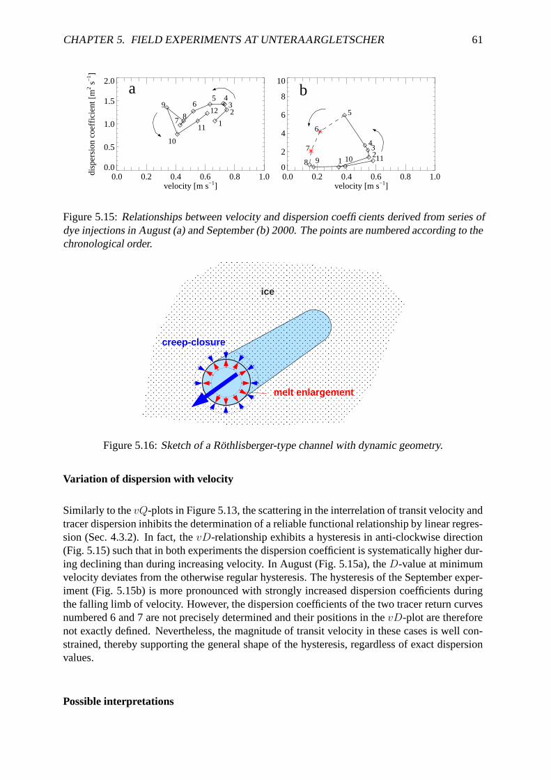
CHAPTER 5. FIELD EXPERIMENTS AT UNTERAARGLETSCHER 61
0.0 0.2 0.4 0.6 0.8 1.0velocity [m s−1]
0
2
4
6
8
10
disp
ersi
on c
oeffi
cien
t [m2 s
−1 ]
1 2 3
4
5
6
7
8 9 10 11
0.0 0.2 0.4 0.6 0.8 1.0velocity [m s−1]
0.0
0.5
1.0
1.5
2.0di
sper
sion
coe
ffici
ent [
m2 s−
1 ]
1
2 3
4 5 6
7 8
9
10
11
12
a b
Figure 5.15: Relationships between velocity and dispersion coefficients derived from series ofdye injections in August (a) and September (b) 2000. The points are numbered according to thechronological order.
ice
melt enlargement
creep-closure
Figure 5.16: Sketch of a Röthlisberger-type channel with dynamic geometry.
Variation of dispersion with velocity
Similarly to the vQ-plots in Figure 5.13, the scattering in the interrelation of transit velocity andtracer dispersion inhibits the determination of a reliable functional relationship by linear regres-sion (Sec. 4.3.2). In fact, the vD-relationship exhibits a hysteresis in anti-clockwise direction(Fig. 5.15) such that in both experiments the dispersion coefficient is systematically higher dur-ing declining than during increasing velocity. In August (Fig. 5.15a), the D-value at minimumvelocity deviates from the otherwise regular hysteresis. The hysteresis of the September exper-iment (Fig. 5.15b) is more pronounced with strongly increased dispersion coefficients duringthe falling limb of velocity. However, the dispersion coefficients of the two tracer return curvesnumbered 6 and 7 are not precisely determined and their positions in the vD-plot are thereforenot exactly defined. Nevertheless, the magnitude of transit velocity in these cases is well con-strained, thereby supporting the general shape of the hysteresis, regardless of exact dispersionvalues.
Possible interpretations

CHAPTER 5. FIELD EXPERIMENTS AT UNTERAARGLETSCHER 62
Dynamic conduit geometry Since the slope of a velocity-discharge relationship reflects di-rectly the hydraulic geometry of the drainage system (Sec. 4.3.1), it seems reasonable to as-sociate the hysteretic behavior of our experiments to an corresponding evolution of the flowpath.
The short transit time of the tracer in the system and its reappearance in a sharp breakthroughcurve suggests flow through an efficient, channelized drainage system. Röthlisberger (1972)postulated channels with a dynamic geometry (Sec. 2.2.2). The size of such a channel is deter-mined by the counteracting processes of melt enlargement due to dissipation of potential energyversus creep-closure of the viscous ice (Fig. 5.16). The consequences of the Röthlisberger-theory for the transit velocity of a tracer is considered in a qualitative model applied to the twoobserved discharge situations. In response to an increasing discharge, a Röthlisberger channelwould be enlarged. On the other hand, when discharge decreases, the water pressure in thechannel would decline. This would cause an enhanced closure rate of the conduit and thereforeresult in a decrease of the channel size. If we compare two channels of different cross-sectionalarea A, both carrying the same discharge Q, the flow velocity v in the larger one would besmaller since continuity requires Q = v A. This mechanism of a Röthlisberger-channel cancoherently explain the decrease of velocity during high discharges in August and September aswell as the subsequent velocity increase at minimum discharge in August. As a further conse-quence, the conduit would be larger on the falling than the rising limb of velocity. To explain theobservation that dispersion is generally larger during declining that during increasing velocity,we conjecture a positive relationship between conduit size and dispersion, because the decreaseof velocity coincides with the enlarged conduit.
Finally, the assumption of an adaptable channel geometry receives additional support by thefact that over the course of one day transit velocities in September were consistently lowerthan those in August although discharge was higher. An increase of the channel diameter asdescribed by the Röthlisberger-theory could permit the drainage of a larger discharge even at alower velocity.
In summary, the ability of a Röthlisberger channel to adjust its size to prevailing hydraulicconditions provides a lucid explanation for the observed hysteretic behavior. However, this hy-pothesis needs to be tested by a quantitative model to investigate whether the physical processescan account for the observed behavior.
Inflow modulation Besides the above interpretation, there is also an alternative explanatoryhypothesis. Figures 5.10 and 5.11 illustrate how transit velocity varies with both the supraglacialand the output discharge during the test series. It is obvious, that the velocity variations weremore closely in phase with Qin than with Qpro. This finding might suggest that the obtainedvelocities are the result of flow through an independent conduit connecting the moulin directlyto the glacier terminus. However, such a scenario is highly implausible since dye emerged inthe outlet stream which carries a much larger discharge than the supraglacial stream enteringthe moulin. Thus, it is clear that the moulin acts as a tributary which joined a main conduitbefore exiting the glacier.
Smart (1990) mentioned “hydraulic damming” due to higher discharge in the main conduitwhich controls the proportion of tracer entering at the junction of tributary and conduit. How-ever, “hydraulic damming” may not be an appropriate term to describe the process since thewater is not blocked at the junction. The pressure conditions in the main channel modulate theinflow from the tributary and we therefore prefer to use the term “inflow modulation”. Fountain
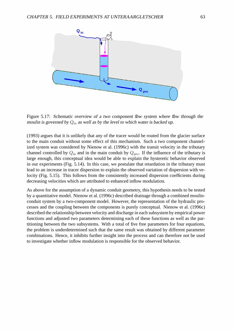
CHAPTER 5. FIELD EXPERIMENTS AT UNTERAARGLETSCHER 63
inQ
proQ
Figure 5.17: Schematic overview of a two component flow system where flow through themoulin is governed by Qin as well as by the level to which water is backed up.
(1993) argues that it is unlikely that any of the tracer would be routed from the glacier surfaceto the main conduit without some effect of this mechanism. Such a two component channel-ized system was considered by Nienow et al. (1996c) with the transit velocity in the tributarychannel controlled by Qin and in the main conduit by Qpro. If the influence of the tributary islarge enough, this conceptual idea would be able to explain the hysteretic behavior observedin our experiments (Fig. 5.14). In this case, we postulate that retardation in the tributary mustlead to an increase in tracer dispersion to explain the observed variation of dispersion with ve-locity (Fig. 5.15). This follows from the consistently increased dispersion coefficients duringdecreasing velocities which are attributed to enhanced inflow modulation.
As above for the assumption of a dynamic conduit geometry, this hypothesis needs to be testedby a quantitative model. Nienow et al. (1996c) described drainage through a combined moulin-conduit system by a two-component model. However, the representation of the hydraulic pro-cesses and the coupling between the components is purely conceptual. Nienow et al. (1996c)described the relationship between velocity and discharge in each subsystem by empirical powerfunctions and adjusted two parameters determining each of these functions as well as the par-titioning between the two subsystems. With a total of five free parameters for four equations,the problem is underdetermined such that the same result was obtained by different parametercombinations. Hence, it inhibits further insight into the process and can therefore not be usedto investigate whether inflow modulation is responsible for the observed behavior.
Chapter 6
Modeling variations of transit velocity
In Chapter 5, it was found that dye injected into a moulin at Unteraargletscher was routedthrough an efficient, channelized drainage system. The observed velocity-discharge relation-ships displayed pronounced hystereses. It was suggested that the dynamic geometry of aRöthlisberger-channel could induce such hystereses. An alternative concept proposes that dis-charge through the moulin might be dammed hydraulically at the junction to a larger conduit,thereby causing the observed behavior.
However, whether conduit evolution happens at a rate fast enough or whether inflow modulationalters the transit time of a tracer sufficiently to explain the observed behavior has to be examinedin detail. This chapter aims to tackle this task by numerical modeling of the proposed mecha-nisms. After a review of existing theories on water flow through subglacial conduits, which gointo more detail than the general considerations in Section 2.2.3, we will introduce a our modelwhich we use to study variations of transit velocity with discharge. We first begin by looking atour visualization of the channelized drainage system beneath Unteraargletscher.
6.1 Visualization of channelized drainage
From the results presented above (Ch. 5), it appears that the investigated flowpath is a subglacialchannel connected to the tributary moulin through which the tracer was injected. Moulins typ-ically descend steeply towards the glacier bed (Holmlund, 1988) where we expect them to joina conduit. As such, we visualize the conduit as located at the glacier bed and incised into theoverlying ice (Fig. 2.3a,b). Similar to the proglacial stream, we conjecture that the bottom of thesubglacial conduit consists of coarse sediments and differently sized blocks. The cross-sectionof the conduit is approximately semi-circular at the terminus of Unteraargletscher but may berather broad and low below the upper part of the glacier where the ice is thicker (Hooke et al.,1990; Cutler, 1998; Ng, 1998). The shape and size of the cross section are determined by the op-posing effects of melt-enlargement due to dissipation of energy and creep-closure due to visco-plastic behavior of the ice-roof (Röthlisberger, 1972). In general, the conduit will principallyfollow the steepest potential gradient (Shreve, 1972). However, in detail, its course is probablynot a direct one but it is most likely meandering and disturbed by intersecting crevasses and theunderlying bedrock relief producing bends and breaks. Similarly, we visualize the distributionof the cross-section along the course of the conduit as irregular, characterized by contractionsand expansions. Since the water exits Unteraargletscher through a single large glacier portal
64

CHAPTER 6. MODELING VARIATIONS OF TRANSIT VELOCITY 65
(Ch. 3.1.3) while meltwater enters the glacier at numerous locations at the surface, it is obviousthat tributary channels join to form a main conduit. Therefore, we believe that the structure ofthe subglacial conduit system is appropriately described by an upglacier branching arborescentnetwork as proposed by Shreve (1972) and Röthlisberger (1972).
6.2 Background
Originally, the theory of conduit flow through a glacier was developed for englacial conduitswhich are completely enclosed by ice. In this case, channelised drainage is a flow of a fluidthrough its solid phase (Spring and Hutter, 1982). The first comprehensive theory was pre-sented by Röthlisberger (1972), who considered an equilibrium state between melt-enlargementand creep-closure. The resulting inverse relationship between water pressure and discharge andits extensive implications for glacial hydrology was already discussed in Section 2.2.3. How-ever, diurnal meltwater input varies on a time scale much shorter than the time needed by such achannel to reach steady-state conditions (Spring, 1980). Therefore, the steady-state assumptionis not appropriate for typical glacier drainage situations. This shortcoming was closed by Nye(1976) who presented a time-dependent theory which he then used to explain the hydrographduring a Jökulhlaup (the Icelandic expression for an outburst of a glacier-dammed lake). Thetheories of Röthlisberger (1972) and Nye (1976) are valid only for straight conduits of circularcross-section that are completely surrounded by ice. Spring (1980) developed therefore a morecomplex and physically based theory for curved and twisted conduits. However, it is strictlyvalid only for conduits which are entirely enclosed by ice since any interaction with the glacierbed is neglected. It was shown by Spring (1980), Spring and Hutter (1981) and Spring and Hut-ter (1982) that the former formulations of Röthlisberger (1972) and Nye (1976) can be derivedas special cases from the more general Spring-theory. Spring (1980) also compared two dif-ferent expressions for frictional head loss: the Manning-Gauckler-Strickler-formula which wasused by Röthlisberger (1972) and Nye (1976) and the Darcy-Weisbach-formula. Differences be-tween the two approaches turned out to be slight and in subsequent studies the Darcy-Weisbachform was adopted (Spring and Hutter, 1982; Kohler, 1995; Clarke, 1996). Where the conduit isin contact with the glacier bed some modifications to the theory have to be made. The frictionbetween ice and bed affects the closure of a conduit in such a way that the inward creep of thebottom ice is retarded with respect to the ceiling of the conduit (Hooke et al., 1990). Hence,its resulting cross-sectional shape is wide and low rather than semi-circular. Further effects arerelated to the interaction between water and glacier bed. As such, the roughness of the bed andthe altered cross-sectional shape would increase the resistance for water flow. This in turn altersthe water pressure gradient thereby affecting the cross-sectional geometry which is additionallychanged by erosion-sedimentation processes of a sedimentary bed. Röthlisberger (1972) arguesthat these alterations to his theory counteract each other and thus, the assumption of a circularcross-section would not introduce much inaccuracy. As mentioned in Section 2.2.3, modifi-cations to the theory were necessary to explain measured water pressures; calculated pressurevalues were consistently too low and agreement could be achieved in two ways. One approachwas the assumption of an enhanced closure-rate (Röthlisberger, 1972; Iken and Bindschadler,1986; Lliboutry, 1983) due to material properties of the basal ice. In a second approach a broadand low cross-sectional geometry is proposed (Hooke, 1984; Hooke et al., 1990). Such a ge-ometry is more resistive to water flow, thereby a higher hydraulic gradient is required to drivethe flow. Additionally, the closure rate of such a broad low cross-section is larger than that ofa semi-circular one. While Hooke et al. (1990) simplified the conduit shape by a segment of

CHAPTER 6. MODELING VARIATIONS OF TRANSIT VELOCITY 66
a circle, the problem of closure of an irregularly shaped cross-section was tackled by Cutler(1998) and Ng (1998). Erosion-sedimentation controlled geometry changes were addressed bythe work of Walder and Fowler (1994) and Ng (2000) yielding equilibrium results contrary tothose of Röthlisberger (1972) for the case of a very thick sediment bed. This case may applyfor ice streams (Alley et al., 1987), but where the sediment layer is thinner, a common situationbeneath alpine glaciers, sediment creep is limited by enhanced strength of sediment in closevicinity to a channel (Alley, 1992). Therefore, channels are likely to become isolated from thedeforming sediment. In this case, the theory for subglacial conduits on a hard bed is againapplicable.
6.3 Model theory
Based on the theories considered above, we now formulate expressions which enable us tosimulate the behavior of a Röthlisberger-channel for given discharge variations. Such a modelshould also allow us to derive a physically based relationship between discharge and flow ve-locity. Since open-channel flow is conceivable in parts of the conduit (Lliboutry, 1983; Hooke,1984; Fountain, 1993; Kohler, 1995; Nienow et al., 1996c), this possibility will be included inthe model as well. Further, aiming for a simulation of our series of tracer experiments, we treatthe problem in a spatially distributed formalism for a simplified geometry of Unteraargletscher.
6.3.1 Assumptions
Despite our visualization of an irregularly meandering subglacial conduit of complex cross-sectional shape and size, the model which will be used for our purpose is rather simple. Thelack of detailed information on the real course and geometry of the conduit requires that wemake the simplest possible assumptions. As such, the following assumptions are included inour model formulation:
1. The conduit is located at the glacier bed and follows the thalweg.
2. The ice is isothermal and at the pressure melting point. This is a typical characteristic ofalpine glaciers. Hence, the energy dissipated by the flow of water is entirely available formelting channel walls.
3. The ice is incompressible and isotropic. Therefore, Glen’s flow law is appropriate todescribe closure-rates.
4. If we consider a uniform distribution of velocity and pressure within the channel cross-section the problem can be reduced to one dimension in flow direction.
5. The contribution to discharge from melting of conduit walls is negligible.
6. The conduit is directed parallel to ice-flow and far-field longitudinal and transverse strain-rates are zero, thus the conduit-axis is stationary.
7. Any thermal energy is produced and consumed locally (within one spatial increment),thus advection of thermal energy into or out of the considered conduit segment is ne-glected.

CHAPTER 6. MODELING VARIATIONS OF TRANSIT VELOCITY 67
8. The conduit has a circular cross-section, i.e. for the computation of closure-rates, wefollow Röthlisberger’s argument (p. 65) and neglect direct influences from the bed. Thissimplifies the matter and the analytical expression for closure-rate of a cylinder (Nye,1953) can be applied.
9. The conduit-axis is straight and effects of curvature, bends and breaks on water flow arenot described explicitly.
10. Any kind of head loss is described by a single friction parameter using the Darcy-Weisbach-formula. In doing so, we have to bear in mind that we omit explicit descriptionsof curvature of the conduit-axis and irregularities of cross-sectional shape and size whichwould cause additional local head losses. Thus, our estimate of the friction parametercomprises frictional as well as local losses.
11. The kinetic potential of the flowing water is small compared to the pressure and topo-graphic potentials and can be neglected.
12. Negative water pressure or suction cannot occur. Instead, water would flow under open-channel conditions and fill the conduit partially. In this case, melting occurs only at thewetted part of the conduit perimeter.
6.3.2 Model equations
The assumptions made above enable us to formulate a simplified model that suits our require-ments.
Energy dissipation
Water flows down a potential gradient ∂H/∂x, with x defining a length in stream-wise direction.Thereby, the water releases potential energy E. The local hydraulic potential is expressed by
H = h + z, (6.1)
where h is water pressure expressed in terms of hydraulic head h = pw/ρwg with pw denotingthe water pressure, ρw the density of water, g the acceleration due to gravity and z is the elevationof the bed relative to a datum. The potential energy released per time t and per unit length dxis given by
∂E
∂t= ρwgQ(t)
∂H
∂xdx. (6.2)
Melt enlargement
This energy is consumed by melting ice at the conduit walls and by maintaining the water atpressure melting conditions. For the considered solid-liquid phase transformation the waterpressure and temperature are inversely correlated, thus, the melting condition requires highertemperature as the pressure drops. The temporal evolution of energy Et required for this processis
∂Et
∂t= ctcwρwQ(t)ρwg
∂h
∂xdx (6.3)

CHAPTER 6. MODELING VARIATIONS OF TRANSIT VELOCITY 68
with ct expressing the change in melting temperature per unit pressure and cw the specific heatof water.
The energy Em required per time step to increase the volume Vm of the conduit by melting iswritten
∂Em
∂t= ρiLf
∂Vm
∂t, (6.4)
where ρi stands for density of ice and Lf for latent heat of fusion. Expressing Vm = Amdx,where Am is the cross-sectional area produced by melting and considering the length of theconduit constant in time (∂x/∂t = 0), we can drop dx from the energy equation E = Em + Et.Solving for ∂Am
∂t, we obtain then
∂Am
∂t=
ρwg
ρiLfQ(t)
(
(1 − γ)∂h
∂x+
∂z
∂x
)
, (6.5)
where γ = ctcwρw defines a dimensionless constant.
Creep-closure
Viscoplastic deformation of ice counteracts the growth of subglacial conduits. Nye (1953)derived an analytical solution for the closure rate of a cylindrical tunnel using Glen’s flow law:
R
R= B
(ρwg
n(h∗
− h))n
. (6.6)
Here, R is the radius of the circular cross-section, the dot indicates derivation with respectto time, B and n are flow law parameters. The ice-overburden pressure expressed in termsof hydraulic head h∗ = ρi/ρwhi is exerted by ice of the thickness hi. Simple geometricalconsiderations reveal Ac = 2πRR, where Ac denotes the cross-sectional area closed by creep.By using Equation (6.6) we obtain
∂Ac
∂t= 2AB
(ρwg
n(h∗
− h))n
(6.7)
where A denotes the cross-sectional area of the conduit. Finally, to derive an equation describ-ing the change of the conduit cross-section with time, we combine the counteracting expressionsfor melt enlargement (Equation (6.5)) and creep closure (Equation (6.7)):
∂A
∂t=
ρwg
ρiLf
Q(t)(
(1 − γ)∂h
∂x+
∂z
∂x
)
− 2AB(ρwg
n(h∗
− h))n
. (6.8)
Pressurized water flow
With an expression relating the release of hydraulic potential ∆H to discharge Q, our modelto describe subglacial drainage is complete. Taking a critical Reynolds-number of about 2300(Weertman, 1972) for water flow through a pipe, it turns out that even for a very small conduitof 0.1 m in diameter a velocity higher than 0.05 m s−1 would cause turbulence. Observationyields typically higher velocities (e.g. Lang et al.,1979; Hock and Hooke, 1993; Nienow, 1993;Fountain, 1993). Hence, flow in subglacial conduits carrying significant water quantities isexpected to be turbulent.

CHAPTER 6. MODELING VARIATIONS OF TRANSIT VELOCITY 69
For turbulent flow through a pipe, the Darcy-Weisbach relation states that:
ρwg∂H
∂x=
fρwv2
8Rh, (6.9)
where v is the mean flow velocity and Rh the hydraulic radius. The dimensionless frictionfactor f depends on the wall-roughness and the Reynolds-number. However, this dependencevanishes for high Reynolds-numbers, hence, for simplicity, we use a constant f . We will jus-tify this assumption a posteriori (Sec. 6.8.2). By definition Rh = Aw/Uw with Aw being thearea occupied by the water and Uw the wetted conduit perimeter. Recalling that the conduit ispressurized yields Aw = A, Uw = U and Q = vA. If solved for Q, Equation (6.9) yields
Q = 2A3/2( 2g
fU
∂H
∂x
)1/2. (6.10)
Open-channel flow
Flow conditions through a conduit are pressurized, where discharge exceeds the maximumamount which can be routed under open-channel flow conditions. This threshold can be de-rived from the Manning-Gauckler-Strickler formula:
v = kR2/3h
(∂z
∂x
)1/2, (6.11)
where k represents a roughness coefficient and water flow is driven by thetopographical potential gradient ∂z/∂x. For a completely filled conduitRh = 1/2 (A/π)1/2 and the corresponding non-pressurized discharge is
Qmax = k(∂z
∂x
)1/22−2/3π−1/3A4/3. (6.12)
We adopt this value as the threshold between pressurized and open-channel flow. Where open-channel flow takes place, the conduit is only partially filled. In this case melt enlargementoccurs only along the wetted perimeter of the conduit. However, we assume that the circularshape of its cross-section persists and consequently the Nye (1953)-solution for creep-closureholds. Thus Equation (6.8) becomes
∂A
∂t= C
ρwg
ρiLf
Q(t)∂z
∂x− 2AB
(ρwg
nh∗
)n, (6.13)
where C = Uw/U is a correction factor that represents the ratio of wetted perimeter Uw to totalperimeter U . For the cross-sectional area occupied by water Aw in a partially filled circularconduit of radius R, the following relation applies:
Aw =R2
2
(
α − sin α) (6.14)
where the angle α is defined as shown in Figure 6.1. From the simple continuity relation Q =vAw, Equation (6.11) and the definition of Rh = Aw/Uw we obtain
Q = k(∂z
∂x
)1/2U−2/3
w A5/3w . (6.15)

CHAPTER 6. MODELING VARIATIONS OF TRANSIT VELOCITY 70
R
α
Uw
Aw
Figure 6.1: Cross-section of a partly-filled circular conduit. The shaded area represents the areaoccupied by the water, Aw.
Substituting Equation (6.14) and α = Uw/R yields
Q3/5k−3/5(∂z
∂x
)
−3/10 2
R2= U−2/5
w
(Uw
R− sin
Uw
R
)
. (6.16)
This equation cannot be solved analytically for Uw. Figure 6.2 illustrates that the relation ofdischarge and filling depth in a partly filled circular conduit is not unique for high filling levels.At such a high filling level, Uw increases faster with filling depth than Aw. In consequence, whenwater fills the conduit to 92%, a slightly larger discharge is drained than that at higher fillinglevels. This point marks the transition to pressurized flow when the filling depth in a partly filledconduit increases. In contrast, the transition from pressurized to open-channel flow takes placeat a discharge which corresponds to complete filling (Chow, 1988; Hager, 1995). We recallthat we treat this transition by a single value Qmax (Equation (6.12)) instead of two differentthresholds for opening and closing. However, the resulting error in the calculated pressures isof the order of 10−5m for typical values of A (5–10 m2). We neglect this inaccuracy because itis small compared to typical hydraulic head variations which are of the order of several meters.
The value of Uw was iterated by finding the zero of an objective function ε = X − Y , whereX stands for the left hand side and Y for the right hand side of Equation (6.16). Ambiguoussolutions where avoided by starting the approximation of Uw from zero. In doing so, we willalways approach the physical meaningful solution first.
Computation of flow velocity
When the water flow through the conduit is pressurized, mean flow velocity can easily be ob-tained from
v =Q
A. (6.17)
To determine v in the case of open-channel flow, A in Equation (6.17) has to be replaced by Aw.Once Uw is determined, Aw follows from Equation (6.14) using α = Uw/R.

CHAPTER 6. MODELING VARIATIONS OF TRANSIT VELOCITY 71
0.0 0.2 0.4 0.6 0.8 1.0 1.2rel. discharge
0.0
0.2
0.4
0.6
0.8
1.0
rel.
dept
h
Figure 6.2: The discharge through a partly filled circular conduit as a function of filling depth.The values are normalized with respect to those that correspond to complete filling.
6.4 Model implementation
6.4.1 Flow resistors
So far, we derived expressions describing water flow and the evolution of the conduit geome-try. To integrate these equations we formulate a scheme for numerical computation. For thispurpose, we follow the formulation of Clarke (1996) defining a hydraulic analogue to Ohm’slaw in electricity for both linear as well as nonlinear flow resistances. Water discharge is drivenby the release of hydraulic potential ∆H through a hydraulic system exerting a resistance to-wards flow. The passage of water is obstructed by friction on the system boundaries, thus, theresistance is governed by roughness elements, the geometry of the system and the type of flow.Linear resistance RL is characterized by a H-Q-relationship:
∆H = QRL (6.18)
and is associated with laminar flow. In contrast, turbulent flow obeys power-law relations of theform:
∆H = Q2FT, (6.19)
with FT denoting a resistance parameter. We may define a nonlinear resistance that increaseslinearly with discharge RT = QFT and consequently we obtain:
∆H = QRT. (6.20)
Using this formalism, expressing Q by Equation (6.10) and using U = 2(πA)1/2 (since weconsider a circular cross-section) yields
RT =π1/4
2A5/4
(f ∆x ∆H
g
)1/2. (6.21)
In contrast to a linear resistor RL which is a function of geometry only, a turbulent resistorRT depends on geometry, roughness and the applied hydraulic potential difference ∆H and istherefore nonlinear.

CHAPTER 6. MODELING VARIATIONS OF TRANSIT VELOCITY 72
It is useful to consider an element of a fixed length ∆x. All spatially dependent processes areassumed to be constant on this length scale. This implies that the potential gradient ∆H/∆xand the conduit cross-section A are constant along the element and consequently, the partialdifferential Equations (6.8) and (6.10) become ordinary.
Finally, we obtain the equations describing turbulent flow through a Röthlisberger-channel,represented by an element with resistance RR. This system is described by Equations (6.20)
∆H = QRR
and Equation (6.21)
RR =π1/4
2A5/4
(f ∆x ∆H
g
)1/2
combined with Equation (6.8) if flow is pressurized
dA
dt=
ρwg
ρiLfQ(t)
(
(1 − γ)∆h
∆x+
∆z
∆x
)
− 2AB(ρwg
n(h∗
− h))n
.
For open-channel flow the system is determined by
∆H = ∆z
and Equation (6.13)dA
dt= C
ρwg
ρiLfQ(t)
∆z
∆x− 2AB
(ρwg
nh∗
)n.
In the latter case, we omit the explicit expression for the resistance of an open conduit since thecalculation of H is trivial with h = 0.
This formulation is consistent with Clarke’s (1996), except for the hydraulic potential whichis used here as the driving force instead of hydraulic head, enabling us to consider inclinedconduits.
6.4.2 Numerical scheme
In this section, we aim to model variations of transit velocity due to changing hydraulic condi-tions along the flow path. This is achieved by investigating the water pressure distribution alonga R-channel in response to a given discharge. The approach requires a linear arrangement offlow resistors to obtain the desired longitudinal resolution by considering the topographies ofglacier surface and glacier bed. In discretized form, the system of equations describing turbu-lent flow through a Röthlisberger-channel contains i algebraic equations describing the drop ofhydraulic head over a spatial increment ∆x:
hi − hi−1 = (zi−1 − zi) + Q2 π1/2f ∆x
4gA5/2i
(6.22-a)
if flow is pressurized, otherwisehi = 0 (6.22-b)
and i ordinary differential equations describing the temporal evolution of the conduit cross-section. For pressurized flow
dAi
dt=
ρwg
ρiLfQ(t)
(
(1 − γ)(∆h
∆x
)
i+(∆z
∆x
)
i
)
− 2AiB(ρwg
n(h∗
i − hi))n
(6.23-a)

CHAPTER 6. MODELING VARIATIONS OF TRANSIT VELOCITY 73
derivative: v(t)
initial conditions:steady state profiles of
h and A
glacier geometry:profiles of h* and z
input:Q(t)
for each ∆x and ∆t:
Q ≥ Q max ?
no: open-channel flow→ iterate Uw in eq. 6.16 and solve eq. 6.22b and 6.23b
output:profiles of h(t) and A(t)
yes: pressurized flow
→ solve eq. 6.22a and 6.23a
Figure 6.3: Outline of the modeling procedure.
and under open-channel conditions
dAi
dt= C
ρwg
ρiLfQ(t)
(∆z
∆x
)
i− 2AiB
(ρwg
nh∗
)n(6.23-b)
The glacier geometry in terms of bed elevation z and ice-overburden pressure h∗ has to beprescribed as well as initial conditions for the distribution of hydraulic head h and conduitcross-sectional area A. Furthermore, one of the model boundaries requires a constraint fromwhere the integration is started. Then, with a given discharge Q, the system of equations issolved for each spatial and temporal increment. From the resulting distributions of h and A,we derive the transit velocity of water v. The procedure of the model calculation is outlined inFigure 6.3.
In this study, we have implemented our model using Clarke’s (1996) program code which solvessimilar equations. A problematic feature of this system of equations is its hybrid compositionof both differential and algebraic equations (Hairer et al., 1995). This demands the employmentof specially designed numerical methods to compute solutions. Here, the public domain solverddriv3 was used, an elaboration of the program sdriv2 described by Kahaner et al. (1989).Special attention is required by the fact that the governing equations prove to be numericallystiff. An obvious source of stiffness is introduced by nonlinearities such as in Equation (6.23-a)near Q = Qmax. A further source of stiffness is related to the interaction of differential andalgebraic equations. An algebraic relation e.g. a = b/c can equivalently be expressed as adifferential equation ε da/dt = b/c− a, where ε is an infinitesimally small time constant. Suchcoexistence of very small and large time constants in the same system is a characteristic ofstiffness. Additionally, special caution is required for an accurate choice of initial conditions.

CHAPTER 6. MODELING VARIATIONS OF TRANSIT VELOCITY 74
Table 6.1: Physical constants
Physical property Value Unit
Gravity acceleration g 9.8 m s−2
Density of ice ρi 900 kg m−3
Density of water ρw 1000 kg m−3
Latent heat of melting Lf 333.5 kJ kg−1
Pressure melting coefficient ct −7.4 × 10⁻⁸ K J−1 m3
Specific heat of water cw 4.22 × 10³ J kg−1 K−1
A physically implausible initial state is very likely to cause a prompt failure of the numericalintegration. Here, we assumed that the system is initially in steady-state. In most applications,we used the boundary condition h = 0 for x = 0 in accordance with the observation thatthe water is leaving Unteraargletscher at atmospheric pressure. Then, the initial conditions forAi and hi can be calculated using the analytical solution for a stationary discharge through aR-channel as derived by Röthlisberger (1972).
6.5 Behavior of the model
6.5.1 Validation of steady-state profile
In a first application we examine the performance of our model and possible constraints for itsspatial discretization. Röthlisberger (1972) derived an analytical solution for his steady-statetheory by assuming stationary discharge in a horizontal conduit beneath ice of uniform thick-ness. By balancing the rates of melt-enlargement and creep-closure of an horizontal conduit,he obtained an expression for the hydraulic head gradient (Röthlisberger, 1972, equation (8)),which in our notation corresponds to
dh
dx= 2AB
Lfρi
(1 − γ)Q−1(ρwg)n−1
(
h∗ − h
n
)n
. (6.24)
However, he used the Manning-Gaukler-Strickler formula (Equation (6.11)) to eliminate Awhereas we adopted the Darcy-Weisbach relation (Equation (6.9)). We repeated Röthlisberger’sderivation to obtain the corresponding steady-state solution
h(x) = h∗−
(
(
2πB5(
Lfρi
1 − γ
)5
(ρwgn)7−5n f 2
g2Q−1
)1
7 5n − 7
7x + h∗
7−5n
7
)7
7−5n
. (6.25)
This expression was used to validate the model performance. The physical constants used inthe computations are listed in Table 6.1. Further, it is assumed that the friction factor f aswell as the material properties of ice, expressed as n and B, are constant along the conduit.Values used for these model parameters are presented in Table 6.2. Flow law parameters wereadopted from Nye (1953) and the choice for f follows Spring and Hutter (1982). The value ofk was determined by trial and error to achieve agreement of Röthlisberger’s solution with oursteady-state solution (Equation (6.25)). The values of f and k are within the narrow range ofroughness coefficients which were determined for subglacial conduits by other authors (Nye,
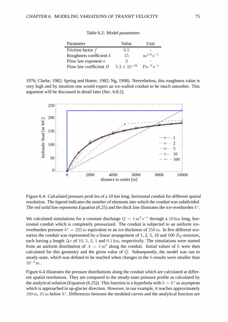
CHAPTER 6. MODELING VARIATIONS OF TRANSIT VELOCITY 75
Table 6.2: Model parameters
Parameter Value Unit
Friction factor f 0.5 -Roughness coefficient k 15 m1/3 s−1
Flow law exponent n 3 -Flow law coefficient B 5.3 × 10⁻²⁴ Pa−3 s−1
1976; Clarke, 1982; Spring and Hutter, 1982; Ng, 1998). Nevertheless, this roughness value isvery high and by intuition one would expect an ice-walled conduit to be much smoother. Thisargument will be discussed in detail later (Sec. 6.8.2).
0 2000 4000 6000 8000 10000distance to outlet [m]
0
50
100
150
200
250
hydr
aulic
hea
d [m
WC
]
12510100
Figure 6.4: Calculated pressure profiles of a 10 km long, horizontal conduit for different spatialresolution. The legend indicates the number of elements into which the conduit was subdivided.The red solid line represents Equation (6.25) and the thick line illustrates the ice-overburden h∗.
We calculated simulations for a constant discharge Q = 1 m3 s−1 through a 10 km long, hor-izontal conduit which is completely pressurized. The conduit is subjected to an uniform ice-overburden pressure h∗ = 225 m equivalent to an ice-thickness of 250 m. In five different sce-narios the conduit was represented by a linear arrangement of 1, 2, 5, 10 and 100 RR-resistors,each having a length ∆x of 10, 5, 2, 1 and 0.1 km, respectively. The simulations were startedfrom an uniform distribution of A = 1 m2 along the conduit. Initial values of h were thencalculated for this geometry and the given value of Q. Subsequently, the model was run tosteady-state, which was defined to be reached when changes in the h-results were smaller than10−4 m .
Figure 6.4 illustrates the pressure distributions along the conduit which are calculated at differ-ent spatial resolutions. They are compared to the steady-state pressure profile as calculated bythe analytical solution (Equation (6.25)). This function is a hyperbola with h = h∗ as asymptotewhich is approached in up-glacier direction. However, in our example, it reaches approximately180 m, 45 m below h∗. Differences between the modeled curves and the analytical function are

CHAPTER 6. MODELING VARIATIONS OF TRANSIT VELOCITY 76
systematically positive. In general, the accuracy of the model increases with increasing spa-tial resolution. When the conduit is represented by a single, 10 km long resistor, the waterpressure 10 km from the outlet approaches the ice-overburden pressure, thereby exceeding thesteady-state value by about 45 m. The values calculated by the two-resistor scenario deviate by∼10−15 m whereas a ∆x of 2 km reproduces the analytical solution well. A choice of less than1 km for ∆x appears to be appropriate to mirror the analytically derived steady-state profile.
6.5.2 Response to discharge variations of different periods
Further simulations were undertaken with the same model geometry, representing a horizontalconduit under a uniformly thick glacier. The 5 km long conduit was subdivided into 50 RR-resistors of 0.1 km length each. Now, we focused on the time-dependent pressure responsewhen the conduit was exposed to a sinusoidal discharge function Q(t):
Q(t) =Qup − Qlow
2( − cos(ωt)) +
Qup + Qlow
2, (6.26)
where ω = 2π/T denotes the angular velocity corresponding to the period T . The limits Qup
and Qlow were chosen such that Q(t) describes a sine between 1 and 6 m3 s−1.
Probably the most essential statement of Röthlisberger’s steady-state theory is the prediction ofan inverse relationship between discharge and pressure (cf. Equation (6.25)). In contrast, forflow through a rigid pipe, the relationship would be a direct one (Equation (6.9)). Consequently,the behavior of a R-channel would be somewhere between these two end members, dependingon the state to which the conduit has developed and how close this state is from equilibriumconditions. To illuminate the phase-relationship between Q(t) and h(t), we have produced aset of eight scenarios by adopting the values 1, 2, 5, 10, 25, 50, 100 and 500 d for the period Tof the discharge variation Q(t).
Figure 6.5 presents three examples of the resulting h(t)-variations in response to a sinusoidalQ(t)-input with different periods. To illustrate the course of h(t), we present the pressurecalculated for the location at 5 km distance from the terminus. Therefore, the absolute values atany other point in the conduit differ from those presented here. However, the temporal behavioris identical at any arbitrary distance.
The strong dependence of the h(t)-variations on the period T is evident. For T = 1 d, thevariations of discharge and pressure are almost in phase, whereas for T = 10 d and T = 100 dthe phase shift between peak discharge and maximum pressure increases to 0.4π and 0.67π,respectively.
The pressure regimes of these three scenarios differ substantially from each other. In the T =1 d case, the h-curve is almost symmetrical whereas with increasing T the shape becomes moreasymmetrical such that in the T = 100 d-scenario, the curve is characterized by a steep rise anda gently declining tail. Similarly, the magnitude of the h-variation is dependent on T as well.To drive the diurnally cycling discharge in our example through the conduit, a hydraulic headranging between 12 and 422 m is required. At longer periods, the minimum pressure increasessimultaneously with a reduction of the maximum such that the amplitude decreases.
Furthermore, Figure 6.5 presents also the evolution of the cross-sectional area A at 5 km dis-tance from the terminus for the three considered cases. In the T = 1 d-scenario, A varies

CHAPTER 6. MODELING VARIATIONS OF TRANSIT VELOCITY 77
0.2 0.4 0.6 0.8 1.0time [d]
0
2
4
6
8
disc
harg
e [m
3 s−
1 ]
0
100
200
300
400
500
head
[m W
C]
0
2
4
6
cros
s−se
ctio
nal a
rea
[m2 ]
T = 1d QhA
2 4 6 8 10time [d]
0
2
4
6
8
disc
harg
e [m
3 s−
1 ]
0
200
400
head
[m W
C]
0
2
4
6
cros
s−se
ctio
nal a
rea
[m2 ]
T = 10d QhA
20 40 60 80 100time [d]
0
2
4
6
8
disc
harg
e [m
3 s−
1 ]
100
120
140
160
180
200
head
[m W
C]
0
2
4
6cr
oss−
sect
iona
l are
a [m2 ]
T = 100d QhA
Figure 6.5: Variations of pressure h (dashed) in a R-channel at 5 km distance from the terminusin response to a sinusoidal discharge input Q (dashed). The corresponding evolution of thecross-sectional area A is shown by the dotted line. The periods of the discharge function are1 day (top), 10 days (center) and 100 days (bottom). Note that the pressure-axes are scaleddifferently.
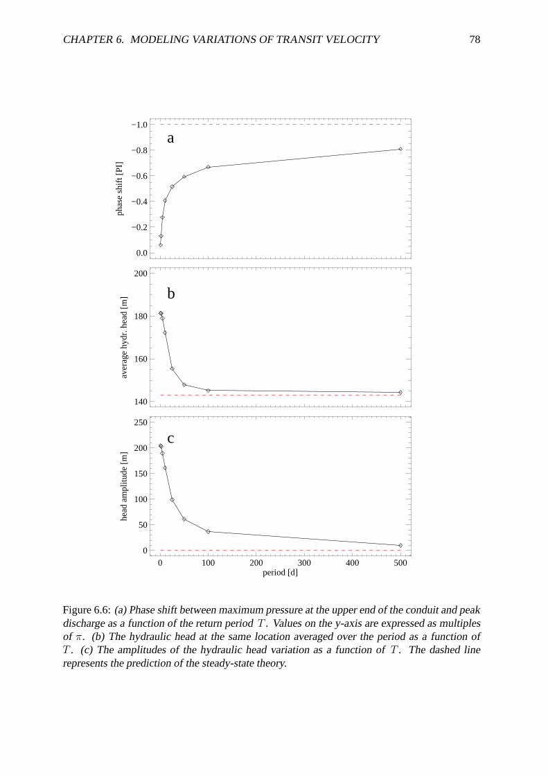
CHAPTER 6. MODELING VARIATIONS OF TRANSIT VELOCITY 78
0 100 200 300 400 500period [d]
0.0
−0.2
−0.4
−0.6
−0.8
−1.0ph
ase
shift
[PI]
0 100 200 300 400 500period [d]
140
160
180
200
aver
age
hydr
. hea
d [m
]
0 100 200 300 400 500period [d]
0
50
100
150
200
250
head
am
plitu
de [
m]
a
b
c
Figure 6.6: (a) Phase shift between maximum pressure at the upper end of the conduit and peakdischarge as a function of the return period T . Values on the y-axis are expressed as multiplesof π. (b) The hydraulic head at the same location averaged over the period as a function ofT . (c) The amplitudes of the hydraulic head variation as a function of T . The dashed linerepresents the prediction of the steady-state theory.

CHAPTER 6. MODELING VARIATIONS OF TRANSIT VELOCITY 79
only slightly around a value of roughly 3 m2 and the variation follows the course of Q with aphase-shift of 0.5π. Towards longer periods of the Q-regime, the amplitude of the A-variationincreases while the time lag by which it follows Q, decreases. As such, for T = 10 d, A varieswith an amplitude of ∼0.9 m2 and a phase-shift of 0.4π with respect to Q, while for T = 100 d,the corresponding values are 1.87 m2 and 0.1π, respectively.
This unequal evolution of the cross-sectional area for different periods of the discharge varia-tion is responsible for the observed hydraulic head regime. Whereas for fast Q-variations, theconduit size cannot respond fast enough to reach a steady-state, a slowly changing dischargepermits almost complete adjustment of the conduit cross-section to prevailing hydraulic condi-tions.
These findings are illustrated in Figures 6.6a–c where the phase shift, average pressure andpressure amplitude are presented as a function of the period T . Further, we compare theseresults with the values obtained from applying Equation (6.25) to the average discharge input.
Figure 6.6a shows how the phase shift increases with T . As mentioned, for small values ofT , the phase shift is close to zero but increases quickly such that a value of 0.5π is reached atT ≈ 20 d. However, the anti-phase behavior predicted by the steady state theory is not reachedin our scenarios not even for T = 500 d.
The pressures averaged over the period (Fig. 6.6b) decrease quickly from about 180 m at T =1 d to approximately 145 m at T = 100 d close to the steady-state value of 143 m. For T >100 d, the decline is very weak.
A similar picture emerges for the magnitudes of the pressure amplitude (Fig. 6.6c). From T =1 d to T = 100 d, the amplitude reduces by a factor of five. The decline attenuates towardslonger periods and approaches the steady-state value at T ≈ 500 d.
6.6 Model applications
6.6.1 Variations of velocity in a subglacial channel
To test the hypothesis, that changes of the conduit size can account for the observed vQ-hysteresis (Sec. 5.4.3), we applied the model to a geometry representing Unteraargletscher.With several distinct model scenarios we attempted to simulate situations as observed in thefield.
The straight-line distance from the moulin where the tracer was injected to the glacier terminuswhere it was detected is approximately 4.5 km. We assume, that the water is transfered from thesurface directly into a main R-channel which carries the bulk of runoff from Unteraargletscherto the glacier portal. Further, it is assumed that this conduit follows the thalweg of the glacierbed. The conduit has then a length of approximately 5 km.
In our calculation, the conduit was represented by a linear arrangement of 100 RR-resistorsof 50 m length each. The glacier geometry was imported into the model by adopting localvalues of the bed slope ∆z/∆x and the ice-overburden h∗. Since the glacier bed below thetongue of Unteraargletscher is steadily inclined, a single, constant value of ∆z/∆x = 0.012

CHAPTER 6. MODELING VARIATIONS OF TRANSIT VELOCITY 80
0 1000 2000 3000 4000 5000distance from terminus [m]
0
100
200
300
400
500
elev
atio
n [m
]
02
4
6
810
cros
s−se
ctio
nal a
rea
[m2 ]
b
a
Figure 6.7: (a) Longitudinal profile of conduit cross-sectional area determined for the Unter-aargletscher geometry and a constant discharge Q = 10.75 m3 s−1. (b) Longitudinal profilesof steady-state water pressure (dashed), the glacier bed (dotted) and the overburden-pressureexerted by the ice (solid).
was estimated from Figure 1.2. In a similar way, a profile of ice-thickness along the centerlineof Unteraargletscher was derived and represented by a parabolic function:
h∗(x) = −8.44 × 10−6x2 + 0.1082x − 1.07. (6.27)
To study the behavior of such a conduit under typical drainage conditions, diurnal discharge cy-cles were prescribed by a sine function varying between 9 and 12.5 m3 s−1. As initial conditionfor the conduit cross-sectional area, the steady-state geometry for a constant average discharge,Q = 10.75 m3 s−1 was derived similar as described in Section 6.5.1. The longitudinal profile ofthis steady-state geometry is shown in Figure 6.7a. In the upper part of the conduit, the cross-sectional area is about 5 m2 but increases up to ∼8 m towards the terminus where the glacierthins out, thereby reducing the closure rate. Figure 6.7b illustrates the distribution of bed eleva-tion and ice overburden-pressure which were used in our calculations as well as the distributionof steady-state water pressure in the conduit which served to start the calculations.
Subsequently, we calculated variations of pressure and velocity along the channel. Thereforewe implemented two fundamentally different approaches. In a first scenario, we considered aconduit with a static cross-sectional geometry as employed e.g. by Fountain (1993) and Kohler(1995) for a comparable purpose. In the remainder of this study, this channel geometry will bereferred to as the “rigid pipe”. Implementation of this pipe into the model was achieved by de-scribing the equations for a corresponding resistor RP. This requires only minor changes of theexpressions described above. Since we consider identical mechanisms of water flow, the Equa-tions (6.22-a, b) remain unchanged and the static nature of the pipe is accounted for by removingthe differential equation expressing the evolution of the conduit size A (Equations (6.23-a, b)).

CHAPTER 6. MODELING VARIATIONS OF TRANSIT VELOCITY 81
h
inQ
outQ
subQ
maxh
Qconduit
Figure 6.8: Sketch of the moulin-model configuration.
The second scenario was performed considering the full complexity of the model as describedby the system of Equations (6.22) and (6.23). In this case, water flows through an inclinedR-channel whose geometry adjusts to hydraulic conditions by the counteracting processes ofmelt-enlargement and creep-closure (Röthlisberger, 1972; Nye, 1976).
Further, the flow regime in both scenarios is hybrid. That means that both pressurized as wellas open-channel flow occurs, depending on whether the discharge of water is sufficient to fillthe conduit cross-section or not. This switching condition is examined by Equation (6.12).
6.6.2 Retardation in a tributary moulin
Retardation of water in a tributary due to inflow modulation at the junction to a main conduitcould provide an alternative possibility to explain the observed vQ-hysteresis (Sec. 5.4.3). Us-ing an appropriate model, we would like to test whether the proposed mechanism could explainthe observed vQ-hysteresis.
We recall that in our tracer experiments, the dye was injected into a supraglacial stream atits entrance into a moulin. A moulin that joins a major conduit might act as a piezometerreflecting thereby the water pressure in the conduit. To consider the transit of a tracer throughthe combined moulin-conduit system, we describe this situation by a moulin at a certain distancefrom the terminus which connects subglacially into a conduit (Fig. 5.17).
Now we review this mechanism to derive an adequate formulation of the model. Figure 6.8illustrates the configuration of the model and its individual components. Where a moulin joinsa pressurized channel carrying a subglacial discharge Qsub, water backs up in the moulin to acertain hydraulic head hmoulin. This hydraulic head determines the discharge Qconduit which isrouted through the conduit having a resistance Rconduit and hence Qconduit = hmoulin/Rconduit.The water to build up hmoulin is obtained from the surface input into the moulin Qin and partlyfrom upwelling of excess discharge of Qsub which cannot be driven through Rconduit. Consid-ering the water balance of the moulin, we can derive the following equation to describe thetemporal evolution of hmoulin:
dhmoulin
dt=
0 : hmoulin ≥ hmax, Qin ≥ Qout
0 : hmoulin ≤ 0, Qin ≤ QoutQin−Qout
Amoulin
: otherwise,(6.28)
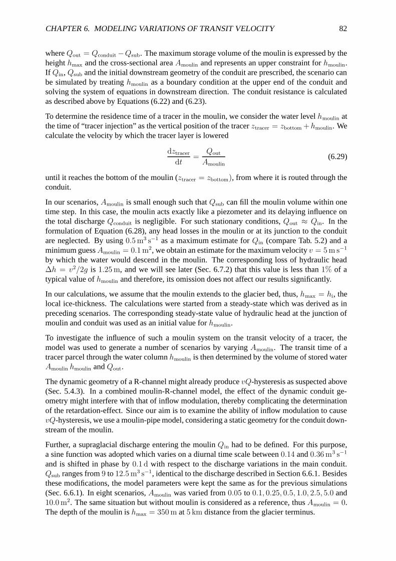
CHAPTER 6. MODELING VARIATIONS OF TRANSIT VELOCITY 82
where Qout = Qconduit −Qsub. The maximum storage volume of the moulin is expressed by theheight hmax and the cross-sectional area Amoulin and represents an upper constraint for hmoulin.If Qin, Qsub and the initial downstream geometry of the conduit are prescribed, the scenario canbe simulated by treating hmoulin as a boundary condition at the upper end of the conduit andsolving the system of equations in downstream direction. The conduit resistance is calculatedas described above by Equations (6.22) and (6.23).
To determine the residence time of a tracer in the moulin, we consider the water level hmoulin atthe time of “tracer injection” as the vertical position of the tracer ztracer = zbottom +hmoulin. Wecalculate the velocity by which the tracer layer is lowered
dztracer
dt=
Qout
Amoulin(6.29)
until it reaches the bottom of the moulin (ztracer = zbottom), from where it is routed through theconduit.
In our scenarios, Amoulin is small enough such that Qsub can fill the moulin volume within onetime step. In this case, the moulin acts exactly like a piezometer and its delaying influence onthe total discharge Qconduit is negligible. For such stationary conditions, Qout ≈ Qin. In theformulation of Equation (6.28), any head losses in the moulin or at its junction to the conduitare neglected. By using 0.5 m3 s−1 as a maximum estimate for Qin (compare Tab. 5.2) and aminimum guess Amoulin = 0.1 m2, we obtain an estimate for the maximum velocity v = 5 m s−1
by which the water would descend in the moulin. The corresponding loss of hydraulic head∆h = v2/2g is 1.25 m, and we will see later (Sec. 6.7.2) that this value is less than 1% of atypical value of hmoulin and therefore, its omission does not affect our results significantly.
In our calculations, we assume that the moulin extends to the glacier bed, thus, hmax = hi, thelocal ice-thickness. The calculations were started from a steady-state which was derived as inpreceding scenarios. The corresponding steady-state value of hydraulic head at the junction ofmoulin and conduit was used as an initial value for hmoulin.
To investigate the influence of such a moulin system on the transit velocity of a tracer, themodel was used to generate a number of scenarios by varying Amoulin. The transit time of atracer parcel through the water column hmoulin is then determined by the volume of stored waterAmoulin hmoulin and Qout.
The dynamic geometry of a R-channel might already produce vQ-hysteresis as suspected above(Sec. 5.4.3). In a combined moulin-R-channel model, the effect of the dynamic conduit ge-ometry might interfere with that of inflow modulation, thereby complicating the determinationof the retardation-effect. Since our aim is to examine the ability of inflow modulation to causevQ-hysteresis, we use a moulin-pipe model, considering a static geometry for the conduit down-stream of the moulin.
Further, a supraglacial discharge entering the moulin Qin had to be defined. For this purpose,a sine function was adopted which varies on a diurnal time scale between 0.14 and 0.36 m3 s−1
and is shifted in phase by 0.1 d with respect to the discharge variations in the main conduit.Qsub ranges from 9 to 12.5 m3 s−1, identical to the discharge described in Section 6.6.1. Besidesthese modifications, the model parameters were kept the same as for the previous simulations(Sec. 6.6.1). In eight scenarios, Amoulin was varied from 0.05 to 0.1, 0.25, 0.5, 1.0, 2.5, 5.0 and10.0 m2. The same situation but without moulin is considered as a reference, thus Amoulin = 0.The depth of the moulin is hmax = 350 m at 5 km distance from the glacier terminus.

CHAPTER 6. MODELING VARIATIONS OF TRANSIT VELOCITY 83
6.7 Results
6.7.1 Variations of velocity in a subglacial channel
Rigid pipe
The transit velocity as determined by a tracer test represents an average over the length ofthe flowpath. Similarly, we have calculated average values of modeled velocities along thepipe for each time step. Figure 6.9a illustrates the phase relations between discharge Q, meanvelocity v and hydraulic head h for water flowing through a rigid pipe with dimensions shown inFigure 6.7. Pressure head h and cross-sectional area A are those calculated at a distance of 5 kmfrom the terminus. The hydraulic head in response to the applied discharge varies sinusoidallybetween ∼85 and ∼215 m and is exactly in phase with Q. This behavior is expected when webear in mind the static geometry of the pipe. Since v is derived from Q, h and A, it followsthe course of Q (and that of h) since A remains constant. The resulting velocity ranges fromapproximately 1.75 m s−1 during the discharge minimum to 2.2 m s−1 at peak discharge.
The distributions of hydraulic potential along the pipe in response to the discharge variationsare presented in Figure 6.9b. Along a pipe of constant cross-section, the hydraulic head woulddecrease linearly from the upper end of the pipe to zero at the point where the flow regimeswitches to open-channel flow. However, since we considered a pipe with diameter that in-creases towards the glacier terminus (Fig. 6.7), the resulting pressure distribution is not linear.In the upper part of the pipe the head loss is approximately linear but it gradually approachesthe shallower bed gradient in the lower part where open-channel flow occurs. During peak dis-charge, open-channel flow occurs in the lowermost 200 m of the pipe while it extends to thelowermost 1000 m during minimal discharge.
The resulting velocity profiles underline the hybrid nature of the flow regime (Fig. 6.9c). In thefreely draining lower part of the pipe, the velocity depends mainly on the bed slope and onlyweakly on the hydraulic radius (Equation (6.11)). Therefore, v is almost constant. A noticeablejump marks the transition to pressurized flow. The transition from open-channel to pressurizedflow occurs not steadily but the water level in a partly filled conduit cross-section switchessuddenly to complete filling when the critical discharge Qmax is reached (Fig. 6.2). As such,the cross-sectional area which is occupied by water Aw is suddenly increased and consideringthe same discharge, continuity requires that the velocity drops at the transition. Where thewater flow is pressurized, the velocity reflects directly the pressure gradient. Hence, initially,values increase steeply. Subsequently, the rise weakens gradually until a maximum is reached atapproximately 3.8 km from the glacier terminus. From there, the velocity decreases slightly toreach a constant value. The differences between maximum and minimum velocities at a givensite scale with the diurnal amplitude of hydraulic head and range from ∼0.1 m s−1 at the outletto ∼0.7 m s−1 at 5 km distance from the terminus.
In consequence of the fact that velocity varies exactly in phase with discharge through a rigidpipe, the velocity-discharge relationship shown in Figure 6.10 is univocal. Since we considereda hybrid system where pressurized as well as open-channel flow occurred, the resulting vQ-curve is slightly bent but this effect is almost not perceptible here. The appearance of the curvein terms of slope and curvature is determined by the cross-sectional size of the drainage systemand the partitioning between distinct types of flow (Fountain, 1993; Kohler, 1995). However,since drainage through a rigid pipe cannot account for the observed vQ-hysteresis, we do notfurther pursue this drainage configuration.

CHAPTER 6. MODELING VARIATIONS OF TRANSIT VELOCITY 84
0.0 0.2 0.4 0.6 0.8 1.0time [d]
8
9
10
11
12
13
14di
scha
rge
[m3 s
−1 ]
1.8
2.0
2.2
velo
city
[m s−
1 ]
100
150
200
hydr
aulic
hea
d [m
]
4.60
4.70
4.80
4.90
5.00
cros
s−se
ctio
nal a
rea
[m2 ]QvhA
0 1000 2000 3000 4000 5000distance from terminus [m]
0
100
200
300
400
500
elev
atio
n [m
]
0 1000 2000 3000 4000 5000distance from terminus [m]
1.5
2.0
2.5
velo
city
[m s−
1 ]
a
b
c
Figure 6.9: (a) Diurnal cycles of discharge Q, mean flow velocity v, hydraulic head h andcross-sectional area A calculated for a rigid pipe. The plot shows h and A at a distance of 5km from the terminus. (b) Longitudinal profiles of glacier bed (shaded), glacier surface (solid)and hydraulic potential (dashed). The range of hydraulic potential is illustrated by the profilesat maximum (upper profile) and minimum (lower profile) discharge. (c) Distribution of flowvelocity along the rigid pipe. The two situations correspond to maximum (upper profile) andminimum (lower profile) discharge.

CHAPTER 6. MODELING VARIATIONS OF TRANSIT VELOCITY 85
9 10 11 12 13discharge [m3 s−1]
1.8
2.0
2.2
velo
city
[m s−
1 ]
Figure 6.10: Velocity-discharge relationship derived from modeled drainage through a rigidpipe.
R-channel
Results obtained from modeling drainage through an inclined, hybrid R-channel are presentedin the same way as for the previous scenario. Figure 6.11 shows phase relations between indi-vidual variables and distributions of both the hydraulic potential and the resulting flow velocityalong the conduit. In general, findings are similar in shape and magnitude to those of the firstscenario. However, the key differences arise from the dynamic nature of the conduit cross-section. Figure 6.11a illustrates the variation of the cross-sectional area A around the steady-state size of ∼4.8 m. The evolution of the cross-sectional area A responds to the discharge cyclewith a delay of ∼6 h. This time lag causes also a phase shift between Q and h. During risingdischarge, the conduit cross-section is smaller than at the falling limb of Q and thus, a lowerhydraulic head is required to drive the same discharge. Therefore, maximum pressure precedespeak discharge by about 1.2 h causing thereby also a comparable phase shift between velocityand discharge. The pressure distributions along the channel in Figure 6.11b resemble very muchthose produced by the rigid pipe model except that the freely draining fraction of the conduit isslightly longer (up to 1350 m). This is also the reason for the minor discrepancies between thevelocity profiles in Figures 6.11c and 6.9c.
Based on the described interdependencies of Q, A and h, we understand that the resulting vQ-relationship exhibits a hysteresis in clockwise direction. As such, the transit velocity is higherwhen discharge is rising than on the falling limb (Fig. 6.12).
In this scenario we have thus far simulated a discharge situation which is similar to that observedduring the August experiment (Fig. 5.2a). To simulate variations of velocity due to a dischargevariation corresponding to the discharge situation during the September experiment (Fig. 5.2b),we adopted a discharge varying sinusoidally about a linearly increasing trend.
Results of the simulations are illustrated in Figure 6.13. The phase-relationship between dis-charge and pressure remains the same as in the August situation (Fig. 6.11). The magnitude andevolution of the conduit size is different in the two situations. These differences are related tothe unequal amount and regime of discharge in the two scenarios. A further consequence is thehigher level of pressure head which is required to drive the larger discharge in September.

CHAPTER 6. MODELING VARIATIONS OF TRANSIT VELOCITY 86
0.0 0.2 0.4 0.6 0.8 1.0time [d]
8
9
10
11
12
13
14di
scha
rge
[m3 s
−1 ]
1.8
2.0
2.2
velo
city
[m s−
1 ]
100
150
200
hydr
aulic
hea
d [m
]
4.4
4.6
4.8
5.0
5.2
cros
s−se
ctio
nal a
rea
[m2 ]QvhA
0 1000 2000 3000 4000 5000distance from terminus [m]
0
100
200
300
400
500
elev
atio
n [m
]
0 1000 2000 3000 4000 5000distance from terminus [m]
1.5
2.0
2.5
velo
city
[m s−
1 ]
a
b
c
Figure 6.11: (a) Diurnal cycles of discharge Q, mean flow velocity v, hydraulic head h andcross-sectional area A calculated for a R-channel. The plot shows h and A at a distance of 5km from the terminus. (b) Longitudinal profiles of glacier bed (shaded), glacier surface (solid)and hydraulic potential (dashed). The range of hydraulic potential is illustrated by the profilesat maximum (upper profile) and minimum (lower profile) discharge. (c) Distribution of flowvelocity along the R-channel. The two situations correspond to maximum (upper profile) andminimum (lower profile) discharge.
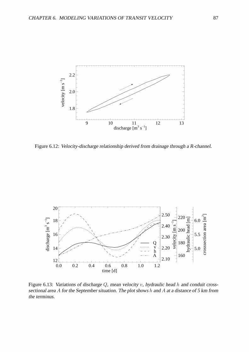
CHAPTER 6. MODELING VARIATIONS OF TRANSIT VELOCITY 87
9 10 11 12 13discharge [m3 s−1]
1.8
2.0
2.2
velo
city
[m s−
1 ]
Figure 6.12: Velocity-discharge relationship derived from drainage through a R-channel.
0.0 0.2 0.4 0.6 0.8 1.0 1.2time [d]
12
14
16
18
20
disc
harg
e [m
3 s−
1 ]
2.10
2.20
2.30
2.40
2.50
velo
city
[m s−
1 ]
160
180
200
220
hydr
aulic
hea
d [m
]
5.0
5.5
6.0
cros
ssec
tion
area
[m2 ]
QvhA
Figure 6.13: Variations of discharge Q, mean velocity v, hydraulic head h and conduit cross-sectional area A for the September situation. The plot shows h and A at a distance of 5 km fromthe terminus.

CHAPTER 6. MODELING VARIATIONS OF TRANSIT VELOCITY 88
12 14 16 18discharge [m3s−1]
2.2
2.4
velo
city
[m s−
1 ]
9 10 11 12 13discharge [m3 s−1]
1.8
2.0
2.2ve
loci
ty [m
s−1 ]
a b
Figure 6.14: Velocity-discharge relationships derived from scenarios representing the situationduring the August (a) and September (b) experiments.
In summary, the September scenario is dominated by an increase in discharge to which theconduit cross-sectional area A responds. In contrast, the pressure head h shows an inverseevolution and decreases as A increases although Q is rising. The resulting vQ-relationship(Fig. 6.14b) looks very different from the one obtained for the August scenario (Fig. 6.14a).This is attributed to the continuously rising discharge which does not show cyclic behavior.Due to the time lag of ∼6 h of A with respect to Q, the local maximum of A coincides withthe slight decline of Q. Consequently, h and therefore v are substantially reduced but rise assoon as discharge increases again. This is expressed in the pronounced V-shape of the vQ-plotin Figure 6.14b.
6.7.2 Retardation in a tributary moulin
Figure 6.15 illustrates the effects of inflow modulation at the junction of a tributary moulin to amain conduit. As shown before, variations of hydraulic head in a rigid pipe follow directly thoseof discharge (Sec. 6.7.1) and therefore, the hydraulic head hmoulin at the junction of moulin andconduit is proportional to Qconduit (Fig. 6.15a).
The supraglacial input into the moulin Qin precedes Qsub by 0.1 d but due to its small proportionof total discharge Qconduit, the influence of Qin on hydraulic conditions in the main channel isnegligible, thus Qconduit ≈ Qsub. However, with increasing size of the moulin cross-sectionalarea Amoulin, the transit velocity through the combined moulin-pipe system changes noticeablyin magnitude and timing (Fig. 6.15b). The reduction of transit velocity of an imaginary tracerdue to retardation in a moulin with Amoulin = 0.05 m2 is only weak, but Figure 6.16a demon-strates that the effect increases with size of the moulin Amoulin. At elevated values of hmoulin
the retardation of tracer is enhanced since the water column in the moulin through which thetracer travels becomes longer. Consequently, the relationship between hmoulin and transit ve-locity develops gradually into a anti-correlation (Fig. 6.16b) and velocity becomes increasinglycontrolled by the input discharge into the moulin. Furthermore, with an increase of the wa-ter volume in the moulin, the diurnal amplitude of transit velocity is significantly attenuated(Fig. 6.16c).
As before with the R-channel model (Sec. 6.7.1), the moulin-pipe model is used to simulate theplumbing of Unteraargletscher during the tracer experiments in August and September 2000.For this purpose, we use the same parameterization of the discharge situations as used above to

CHAPTER 6. MODELING VARIATIONS OF TRANSIT VELOCITY 89
0.0 0.2 0.4 0.6 0.8 1.0time [d]
1.0
1.5
2.0
2.5
3.0
velo
city
[m s−
1 ]
8.8
10.4
11.9
13.5
disc
harg
e [m
3 s−
1 ]
0.1
0.2
0.3
0.4
mou
lin in
put [
m3 s−
1 ]
100
150
200
hydr
aulic
hea
d [m
WC
]
Qsub
Qin
hmoulin
Amoulin [m2]
0.00 0.05
0.50
2.50
b
a
Figure 6.15: (a) Variation of prescribed discharge in the conduit Qsub (solid), the input intothe moulin Qin (dotted) and the hydraulic head hmoulin at the junction of moulin and conduit.(b) Comparison of velocity in the main conduit (solid) and transit velocity through the moulin-conduit system for several values of the moulin cross-sectional area Amoulin.

CHAPTER 6. MODELING VARIATIONS OF TRANSIT VELOCITY 90
0.0
−0.2
−0.4
−0.6
−0.8
−1.0
phas
e sh
ift [P
I]
0 2 4 6 8 10cross−sectional area of moulin [m2]
0.00
0.10
0.20
0.30
0.40
0.50
velo
city
am
plitu
de [m
s−1 ]
0.00
0.50
1.00
1.50
2.00
2.50
mea
n ve
loci
ty [m
s−1 ]
c
b
a
Figure 6.16: Effects of increasing inflow modulation in a tributary moulin on (a) transit velocity,(b) the phase shift between maximum velocity and peak discharge and (c) the diurnal amplitudeof transit velocity. The solid line connecting diamonds represents the value corresponding toa passage through the entire system and the asterisks connected by the dashed line refer to thevalue in the channel solely.

CHAPTER 6. MODELING VARIATIONS OF TRANSIT VELOCITY 91
12 14 16discharge [m3 s−1]
1.8
2.0
2.2
2.4
velo
city
[m s−
1 ]
9 10 11 12 13discharge [m3 s−1]
1.6
1.8
2.0
velo
city
[m s−
1 ]a b
Figure 6.17: Velocity-discharge relationships derived from scenarios representing inflow modu-lation in a moulin with Amoulin = 0.25 m2 during the August (a) and September (b) experiments.
derive Figure 6.14. Additionally, the input discharge into the moulin Qin is expressed as a sinefunction reproducing the measured supraglacial discharge (Fig. 5.2). Figure 6.17 illustratesthe velocity-discharge relationships obtained from the two scenarios. The size of the moulincross-section was selected such that the observed vQ-hysteresis is approximately reproduced.In both cases, Am = 0.25 m2 was used. The vQ-relationship of the August scenario displaysclockwise hysteresis while that of the September scenario is characterized by a pronounced V-shape. Similar to the results obtained with the R-channel model (Section above), the resultsobtained with the moulin-pipe model exhibit vQ-hystereses which resemble those observed bythe tracer experiments (Fig. 5.14).
6.8 Discussion
In this chapter we have derived a formulation to describe time dependent drainage througha subglacial channel. In a first application, we have investigated the general characteristicsof this model and compared them to those derived from an analytical steady-state solution(Röthlisberger, 1972). Further, we analyzed the variations of transit velocity in response todischarge variations similar to those observed in the field (Sec. 5.2.1). Here, our aim wasto simulate mechanisms which were supposed to account for the hystereses in observed vQ-relationships (Sec. 5.4.3). Considering the many assumptions which have to be made about aninaccessible environment, we prefer not to tune parameter values to obtain a good match ofmodel results and data. Hence, we focus on elucidating the behavior of a subglacial drainagesystem rather than on exactly reproducing values of limited reliability.
6.8.1 R-channel model
The results of our analysis of model behavior underline clearly the necessity for a time-dependent model of subglacial water flow. Especially for discharge variations with a periodof T = 1 d, a characteristic feature of glacial discharge, we observe substantial discrepanciesbetween the output of our time-dependent model and the steady-state solution of Röthlisberger(1972). Nevertheless, for discharge variations with long periods, predictions of the model ap-proach those calculated with the steady-state theory (Fig. 6.6). This contrasting behavior atdifferent time scales is caused by the time required for a conduit to adjust its size to changing

CHAPTER 6. MODELING VARIATIONS OF TRANSIT VELOCITY 92
hydraulic conditions. For long periods (T � 100 d), the evolution of the conduit cross-sectionoccurs fast enough such that a steady-state is reached, where opening and closure rates are bal-anced. In contrast, for short periods, the evolution of the conduit size cannot keep up pace withthe transient hydraulic conditions and a steady-state is not reached.
In response to the course of melt water production, glacial discharge displays a pronounceddiurnal variation which is superimposed to a longterm trend. As seen above, the drainage systemdoes not reach a steady-state at a time scale of one day and a time-dependent model is requiredto describe water flow through such a system appropriately.
Nevertheless, the use of the steady-state geometry as an initial condition for the conduit size canbe justified by the steep gradient of the curves in Figure 6.6 at short periods. This indicates thatmost of the system adjustment takes place within the first 10 days. Therefore, the assumptionthat a R-channel has adjusted to a mean discharge at intermediate time scales is acceptable.
6.8.2 Choice of roughness parameters
In Section 6.5.1, we have already stated that the values for f and k which were used to describethe roughness of subglacial conduits (Röthlisberger, 1972; Nye, 1976; Clarke, 1982; Spring andHutter, 1982; Hooke et al., 1990; Björnsson, 1998; Ng, 1998) are very high while at the sametime, by intuition one would expect an ice-walled conduit to be much smoother. Further, wehave also discussed that this discrepancy might be a result of our simplifying assumption of astraight conduit (Sec. 6.3.1). We visualize the flowpath as an irregularly meandering subglacialconduit. Since detailed information about the real course of such a conduit is not available, weconceptualize a simple model with one roughness parameter describing any kind of hydraulichead losses. Here, we would like to discuss to what extent physically plausible values for thefriction parameter of an ice-walled conduit are consistent with a value comprising local as wellas frictional losses.
With reference to Figure 6.18, we can express the total head loss ∆H by using a single losscoefficient ξ (e.g. Hager, 1995)
∆H = ξv2
2g, (6.30)
where ξ describes the combination of frictional losses in the ice-walled conduit fi and a numberd of local losses ξloc
ξ = fi∆x
4Rh
+ d ξloc. (6.31)
In our model formulation we lump these losses together into one effective friction factor f .Hence we can write
∆H = f∆x
4Rh
v2
2g. (6.32)
Equating this expression with Equation (6.30) and substituting Equation (6.31) yields d, thenumber of local losses required to explain the high value of f
d = (f − fi)∆x
4Rh
1
ξloc. (6.33)
By inserting typical values, we can calculate d and assess thereby how the value of our param-eter f might be composed. For now, we select fi = 0.01 (' k = 100 m1/3 s−1) and we will

CHAPTER 6. MODELING VARIATIONS OF TRANSIT VELOCITY 93
H
x
∆Hloc
∆H
∆x
∆x ’
Figure 6.18: The total hydraulic head loss ∆H over a distance ∆x expressed as a combinationof frictional losses along ∆x′ and local losses ∆Hloc (solid line). Alternatively, the dashed lineshows the same ∆H but expressed as a continuous head loss which is described by a single,effective loss coefficient.
discuss this choice below. Above, we visualized the conduit beneath Unteraargletscher as me-andering and being intersected by crevasses (Sec. 6.1). From the wide range of loss coefficientsfor bends, we choose ξloc = 1 for simplicity. This value corresponds to a sharp bend of theconduit. Further, we use ∆x = 5000 m, the length of our modeled conduit and Rh = 0.63 m.The latter value is the hydraulic radius of a circular conduit with a cross-sectional area of 5 m2.If we assign a value of 0.01 for fi and 0.5 for f , we obtain d = 972. One might also argue,that the roughness of a subglacial conduit is a composite of a smooth ice roof and a roughboulder-strewn bottom. If the sediments at the bottom comprise not more than 30% of theconduit perimeter and we assign fbottom=0.25 (' kbottom=20 m1/3 s−1) to the bottom part, thecombination yields a value fcom=0.02 (kcom=70 m1/3 s−1). In this case d = 952.
Further, we can try to assess the consequences for the choice of f related to the fact that the realcourse of the conduit is unknown. Below, we will discuss the discrepancy between measuredand modeled transit velocities. It appears that the modeled values systematically overestimatethe measurements by at least a factor of 3 (Sec. 6.8.3). Although we cannot attribute thisdifference directly to differences in path length, it is obvious, that the real flowpath must belonger than the straight-line distance as assumed in the model. Hence, as a rough estimate weassume that the real length of the conduit is double its straight-line length. Then, we insert∆xreal=2 ∆x into Equation (6.31) while Equation (6.32) remains unchanged. Then
d = (f − 2 fi)∆x
4Rh
1
ξloc.
and the resulting values of d are 952 and 912 for the 0.01 and 0.02 estimates for fi and fcom,respectively.
Although we have considered different situations, enveloped by a smooth, ice-walled conduithaving a circular cross-section and following a straight line on the one hand and a meanderingconduit at the bed having a composite roughness on the other hand, the number of local losses

CHAPTER 6. MODELING VARIATIONS OF TRANSIT VELOCITY 94
required to explain the high value of a lumped losses parameter (f = 0.5), is in a narrow rangefrom 972 to 912. Along a straight-line length of 5000 m, this corresponds to one local loss aboutevery 5 m, a value which appears to be plausible for a meandering conduit.
Further, we discuss our selection of fi and the formerly introduced assumption of f beingconstant. An ice-walled conduit might be appropriately described as hydraulically smooth.In this case, the Colebrook-White equation (e.g. Hager, 1995) simplifies to
f−1/2 = −2 lg(
2.51
Re f 1/2
)
, (6.34)
where Re = 4vRh/ν is the Reynolds-number with ν = 1.79× 10⁻⁶ m2 s−1 being the kinematicviscosity of water. In the different scenarios which were considered by our model, Reynolds-numbers range from 4.3 × 10⁵ to 3.7 × 10⁶. Using Equation (6.34) yields values for fi varyingbetween 0.009 and 0.013. Hence, fi = 0.01 is an appropriate choice for our purpose to assessthe composition of our effective loss parameter f .
While local losses are independent of Reynolds-numbers, frictional losses vary with Re. Al-though this dependence attenuates for high values of Re, we have seen that in our scenariosfi varies with Re. Hence, the assumption of a single, constant value introduces an error of±20%. However, using our considerations above, we can determine the portion of the totalhead loss which occurs locally (dξloc)/ξ. For the range of values determined for d, we find thatlocal losses contribute 92-98% to the total loss. With maximal 8% of the loss depending on theReynolds-number, the maximum inaccuracy due to the assumption of a constant f amounts to8% ×±20% = ±1.6% and is therefore negligible.
6.8.3 Velocity variations due to a dynamic geometry
If we compare the results of our calculations to the measurements, it appears that the magni-tudes of modeled velocity exceed systematically the values derived from the tracer experiments.This shortcoming is mainly associated with the fact that the real length of the flow path in natureis unknown and the straight-line assumption for the calculation of velocity represents a mini-mum estimate. Consequently, any modeled transit velocity overestimates the measured data.Further possible sources of discrepancy are attributed to the assumption of a circular conduitcross-section and the choice of roughness (Equations (6.9) and (6.11)) and flow law parameters(Equation (6.6)).
Table 6.3 summarizes the results of a sensitivity study which was carried out to illuminate theeffects of parameter uncertainties on the model results in terms of water pressure and transitvelocity. The roughness parameters k and f were varied in a range which appears plausiblefor the roughness of a proglacial stream (Röthlisberger, 1972). The flow law coefficient B waschanged to values representing each a slightly softer and a slightly stiffer ice. For the caseof softer ice, we adopted a value determined by Gudmundsson (1994, 1999) from comparingmeasured and modeled surface velocities in the confluence area of Unteraargletscher. The valueof B used by Bauder (2001) in his flow model of entire Unteraargletscher is also smaller thanthe one used by us. However, we have to bear in mind, that both authors have neglected basalmotion in their model formulation and therefore they had to overestimate ice-deformation toachieve agreement between measured and modeled surface velocities. Therefore, we regardthis value as a minimum estimate for our parameter B. We prefer to use a value determined

CHAPTER 6. MODELING VARIATIONS OF TRANSIT VELOCITY 95
Table 6.3: Sensitivity of model results to uncertainties in conduit roughness k [ m1/3 s−1], f [-]and flow law coefficient B [ Pa−3s−1].
Pressure head VelocityDescription Parameter valuerange [m] range [ m s−1]
k = 15 f = 0.5referenceB = 5.3 × 10⁻²⁴ 85–203 1.7–2.2
enhanced roughness k = 10 f = 1.1 97–233 1.3–1.6reduced roughness k = 20 f = 0.3 76–189 2.1–2.6softer ice B = 6.8 × 10⁻²⁴ 104–244 1.8–2.3stiffer ice B = 2.4 × 10⁻²⁴ 65–168 1.6–2.1
by Nye (1953) using measured closure-rates of glacier tunnels. The value for stiffer ice wasadopted from Paterson (1994).
It turns out that an enhanced conduit roughness increases the resistance of the conduit andtherefore, the hydraulic gradient required to drive the flow increases but the transit velocity isreduced. Further, a softer ice would permit enhanced closure rates. Hence, a smaller conduitwould require an enhanced hydraulic head to drive the flow thereby increasing the velocity.Thus, changes in channel roughness and ice-stiffness which affect the water pressure in a similarway have contrary effects on transit velocity. This finding demonstrates that without furtherconstraints on parameter values, fitting the model to measured data would not provide a gain ofinformation.
In conclusion, the modeling work supports the hypothesis that the dynamic geometry of a R-channel could account for hysteresis in the vQ-relationships derived from tracer experiments(Chapter 5). In contrast, such hysteretic behavior cannot be explained by routing an identicaldischarge through a static pipe.
6.8.4 Velocity variations due to inflow modulation
In analogy to the discussion of consequences of a dynamic conduit geometry, we now considerthe results of the moulin model with respect to variations of transit velocity (Fig. 6.17). Weshould recall here, that in this model we described the conduit as a rigid pipe. Since this pipe hasthe same steady-state geometry as used in the preceding scenarios and the model was applied toan identical discharge variation, the velocities in the conduit itself are similar to those obtainedfrom the pipe model (Fig. 6.9). Additional variations of transit velocity through the entiresystem are caused by retardation of the water flow in a moulin. Consequently, the magnitudeof transit velocity is reduced. The retardation depends directly on the volume of the moulin,expressed by the parameter Amoulin which is unknown. The idea of a moulin being a verticalslot of uniform cross-section is certainly a strong oversimplification of the natural phenomenon.However, the equations for an inclined moulin look identical to those of a vertical one if aneffective cross-section Aeff = Ainc/ cosΦ is used instead of Amoulin. Here, the angle Φ denotesthe deviation from vertical and Ainc is the cross-sectional area of the inclined moulin. Thus,Amoulin can be understood as an effective cross-sectional area averaged over the depth of themoulin.

CHAPTER 6. MODELING VARIATIONS OF TRANSIT VELOCITY 96
Figure 6.16b shows clearly that a phase shift between transit velocity through a moulin-conduitsystem and main discharge can be produced by retardation of water in a moulin. Further, theeffect depends on the magnitude of Amoulin. In consequence, the model enables any phase shiftbetween 0 and −π independent of the considered period of discharge variation. In contrast, thephase shift between discharge and velocity in a dynamic conduit is strongly dependent of theperiod. Finally, we conclude that inflow modulation at the junction of a tributary moulin to amain conduit is a valid mechanism to explain vQ-hysteresis.

Chapter 7
Modeling variations of tracer dispersion
In Chapter 6 we have validated the hypotheses that the dynamic geometry of a R-channel aswell as hydraulic damming at the junction of a moulin and a conduit can both account for hys-teresis in the vQ-relationship. Based on the interdependence of discharge, conduit size andtransit velocity in a Röthlisberger-channel, we suggested a positive relationship between con-duit size and dispersion coefficient to explain the observed hysteresis in the velocity-dispersionrelationship (Sec. 5.4.3). Alternatively, for the case of transit velocities being controlled byhydraulic damming, we postulated that increasing retardation in a moulin causes higher disper-sion coefficients (Sec. 5.4.3). However, the model which was used in Chapter 6 considers onlythe variations in transit velocity but does not account for tracer dispersion. Thus, we have todevelop an independent approach to test whether the variations of tracer dispersion are consis-tent with the interpretations drawn from the velocity variations. For this purpose, numericaltracer tests were performed to study systematically the influence of geometry changes on tracerdispersion. Therefore, a model is adopted which was used by Hauns (1999) and Hauns et al.(1998) to investigate the retardation of water flow in karst conduits of different geometries. Nu-merical tracer experiments are performed by propagating a scalar field representing the tracerwith the velocity field through a simplified flow geometry. Hauns et al. (1998) have validatedthe model with accompanying laboratory experiments. In this study, we adapt this model toseveral idealized conduits which differ in size, shape or roughness. With each conduit scenario,tracer return curves were generated for different hydraulic conditions.
7.1 Turbulent flow field
The Navier-Stokes equations describe laminar flow of an incompressible and isothermal fluid.The set of governing equations comprises an expression for conservation of mass:
∇ · v = 0 (7.1)
and one for conservation of momentum:
∂
∂tρv + ∇ · (ρv ⊗ v) = −∇p + ∆(µv) + B. (7.2)
Here v is the fluid velocity, ρ denotes the fluid density, p and t are pressure and time, respec-tively. Further, B is a body force and µ is molecular viscosity.
97

CHAPTER 7. MODELING VARIATIONS OF TRACER DISPERSION 98
However, flow through subglacial conduits is considered to be turbulent (Röthlisberger, 1972;Weertman, 1972). Nevertheless, the Navier-Stokes equations are valid for turbulent flow as wellsince turbulent flow can be considered also as a very complex unsteady laminar flow. However,it is not feasible to solve the Navier-Stokes equations accurately for high Reynolds-numbers.Therefore, we have to resort to turbulence modeling. The fundamental procedure in turbulencemodeling is to split the field quantities each into a mean and a fluctuating part:
Φ = Φ + Φ′
Ψ = Ψ + Ψ′,(7.3)
where Φ and Ψ denote two arbitrary field quantities. Equation 7.3 is subject to the followingconditions:
1. Φ = Φ and Φ′ = 0
2. ΦΨ = ΦΨ
3. ΦΨ′ = 0
4. ΦΨ = ΦΨ + Φ′Ψ′.
Applying this method to the Navier-Stokes equations, the continuity equation becomes:
∇ · v = 0 (7.4)
and the momentum equation is written:
∂
∂tρv + ∇ · (ρv ⊗ v) = −∇p + ∆(µv) −∇ · (ρv′ ⊗ v′), (7.5)
where the body force was dropped for clarity. The additional turbulent flux term ∇ · (ρv ′ ⊗ v′)has the dimension of a stress and is also known as Reynolds-stress. This term cannot be calcu-lated explicitly and is therefore parameterized by the k-ε-approach which introduces a turbulentviscosity µT = cµρk2
εto describe the Reynolds-stress
∇ · (ρv′ ⊗ v′) = µT (∇v + ∇vT ). (7.6)
Here, k is the turbulent kinetic energy and ε represents the turbulence dissipation rate, cµ is aconstant. Empirical expressions or values for k, ε and cµ were adopted from CFX (1996).
7.2 Model description
The approach consists in describing the three-dimensional velocity field of turbulent dischargethrough a given geometry. Subsequently, tracer transit is simulated by a scalar volume whichis propagated through this flow field by advection and diffusion. For the numerical tracer ex-periments, we used the commercial package CFX-4.3 of AEA Technology which provides acomplete environment to solve turbulent flow problems.

CHAPTER 7. MODELING VARIATIONS OF TRACER DISPERSION 99
0.5 m
10 mx
z
y
AH
Figure 7.1: The idealized conduit geometry through which numerical tracer tests were per-formed. Water flow is in x-direction.
7.2.1 Numerics
The set of equations for the turbulent velocity-field was discretized using a finite volumes andsolved using finite differences. Therefore, the flow geometry was subdivided into a grid ofrectangular volumes using the CFX mesh-generator. Each equation was integrated over eachcontrol volume to obtain a discrete equation which connects the variable at the center of thecontrol volume to its neighbors. All terms were discretized in space using a hybrid differencingscheme, whereby upwind differencing was used for advection terms where advection dominatesdiffusion and central differencing otherwise. In an upwind scheme, the value of the variable istaken from the upstream neighbor, whereas in central differencing the mean value between twoneighbors is assigned to the variable. These procedures are used as the default by CFX-4.3 CFX(1996).
7.2.2 Model geometry
The procedure was applied to an idealized conduit which was represented by a rectangulargeometry (Fig. 7.1). Numerical integration of the model equations requires boundary conditionsat the margins of the geometry. Where the water flow is constrained by a solid boundary, ano-slip condition for velocity was applied. The amount and direction of water discharge isdefined by adequate boundary conditions at the inlet and outlet cross-section. Inflow of waterwas represented by a constant two-dimensional velocity field pointing into the model regionwhereas a no-pressure condition was prescribed at the outlet plane. Since the considered modelgeometries here are horizontal, the water flow is driven only by the pressure gradient which isrequired to match the mass flow condition at the inlet.
7.2.3 Tracer transport
In the stationary velocity field which is then obtained, transport of a conservative tracer is simu-lated by an advective-diffusive propagation of a scalar Θ representing the tracer concentration:
∂
∂tΘ = −∇ · (v Θ + Dm∇Θ), (7.7)
where Dm represents the coefficient of molecular diffusion. Although the diffusion process isirrelevant for the tracer transport since hydrodynamic dispersion is several orders of magnitudelarger, a non-zero value for Dm is required by the solver to obtain a stable solution (CFX,

CHAPTER 7. MODELING VARIATIONS OF TRACER DISPERSION 100
>0.420.350.280.210.140.070.00
5 s
10 s
15 s
20 s
25 s
x
y
1 s
Figure 7.2: Illustration of simulated tracer distribution in the xy-plane at half height of theconduit at different time steps after injection. Flow is in x-direction and the color bar denotesthe tracer concentration relative to its input value.

CHAPTER 7. MODELING VARIATIONS OF TRACER DISPERSION 101
I OF
Figure 7.3: A black-box procedure F transforms an input I to a system output O.
1996). Therefore, a very small value of 10−13 m2 s−1 was used. As such, the approach is validonly if the tracer’s influence on the fluid density is negligible. This is typically the case inthe experiments at Unteraargletscher where maximum observed dye tracer concentrations werelower than 20 ppm. Tracer breakthrough curves were obtained by recording the scalar fluxthrough the outlet plane.
Figure 7.2 shows an example of how the tracer cloud propagates through the conduit. Duringtransit, the initially compact field becomes increasingly dispersed concurrent with a decrease ofmaximum concentration. Further, there is a backwards bending of the concentration contoursnoticeable. It increases with travel time and reflects the retarding influence of the conduit walls.
7.2.4 Extending the length scale
The explicit modeling of turbulent flow and tracer transport is restricted to length scales on theorder of 100 − 101 m since for longer dimensions the computational effort becomes excessive.However, natural tracer tests are typically performed over length scales of 102 − 103 m. Thishas to be taken into account since roughness elements can cause significant tracer retardationat the meter scale. However, at the 102 − 103 m scale roughness might rather contribute todispersion as the retardation effect is repeated regularly (Hauns et al., 2001). Therefore, anadditional approach is required to investigate the behavior of the considered conduits at a scalerepresentative of our field situation. Here, a simple black box model is applied. This approachentails that once the transfer function of a simulated conduit segment is determined, scenariosfor conduits of any desired length can be generated by multiple concatenation of such transferfunctions (Box et al., 1994).
Convolution
The transfer-function F is a convolution operator which describes the transformation of an inputsignal I into a system output O, even though the exact physical process of that transformationremains unknown or is ignored (Fig. 7.3). In the problem considered here, the tracer is conser-vative, therefore the system can be considered as a single-degree-of-freedom system with thetemporal distribution of concentration ∂
∂tΘ as the only degree of freedom. Then, the convolution
can be performed in the time domain by Duhamel’s Integral (expressed in discretized form):
Om =m∑
n=0
FnIm−n. (7.8)
Here, the subscript m denotes the considered time step and n represents the time steps between0 and m.
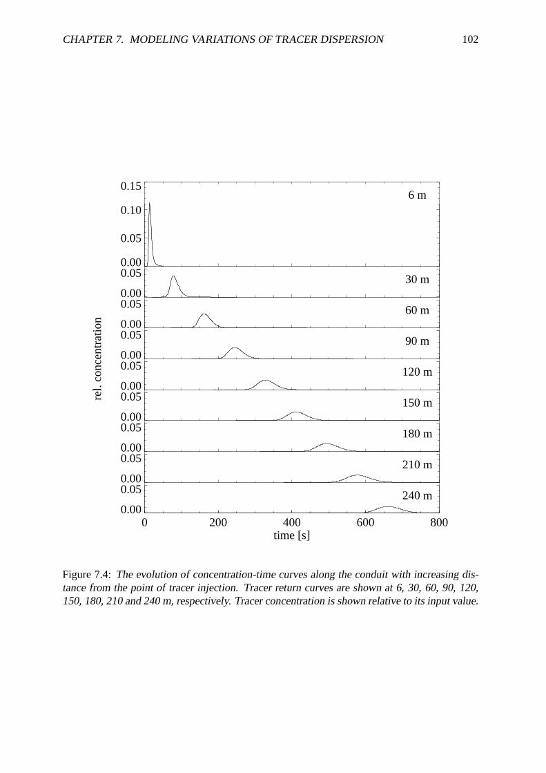
CHAPTER 7. MODELING VARIATIONS OF TRACER DISPERSION 102
0.00
0.05
0.10
0.15 6 m
0.00
0.05 30 m
0.00
0.05 60 m
0.00
0.05 90 m
0.00
0.05 120 m
0.00
0.05 150 m
0.00
0.05 180 m
0.00
0.05 210 m
0.00
0.05 240 m
0 200 400 600 800time [s]
rel.
conc
entr
atio
n
Figure 7.4: The evolution of concentration-time curves along the conduit with increasing dis-tance from the point of tracer injection. Tracer return curves are shown at 6, 30, 60, 90, 120,150, 180, 210 and 240 m, respectively. Tracer concentration is shown relative to its input value.

CHAPTER 7. MODELING VARIATIONS OF TRACER DISPERSION 103
0 50 100 150 200 250distance from injection point [m]
0.050
0.060
0.070
0.080
0.090
0.100
disp
ersi
on c
oeffi
cien
t [m2 s
−1 ]
5
10
15
reta
rdat
ion
[%]
Figure 7.5: The evolution of dispersion coefficient (solid) and retardation (dashed) of the tracerbreakthrough curves shown in Figure 7.4 with increasing distance from the injection site. Re-tardation is quantified by the portion of the tracer mass, which is not accounted for by theadvection-dispersion model (cf. Sec. 5.2.3).
Deconvolution
With the knowledge of the system output function O in response to a known input signal I , thetransfer function F can be obtained by deconvolution:
Fm =1
I0
(Om −
m∑
n=1
(Fm−nIn)). (7.9)
Although, this is an efficient method to determine the transfer function, it suffers in many casesfrom numerical instability (Box et al., 1994). However, in this application, the input functionconsists of a simple, rectangular pulse and the procedure proofed to be non-problematic. OnceF is obtained, its convolution with any input function is very robust.
7.2.5 Model performance
Once the hydraulic solution was found, transport of tracer through the stationary flow fieldwas simulated. To initiate the tracer transport, the scalar-field used to represent the tracer wasset equal to 1 at the inlet cross-section during 2 seconds. The scalar-tracer field was recordedat the outlet cross-section and its time series is analogue to a tracer return curve. From thisreturn curve, we constructed the corresponding transfer-function by deconvolution and usedthis subsequently to derive return curves for a 240 m long flow path.
Figure 7.4 illustrates how the shape of a return curve evolves with increasing length of theconduit. Tracer concentration was logged at several sections along the flow path. The firstbreakthrough curve displays an asymmetrical shape which is characterized by a steep rise anda long-lasting decline, indicative of pronounced retardation. With increasing length of the con-duit, the asymmetry of the return curve decreases gradually, peak concentrations decline andcurves become broader. This evolution was quantified by using the advection-dispersion modelas described in Chapter 4 and Section 5.2.3. Figure 7.5 shows how the dispersion coefficient

CHAPTER 7. MODELING VARIATIONS OF TRACER DISPERSION 104
Table 7.1: Different tracer tests performed to study the effect of conduit size on tracer disper-sion. Discharge Q was routed through the conduit of cross-sectional area A with a mean flowvelocity v0.
no. Q [l/s] v0 [m/s] A [m2]
c1 10. 0.173 0.0576c2 15. 0.261 0.0576c3 20. 0.347 0.0576c4 34.6 0.600 0.0576c5 15. 0.221 0.0677c6 20. 0.295 0.0677c7 23.5 0.347 0.0677c8 40.6 0.600 0.0677c9 25. 0.200 0.125c10 43.4 0.347 0.125c11 75. 0.600 0.125
Table 7.2: Different tracer tests performed to study the effects of conduit shape on tracer dis-persion.
no. H [m] W [m] Rh [m]
r1 0.5 0.5 0.125r2 0.25 1.0 0.100r3 0.125 2.0 0.058r4 0.0625 4.0 0.031
increases with the length of the flow path concurrent with a decrease of retardation. This obser-vation demonstrates how tracer retardation at short spatial scales contributes to hydrodynamicdispersion at larger spatial scales.
7.3 Experiments
To study systematically the influence on tracer dispersion in different scenarios, the conduitgeometry was altered in size, width to height ratio and roughness. To characterize the dispersivebehavior of each of these scenarios, we derived velocity-dispersion relationships by using anumber of different flow velocities.
In a first experiment, the height H of the conduit geometry was varied to generate conduits withdifferent cross-sectional areas A. Table 7.1 lists details of individual experiments.
Another set of tracer tests was designed to study the influence of the cross-sectional shape.Since the flow velocity is zero at the conduit walls, the flow field and therefore also the tracertransport is affected by the fraction of water that is in contact with the wall. This influencecan be examined by systematically varying the hydraulic radius Rh = A/U , where A is thecross-sectional area that is occupied by the water and U is the wetted perimeter of the conduit.The mean flow velocity v0 = 0.3 m s−1 was kept constant in the four cases performed. Detailsare presented in Table 7.2.

CHAPTER 7. MODELING VARIATIONS OF TRACER DISPERSION 105
y
za
b
c
Figure 7.6: Cross-sectional profiles of the three conduits which were used to study the effect ofroughness on tracer dispersion. Water flow is into the page.
0.420.350.280.210.140.070.00x
y1 m
Figure 7.7: Tracer distribution in the xy-plane at 0.04 m height of the conduit shown in Fig-ure 7.6c. The situation represents a snapshot at 20 s after introduction of the tracer. Water flowis in x-direction. The color bar denotes tracer concentration relative to its input value. Locationof the obstacles is indicated by the white squares.

CHAPTER 7. MODELING VARIATIONS OF TRACER DISPERSION 106
0.20 0.30 0.40 0.50 0.60 0.70transit velocity [m s−1]
0.02
0.04
0.06
0.08
0.10
disp
ersi
on c
oeffi
cien
t [m2 s
−1 ]
Figure 7.8: Velocity-dispersion relationships for three conduits of different cross-sectional area.Solid circles connected with a dashed line denote the small conduit, open diamonds on a solidline mark the medium size and solid triangles again connected with dashes represent the largeconduit.
A third set of return curves was generated to investigate the effect of changes in roughness ontracer dispersion. A mean flow velocity v0 = 0.3 m s−1 was kept constant throughout theseexperiments. Roughness was introduced into the conduit by distributing rectangular obstaclesat the bottom of the conduit (Fig. 7.6). The obstacles are 0.2×0.2×0.1 m in size and are meantto represent roughness elements typical for a glacial stream. Roughness enhances turbulence inthe flow-field thereby affecting the transport of a tracer. Figure 7.7 illustrates how the tracer isretarded in the flow-reversals at the lee side of the obstacles.
Before introducing obstacles, a reference experiment was conducted (Scenario ’a’ in Fig. 7.6).A second test consisted of the same configuration but containing obstacles (Fig. 7.6b). In a thirdscenario, the influence of the bottom roughness was increased. This was achieved by broadeningthe conduit and to conserve the cross-sectional area, the ceiling was shaped asymmetrically(Fig. 7.6c).
7.4 Results
Results of the 11 experiments performed to study the interdependence of tracer dispersion andcross-sectional area are presented in Figure 7.8. Velocity-dispersion relationships are shownfor each of the three different conduit sizes. The curves feature a positive relationship betweentransit velocity and the dispersion coefficient with the slope of the curves increasing towardshigher velocity. The dependence of dispersion coefficients on cross-sectional area is expressedby different curves described for differently sized conduits. It reveals that a larger conduit yieldssystematically higher dispersion coefficients than a smaller one.
Results from varying the hydraulic radius at constant flow velocity and constant cross-sectionalarea are shown in Figure 7.9. We can perform an extrapolation of the graph with two additional

CHAPTER 7. MODELING VARIATIONS OF TRACER DISPERSION 107
0.00 0.05 0.10 0.15hydraulic radius [m]
0.00
0.02di
sper
sion
coe
ffici
ent [
m2 s−
1 ]
v0 = 0.3 [m s−1]
Figure 7.9: Effect of the hydraulic radius on dispersion. The flow velocity was kept constantin all scenarios. The dashed lines denote extrapolations of the relationship based on data fromHauns et al. (2001). See text for details.
Table 7.3: Dispersion coefficients obtained from varying the influence of roughness in the con-duit geometry.
scenario Rh [m] D [m2 s−1] remarks
a 0.0706 0.01717 no additional roughnessb 0.0706 0.05906 additional roughnessc 0.0614 0.09783 enhanced influence of roughness
points. First, we consider the trivial case D = 0 for Rh = 0 and second, we adopt a valuedetermined by Hauns et al. (2001) for a perfectly homogeneous velocity field. This conditionis realized for an infinitely high and wide conduit. Therefore Rh → ∞ and it was foundD∞ = 0.045 m2 s−1 for v = 0.3 m s−1. The figure demonstrates that with increasing hydraulicradius, dispersion approaches asymptotically D∞.
Table 7.3 lists results of the three experiments performed to investigate the effect of roughnesson tracer dispersion. Comparison of Scenarios ’a’ and ’b’ shows that introduction of obstaclesinto the conduit causes a substantial increase of the dispersion coefficient. If the influence ofroughness is further increased as considered in Scenario ’c’, the dispersion coefficient increaseseven more, although the hydraulic radius of this conduit is reduced with respect to that ofScenario ’a’ or ’b’.
7.5 Discussion
In this chapter, we performed numerical tracer tests to study systematically the effect of changesof the conduit geometry on tracer dispersion. The results of our experiments indicate a positiverelationship between the dispersion coefficient D and cross-sectional area of the conduit A.

CHAPTER 7. MODELING VARIATIONS OF TRACER DISPERSION 108
Such a relationship was postulated in Chapter 5 where variations of tracer dispersion werediscussed in relation to variations of transit velocity.
However, the dependence of D on A as illustrated in Figure 7.8 is not very strong. In these ex-amples the increase in size was accomplished by heightening a rectangular conduit of constantwidth. This involves a change of the perimeter and thereby the influence of the conduit-wall isaltered. Here, the influence of the conduit-wall was expressed in terms of hydraulic radius Rh.Figure 7.9 reveals that an increase of hydraulic radius at constant cross-sectional area also in-creases the dispersion coefficient. However, this effect is relevant only for hydraulic radii belowthe meter scale. Towards larger values of Rh, the increase of D is attenuated and the dispersioncoefficient approaches a maximum value. This indicates that the increase of dispersion coeffi-cients in Figure 7.8 would also approach an upper limit since an increase of the cross-sectionalarea is accompanied by an increase of Rh. Results of simulating the conduit evolution in Chap-ter 6 suggest a cross-sectional area of the subglacial channel beneath Unteraargletscher on theorder of 100 m2. On this scale, the effect on tracer dispersion from changes in conduit size alonewould be very weak.
In contrast, a positive relationship between A and D was reported by Taylor (1954), but hisexperiments were conducted using pipes of a few centimeters in diameter. As discussed above,the increase of D attenuates towards larger values of Rh.
Further, it is shown by our experiments that the dispersion coefficient is strongly affected bychanges in roughness (Table 7.3) such that increased roughness generates enhanced dispersion.If conduit-increase entails a roughness increase, the tracer dispersion would be enhanced atthe same time. And if further roughness recedes after the termination of conduit-increase, thedispersion coefficient would decrease to a lower level. This argumentation provides a possibilityto interpret the observed velocity-dispersion hystereses using the R-channel model.
For our numerical tracer tests, we assumed a constant size and roughness along a straight,rectangular conduit which is certainly a strong simplification of the investigated flow path onUnteraargletscher. Instead, the conduit in nature might be curved with size and roughnesschanging along its length thereby causing significantly higher dispersion coefficients than thoseobtained from our idealized experiments. A roughness change as required by our interpretationmight be accomplished by either a nonuniform conduit growth or by erosion and sedimentationof subglacial sediments at the bottom of the conduit.
If hydraulic damming occurs, the effects on tracer dispersion are well comprehensible. We re-call that water flow occurs at a lower speed in the moulin and at a higher one in the conduit andthat the measured transit velocity represents an average value over the entire system. Let us con-sider two identical transit velocities, one is obtained from a drainage system where water flowshomogeneously with a constant velocity and the other one is affected by hydraulic damming,such that the retardation in the moulin must be compensated by a higher flow velocity in theconduit. Figure 7.8 demonstrates that higher flow velocities coincide with enhanced dispersion.Therefore, the case which is more affected by hydraulic damming would yield a higher dis-persion coefficient due to a higher flow velocity in the conduit. This conclusion confirms thepositive relationship between tracer dispersion and retardation in a moulin which was suggestedin Chapter 5 from field experiments.
Finally, as already indicated by the analysis of velocity variations (Chap. 6), we can concludethat a dynamic conduit geometry and hydraulic damming in a moulin are both equally validmechanisms to explain the observed behavior of tracer dispersion.

Chapter 8
Synthesis
8.1 Concluding discussion
In this thesis, the drainage of water through and from Unteraargletscher was studied with par-ticular emphasis on the internal plumbing and its behavior with time. Valuable insight into anotherwise inaccessible system was obtained by tracer experiments which were designed appro-priately to take particularities of a subglacial drainage system into account.
Tracer injections into a moulin of Unteraargletscher were repeated in quick succession overa number of diurnal discharge cycles to characterize the instantaneous state of the drainagesystem. Results are within the range found in previous comparable studies (Collins, 1982;Burkimsher, 1983; Nienow et al., 1996c). It is generally accepted to associate high veloci-ties in combination with low dispersion coefficients with a hydraulically efficient, channelizeddrainage system (e.g. Behrens et al., 1975; Lang et al., 1979; Collins, 1982; Burkimsher, 1983;Seaberg et al., 1988; Hock and Hooke, 1993; Fountain, 1993; Nienow et al., 1996b; Nienow etal., 1998; Wagnon et al., 1998; Hock et al., 1999; Hasnain et al., 2001). On the other hand, tran-sit velocities lower than 0.2 m s−1 were occasionally interpreted as typical for a less efficient,distributed drainage system (Hubbard and Nienow, 1997; Hasnain et al., 2001). However, ourresults exhibit a pronounced diurnal variation of transit velocity and tracer dispersion with min-imum values of transit velocity below this limit. Since all tests were performed in the sameflow path, there is little doubt that these variations reflect changing hydraulic conditions in thisparticular channel rather than morphological switching between distributed and channelizeddrainage configurations.
This finding underlines the major difficulty to detect a possible evolution of the drainage systembased on single tracer tests conducted at coarse temporal intervals. Single tests represent onlyrandom situations within a pronounced diurnal range. Therefore, different transport parametersderived from single tracer injections can be caused both by different hydraulic conditions andby different morphologies of the drainage system. Hence, to deduce extensive morphologicalchanges in the drainage system based on single tracer tests (e.g. Hasnain et al., 2001) is oflimited value. Instead, the inference of a drainage system evolution is much better defined if therange of transit velocities over a diurnal discharge cycle is taken into account and therefore, theobtained interpretation is more reliable.
Observed values of the dispersion coefficient are within the wide range described in previousstudies of subglacial drainage systems (e.g. Behrens et al., 1975; Seaberg et al., 1988; Willis et
109

CHAPTER 8. SYNTHESIS 110
al., 1990; Hock and Hooke, 1993; Hubbard and Nienow, 1997; Nienow et al., 1998). Only a fewauthors show the quality of their parameter estimation and discuss the reliability of the appliedtransport model (Seaberg et al., 1988; Willis et al., 1990; Hock and Hooke, 1993; Fountain,1993). However, a reliable estimate of transport parameters requires a careful inversion of theobtained tracer return curve by an adequate transport model. In this study, it is shown thatreliable parameter values can be obtained by fitting a simple advection-dispersion model to therising limb of an asymmetric tracer return curve. As such, only the part of the data which isadequately described by the model is evaluated. This approach was validated by comparisonwith the mobile-immobile model which accounts for storage-retardation processes.
Our experiments reveal a pronounced, clockwise velocity-discharge hysteresis thereby inhibit-ing the application of known methods to infer hydraulic conditions of the flow path. All ofthe previously established methods (Fountain, 1993; Kohler, 1995; Seaberg et al., 1988; Hockand Hooke, 1993) are based on the assumption that there exists a unique functional relationshipbetween velocity and discharge. Hysteretic behavior was observed by Nienow et al. (1996b)who reports also the occurrence of counterclockwise vQ-hysteresis. Such behavior has beeninterpreted to result from a two-component drainage configuration where discharge in the trib-utary conduit varies out of phase with that in the main conduit (Collins, 1995; Nienow et al.,1996b). However, the only attempt to date to simulate velocity-discharge hysteresis (Nienowet al., 1996b) is described by purely empirical relations and suffers from equifinality.
In this thesis, two mechanisms were identified which can account for hystereses in the velocity-discharge relationships. Such complex velocity-discharge relationships can be produced by adynamic conduit geometry as proposed for a Röthlisberger-channel or by hydraulic dammingat the junction of a two conduits carrying different discharges. With a physically based modelof subglacial water flow, each hypothesis was tested. The results suggest that both mechanismsprovide equally valid explanations.
The analysis of diurnal variations of the dispersion coefficient were used as an additional ap-proach to validate the explanation derived from variations of transit velocity. Similarly, a pro-nounced hysteresis in the velocity-dispersion relationship renders conventional interpretationtechniques inapplicable. Usually, a linear relationship between dispersion and velocity is as-sumed (e.g. Behrens et al., 1975; Brugman, 1986; Seaberg et al., 1988; Willis et al., 1990;Nienow et al., 1998) and the factor of proportionality, named “dispersivity” is calculated whichshould provide an independent measure of the dispersive behavior of the considered system.However, this interpretation is valid only in the case of a strictly linear velocity-dispersion re-lationship (Kinzelbach, 1992). This condition is obviously not fulfilled by the dataset whichwas obtained in this study. Instead, the influence of changes in conduit size or roughness ontracer dispersion was investigated using a numerical model of tracer transport through an ideal-ized geometry. Results suggest that a dynamical conduit geometry can account for the observedvelocity-dispersion relationship, especially, if the evolution of the conduit involves also changesin its roughness. Further, the effect of hydraulic damming on tracer dispersion is found to pro-vide an equivalent explanation for the observed behavior.
In conclusion, hysteresis in velocity-discharge and in velocity-dispersion relationships can beequally caused by a dynamic conduit geometry or by hydraulic damming in a tributary. Sinceeither of the mechanisms is highly plausible and neither of them can be excluded, a combinationof both is probably the most realistic configuration in nature.
This conception of multicomponent water transfer through the interior of a glacier has importantimplications for the interpretation of tracer experiments conducted in glacial drainage systems.

CHAPTER 8. SYNTHESIS 111
The transit time of water entering a moulin is affected by englacial storage as well as subglacialrouting processes and therefore both mechanisms have to be considered when hydraulic param-eters are to be inferred from tracer tests. Especially, if tracer tests are performed to investigatesubglacial drainage conditions, the influence of hydraulic damming on tracer transit has to betaken into account.
Our analysis of the water balance at Unteraargletscher provides evidence for englacial or sub-glacial storage which is related to the structure of the drainage system. Comparison of meltwa-ter input and proglacial discharge revealed that a significant amount of water was temporarilystored in or beneath the glacier which was subsequently released during a reconfiguration of thesubglacial drainage system.
8.2 Outlook
Tracer experiments represent undoubtedly a valuable approach to infer characteristics of sub-glacial drainage systems. However, in this study it is demonstrated that the inference ofhydraulic conditions at the glacier bed is complicated if the tracer passes through a multi-component system. The reliability of such an inference will be significantly increased if asubglacial channel could be investigated in isolation. This can be achieved by an injection oftracer directly into the channel, for instance through a borehole. The problem of locating asubglacial conduit was tackled by Sharp et al. (1993) who mapped the hydraulic potential ofHaut Glacier d’Arolla.. Based on these results, a dense set of boreholes has been drilled acrossthe region where a preferential drainage axis was predicted (Hubbard et al., 1995).
Furthermore, informations on the moulin geometry or measurements of the water level in themoulin concurrent with the tracer tests will help to constrain the representation of the moulinin a two-component model. Knowledge about the geometry can be obtained by descents intomoulins (e.g. Reynaud, 1987). A record of water pressure in the moulin could be used toconstrain the representation of head losses.
Predictions of the numerical subglacial drainage model can be tested experimentally to enhancethe reliability of the interpretation. Such predictions include for instance the velocity distribu-tion along the channel or the length of the channel section where open-channel flow occurs. Apossibility to validate these predictions is provided by simultaneous tracer injections into thesame conduit but at different locations along the flow path. Therefore, different tracers have tobe used which can be detected separately.
Relating the melt water supply from the glacier surface to the pressure distribution at the bed isa prerequisite to understanding the temporal evolution of basal conditions of a glacier. An ex-tension of the numerical subglacial drainage model to the entire glacier bed could elucidate thisrelationship. Therefore, interactions between subglacial channels, a porous sediment bed and alinked cavity system have to be considered. The ability of such a system to temporarily storeand suddenly release water is demonstrated by the findings described in Chapter 3. Flowersand Clarke (2000, in press) have presented a multicomponent model of glacier hydrology andused it to interpret subglacial hydraulic release events. The model describes the glacial drainagesystem by coupling glacier surface runoff, englacial water storage and transport and subglacialdrainage. To understand the distribution of subglacial water pressure beneath an alpine glacierwhose drainage is conduit-dominated, a model of subglacial conduit flow is required. However,

CHAPTER 8. SYNTHESIS 112
a model coupling water flow through a Röthlisberger-conduit and distributed drainage at theglacier bed is not yet available.
The use of active tracing techniques in geomorphology (e.g. Schmidt and Ergenzinger, 1992;Ergenzinger et al., 1989) is an innovative development which could significantly increase theamount of information gained from tracer tests. Active tracers consist of small sensors whichtake measurements during their passage through the system. The data is either transmitted di-rectly by radio-telemetry to the observer or it is read out after the tracer is recovered. However,the requirements on such a tracer to survive the passage through a subglacial drainage systemare challenging and the problem of data retrieval is not yet solved. Future technological ad-vancements might enable records of water pressure or flow velocity along a subglacial channelwhich would considerably improve our present understanding of subglacial hydrology.

Appendix A
Results of individual tracer tests
A.1 Advection-dispersion model results
The following figures illustrate the individual tracer return curves (black) resulting from dye in-jections into the drainage system of Unteraargletscher in August and September 2000. Further,the results of fitting the advection-dispersion model (red) to the data are shown for comparison.The integral under the fitted curve (shaded area) corresponds to the value of mmodel (Sec. 5.2.3).The coefficient of determination r2 refers to the fit of the model to the rising limb of the data.
113

APPENDIX A. RESULTS OF INDIVIDUAL TRACER TESTS 114
1.8 2.0 2.2 2.4 2.6time since injection [h]
0
2
4
norm
aliz
ed tr
acer
load
[h−1 ]
aug_1
r2 = 0.999
1.6 1.8 2.0 2.2 2.4 2.6time since injection [h]
0
2
4
norm
aliz
ed tr
acer
load
[h−1 ]
aug_2
r2 = 0.999
1.6 1.8 2.0 2.2 2.4 2.6time since injection [h]
0
1
2
3
4
5
norm
aliz
ed tr
acer
load
[h−1 ]
aug_3
r2 = 0.999
1.5 2.0 2.5time since injection [h]
0
1
2
3
4
norm
aliz
ed tr
acer
load
[h−1 ]
aug_4
r2 = 0.999

APPENDIX A. RESULTS OF INDIVIDUAL TRACER TESTS 115
2.0 2.5 3.0time since injection [h]
0
2
norm
aliz
ed tr
acer
load
[h−1 ]
aug_5
r2 = 0.999
2.5 3.0time since injection [h]
0
2
norm
aliz
ed tr
acer
load
[h−1 ]
aug_6
r2 = 1.000
3.0 3.5time since injection [h]
0
2
norm
aliz
ed tr
acer
load
[h−1 ]
aug_7
r2 = 0.999
2.5 3.0 3.5 4.0 4.5 5.0time since injection [h]
0.0
0.5
1.0
1.5
2.0
norm
aliz
ed tr
acer
load
[h−1 ]
aug_8
r2 = 0.999

APPENDIX A. RESULTS OF INDIVIDUAL TRACER TESTS 116
3.5 4.0 4.5 5.0 5.5time since injection [h]
0.0
0.5
1.0
1.5
norm
aliz
ed tr
acer
load
[h−1 ]
aug_9
r2 = 1.000
3.0 3.5time since injection [h]
0
2
norm
aliz
ed tr
acer
load
[h−1 ]
aug_10
r2 = 1.000
2.5 3.0time since injection [h]
0
2
norm
aliz
ed tr
acer
load
[h−1 ]
aug_11
r2 = 0.999
2.0 2.5 3.0time since injection [h]
0
2
norm
aliz
ed tr
acer
load
[h−1 ]
aug_12
r2 = 1.000

APPENDIX A. RESULTS OF INDIVIDUAL TRACER TESTS 117
3.4 3.6 3.8 4.0 4.2time since injection [h]
0
1
2
3
4no
rmal
ized
trac
er lo
ad [h−
1 ]
sep_1
r2 = 1.000
2.0 2.2 2.4 2.6 2.8 3.0time since injection [h]
0
2
norm
aliz
ed tr
acer
load
[h−1 ]
sep_2
r2 = 0.999
2.0 2.5 3.0time since injection [h]
0
2
norm
aliz
ed tr
acer
load
[h−1 ]
sep_3
r2 = 0.999
2.5 3.0 3.5 4.0time since injection [h]
0.0
0.5
1.0
1.5
2.0
norm
aliz
ed tr
acer
load
[h−1 ]
sep_4
r2 = 0.998

APPENDIX A. RESULTS OF INDIVIDUAL TRACER TESTS 118
3 4 5 60time since injection [h]
0.0
0.2
0.4
0.6
0.8
1.0no
rmal
ized
trac
er lo
ad [h−
1 ]
sep_5
r2 = 0.999
4.3 5.2 6.0 6.9 7.8time since injection [h]
0.0
0.2
0.4
0.6
norm
aliz
ed tr
acer
load
[h−1 ]
sep_6
r2 = 0.993
6 7 8 90time since injection [h]
0.0
0.2
0.4
0.6
norm
aliz
ed tr
acer
load
[h−1 ]
sep_7
r2 = 0.978
7.5 8.0 8.5 9.0time since injection [h]
0.0
0.2
0.4
0.6
0.8
1.0
1.2
norm
aliz
ed tr
acer
load
[h−1 ]
sep_8
r2 = 0.999

APPENDIX A. RESULTS OF INDIVIDUAL TRACER TESTS 119
6.5 7.0 7.5time since injection [h]
0.0
0.5
1.0
1.5
norm
aliz
ed tr
acer
load
[h−1 ]
sep_9
r2 = 1.000
3.0 3.2 3.4 3.6 3.8time since injection [h]
0
1
2
3
4
norm
aliz
ed tr
acer
load
[h−1 ]
sep_10
r2 = 0.999
2.0 2.2 2.4 2.6 2.8time since injection [h]
0
1
2
3
4
5
norm
aliz
ed tr
acer
load
[h−1 ]
sep_11
r2 = 0.999

APPENDIX A. RESULTS OF INDIVIDUAL TRACER TESTS 120
A.2 Mobile-immobile model results
The following figures illustrate the results from fitting the mobile-immobile model (red) toindividual tracer return curves (black). The coefficient of determination r2 refers to the fit of themodel to the entire curve.

APPENDIX A. RESULTS OF INDIVIDUAL TRACER TESTS 121
3.5 4.0 4.5time since injection [h]
0
1
2
3
4no
rmal
ized
trac
er lo
ad [h−
1 ]
sep_1
r2 =0.998
2.5 3.0 3.5time since injection [h]
0
2
norm
aliz
ed tr
acer
load
[h−1 ]
sep_2
r2 =0.998
2.5 3.0 3.5time since injection [h]
0
2
norm
aliz
ed tr
acer
load
[h−1 ]
sep_3
r2 =0.998
2.5 3.0 3.5 4.0time since injection [h]
0.0
0.5
1.0
1.5
2.0
norm
aliz
ed tr
acer
load
[h−1 ]
sep_4
r2 =0.997

APPENDIX A. RESULTS OF INDIVIDUAL TRACER TESTS 122
2.6 3.6 4.6 5.6time since injection [h]
0.0
0.2
0.4
0.6
0.8
1.0
1.2no
rmal
ized
trac
er lo
ad [h−
1 ]
sep_5
r2 =0.999
4.5 5.6 6.7 7.8time since injection [h]
0.0
0.2
0.4
0.6
norm
aliz
ed tr
acer
load
[h−1 ]
sep_6
r2 =0.876
6 7 8 9time since injection [h]
0.0
0.2
0.4
0.6
0.8
norm
aliz
ed tr
acer
load
[h−1 ]
sep_7
r2 =0.966
7.5 8.0 8.5 9.0time since injection [h]
0.0
0.5
1.0
norm
aliz
ed tr
acer
load
[h−1 ]
sep_8
r2 =0.998

APPENDIX A. RESULTS OF INDIVIDUAL TRACER TESTS 123
6.5 7.0 7.5time since injection [h]
0.0
0.5
1.0
1.5
2.0
norm
aliz
ed tr
acer
load
[h−1 ]
sep_9
r2 =0.999
3.0 3.2 3.4 3.6 3.8time since injection [h]
0
1
2
3
4
norm
aliz
ed tr
acer
load
[h−1 ]
sep_10
r2 =0.996
2.0 2.2 2.4 2.6 2.8time since injection [h]
0
2
4
6
norm
aliz
ed tr
acer
load
[h−1 ]
sep_11
r2 =0.997
Bibliography
Agassiz, L. (1840). Etudes sur les glaciers, volume 1. Jent & Gassmann, Neuchâtel.
Agassiz, L. (1847). Système glaciaire ou recherches sur les glaciers, leur mécanisme, leurancienne extension et le rôle qu’ils ont joué dans l’histoire de la terre. Premiére partie:Nouvelles études et expériences sur les glaciers actuels, leur structure, leur progression etleur action physique sur le sol par. V. Masson, Paris. 2 vols.
Alley, R. B. (1989a). Water-pressure coupling of sliding and bed deformation: II. Velocity-depth profiles. Journal of Glaciology, 35(119):119–129.
Alley, R. B. (1989b). Water-pressure coupling of sliding and bed deformaton: I. Water system.Journal of Glaciology, 35(119):108–118.
Alley, R. B. (1992). How can low-pressure channels and deforming tills coexist subglacially?Journal of Glaciology, 38(128):200–207.
Alley, R. B., Blankenship, D. D., Bentley, C. R., and Rooney, S. T. (1987). Till beneath IceStream B 3. till deformation: Evidence and implications. Journal of Geophysical Research,92(B9):8921–8929.
Ambach, W., Behrens, H., Bergmann, H., and Moser, H. (1972). Markierungsversuche aminneren Abfluss-System des Hintereisferners (Ötztaler Alpen). Zeitschrift für Gletscherkundeund Glazialgeologie, 8(1–2):137–145.
Ambach, W., Blumthaler, M., Eisner, H., Kirchlechner, P., Schneider, H., Behrens, H., Moser,H., and Oerter, H. (1978). Untersuchungen der Wassertafel am Kesselwandferner (ÖtztalerAlpen) an einem 30 m tiefen Firnschacht. Zeitschrift für Gletscherkunde und Glazialgeologie,14:61–71.
Ambach, W., Blumthaler, M., and Kirchlechner, P. (1981). Application of the gravity flowtheory to the percolation of melt water through firn. Journal of Glaciology, 27(95):67–75.
Ambach, W. and Eisner, H. (1979). Ein Tracerexperiment zum Schmelzwasserabfluss in derWassertafel eines temperierten Gletschers. Zeitschrift für Gletscherkunde und Glazialgeolo-gie, 15(2):229–234.
Ambach, W. and Jochum, O. (1973). Zur Dispersion im offenen Gerinne: Einfluss von Randzo-nen bei Gebirgsbächen. Zeitschrift für Gletscherkunde und Glazialgeologie, 9(1–2):181–188.
Anderson, S. P., Fernald, K. M. H., Anderson, R. S., and Humphrey, N. F. (1999). Physical andchemical characterization of a spring flood event, Bench Glacier, Alaska, U.S.A.: evidencefor water storage. Journal of Glaciology, 45(150):177–189.
124

BIBLIOGRAPHY 125
Baker, D., Escher-Vetter, H., Moser, H., Oerter, H., and Reinwarth, O. (1982). A glacier dis-charge model based on results from field studies of energy balance, water storage and flow.In Hydrological aspects of alpine and high mountain areas, volume 138, pages 103–112.International Association of Hydrological Sciences. Proceedings of the Exeter Symposium,July 1982.
Barrett, A. P. and Collins, D. N. (1997). Interaction between water pressure in the basal drainagesystem and discharge from an Alpine glacier before and during a rainfall-induced subglacialhydrological event. Annals of Glaciology, 24:288–292.
Bauder, A. (2001). Bestimmung der Massenbilanz von Gletschern mit Fernerkundungsmeth-oden und Fliessmodellierungen: Eine Sensitivitätsstudie auf dem Unteraargletscher (Diss.ETH 14110). PhD thesis, ETH Zürich.
Behrens, H., Bergmann, H., Moser, H., Ambach, W., and Jochum, O. (1975). On the waterchannels of the internal drainage system of the Hintereisferner, Ötztal Alps, Austria. Journalof Glaciology, 14(72):375–382.
Behrens, H., Bergmann, H., Moser, H., Rauert, W., Stichler, W., Ambach, W., Eisner, H.,and Pessl, K. (1971). Study of the discharge of Alpine glaciers by means of environmentalisotopes and dye tracers. Zeitschrift für Gletscherkunde und Glazialgeologie, 7(1-2):79–102.
Behrens, H., Moser, H., Oerter, H., Bergmann, H., Ambach, W., Eisner, H., Kirchlechner, P.,and Schneider, H. (1979). Neue Ergebnisse zur Bewegung des Schmelzwassers im Firnkör-per des Akkumulationsgebietes eines Alpengletschers (Kesselwandferner, Ötztaler Alpen).Zeitschrift für Gletscherkunde und Glazialgeologie, 15:219–228.
Beven, K. J. (2001). Rainfall-runoff modelling: the primer. John Wiley & Sons Ltd.
Bindschadler, R. A. (1983). The importance of pressurized subglacial water in separation andsliding at the glacier bed. Journal of Glaciology, 29(101):3–19.
Björnsson, H. (1998). Hydrological characteristics of the drainage system beneath a surgingglacier. Nature, 395:771–774.
Boulton, G. S. (1974). Processes and patterns of glacial erosion. In Glacial Geomorphology,pages 41–87. Binghampton, New York.
Boulton, G. S., Dent, D. L., and Morris, E. M. (1974). Subglacial shearing and crushing, andthe role of water pressures in tills from South-East Iceland. Geografiska Annaler, 56A(3-4):135–145.
Boulton, G. S. and Hindmarsh, R. C. A. (1987). Sediment deformation beneath glaciers: Rhe-ology and geological consequences. Journal of Geophysical Research, 92(B9):9059–9082.
Boulton, G. S. and Jones, A. S. (1979). Stability of temperate ice caps and ice sheets resting onbeds of deformable sediment. Journal of Glaciology, 24(90):29–44.
Box, G., Jenkins, G., and Reinsel, G. (1994). Time series analysis: forecasting and control.Englewood Cliffs: Prentice Hall. 3rd ed.
Braithwaite, R. J. (1995). Positive degree-day factors for ablation on the Greenland ice sheetstudied by energy-balance modeling. Journal of Glaciology, 41(137):153–160.

BIBLIOGRAPHY 126
Brandt, R. and Warren, S. (1993). Solar-heating rates and temperature profiles in Antarcticsnow and ice. Journal of Glaciology, 39(131):99–110.
Braun, L. N. (1996). Gletscherabflüsse unter verschiedenen klimatischen Bedingungen. In Kli-maänderung und Wasserwirtschaft, volume 56b, pages 269–292. Institut für Wasserwesen,Universität der Bundeswehr, München. Symposium im Europäischen Patentamt 27./28. Nov.1995.
Braun, L. N. and Aellen, M. (1990). Modelling discharge of glacierized basins assisted by directmeasurements of glacier mass balance. In Lang, H. and Musky, A., editors, Hydrology ofmountainous regions, volume 193, pages 99–106. International Association of HydrologicalSciences. I. Proceedings of two Lausanne Symposia.
Brugman, M. (1986). Water flow at the base of a surging glacier. PhD thesis, Cal. Tech.,Pasadena, U. S. A.
Burkimsher, M. (1983). Investigations of glacier hydrological systems using dye tracer tech-niques: observations at Pasterzengletscher, Austria. Journal of Glaciology, 29(103):403–416.
Campbell (1994). S247 Conductivity and Temperature Probe, User Guide. Campbell ScientificLtd.
CFX (1996). CFX 4.1, Flow solver user guide. AEA Technology.
Chow, V. T. (1988). Open-channel hydraulics. McGraw-Hill, Boston.
Clarke, G. C. K. (1996). Lumped-elements analysis of subglacial hydraulic circuits. Journal ofGeophysical Research, 101(B8):17547–17559.
Clarke, G. K. C. (1982). Glacier outburst floods from “Hazard Lake”, Yukon Territory, and theproblem of flood magnitude prediction. Journal of Glaciology, 28(98):3–21.
Clarke, G. K. C. (1987). Subglacial till: a physical framework for its properties and processes.Journal of Geophysical Research, 92(B9):9023–9036.
Colbeck, S. and Davidson, G. (1973). Water percolation through homogeneous snow. In Pro-ceedings of the Banff Symposium, pages 242–257. IAHS. Nr.107.
Collins, D. N. (1979). Quantitative determination of the subglacial hydrology of two Alpineglaciers. Journal of Glaciology, 23(89):347–362.
Collins, D. N. (1982). Flow-routing of meltwater in an alpine glacier as indicated by dye tracertests. Beiträge zur Geologie der Schweiz-Hydrologie, 28(2):523–534.
Collins, D. N. (1988). Suspended sediment and solute delivery to meltwaters beneath an alpineglacier. Mitteilung 94, Versuchsanstalt für Wasserbau, Hydrologie und Glaziologie der ETHZürich, Gloriastrasse 37-39, ETH-Zentrum, CH-8092 Zürich. in Schnee, Eis und Wasseralpiner Gletscher pp. 147–162.
Collins, D. N. (1995). Diurnal variations of flow-through velocity and transit time of meltwa-ter traversing moulin-conduit systems in an alpine glacier. In Biochemistry of SeasonallySnow-Covered Catchments, volume 228, pages 363–369. IAHS. Proceedings of the BoulderSymposium.

BIBLIOGRAPHY 127
Collins, D. N. (1998). Outburst and rainfall-induced peak runoff events in highly glacierizedAlpine basins. Hydrological Processes, 12:2369–2381.
Cutler, P. (1998). Modelling the evolution of subglacial tunnels due to varying water input.Journal of Glaciology, 44(148):485–497.
Elliston, G. R. (1973). Water movement through the Gornergletscher. In Hydrology of Glaciers,volume 95, pages 79–84. International Association of Scientific Hydrology.
Ergenzinger, P., Schmidt, K. H., and Busskamp, R. (1989). The Pebble Transmitter System(PETS) - first results of a technique for studying coarse material erosion, transport and depo-sition . Zeitschrift für Geomorphology, 33(4):503–508.
Escher-Vetter, H. and Reinwarth, O. (1994). Two decades of runoff measurements (1974to 1993) at the Pegelstation Vernagtbach/ Ötztal Alps. Zeitschrift für Gletscherkunde undGlazialgeologie, 30:53–98.
Fischer, M. (1982). Abflussmessungen mit Tracern nach dem Verdünnungsverfahren. Beiträgezur Geologie der Schweiz - Hydrologie, 28(2):447–458.
Fischer, U. H. and Clarke, G. K. C. (2001). Review of subglacial hydro-mechanical coupling:Trapridge Glacier, Yukon Territory, Canada. Quaternary International, 86(1):29–43.
Fischer, U. H., Clarke, G. K. C., and Blatter, H. (1999). Evidence for temporally-varying "stickyspots" at the base of Trapridge Glacier. Journal of Glaciology, 45(150):352–360.
Fischer, U. H., Porter, P. R., Schuler, T., Evans, A. J., and Gudmundsson, G. H. (2001). Hy-draulic and mechanical properties of glacial sediments beneath Unteraargletscher, Switzer-land: implications for glacier basal motion. Hydrological Processes, 15:3525–3540.
Flotron, A. (father and son; 1924 to date). Jährliche Berichte über die Ergebnisse der Gletscher-messungen im Auftrag der Kraftwerke Oberhasli. Annual reports.
Flowers, G. E. and Clarke, G. K. C. (2000). An integrated modelling approach to understandingsubglacial release events. Annals of Glaciology, 31:222–228.
Flowers, G. E. and Clarke, G. K. C. (2002). A multicomponent coupled model of glacierhydrology: 1. Theory and synthetic examples. Journal of Geophysical Research. in press.
Forel, F. A. (1898). Circulation des eaux dans le Glacier du Rhône. Spelunca, Bulletin de laSocieté de Spéléologie, 4(16):156–158.
Fountain, A. and Tangborn, W. (1985). Overview of contemporary techniques. In Techniquesfor prediction of runoff from glacierized areas, volume 149, pages 27–41. International As-sociation of Hydrological Sciences.
Fountain, A. G. (1989). The storage of water in, and hydraulic characteristics of, the firn ofSouth Cascade Glacier, Washington State U.S.A. Annals of Glaciology, 13:69–75.
Fountain, A. G. (1993). Geometry and flow conditions of subglacial water at South CascadeGlacier, Washington State, U.S.A; an analysis of tracer injections. Journal of Glaciology,39(131):143–156.

BIBLIOGRAPHY 128
Fountain, A. G. (1994). Borehole water-level variations and implications for the subglacialhydraulics of South Cascade Glacier, Washington State, U.S.A. Journal of Glaciology,40(135):293–304.
Fountain, A. G. and Walder, J. S. (1998). Water flow through temperate glaciers. Reviews ofGeophysics, 36(3):299–328.
Fowler, A. C. (1987). Sliding with cavity formation. Journal of Glaciology, 33(115):225–257.
Funk, M., Gudmundsson, G. H., and Hermann, F. (1994). Geometry of the glacier bed of theUnteraarglacier, Bernese Alps, Switzerland. Zeitschrift für Gletscherkunde und Glazialge-ologie, 30:1–8.
Goethe, J. W. (1829). Naturwissenschaftliche Schriften: Zur Geologie. In K. Richter and H.Göpfert and N. Miller and G. Sauder and E. Zehm (Ed.), Goethe: Sämtliche Werke nachEpochen seines Schaffens, volume 18, pages 364–385. Carl Hanser Verlag München, 1992.
Gordon, S., Sharp, M., Hubbard, B., Smart, C., Ketterling, B., and Willis, I. (1998). Seasonalreorganisation of subglacial drainage inferred from measurements in boreholes. HydrologicalProcesses, 12:105–133.
Grust, K., Käss, W., and Nienow, P. (2001). Lithium chloride as a tracer in glacier hydrology.submitted to IAHG.
Gudmundsson, G. H. (1994). Converging glacier flow — a case study: the Unteraarglacier.Mitteilung 131, Versuchsanstalt für Wasserbau, Hydrologie und Glaziologie der ETH Zürich,Gloriastrasse 37-39, ETH-Zentrum, CH-8092 Zürich. pp. 120.
Gudmundsson, G. H. (1996). New observations of uplift events on Unteraarglacier. Eos Trans.AGU, 77(46):F212. Fall Meet. Suppl.
Gudmundsson, G. H. (1999). A three-dimensional numerical model of the confluence area ofUnteraargletscher, Bernese Alps, Switzerland. Journal of Glaciology, 45(150):219–230.
Haeberli, W. (1983). Frequency and characteristics of glacier floods in the Swiss Alps. Annalsof Glaciology, 4:85–90.
Hagen, J. O., Wold, B., Liestøl, O., Østrem, G., and Sollid, J. (1983). Subglacial processes atBondhusbreen, Norway: Preliminary results. Annals of Glaciology, 4:91–98.
Hager, W. (1995). Abwasserhydraulik: Theorie und Praxis. Springer-Verlag, Berlin.
Hairer, E., Lubich, C., and Roche, M. (1995). The Numerical Solution of Differential-AlgebraicSystems by Runge-Kutta Methods. Springer-Verlag, New York.
Hallet, B. and Anderson, R. (1980). Detailed glacial geomorphology of a proglacial bedrockarea at Castleguard Glacier, Alberta, Canada. Zeitschrift für Gletscherkunde und Glazialge-ologie, 16:171–184.
Hantz, D. and Lliboutry, L. (1983). Waterways, ice permeability at depth and water pressuresat Glacier d’Argentière, French Alps. Journal of Glaciology, 29(102):227–239.

BIBLIOGRAPHY 129
Hasnain, S., Jose, P., Ahmad, S., and Negi, D. (2001). Character of the subglacial drainagesystem in the ablation area of Dokriani Glacier, India, as revealed by dye-tracer studies.Journal of Hydrology, 248:216–223.
Hauns, M. (1999). Modeling tracer and particle transport under turbulent flow conditions inkarst conduit structures. PhD thesis, Centre d’Hydrogéologie, Université de Neuchâtel.
Hauns, M., Jeannin, P.-Y., and Atteia, O. (2001). Dispersion, retardation and scale effect intracer breakthrough curves in karst conduits. Journal of Hydrology, 241:177–193.
Hauns, M., Jeannin, P.-Y., and Hermann, F. (1998). Tracer transport in karst underground rivers:tailing effect from channel geometry. Bulletin d’Hydrogéologie, 16:123–142.
Hay, J. and Fitzharris, B. (1988). A comparison of the energy-balance and bulk-aerodynamicapproaches for estimating glacier melt. Journal of Glaciology, 34(117):145–153.
Hock, R. (1998). Modelling of glacier melt and discharge. Technical Report 70, Zürcher Geo-graphische Schriften, ETH Zürich.
Hock, R. (1999). A distributed temperature-index ice- and snowmelt model including potentialdirect solar radiation. Journal of Glaciology, 45(149):101–111.
Hock, R. and Hooke, R. L. (1993). Evolution of the internal drainage system in the lowerpart of the ablation area of Storglaciären, Sweden. Geological Society of America Bulletin,105(4):537–546.
Hock, R., Iken, A., and Wangler, A. (1999). Tracer experiments and borehole observations inthe overdeepening of Aletschgletscher, Switzerland. Annals of Glaciology, 28:253–260.
Hodge, S. M. (1979). Direct measurement of basal water pressures: Progress and problems.Journal of Glaciology, 23(89):309–319.
Hoinkes, H. and Rudolph, R. (1962). Variations in the mass balance of Hintereisferner (OetztalAlps), 1952–1961, and their relation to variations of climatic elements. In IASH Publications,volume 58, pages 16–28. International Association of Scientific Hydrology.
Holmlund, P. (1988). Internal geometry and evolution of moulins, Storglaciären, Sweden. Jour-nal of Glaciology, 34(117):242–248.
Hooke, R. L. (1984). On the role of mechanical energy in maintaining subglacial water conduitsat atmospheric pressure. Journal of Glaciology, 30(105):180–187.
Hooke, R. L. (1989). Englacial and subglacial hydrology: a qualitative review. Arctic andAlpine Research, 21(3):221–233.
Hooke, R. L., Calla, P., Holmlund, P., Nilsson, M., and Stroeven, A. (1989). A 3 year recordof seasonal variations in surface velocity, Storglaciären, Sweden. Journal of Glaciology,35(120):235–247.
Hooke, R. L., Laumann, T., and Kohler, J. (1990). Subglacial water pressures and the shape ofsubglacial conduits. Journal of Glaciology, 36(122):67–71.

BIBLIOGRAPHY 130
Hooke, R. L., Miller, S. B., and Kohler, J. (1988). Character of the englacial and subglacialdrainage system in the upper part of the ablation area of Storglaciären, Sweden. Journal ofGlaciology, 34(117):228–231.
Hubbard, B. and Nienow, P. (1997). Alpine subglacial hydrology. Quaternary Science Reviews,16:939–955.
Hubbard, B., Sharp, M., Willis, I. C., Nielsen, M. K., and Smart, C. C. (1995). Boreholewater-level variations and the structure of the subglacial hydrological system of Haut Glacierd’Arolla, Valais, Switzerland. Journal of Glaciology, 41(139):572–583.
Hugi, F. J. (1830). Naturhistorische Alpenreise. Amiet-Lutiger, Solothurn.
Hugi, F. J. (1842). Über das Wesen der Gletscher. J. G. Cotta’scher Verlag, Stuttgart undTübingen.
Humphrey, N., Raymond, C. F., and Harrison, W. (1986). Discharges of turbid water duringmini-surges of Variegated Glacier, Alaska, U.S.A. Journal of Glaciology, 32(111):195–207.
Humphrey, N. F. and Raymond, C. F. (1994). Hydrology, erosion and sediment production in asurging glacier: Variegated Glacier, Alaska, 1982-83. Journal of Glaciology, 40(136):539–552.
IAHS (ICSI)–UNEP–UNESCO (1999). Glacier Mass Balance Bulletin No. 5, 1996–1997.Technical report, WGMS.
Iken, A. (1972). Measurements of water pressure in moulins as part of a movement study of theWhite Glacier, Axel Heiberg Island, Northwest Territories, Canada. Journal of Glaciology,11(61):53–58.
Iken, A. and Bindschadler, R. A. (1986). Combined measurements of subglacial water pressureand surface velocity of Findelengletscher, Switzerland: Conclusions about drainage systemand sliding mechanism. Journal of Glaciology, 32(110):101–119.
Iken, A., Röthlisberger, H., Flotron, A., and Haeberli, W. (1983). The uplift of the Unteraar-gletscher at the beginning of the melt season – a consequence of water storage at the bed?Journal of Glaciology, 29(101):28–47.
Iverson, N. R., Hanson, B., Hooke, R. L., and Jansson, P. (1995). Flow mechanism of glacierson soft beds. Science, 267(5194):80–81.
Jansson, P., Kohler, J., and Pohjola, V. (1996). Characteristics of basal ice at Engabreen, north-ern Norway. Annals of Glaciology, 22:114–120.
Jury, W. A. and Roth, K. (1990). Transfer functions and solute movement through soils: Theoryand applications. Birkenhäuser Verlag, Basel.
Kahaner, D., Moler, C., and Nash, S. (1989). Numerical methods and Software. Prentice-Hall,Englewood Cliffs, N.J.
Kamb, B. (1987). Glacier surge mechanism based on linked cavity configuration of the basalwater conduit system. Journal of Geophysical Research, 92(B9):9083–9100.

BIBLIOGRAPHY 131
Kamb, B. and Engelhardt, H. (1987). Waves of accelerated motion in a glacier approach-ing surge: the mini-surges of Variegated Glacier, Alaska, U.S.A. Journal of Glaciology,33(113):27–46.
Kamb, B., Raymond, C. F., Harrison, W. D., Engelhardt, H., Echelmeyer, K. A., Humphrey,N., Brugman, M. M., and Pfeffer, T. (1985). Glacier surge mechanism: 1982-1983 surge ofVariegated Glacier, Alaska. Science, 227:469–479.
Käss, W. (1998). Tracing Technique in Geohydrology. A.A. Balkema, Rotterdam/Brookefield.
Kavanaugh, J. L. and Clarke, G. K. C. (2001). Abrupt glacier motion and reorganisation ofbasal shear stress following the establishment of a connected drainage system. Journal ofGlaciology, 47(158):472–480.
Kinzelbach, W. (1992). Numerische Methoden zur Modellierung des Transports von Schadstof-fen im Grundwasser. R. Oldenburg Verlag, München, Wien.
Kite, G. (1994). Measuring glacier outflow using a computerized conductivity system. Journalof Glaciology, 40(134):93–96.
Knecht, H. and Süsstrunk, A. (1952). Bericht über die seismischen Sondierungen der schweiz-erischen Gletscherkommission auf dem Unteraargletscher, 1936 - 1950. Bericht No. 512.
Kohler, J. (1995). Determining the extent of pressurized flow beneath Storglaciären, Sweden,using results of tracer experiments and measurements of input and output discharge. Journalof Glaciology, 41(138):217–231.
Kondratyev, K. F. (1965). Radiative heat exchange in the atmosphere. Pergamon Press, Oxford,London.
Kreft, A. and Zuber, A. (1978). On the physical meaning of the dispersion equation and itssolutions for different initial and boundary conditions. Chem. Eng. Sci., 33:1471–1480.
Labhart, T. (1992). Geologie der Schweiz. Ott Verlag, Thun.
Lang, H. (1966). Hydrometeorologische Ergebnisse aus Abflussmessungen im Bereich desHintereisferners in den Jahren 1957–1959. Archiv für Meteorologie, Geophysik und Biokli-matologie, 14:280–302.
Lang, H. (1981). Is evaporation an important component in high alpine hydrology? NordicHydrology, 12:217–224.
Lang, H. and Braun, L. N. (1990). On the information content of air temperature in the contextof snow melt estimation. In Molnar, L., editor, Hydrology of mountainous areas, volume190, pages 347–354. International Association of Hydrological Sciences. Proceedings of theŠtrbské Pleso Symposium, Czechoslovakia, 1988.
Lang, H., Leibundgut, C., and Festel, E. (1979). Results from tracer experiments on the wa-ter flow through the Aletschgletscher. Zeitschrift für Gletscherkunde und Glazialgeologie,16(2):209–218.
Lang, H., Schädler, B., and Davidson, G. (1977). Hydroglaciological investigations on theEwigschneefeld – Grosser Aletschgletscher. Zeitschrift für Gletscherkunde und Glazialge-ologie, 12:109–124.

BIBLIOGRAPHY 132
Lang, H. and Schönbächler, M. (1967). Heat balance studies and runoff at the Aletschgletscher,1965. Technical report, Versuchsanstalt für Wasserbau, Hydrologie und Glaziologie der ETHZürich.
Liestøl, O. (1956). Glacier dammed lakes in Norway. Norsk Geografisk Tidsskrift, 15:122–149.
Lliboutry, L. (1971). Permeability, brine content and temperature of temperate ice. Journal ofGlaciology, 10:15–30.
Lliboutry, L. (1996). Temperate ice permeability, stability of water veins and percolation ofinternal meltwater. Journal of Glaciology, 42(141):201–211.
Lliboutry, L. A. (1964). Traité de Glaciologie, volume I. Masson, Paris.
Lliboutry, L. A. (1968). General theory of subglacial cavitation and sliding of temperateglaciers. Journal of Glaciology, 7(49):21–58.
Lliboutry, L. A. (1983). Modifications to the theory of intraglacial waterways for the case ofsubglacial ones. Journal of Glaciology, 29(102):216–226.
L+T (1993). Digitales Höhenmodell DHM25. Bundesamt für Landestopographie, Wabern,Switzerland. Produktinformation.
Lütschg, O. (1926). Über Niederschlag und Abfluß im Hochgebirge, Sonderdarstellung desMattmarkgebietes. Verbandsschrift Nr. 14, Schweizerischer Wasserwirtschaftsverband –Veröffentlichung der Hydrologischen Abteilung der Schweizerischen Meteorologischen Zen-tralanstalt in Zürich.
Mader, M. and Kaser, G. (1994). Application of a linear reservoir model to the discharge of aglacierized basin in the Silvretta mountains. Zeitschrift für Gletscherkunde und Glazialge-ologie, 30:125–140.
Mair, D., Nienow, P., Willis, I., and Sharp, M. (2001). Spatial patterns of glacier motion duringa high-velocity event: Haut Glacier d’Arolla, Switzerland. Journal of Glaciology, 47(156):9–20.
Marquardt, D. (1963). An algorithm for least-squares estimation of nonlinear parameters. J.Soc. Ind. Appl. Math., 11:431–441.
Mathews, W. H. (1964). Water pressure under a glacier. Journal of Glaciology, 5:235–240.
Meier, M. F. (1973). Hydraulics and hydrology of glaciers. In The Role of Snow and Ice inHydrology, volume 107, pages 353–369. International Association of Hydrological Sciences.
Melvold, K., Schuler, T., and Lappegard, G. (2002). Groundwater intrusions in a mine beneathHøganesbreen, Svalbard: assessing the possibility of evacuating water subglacially. Annalsof Glaciology, 37. in press.
Mercanton, P. L. (1916). Vermessungen am Rhonegletscher, Mensurations au Glacier du Rhône,1874–1915. Neue Denkschriften der Schweizerischen Naturforschenden Gesellschaft, 52.
Morris, E. (1989). Turbulent transfer over snow and ice. Journal of Hydrology, 105:205–223.

BIBLIOGRAPHY 133
Ng, F. (1998). Mathematical modelling of subglacial drainage and erosion. PhD thesis, StCatherin’s College, Oxford.
Ng, F. (2000). Canals under sediment-based ice-sheets. Annals of Glaciology, 30:146–152.
Nienow, P. (1993). Dye tracer investigations of glacier hydrological systems. PhD thesis, StJohns College, Cambridge.
Nienow, P. W., Sharp, M., and Willis, I. C. (1996a). Sampling-rate effects on the properties ofdye breakthrough curves from glaciers. Journal of Glaciology, 42(140):184–193.
Nienow, P. W., Sharp, M., and Willis, I. C. (1996b). Temporal switching between englacial andsubglacial drainage pathways: dye tracer evidence from Haut Glacier d’Arolla, Switzerland.Geografiska Annaler, 78A:51–60.
Nienow, P. W., Sharp, M., and Willis, I. C. (1996c). Velocity-discharge relationships derivedfrom dye tracer experiments in glacial meltwaters: implications for subglacial flow condi-tions. Hydrological Processes, 10:1411–1426.
Nienow, P. W., Sharp, M., and Willis, I. C. (1998). Seasonal changes in the morphology ofthe subglacial drainage system, Haut Glacier d’Arolla, Switzerland. Earth Surface Processesand Landforms, 23:825–843.
Nye, J. F. (1953). The flow law of ice from measurements in glacier tunnels, laboratory ex-periments and the Jungfraufirn borehole experiment. Proceedings of the Royal Society ofLondon, Ser A, 219(1193):477–489.
Nye, J. F. (1973). Water at the bed of a glacier. In Proceedings of the Cambridge Symposium1969, pages 189–194. IASH. Nr.95.
Nye, J. F. (1976). Water flow in glaciers: jökulhlaups, tunnels and veins. Journal of Glaciology,17(76):181–207.
Nye, J. F. and Frank, F. C. (1973). Hydrology of the intergranular veins in a temperate glacier.In Symposium on the Hydrology of Glaciers, pages 157–161. Proceedings of the symposiumheld at Cambridge, England, 7–13 September 1969, IAHS Publication No. 95.
Oerter, H., Behrens, H., Hibsch, G., Rauert, W., and Stichler, W. (1980). Combined envi-ronmental isotope and electrical conductivity investigations at the runoff of Vernagtferner(Oetztal Alps, Austria). Data of Glaciological Studies (Moscow), 39:86–92.
Oerter, H. and Moser, H. (1982). Water storage and drainage within the firn of a temper-ate glacier (Vernagtferner, Oetztal Alps, Austria). In Hydrological Aspects of Alpine andHigh-Mountain Areas, volume 138, pages 71–81. International Association of HydrologicalSciences.
Ohmura, A. (2001). Physical basis for the temperature-based melt-index method. Journal ofApplied Meteorology, 40:753–761.
Paterson, W. S. B. (1994). The Physics of Glaciers. Pergamon, New York, third edition.
Pohjola, V. A. (1994). TV-video observations of englacial voids in Storglaciären, Sweden.Journal of Glaciology, 40(135):231–240.

BIBLIOGRAPHY 134
Raymond, C. F. (1987). How do glaciers surge? A review. Journal of Geophysical Research,92(B9):9121–9134.
Raymond, C. F. and Harrison, W. D. (1975). Some observations on the behaviour of the liquidand gas phases in temperate glacier ice. Journal of Glaciology, 14(71):213–233.
Reynaud, L. (1987). The November 1986 survey of the Grand Moulin on the Mer de Glace,Mont Blanc Massif, France. Journal of Glaciology, 33(113):130–131.
Robin, G. (1974). Depth of water filled crevasses that are closely spaced. Journal of Glaciology,13(69):543.
Röthlisberger, H. (1972). Water pressure in intra– and subglacial channels. Journal of Glaciol-ogy, 11(62):177–203.
Röthlisberger, H. (1981). Eislawinen und Ausbrüche von Gletscherseen. In P. Kasser (Ed.),Gletscher und Klima - glaciers et climat, Jahrbuch der Schweizerischen NaturforschendenGesellschaft, wissenschaftlicher Teil 1978, pages 170–212. Birkhäuser Verlag Basel, Boston,Stuttgart.
Röthlisberger, H. and Lang, H. (1987). Glacial Hydrology. In A.M. Gurnell and M.J. Clark(Ed.), Glacio-Fluvial Sediment Transfer - An Alpine Perspective, pages 207–284. John Wileyand Sons, Chichester, New York, Toronto, Singapore.
Sambeth, U. and Frey, P. (1987a). Auswertung der Geoelektrischen Messungen im unteren Ge-biet der Zunge des Unteraargletschers. Technical Report Ref. Nr. 87107, Peter Frey, Geolog.Expertisen, Zug.
Sambeth, U. and Frey, P. (1987b). Geophysikalische Messungen zur Abklärung des Aufbaus desUnteraargletschers, der unterliegenden Sedimente und der Felsoberkante. Technical ReportRef Nr. 87102, Peter Frey, Geolog. Expertisen, Zug.
Sauty, J.-P. and Kinzelbach, W. (1988). On the identification of the parameters of groundwatermass transport. In Groundwater flow and quality modelling, pages 33–56. E. Custodio, A.Gurgui and L. P. Lobo Ferreira.
Schmidt, K. H. and Ergenzinger, P. (1992). Bedload entrainment, travel lengths, step lengths,rest periods– studied with passive (iron, magnetic) and active (radio) tracer techniques. EarthSurface Processes and Landforms, 17(2):147–165.
Schneider, T. (1999). Water movement in the firn of Storglaciären, Sweden. Journal of Glaciol-ogy, 45(150):286–294.
Schneider, T. (2001). Hydrological processes in firn on Storglaciären, Sweden. PhD thesis,Stockholm University.
Schommer, P. (1977). Wasserspiegelmessungen im Firn des Ewigschneefeldes (SchweizerAlpen) 1976. Zeitschrift für Gletscherkunde und Glazialgeologie, 12(2):125–141.
Schuler, T. and Fischer, U. H. (2002). Elucidating changes in the degree of tracer dispersion ina subglacial channel. Annals of Glaciology, 37. in press.

BIBLIOGRAPHY 135
Schuler, T., Fischer, U. H., Sterr, R., Hock, R., and Gudmundsson, G. H. (2002). Comparisonof modeled water input and measured discharge prior to a release event: Unteraargletscher,Bernese Alps, Switzerland. Nordic Hydrology, 33(1):27–46.
Seaberg, S. Z., Seaberg, J. Z., Hooke, R. L., and Wiberg, D. W. (1988). Character of theenglacial and subglacial drainage system in the lower part of the ablation area of Stor-glaciären, Sweden, as revealed by dye-trace studies. Journal of Glaciology, 34(117):217–227.
Sharp, M., Gemmel, J., and Tison, J.-L. (1989). Structure and stability of the former subglacialdrainage system of the Glacier de Tsanfleuron, Switzerland. Earth Surface Processes andLandforms, 14:119–134.
Sharp, M. J., Richards, K., Willis, I., Arnold, N., Nienow, P., Larson, W., and Tison, J.-L. (1993). Geometry, bed topography and drainage system structure of the Haut Glacierd’Arolla, Switzerland. Earth Surface Processes and Landforms, 18:557–572.
Shreve, R. L. (1972). Movement of water in glaciers. Journal of Glaciology, 11(62):205–214.
Shreve, R. L. (1985). Esker characteristics in terms of glacier physics, Katahdin esker system,Maine. Geological Society of America Bulletin, 96:639–646.
Smart, C. (1983). The hydrology of the Castleguard Karst, Columbia Icefields, Alberta, Canada.Arctic and Alpine Research, 15(4):471–487.
Smart, C. (1986). Some observations on subglacial ground-water flow. Journal of Glaciology,32(111):232–234.
Smart, C. (1990). Comments on: "Character of the englacial and subglacial drainage system inthe lower part of the ablation area of Storglaciären, Sweden, as revealed by dye-trace studies".Journal of Glaciology, 36(122):126–128.
Smart, C. and Zabo, L. (1997). Some developments in fluorometric tracing of ground water. InBeck & Stephenson (Eds.): Engineering Geology and Hydrogeology of Karst Terranes, pages213–217. Balkema, Rotterdam.
Smart, P. and Laidlaw, I. (1977). An evaluation of some fluorescent dyes for water tracing.Water Resources Research, 13(1):15–33.
Spring, U. (1980). Intraglazialer Wasserabfluss: Theorie und Modellrechnung. Mitteilung 48,Versuchsanstalt für Wasserbau, Hydrologie und Glaziologie der ETH Zürich, Gloriastrasse37-39, ETH-Zentrum, CH-8092 Zürich.
Spring, U. and Hutter, K. (1981). Numerical studies of Jökulhlaups. Cold Regions Science andTechnology, 4:221–244.
Spring, U. and Hutter, K. (1982). Conduit flow of a fluid through its solid phase and its applica-tion to intraglacial channel flow. International Journal of Engineering Sciences, 20:327–363.
Stenborg, T. (1969). Studies of the internal drainage of glaciers. Geografiska Annaler, 51A:13–41.
Stenborg, T. (1973). Some viewpoints on the internal drainage of glaciers. In Hydrology ofGlaciers, volume 95, pages 117–129. International Association of Hydrological Sciences.

BIBLIOGRAPHY 136
Sterr, R. (2000). Modellierung der Schmelze, Anwendung des Erweiterten Temperatur-Index-Modells auf den Unteraargletscher. Diploma Thesis, University of Innsbruck, Austria.
Stone, D. B. and Clarke, G. K. C. (1993). Estimation of subglacial hydraulic properties frominduced changes in basal water pressure: a theoretical framework for borehole response tests.Journal of Glaciology, 39(132):327–340.
Stone, D. B. and Clarke, G. K. C. (1996). In situ measurements of basal water quality and pres-sure as an indicator of the character of subglacial drainage systems. Hydrological Processes,10(4):615–628.
Taylor, G. (1954). The dispersion of matter in turbulent flow through a pipe. Proceedings of theRoyal Society of London, A223:446–468.
Toride, N., Leij, F., and van Genuchten, M. T. (1999). The CXTFIT code for estimating trans-port parameters from laboratory or field tracer experiments, version 2.1. Technical Report137, U.S. Salinity Laboratory, U.S. Department of Agriculture, Riverside, California.
Tranter, M., Brown, G. H., Hodson, A., and Gurnell, A. (1996). Hydrochemistry as an indi-cator of subglacial drainage structure: a comparison of alpine and sub-polar environments.Hydrological Processes, 10:541–556.
Tronov, M. V. (1962). On the role of summer snowfall in glacier variations. In IASH Publica-tions, volume 58, pages 262–269. International Association of Scientific Hydrology.
Turner (1997). Model 10-AU-005-CE Fluorometer, User’s Manual. Turner Designs, 845 W.Maude Ave., Sunnyvale, CA 94086, USA.
van Genuchten, M. T. and Wagenet, R. J. (1989). Two-site/ two-region models for pesti-cide transport and degradation: theoretical developement and analytical solutions. SSSAJ,53:1303–1310.
van Genuchten, M. T. and Wierenga, P. (1976). Mass transfer studies in sorbing porous media,I, Analytical solutions. SSSAJ, 40:473–481.
Vivian, R. and Bocquet, G. (1973). Subglacial cavitation phenomena under the Glacierd’Argentière. Journal of Glaciology, 12(66):439–451.
Wagnon, P., Ribstein, P., Schuler, T., and Francou, B. (1998). Flow separation on Zongo Glacier,Cordillera Real, Bolivia. Hydrological Processes, 12:1911–1926.
Walder, J. and Hallet, B. (1979). Geometry of former subglacial water channels and cavities.Journal of Glaciology, 23:335–346.
Walder, J. S. (1982). Stability of sheet flow of water beneath temperate glaciers and implicationsfor glacier surging. Journal of Glaciology, 28(99):273–293.
Walder, J. S. (1986). Hydraulics of subglacial cavities. Journal of Glaciology, 32(112):439–445.
Walder, J. S. and Fowler, A. (1994). Channelized subglacial drainage over a deformable bed.Journal of Glaciology, 40(134):3–15.

BIBLIOGRAPHY 137
Warren, S. (1982). Optical properties of snow. Reviews of Geophysics and Space Physics,20(1):67–89.
Weertman, J. (1957). On the sliding of glaciers. Journal of Glaciology, 3(21):33–38.
Weertman, J. (1972). General theory of water flow at the base of a glacier or ice sheet. Reviewsof Geophysics and Space Physics, 10(1):287–333.
Weertman, J. (1974). Depth of water-filled crevasses that are closely spaced. Journal of Glaciol-ogy, 13(69):544. (correspondence).
Weertman, J. (1983). Basal water film, basal water pressure, and velocity of traveling waves onglaciers. Journal of Glaciology, 29(101):20–27.
Willis, I. C., Sharp, M. J., and Richards, K. S. (1990). Configuration of the drainage systemof Midtalsbreen, Norway, as indicated by dye-tracing experiments. Journal of Glaciology,36(122):89–101.
Zumbühl, H. and Holzhauser, H. (1988). Alpengletscher in der Kleinen Eiszeit. Die Alpen,64(3):130–322. 3. Quartal, Sonderheft zum 125. jährigen Jubiläum des SAC.
Zumbühl, H. and Holzhauser, H. (1990). Alpengletscher in der Kleinen Eiszeit. GeographicaBernensia. Band G 31. Ergänzungsband zu ‘Die Alpen 64(3)’.

138
Acknowledgements
Numerous people have contributed to the successful completion of this thesis in different ways.I would like to express my gratitude to all of them.
First of all, sincere thanks goes to my supervisor, Urs Fischer. He initiated this project andprovided continuous support during all stages of this work. His efforts in numerous discussionsand arduous field campaigns are gratefully appreciated. Equally, I treasure his merits in enhanc-ing my English writing skills and guiding me through the many difficulties encountered duringthe research work. Furthermore, I like to remember many pleasant ski-tours, dinners and otherspare-time activities which contributed a lot to the nice time I enjoyed in Zürich. Thank you somuch for everything!
My “Doktorvater” Prof. Dr. Hans-Erwin Minor provided working facilities at the Laboratory ofHydraulics, Hydrology and Glaciology (VAW) and supported the project financially.
The thesis is embedded in the project “Flow dynamics of Unteraargletscher” which was initiatedand promoted by G. Hilmar Gudmundsson. He accompanied my research with many helpfulcomments and discussions.
Ludwig Braun has accompanied my career as a glaciologist since 1996 when I did an internshipat the Bavarian Academy of Sciences. He encouraged me to do a PhD and later, he was willingto serve as a referee of my thesis.
The four people mentioned above thoroughly scrutinized this thesis and their valuable com-ments on earlier drafts significantly improved the quality of my dissertation.
I am deeply grateful for a generous scholarship provided by Dr. Berz of the MunichRe insurancecompany. This helped me to survive the one year period after my “Diplomarbeit” when thePhD-project was prepared.
This project was financed by ETH grant 0-20527-98. When the project funding ran out but mythesis was still far from being what it is now, Martin Funk found means to extend my salary.His support is greatly acknowledged!
The major part of my work was carried out in my office at the section of glaciology at VAW.My PhD-colleagues Gudfinna Adalgeirsdottir, Andreas Bauder, Christian Hauck, Jakob Hel-bing, Gwendolyn Leysinger-Vieli, Martin Lüthi, Antoine Pralong, Melanie Raymond, MarieRousselot, Aurel Schwerzmann, Stephan Suter, Andreas Vieli and This Wegmann (in alpha-betical order) contributed to make the work environment a pleasant and creative one. Thankyou very much for all the computer support and endless discussions about science and life ingeneral!
Bruno Nedela contributed with drawings and put me from science back to other realities whennecessary. I enjoyed the times when he explained me his personal views of mountaineering,life, the universe and everything.

ACKNOWLEDGEMENTS 139
The data on which my thesis is based was acquired on Unteraargletscher. Without the help ofmany people, this would not have been possible. Hermann Bösch demonstrated repeatedly hislogistic abilities while organizing transportation of equipment and glaciologists to the glacier.Sepp Luthiger provided assistance with the fabrication of technical equipment. I could bor-row various instruments from ITOe (Hans Wunderli), IAC (Karl Schroff) and WSL (PatrickSchleppi). In the field, I was delighted to have support from Gudfinna Adalgeirsdottir, AlessiaBassi, Andreas Bauder, Claudio Busarello, Urs Fischer, Hilmar Gudmundsson, Jakob Helbing,Thomas Khazaleh, Elsbeth Kuriger, Martin Lüthi, Sepp Luthiger, Karin Mellini, Lukas Mut-ter, Bruno Nedela, Sonja Oswald, Aurel Schwerzmann, Regina Sterr, Michael Zemp and BeniZweifel. I would like to thank all of them not only for their aid during sometimes rough workingconditions but also for the marvelous time that we spent together in a fascinating scenery!
I want to especially appreciate the efforts of Jakob, Thomas, Urs and Lukas who spent sleeplessand cold nights with me to enable the Rhodamine-around-the-clock experiments.
Swiss military helicopters and the boat of KWO provided safe and comfortable transportation.
Regine Hock kindly allowed me to use her melt model. In her “Diplomarbeit”, Regina Sterr ad-justed it to Unteraargletscher. Sonja Oswald and Thomas Khazaleh assisted with the evaluationof the discharge measurements. Garry Clarke generously handed his “lumped-element” codeto me. His model became one of the keys to interpret the field observations. Markus Weilerdrew my attention to the CXTFIT-code. Moreover, I would like to thank Michael Hauns forhis CFX-scripts which I used to conduct numerical tracer experiments and Felix Hermann forsupport with the CFX-software.
Special thanks go to the proof-readers Regine Hock, Karin Grust, Martin Funk and MarkusWeiler. The structure of this thesis benefited from their thorough work.
Furthermore, I would like to acknowledge Jon Ove Hagen (University of Oslo) who provided aworking space during my occasional stays in Norway.
My friends gave me the opportunity to enjoy a satisfying life also besides the university.
Also, I wish to express my thanks to my parents. They arouse and encouraged my interest innatural phenomena and enabled me to study such a fascinating topic.
Last but not least, a thank you to Dagrun, for sharing all the joys and frustrations with me.

Curriculum vitae
Name Thomas SchulerAdresse Stapferstr. 33
8006 ZürichDate of birth 19. March 1971In Bühl/ BadenCitizenship German
1999-2002 PhD-thesis “Investigation of water drainage through an alpineglacier by tracer experiments and numerical modeling” at Lab-oratory of Hydraulics, Hydrology and Glaciology (VAW), SwissFederal Institute of Technology Zürich (ETHZ)
1997 Diploma degree in hydrology, thesis: “Hydrologie einesrandtropischen Gletschers, Fallstudie Glaciar Zongo, CordilleraReal, Bolivien” at the Institute for Hydrology, ALU
1992-1997 Studies in hydrology at Albert-Ludwigs-Universität in Freiburgim Breisgau (ALU)
1991-1992 Civil service at Loretto-Hospital, Freiburg im Breisgau
1990 Abitur
1981-1990 Friedrich-Gymnasium in Freiburg im Breisgau
1977-1981 Primary school in Wittnau/ Sölden
140