Varying Probability Sampling - IIT...
32
Sampling Theory| Chapter 7 | Varying Probability Sampling | Shalabh, IIT Kanpur Page 1 Chapter 7 Varying Probability Sampling The simple random sampling scheme provides a random sample where every unit in the population has equal probability of selection. Under certain circumstances, more efficient estimators are obtained by assigning unequal probabilities of selection to the units in the population. This type of sampling is known as varying probability sampling scheme. If Y is the variable under study and X is an auxiliary variable related to Y, then in the most commonly used varying probability scheme, the units are selected with probability proportional to the value of X, called as size. This is termed as probability proportional to a given measure of size (pps) sampling. If the sampling units vary considerably in size, then SRS does not takes into account the possible importance of the larger units in the population. A large unit, i.e., a unit with large value of Y contributes more to the population total than the units with smaller values, so it is natural to expect that a selection scheme which assigns more probability of inclusion in a sample to the larger units than to the smaller units would provide more efficient estimators than the estimators which provide equal probability to all the units. This is accomplished through pps sampling. Note that the “size” considered is the value of auxiliary variable X and not the value of study variable Y. For example in an agriculture survey, the yield depends on the area under cultivation. So bigger areas are likely to have larger population and they will contribute more towards the population total, so the value of the area can be considered as the size of auxiliary variable. Also, the cultivated area for a previous period can also be taken as the size while estimating the yield of crop. Similarly, in an industrial survey, the number of workers in a factory can be considered as the measure of size when studying the industrial output from the respective factory. Difference between the methods of SRS and varying probability scheme: In SRS, the probability of drawing a specified unit at any given draw is the same. In varying probability scheme, the probability of drawing a specified unit differs from draw to draw. It appears in pps sampling that such procedure would give biased estimators as the larger units are over- represented and the smaller units are under-represented in the sample. This will happen in case of sample mean as an estimator of population mean where all the units are given equal weight. Instead of giving equal weights to all the units, if the sample observations are suitably weighted at the estimation stage by taking the probabilities of selection into account, then it is possible to obtain unbiased estimators.
Transcript of Varying Probability Sampling - IIT...
Sampling Theory| Chapter 7 | Varying Probability Sampling | Shalabh, IIT Kanpur Page 1
Chapter 7
Varying Probability Sampling
The simple random sampling scheme provides a random sample where every unit in the population has
equal probability of selection. Under certain circumstances, more efficient estimators are obtained by
assigning unequal probabilities of selection to the units in the population. This type of sampling is
known as varying probability sampling scheme.
If Y is the variable under study and X is an auxiliary variable related to Y, then in the most commonly
used varying probability scheme, the units are selected with probability proportional to the value of X,
called as size. This is termed as probability proportional to a given measure of size (pps) sampling. If
the sampling units vary considerably in size, then SRS does not takes into account the possible
importance of the larger units in the population. A large unit, i.e., a unit with large value of Y contributes
more to the population total than the units with smaller values, so it is natural to expect that a selection
scheme which assigns more probability of inclusion in a sample to the larger units than to the smaller
units would provide more efficient estimators than the estimators which provide equal probability to all
the units. This is accomplished through pps sampling.
Note that the “size” considered is the value of auxiliary variable X and not the value of study variable Y.
For example in an agriculture survey, the yield depends on the area under cultivation. So bigger areas are
likely to have larger population and they will contribute more towards the population total, so the value
of the area can be considered as the size of auxiliary variable. Also, the cultivated area for a previous
period can also be taken as the size while estimating the yield of crop. Similarly, in an industrial survey,
the number of workers in a factory can be considered as the measure of size when studying the industrial
output from the respective factory.
Difference between the methods of SRS and varying probability scheme: In SRS, the probability of drawing a specified unit at any given draw is the same. In varying probability
scheme, the probability of drawing a specified unit differs from draw to draw.
It appears in pps sampling that such procedure would give biased estimators as the larger units are over-
represented and the smaller units are under-represented in the sample. This will happen in case of
sample mean as an estimator of population mean where all the units are given equal weight. Instead of
giving equal weights to all the units, if the sample observations are suitably weighted at the estimation
stage by taking the probabilities of selection into account, then it is possible to obtain unbiased
estimators.
Sampling Theory| Chapter 7 | Varying Probability Sampling | Shalabh, IIT Kanpur Page 2
In pps sampling, there are two possibilities to draw the sample, i.e., with replacement and without
replacement.
Selection of units with replacement: The probability of selection of a unit will not change and the probability of selecting a specified unit is
same at any stage. There is no redistribution of the probabilities after a draw.
Selection of units without replacement: The probability of selection of a unit will change at any stage and the probabilities are redistributed after
each draw.
PPS without replacement (WOR) is more complex than PPS with replacement (WR) . We consider both
the cases separately.
PPS sampling with replacement (WR): First we discuss the two methods to draw a sample with PPS and WR.
1. Cumulative total method: The procedure of selection a simple random sample of size n consists of
- associating the natural numbers from 1 to N units in the population and
- then selecting those n units whose serial numbers correspond to a set of n numbers where each
number is less than or equal to N which is drawn from a random number table.
In selection of a sample with varying probabilities, the procedure is to associate with each unit a set of
consecutive natural numbers, the size of the set being proportional to the desired probability.
If 1 2, ,..., NX X X are the positive integers proportional to the probabilities assigned to the N units in the
population, then a possible way to associate the cumulative totals of the units. Then the units are selected
based on the values of cumulative totals. This is illustrated in the following table:
Sampling Theory| Chapter 7 | Varying Probability Sampling | Shalabh, IIT Kanpur Page 3
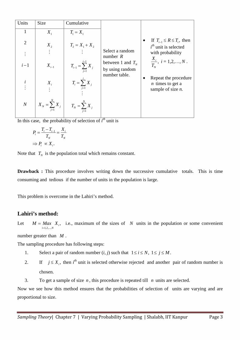
Units Size Cumulative Select a random number R between 1 and NT by using random number table.
• 1If ,i iT R T− ≤ ≤ then ith unit is selected with probability
,i
N
XT
i = 1,2,…, N .
• Repeat the procedure
n times to get a sample of size n.
1 2
1i −
i
N
1X 2X
1iX −
iX
1
N
N jj
X X=
=∑
1 1T X=
2 1 2T X X= +
1
11
i
i jj
T X−
−=
=∑
1
i
i jj
T X=
=∑
1
N
N jj
T X=
=∑
In this case, the probability of selection of ith unit is
1
.
i i ii
N N
i i
T T XPT T
P X
−−= =
⇒ ∝
Note that NT is the population total which remains constant.
Drawback : This procedure involves writing down the successive cumulative totals. This is time
consuming and tedious if the number of units in the population is large.
This problem is overcome in the Lahiri’s method.
Lahiri’s method: Let
1,2,...,,i
i NM Max X
== i.e., maximum of the sizes of N units in the population or some convenient
number greater than M .
The sampling procedure has following steps:
1. Select a pair of random number (i, j) such that 1 , 1 .i N j M≤ ≤ ≤ ≤
2. If ,ij X≤ then ith unit is selected otherwise rejected and another pair of random number is
chosen.
3. To get a sample of size n , this procedure is repeated till n units are selected.
Now we see how this method ensures that the probabilities of selection of units are varying and are
proportional to size.
Sampling Theory| Chapter 7 | Varying Probability Sampling | Shalabh, IIT Kanpur Page 4
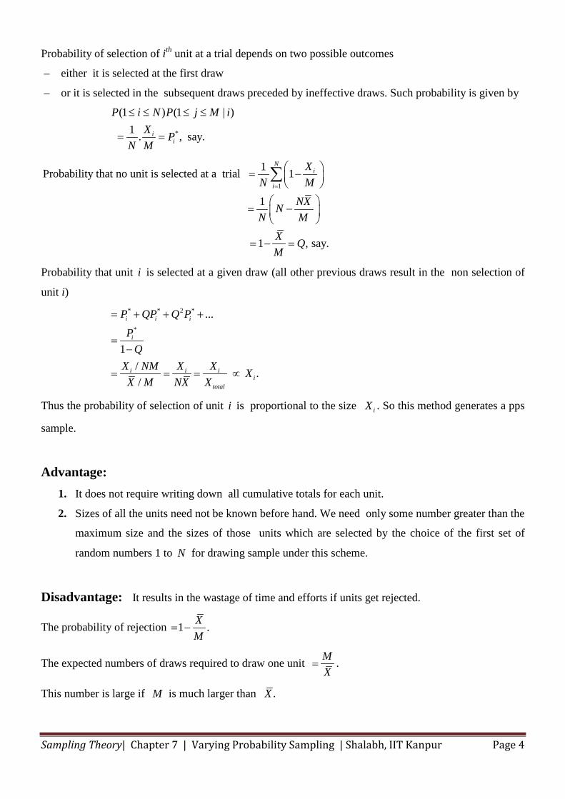
Probability of selection of ith unit at a trial depends on two possible outcomes
– either it is selected at the first draw
– or it is selected in the subsequent draws preceded by ineffective draws. Such probability is given by
*
(1 ) (1 | )1 . , say.i
i
P i N P j M iX P
N M
≤ ≤ ≤ ≤
= =
1
1Probability that no unit is selected at a trial 1
1
1 , say.
Ni
i
XN M
NXNN M
X QM
=
= −
= −
= − =
∑
Probability that unit i is selected at a given draw (all other previous draws result in the non selection of
unit i) * * 2 *
*
...
1/ ./
i i i
i
i i ii
total
P QP Q PP
QX NM X X XX M NX X
= + + +
=−
= = = ∝
Thus the probability of selection of unit i is proportional to the size iX . So this method generates a pps
sample.
Advantage: 1. It does not require writing down all cumulative totals for each unit.
2. Sizes of all the units need not be known before hand. We need only some number greater than the
maximum size and the sizes of those units which are selected by the choice of the first set of
random numbers 1 to N for drawing sample under this scheme.
Disadvantage: It results in the wastage of time and efforts if units get rejected.
The probability of rejection 1 .XM
= −
The expected numbers of draws required to draw one unit MX
= .
This number is large if M is much larger than .X
Sampling Theory| Chapter 7 | Varying Probability Sampling | Shalabh, IIT Kanpur Page 5
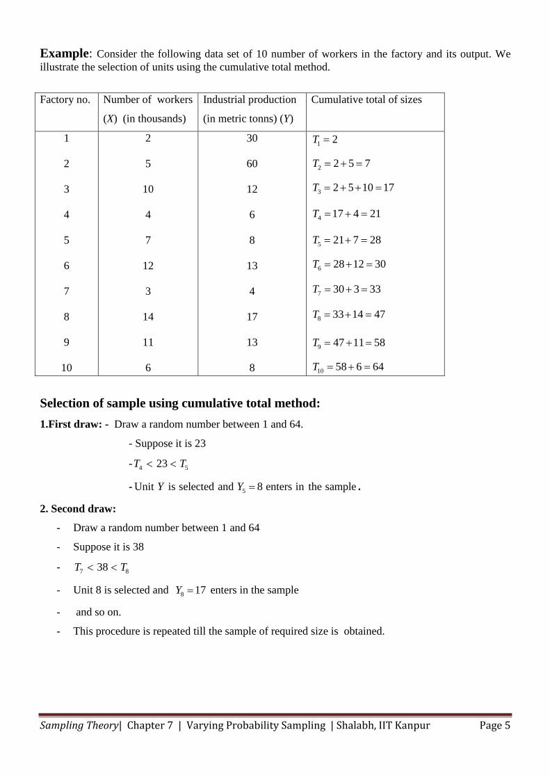
Example: Consider the following data set of 10 number of workers in the factory and its output. We illustrate the selection of units using the cumulative total method.
Factory no. Number of workers
(X) (in thousands)
Industrial production
(in metric tonns) (Y)
Cumulative total of sizes
1 2 3 4 5 6 7 8 9
10
2 5
10 4 7
12 3
14
11 6
30
60
12 6 8
13 4
17
13 8
1 2T =
2 2 5 7T = + =
3 2 5 10 17T = + + =
4 17 4 21T = + =
5 21 7 28T = + =
6 28 12 30T = + =
7 30 3 33T = + =
8 33 14 47T = + =
9 47 11 58T = + =
10 58 6 64T = + =
Selection of sample using cumulative total method: 1.First draw: - Draw a random number between 1 and 64.
- Suppose it is 23
- 4 523T T< <
- 5Unit is selected and 8 enters in the sampleY Y = .
2. Second draw:
- Draw a random number between 1 and 64
- Suppose it is 38
- 7 838T T< <
- Unit 8 is selected and 8 17Y = enters in the sample
- and so on.
- This procedure is repeated till the sample of required size is obtained.
Sampling Theory| Chapter 7 | Varying Probability Sampling | Shalabh, IIT Kanpur Page 6
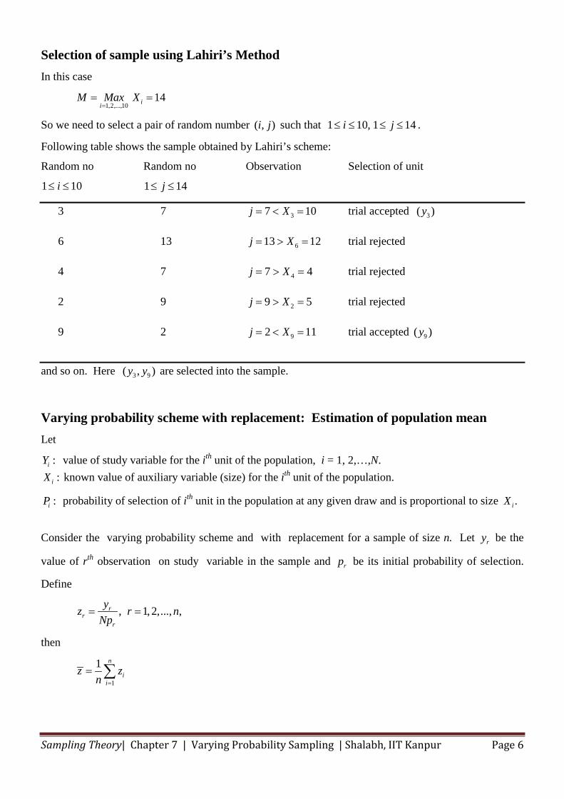
Selection of sample using Lahiri’s Method In this case
1,2,...,10
14iiM Max X
== =
So we need to select a pair of random number ( , )i j such that 1 10, 1 14i j≤ ≤ ≤ ≤ .
Following table shows the sample obtained by Lahiri’s scheme:
Random no Random no Observation Selection of unit
1 10i≤ ≤ 1 14j≤ ≤
3 7 37 10j X= < = trial accepted 3( )y 6 13 613 12j X= > = trial rejected 4 7 47 4j X= > = trial rejected 2 9 29 5j X= > = trial rejected 9 2 92 11j X= < = trial accepted 9( )y
and so on. Here 3 9( , )y y are selected into the sample.
Varying probability scheme with replacement: Estimation of population mean Let
:iY value of study variable for the ith unit of the population, i = 1, 2,…,N. :iX known value of auxiliary variable (size) for the ith unit of the population.
:iP probability of selection of ith unit in the population at any given draw and is proportional to size .iX
Consider the varying probability scheme and with replacement for a sample of size n. Let ry be the
value of rth observation on study variable in the sample and rp be its initial probability of selection.
Define
, 1, 2,..., ,rr
r
yz r nNp
= =
then
1
1 n
ii
z zn =
= ∑
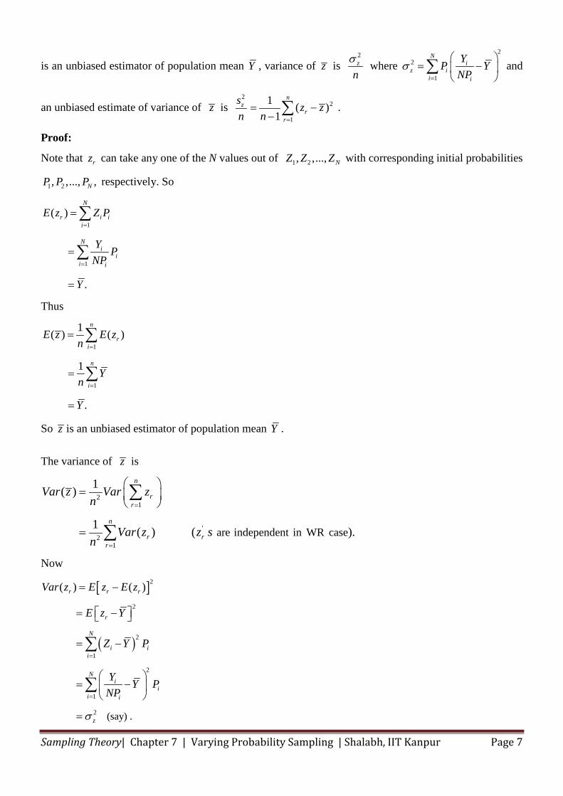
Sampling Theory| Chapter 7 | Varying Probability Sampling | Shalabh, IIT Kanpur Page 7
is an unbiased estimator of population mean Y , variance of z is 2z
nσ where
22
1
Ni
z ii i
YP YNP
σ=
= −
∑ and
an unbiased estimate of variance of z is 2
2
1
1 ( )1
nz
rr
s z zn n =
= −− ∑ .
Proof:
Note that rz can take any one of the N values out of 1 2, ,..., NZ Z Z with corresponding initial probabilities
1 2, ,..., ,NP P P respectively. So
1
1
( )
.
N
r i ii
Ni
ii i
E z Z P
Y PNP
Y
=
=
=
=
=
∑
∑
Thus
1
1
1( ) ( )
1
.
n
ri
n
i
E z E zn
Yn
Y
=
=
=
=
=
∑
∑
So z is an unbiased estimator of population mean Y .
The variance of z is
21
'2
1are independent in WR case
1( )
1 ( ) ( ).
n
rr
n
r rr
Var z Var zn
Var z z sn
=
=
=
=
∑
∑
Now
[ ]
( )
2
2
2
1
2
1
2 (say) .
( ) ( )
r r r
r
N
i ii
Ni
ii i
z
Var z E z E z
E z Y
Z Y P
Y Y PNP
σ
=
=
= −
= −
= −
= −
=
∑
∑
Sampling Theory| Chapter 7 | Varying Probability Sampling | Shalabh, IIT Kanpur Page 8
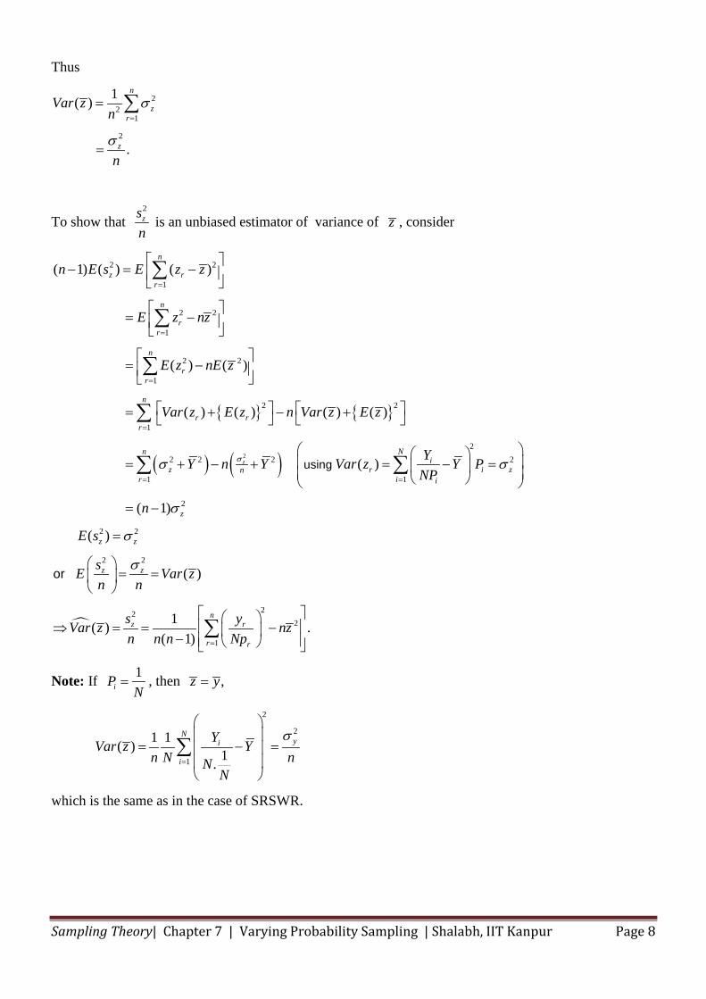
Thus
22
1
2
1( )
.
n
zr
z
Var zn
n
σ
σ
=
=
=
∑
To show that 2zs
n is an unbiased estimator of variance of z , consider
{ } { }
( ) ( )2
2 2
1
2 2
1
2 2
1
2 2
1
22 2 2 2
1 1
2
2
( 1) ( ) ( )
( ) ( )
( ) ( ) ( ) ( )
( )
( 1)
( )
z
n
z rr
n
rr
n
rr
n
r rr
n Ni
z r i znr i i
z
z
n E s E z z
E z nz
E z nE z
Var z E z n Var z E z
YY n Y Var z Y PNP
n
E s
σσ σ
σ
=
=
=
=
= =
− = −
= −
= −
= + − +
= + − + = − =
= −
∑
∑
∑
∑
∑ ∑using
2
2 2
222
1
( )
1( ) .( 1)
z
z z
nz r
r r
sE Var zn n
s yVar z nzn n n Np
σ
σ
=
=
= =
⇒ = = − − ∑
or
Note: If 1iP
N= , then ,z y=
2
2
1
1 1( ) 1.
Nyi
i
YVar z Yn N nN
N
σ
=
= − =
∑
which is the same as in the case of SRSWR.
Sampling Theory| Chapter 7 | Varying Probability Sampling | Shalabh, IIT Kanpur Page 9
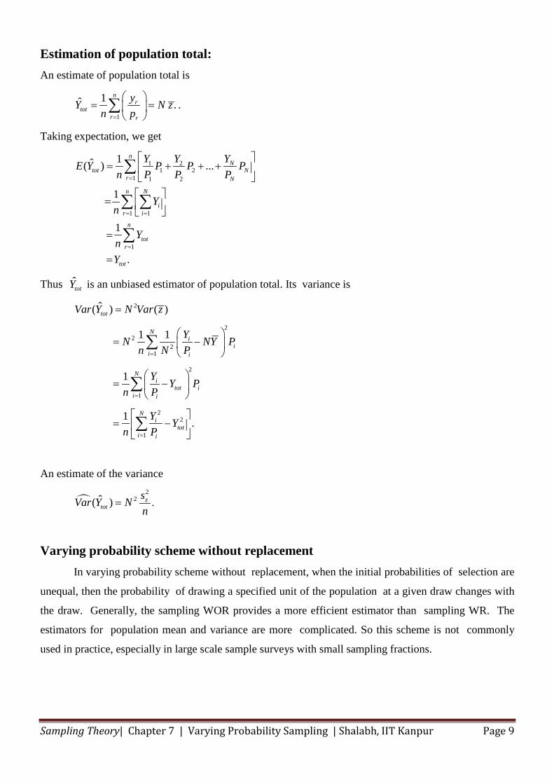
Estimation of population total: An estimate of population total is
1
1ˆ .n
rtot
r r
yY N zn p=
= =
∑ .
Taking expectation, we get
1 21 2
1 1 2
1 1
1
1ˆ( ) ...
1
1
.
nN
tot Nr N
n N
ir i
n
totr
tot
YY YE Y P P Pn P P P
Yn
YnY
=
= =
=
= + + +
=
=
=
∑
∑ ∑
∑
Thus t̂otY is an unbiased estimator of population total. Its variance is
2
22
21
2
1
22
1
ˆ( ) ( )
1 1
1
1 .
tot
Ni
ii i
Ni
tot ii i
Ni
toti i
Var Y N Var z
YN NY Pn N P
Y Y Pn P
Y Yn P
=
=
=
=
= −
= −
= −
∑
∑
∑
An estimate of the variance
22ˆ( ) .z
totsVar Y Nn
=
Varying probability scheme without replacement In varying probability scheme without replacement, when the initial probabilities of selection are
unequal, then the probability of drawing a specified unit of the population at a given draw changes with
the draw. Generally, the sampling WOR provides a more efficient estimator than sampling WR. The
estimators for population mean and variance are more complicated. So this scheme is not commonly
used in practice, especially in large scale sample surveys with small sampling fractions.
Sampling Theory| Chapter 7 | Varying Probability Sampling | Shalabh, IIT Kanpur Page 10
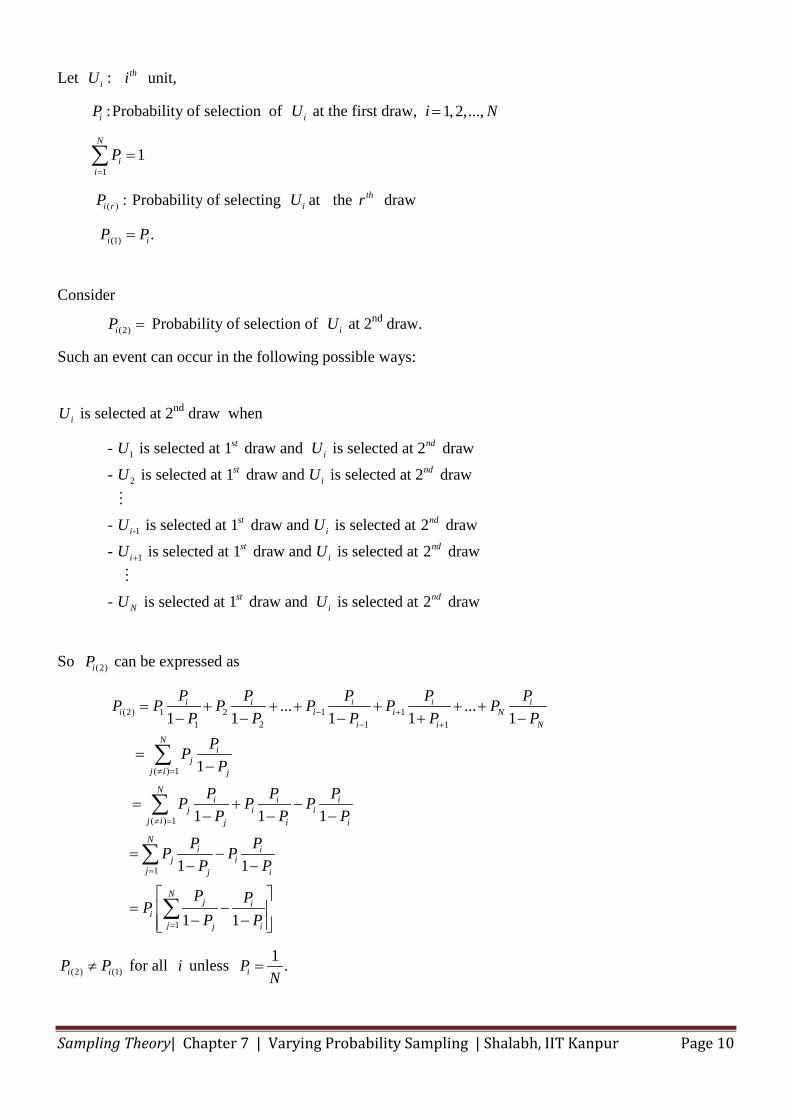
Let :iU thi unit,
:iP Probability of selection of iU at the first draw, i 1,2,..., N=
1
1N
ii
P=
=∑
( ) :i rP Probability of selecting atiU the thr draw
(1) .i iP P=
Consider
(2)iP = Probability of selection of iU at 2nd draw.
Such an event can occur in the following possible ways:
iU is selected at 2nd draw when
1
2
-1
1
- is selected at 1 draw and is selected at 2 draw- is selected at 1 draw and is selected at 2 draw
- is selected at 1 draw and is selected at 2 draw- is selected
st ndi
st ndi
st ndi i
i
U UU U
U UU +
at 1 draw and is selected at 2 draw
- is selected at 1 draw and is selected at 2 draw
st ndi
st ndN i
U
U U
So (2)iP can be expressed as
(2) 1 2 1 11 2 1 1
( ) 1
( ) 1
1
1
... ...1 1 1 1 1
1
1 1 1
1 1
1 1
i i i i ii i i N
i i NN
ij
j i j
Ni i i
j i ij i j i i
Ni i
j ij j i
Nj i
ij j i
P P P P PP P P P P PP P P P P
PPP
P P PP P PP P P
P PP PP P
P PPP P
− +− +
≠ =
≠ =
=
=
= + + + + + +− − − + −
=−
= + −− − −
= −− −
= −
− −
∑
∑
∑
∑
(2) (1)i iP P≠ for all i unless 1 .iPN
=
Sampling Theory| Chapter 7 | Varying Probability Sampling | Shalabh, IIT Kanpur Page 11
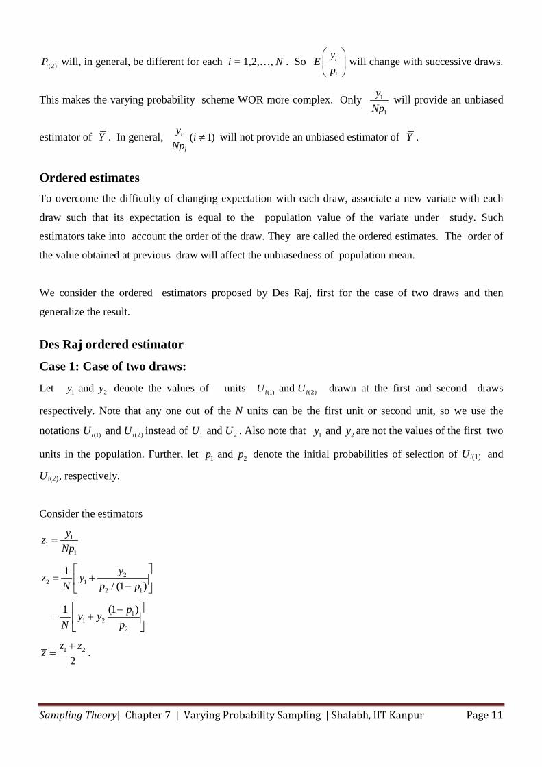
(2)iP will, in general, be different for each i = 1,2,…, N . So i
i
yEp
will change with successive draws.
This makes the varying probability scheme WOR more complex. Only 1
1
yNp
will provide an unbiased
estimator of Y . In general, ( 1)i
i
y iNp
≠ will not provide an unbiased estimator of Y .
Ordered estimates To overcome the difficulty of changing expectation with each draw, associate a new variate with each
draw such that its expectation is equal to the population value of the variate under study. Such
estimators take into account the order of the draw. They are called the ordered estimates. The order of
the value obtained at previous draw will affect the unbiasedness of population mean.
We consider the ordered estimators proposed by Des Raj, first for the case of two draws and then
generalize the result.
Des Raj ordered estimator
Case 1: Case of two draws: Let 1 2andy y denote the values of units (1) (2)andi iU U drawn at the first and second draws
respectively. Note that any one out of the N units can be the first unit or second unit, so we use the
notations (1) (2)andi iU U instead of 1 2andU U . Also note that 1 2andy y are not the values of the first two
units in the population. Further, let 1 2andp p denote the initial probabilities of selection of Ui(1) and
Ui(2), respectively.
Consider the estimators
11
1
22 1
2 1
11 2
2
1 2
1/ (1 )
(1 )1
.2
yzNp
yz yN p p
py yN p
z zz
=
= + −
−= +
+=
Sampling Theory| Chapter 7 | Varying Probability Sampling | Shalabh, IIT Kanpur Page 12
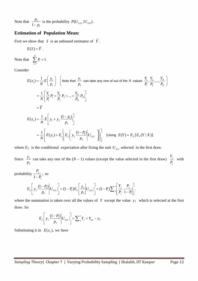
Note that 2
11p
p− is the probability (2) (1)( | ).i iP U U
Estimation of Population Mean:
First we show that z is an unbiased estimator of Y .
( )E z Y= .
Note that 1
1.N
ii
P=
=∑
Consider
1 1 1 21
1 1 1 2
1 21 2
1 2
1( ) , ,...,
1 ...
N
N
NN
N
NYy y Y YE z E
N p p P P P
YY YP P PN P P P
Y
=
= + + +
=
Note that can take any one of out of the values
12 1 2
2
11 1 2 2 (1)
2
(1 )1( )
(1 )1 ( ) ( ( ) [ ( | )].i X Y
pE z E y yN p
PE y E E y U E Y E E Y XN p
−= +
− = + = Using
where E2 is the conditional expectation after fixing the unit (1)iU selected in the first draw.
Since 2
2
yp
can take any one of the (N – 1) values (except the value selected in the first draw) j
j
YP
with
probability 1
,1
jPP−
so
*1 22 2 (1) 1 2 (1) 1
2 2 1
(1 ) (1 ) (1 ) .1
j ji i j
j
Y PP yE y U P E U Pp p P P
−= − = − −
∑ .
where the summation is taken over all the values of Y except the value y1 which is selected at the first
draw. So
*12 2 (1) 1
2
(1 ) .i j totj
PE y U Y Y yp
−= = −
∑
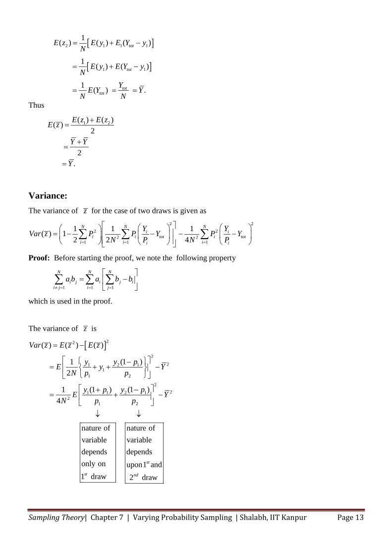
Substituting it in 2( ), we haveE z
Sampling Theory| Chapter 7 | Varying Probability Sampling | Shalabh, IIT Kanpur Page 13
[ ]
[ ]
2 1 1 1
1 1
1( ) ( ) ( )
1 ( ) ( )
1 ( ) .
tot
tot
tottot
E z E y E Y yN
E y E Y yN
YE Y YN N
= + −
= + −
= = =
Thus
1 2( ) ( )( )2
2.
+=
+=
=
E z E zE z
Y Y
Y
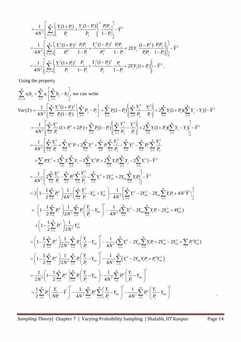
Variance: The variance of z for the case of two draws is given as
2 22 2
2 21 1 1
1 1 1( ) 12 2 4
N N Ni i
i i tot i toti i ii i
Y YVar z P P Y P YN P N P= = =
= − − − −
∑ ∑ ∑
Proof: Before starting the proof, we note the following property
1 1 1
N N N
i j i j ii j i j
a b a b b≠ = = =
= −
∑ ∑ ∑
which is used in the proof.
The variance of z is
[ ]22
2
21 2 11
1 2
221 1 2 1
21 2
( ) ( ) ( )
(1 )1 2
(1 ) (1 )1 4
nature of nature ofvariable variab
depends only on1 draw
= −
−= + + −
+ −= + −
↓ ↓
st
Var z E z E z
y y pE y YN p p
y p y pE YN p p
ledependsupon1 and2 draw
st
nd
Sampling Theory| Chapter 7 | Varying Probability Sampling | Shalabh, IIT Kanpur Page 14
2
22
1
2 22 2 22
2 2 21
2 2
2
(1 )(1 )1 = 4 1
(1 )(1 ) (1 )1 = 24 1 1 1
(1 )1 =4
≠ =
≠ =
−+ + − − −+ − + + − − − −
+
∑
∑
Nj i i ji i
i j i j i
Ni j j i i j i ji i i
i ji j i i j i i j i
i i
Y P PPY P YN P P P
PP Y P PP PPY P PYY YN P P P P PP P
Y PN
2 22
1
(1 )2 (1 ) .
1 1≠ =
− + + + − − − ∑
Nj j i i
i j ii j i i j i
P Y P P YY P YP P P P
Using the property
1 1 1
22 2 22
21 1 1 1 1 1
22
2
, we can write
(1 )1( ) (1 ) 2 (1 )( )]4 (1 )
1 (1 2 ) (14
≠ = = =
= = = = = =
= −
+ = − + − − + + − − −
= + + + −
∑ ∑ ∑
∑ ∑ ∑ ∑ ∑ ∑
N N N
i j i j ii j i j
N N N N N Nji i i
j i i i i i j ii j i j i ji i j i
ii i i
i
a b a b b
YY P YVar z P P P P Y P Y Y YN P P P P
Y P P PN P
2 22
1 1 1 1 1
2 222 2 2 2
21 1 1 1 1 1 1 1
2 2
) 2 (1 )( )
1 24
2 2 2
= = = = =
= = = = = = = =
− + + − −
= + + + − −
+ + − +
∑ ∑ ∑ ∑ ∑
∑ ∑ ∑ ∑ ∑ ∑ ∑ ∑
N N N N Nj i
i i i j ii i j i jj i
N N N N N N N Nj ji
i i i i ii i i i j i i ji j j
i i i j i i i
Y YP Y P Y Y YP P
Y YY Y P Y P Y PN P P P
PY Y Y Y P Y P 2 2
1 1 1 1 1 1
222 2 2 2
21 1 1 1 1
22 2 2 2
2 21 1 1
2 ]
1 2 2 24
1 1 1 2 1 22 4 4
= = = = = =
= = = = =
= = =
− −
= − − + + −
= − − + − −
∑ ∑ ∑ ∑ ∑ ∑ ∑
∑ ∑ ∑ ∑ ∑
∑ ∑ ∑
N N N N N N
i j ii i j i i j i
N N N N Nji
i i tot tot i ii i j i ii j
N N Ni
i tot tot ii i ii
Y Y Y
YY P Y Y Y Y P YN P P
YP Y Y Y YN P N
2 2 2
1
22 2 2 2
2 21 1 1 1
2 22
1
2
1
2 4
1 1 1 1 ( 2 2 4 )2 2 4
1 1 12 2
1 12
=
= = = =
=
=
− +
= − − − − − + + −
= −
∑
∑ ∑ ∑ ∑
∑
∑
N
tot tot i ii
N N N Ni
i i tot i tot i i tot toti i i ii
N
i toti
N
ii
Y Y P N Y
YP P Y Y Y Y P Y YN P N
P YN
P
( )
22 2 2 2 2
2 21 1 1
22 2 2 2
2 21 1 1
22
1
1 1 ( 2 2 2 )2 4
1 1 1 1 22 2 4
1 1 12 2
= = =
= = =
=
− − − + − +
= − − − − +
= −
∑ ∑ ∑ ∑
∑ ∑ ∑
∑
N N Ni
i tot i tot i i tot tot i toti i i ii
N N Ni
i i tot i tot i i i toti i ii
N
ii
YP Y Y Y Y P Y Y P YN P N
YP P Y Y Y Y P P YN P N
PN
22
21 1
2 2 22 2
2 21 1 1 1
14
1 1 1 2 4 4
= =
= = = =
− − −
= − − − − −
∑ ∑
∑ ∑ ∑ ∑
N Ni i
i tot i toti ii i
N N N Ni i i
i i tot i toti i i ii i i
Y YP Y P YP N P
Y Y YP Y P Y P YNP N P N P `
Sampling Theory| Chapter 7 | Varying Probability Sampling | Shalabh, IIT Kanpur Page 15
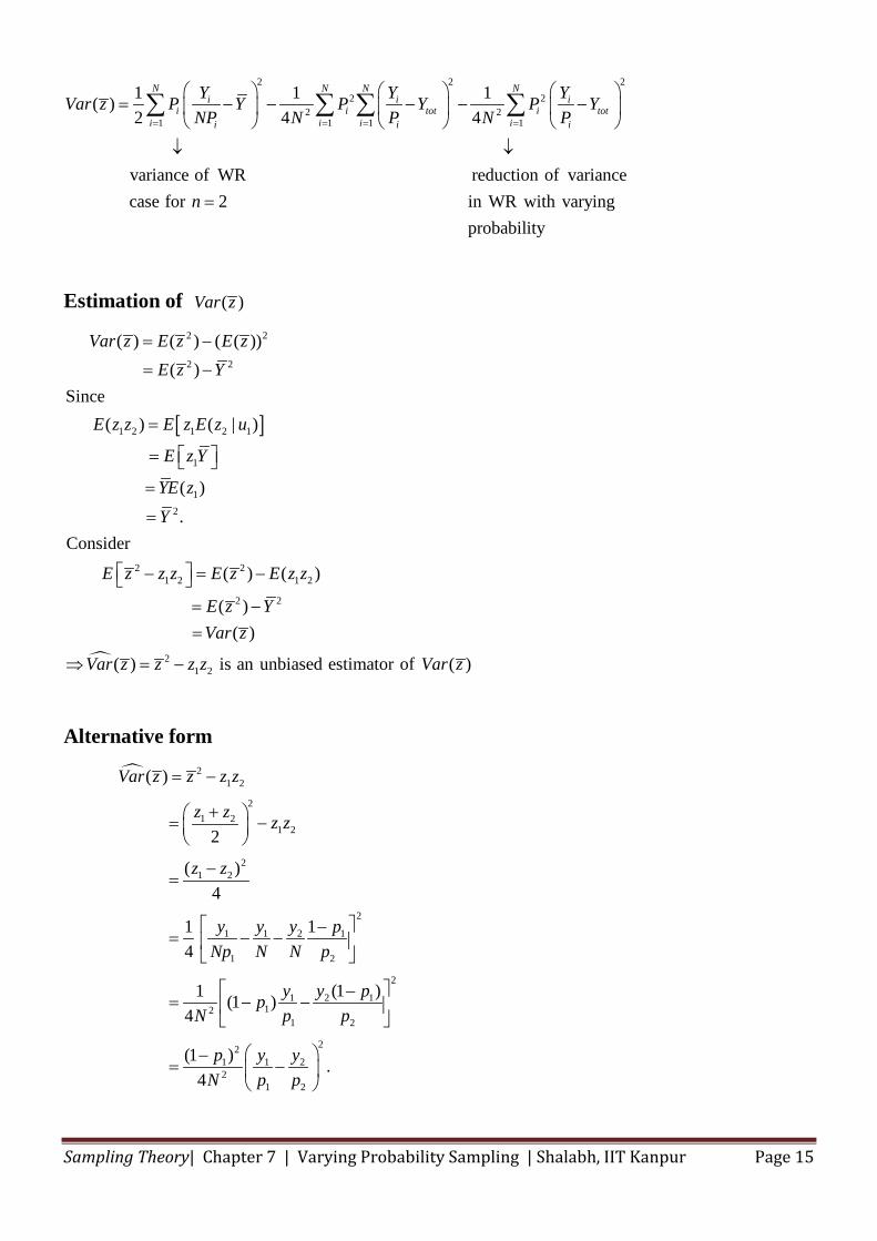
2 2 22 2
2 21 1 1 1
1 1 1( )2 4 4
variance of WR reduction of variancecase for 2 in WR with varying
probability
= = = =
= − − − − −
↓ ↓
=
∑ ∑ ∑ ∑N N N N
i i ii i tot i tot
i i i ii i i
Y Y YVar z P Y P Y P YNP N P N P
n
Estimation of ( )Var z
[ ]
2 2
2 2
1 2 1 2 1
1
12
2 21 2 1 2
2 2
21 2
( ) ( ) ( ( )) ( )Since ( ) ( | )
( ) .
Consider
( ) ( )
( ) ( )
( ) is an unbiased e
Var z E z E zE z Y
E z z E z E z u
E z Y
YE zY
E z z z E z E z z
E z YVar z
Var z z z z
= −
= −
=
= =
=
− = − = −=
⇒ = − stimator of ( )Var z
Alternative form
21 2
21 2
1 2
21 2
2
1 1 2 1
1 2
2
1 2 112
1 2
221 1 22
1 2
( )
2
( )4
114
(1 )1 (1 )4
(1 ) .4
Var z z z z
z z z z
z z
y y y pNp N N p
y y ppN p p
p y yN p p
= −
+ = −
−=
−= − −
−= − −
−= −
Sampling Theory| Chapter 7 | Varying Probability Sampling | Shalabh, IIT Kanpur Page 16
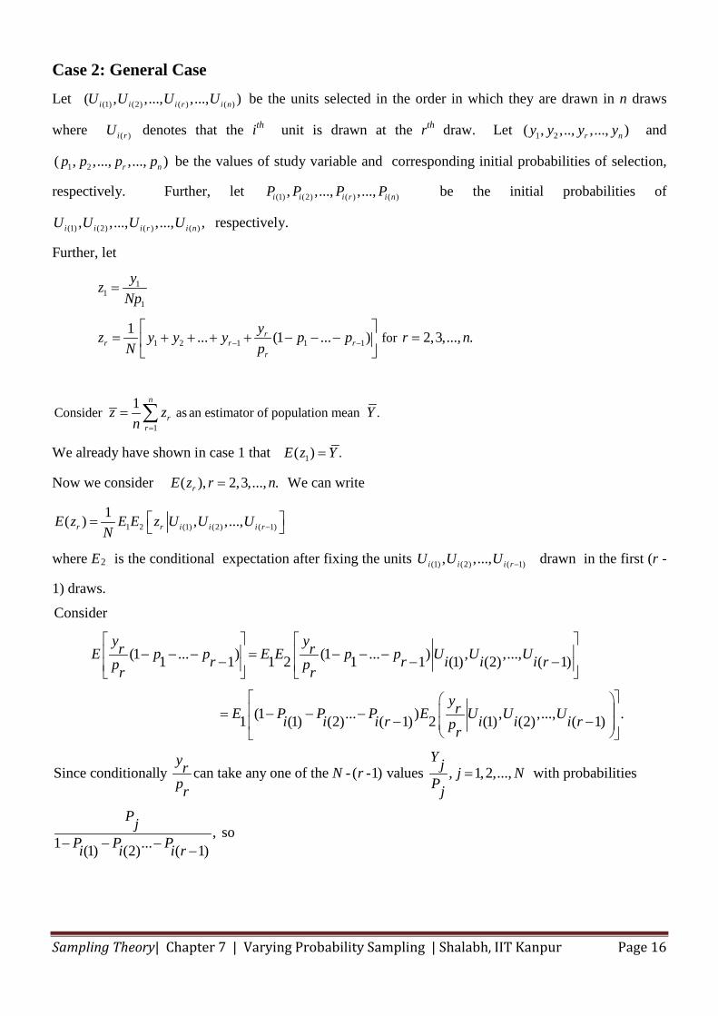
Case 2: General Case Let (1) (2) ( ) ( )( , ,..., ,..., )i i i r i nU U U U be the units selected in the order in which they are drawn in n draws
where ( )i rU denotes that the ith unit is drawn at the rth draw. Let 1 2( , ,.., ,..., )r ny y y y and
1 2( , ,..., ,..., )r np p p p be the values of study variable and corresponding initial probabilities of selection,
respectively. Further, let (1) (2) ( ) ( ), ,..., ,...,i i i r i nP P P P be the initial probabilities of
(1) (2) ( ) ( ), ,..., ,..., ,i i i r i nU U U U respectively.
Further, let
11
1
1 2 1 1 1
1
for
Consider as an estimator of population mean .
1 ... (1 ... ) 2,3,..., .
1
rr r r
r
n
rr
yzNp
yz y y y p p r nN p
z z Yn
− −
=
=
= + + + + − − − =
= ∑
We already have shown in case 1 that 1( )E z Y= .
Now we consider ( ), 2,3,..., .rE z r n= We can write
1 2 (1) (2) ( 1)1( ) , ,...,r r i i i rE z E E z U U UN −
=
where E2 is the conditional expectation after fixing the units (1) (2) ( 1), ,...,i i i rU U U − drawn in the first (r -
1) draws.
Consider
(1 ... ) (1 ... ) , ,...,1 1 1 2 1 1 (1) (2) ( 1)
(1 ... ) ,1 (1) (2) ( 1) 2 (1)
− − − = − − −− − −
= − − − −
y yr rE p p E E p p U U Ur r i i i rp pr r
yrE P P P E U Ui i i r i ipr,..., .(2) ( 1)
Since conditionally can take any one of the - ( -1) values , 1,2,..., with probabilities
, so1 ...(1) (2) ( 1)
−
=
− − − −
Ui r
Yy jr N r j Np Pr j
PjP P Pi i i r
Sampling Theory| Chapter 7 | Varying Probability Sampling | Shalabh, IIT Kanpur Page 17
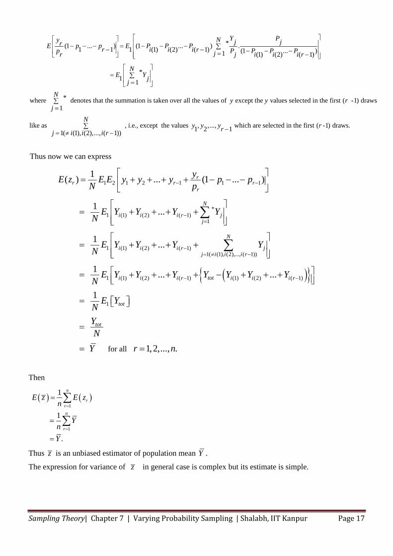
* (1 ... ) (1 ... ) .1 1 1 (1) (2) ( 1) (1 ... )1 (1) (2) ( 1)
* 1 1
*where deno1
Y Py N j jrE p p E P P Pr i i i rp P P P Pjr j i i i r
NE Y jj
N
j
− − − = − − − ∑− − − − −= −
= ∑=
∑=
tes that the summation is taken over all the values of except the values selected in the first ( -1) draws
like as , i.e., except the values , ,..., which 1 2 11( (1), (2),..., ( 1))
y y r
Ny y yrj i i i r
∑ −= ≠ −are selected in the first ( -1) draws. r
1 2 1 2 1 1 1
*1 (1) (2) ( 1)
1
1 (1) (2) (
Thus now we can express
1 ( ) ... (1 ... )
1 ...
1 ...
rr r r
r
N
ji i i rj
i i i r
yE z E E y y y p pN p
E Y Y Y YN
E Y Y YN
− −
−=
−
= + + + + − − −
= + + + +
= + + +
∑
( ){ }
1)1( (1), (2),..., ( 1))
1 (1) (2) ( 1) (1) (2) ( 1)
1
1 ... ...
1
N
jj i i i r
toti i i r i i i r
tot
tot
Y
E Y Y Y Y Y Y YN
E YNYN
= ≠ −
− −
+
= + + + + − + + +
=
=
∑
for all 1,2,..., .Y r n= =
Then
( ) ( )1
1
1
1
.
n
rrn
r
E z E zn
YnY
=
=
=
=
=
∑
∑
Thus z is an unbiased estimator of population mean Y .
The expression for variance of z in general case is complex but its estimate is simple.
Sampling Theory| Chapter 7 | Varying Probability Sampling | Shalabh, IIT Kanpur Page 18
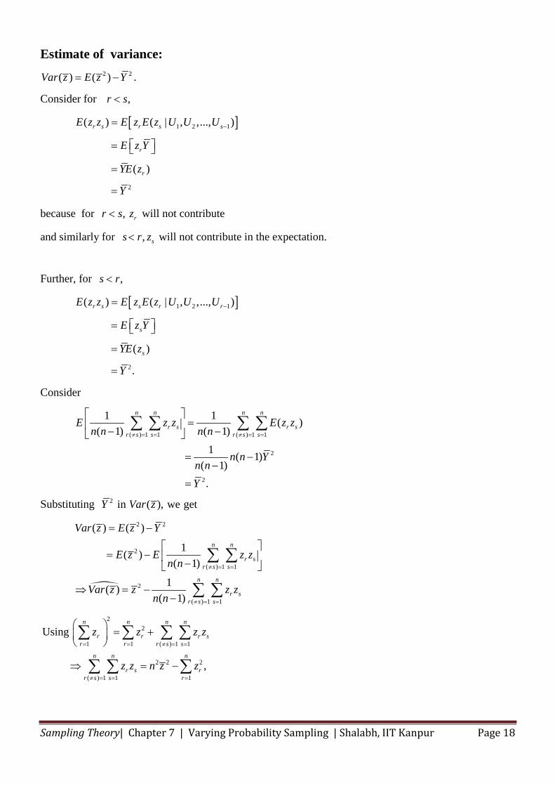
Estimate of variance: 2 2( ) ( )Var z E z Y= − .
Consider for ,r s<
[ ]1 2 1
2
( ) ( | , ,..., )
( )
r s r s s
r
r
E z z E z E z U U U
E z Y
YE z
Y
−=
=
=
=
because for , rr s z< will not contribute
and similarly for , ss r z< will not contribute in the expectation.
Further, for ,s r<
[ ]1 2 1
2
( ) ( | , ,..., )
( )
.
r s s r r
s
s
E z z E z E z U U U
E z Y
YE z
Y
−=
=
=
=
Consider
( ) 1 1 ( ) 1 1
2
2
1 1 ( )( 1) ( 1)
1 ( 1)( 1)
.
n n n n
r s r sr s s r s s
E z z E z zn n n n
n n Yn nY
≠ = = ≠ = =
= − −
= −−
=
∑ ∑ ∑ ∑
Substituting 2 in ( ), we getY Var z
2 2
2
( ) 1 1
2
( ) 1 1
( ) ( )
1 ( )( 1)
1( )( 1)
≠ = =
≠ = =
= −
= − −
⇒ = −−
∑ ∑
∑ ∑
n n
r sr s s
n n
r sr s s
Var z E z Y
E z E z zn n
Var z z z zn n
22
1 1 ( ) 1 1
2 2 2
( ) 1 1 1
Using
,
n n n n
r r r sr r r s s
n n n
r s rr s s r
z z z z
z z n z z
= = ≠ = =
≠ = = =
= +
⇒ = −
∑ ∑ ∑ ∑
∑ ∑ ∑
Sampling Theory| Chapter 7 | Varying Probability Sampling | Shalabh, IIT Kanpur Page 19
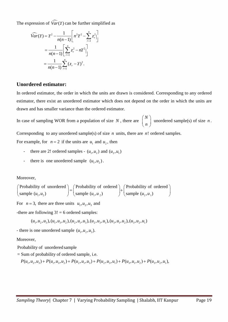
The expression of ( )Var z can be further simplified as
2 2 2 2
1
2 2
1
2
1
1( )( 1)
1( 1)1 ( ) .
( 1)
n
rr
n
rr
n
rr
Var z z n z zn n
z nzn n
z zn n
=
=
=
= − − − = − −
= −−
∑
∑
∑
Unordered estimator: In ordered estimator, the order in which the units are drawn is considered. Corresponding to any ordered
estimator, there exist an unordered estimator which does not depend on the order in which the units are
drawn and has smaller variance than the ordered estimator.
In case of sampling WOR from a population of size N , there are Nn
unordered sample(s) of size n .
Corresponding to any unordered sample(s) of size n units, there are !n ordered samples.
For example, for 2n = if the units are 1 2andu u , then
- there are 2! ordered samples - 1 2 2 1( , ) and ( , )u u u u
- there is one unordered sample 1 2( , )u u .
Moreover,
1 2 1 2 2 1
Probability of unordered Probability of ordered Probability of orderedsample ( , ) sample ( , ) sample ( , )u u u u u u
= +
For 3,n = there are three units 1 2 3, ,u u u and
-there are following 3! = 6 ordered samples:
1 2 3 1 3 2 2 1 3 2 3 1 3 1 2 3 2 1( , , ), ( , , ), ( , , ), ( , , ), ( , , ), ( , , )u u u u u u u u u u u u u u u u u u
- there is one unordered sample 1 2 3( , , ).u u u
Moreover,
1 2 3 1 3 2 2 1 3 2 3 1 3 1 2 3 2 1
Probability of unorderedsample = Sum of probability of ordered sample, i.e. ( , , ) ( , , ) ( , , ) ( , , ) ( , , ) ( , , ),P u u u P u u u P u u u P u u u P u u u P u u u+ + + + +
Sampling Theory| Chapter 7 | Varying Probability Sampling | Shalabh, IIT Kanpur Page 20
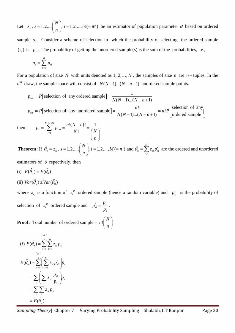
Let , 1, 2,.., , 1, 2,..., !( )si
Nz s i n M
n
= = =
be an estimator of population parameter θ based on ordered
sample is . Consider a scheme of selection in which the probability of selecting the ordered sample
( )is is sip . The probability of getting the unordered sample(s) is the sum of the probabilities, i.e.,
1
.M
s sii
p p=
=∑
For a population of size N with units denoted as 1, 2,…, N , the samples of size n are n − tuples. In the
nth draw, the sample space will consist of ( 1)...( 1)N N N n− − + unordered sample points.
[ ]
[ ]
1selection of any ordered sample( 1)...( 1)
selection of any!selection of any unordered sample !ordered sample( 1)...( 1)
sio
siu
p PN N N n
np P n PN N N n
= =− − +
= = = − − +
then ( !)
1
!( )! 1 .!
M n
s sioi
n N np pNNn
=
=
−= = =
∑
01
ˆ ˆ: If , 1, 2,..., ; 1, 2,..., ( !) and=
′= = = = =
∑TheoremM
si u si sii
Nz s i M n z p
nθ θ are the ordered and unordered
estimators of θ repectively, then
(i) 0ˆ ˆ( ) ( )uE Eθ θ=
(ii) 0ˆ ˆ( ) ( )uVar Varθ θ≤
where isz is a function of th
is ordered sample (hence a random variable) and isp is the probability of
selection of this ordered sample and ′ = si
sis
ppp
.
Proof: Total number of ordered sample = !N
nn
01 1
1 1
0
ˆ( ) ( )
ˆ( )
ˆ( )
= =
= =
=
′=
=
=
=
∑∑
∑ ∑
∑ ∑
∑∑
Nn M
si sis i
Nn M
u si si ss i
sisi s
s i s
si sis i
i E z p
E z p p
pz pp
z p
E
θ
θ
θ
Sampling Theory| Chapter 7 | Varying Probability Sampling | Shalabh, IIT Kanpur Page 21
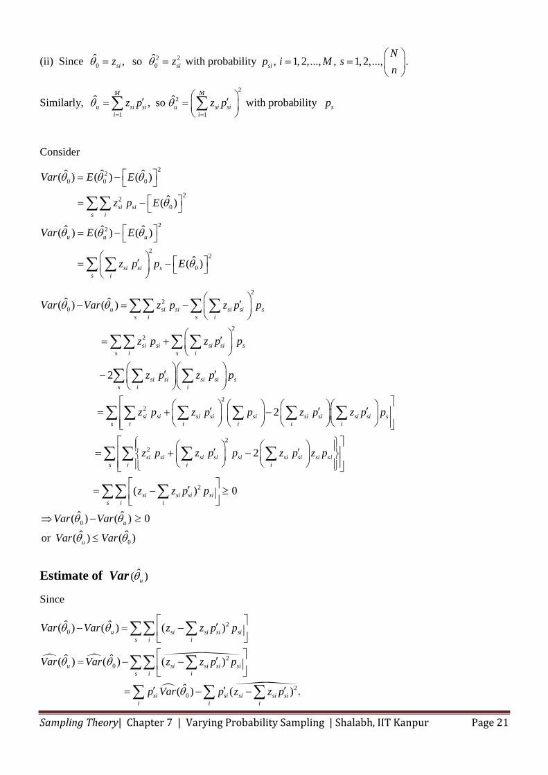
(ii) Since 0̂ ,sizθ = so 2 20̂ sizθ = with probability , 1, 2,..., , 1, 2,...,si
Np i M s
n
= =
.
Similarly, 2
2
1 1
ˆ ˆ, so= =
′ ′= =
∑ ∑M M
u si si u si sii i
z p z pθ θ with probability sp
Consider 22
0 0 0
220
22
22
0
ˆ ˆ ˆ( ) ( ) ( )
ˆ ( )
ˆ ˆ ˆ( ) ( ) ( )
ˆ ( )
= −
= −
= −
′= −
∑∑
∑ ∑
si sis i
u u u
si si ss i
Var E E
z p E
Var E E
z p p E
θ θ θ
θ
θ θ θ
θ
22
0
22
22
ˆ ˆ( ) ( )
2
2
′− = −
′= +
′ ′−
′ ′ ′= + −
∑∑ ∑ ∑
∑∑ ∑ ∑
∑ ∑ ∑
∑ ∑ ∑ ∑ ∑
u si si si si ss i s i
si si si si ss i s i
si si si si ss i i
si si si si si si si si si ss i i i i i
Var Var z p z p p
z p z p p
z p z p p
z p z p p z p z p p
θ θ
22
2
0
0
2
( ) 0
ˆ ˆ( ) ( ) 0ˆ ˆor ( ) ( )
′ ′ = + − ′= − ≥
⇒ − ≥
≤
∑
∑ ∑ ∑ ∑
∑∑ ∑
si si si si si si si si sis i i i
si si si sis i i
u
u
z p z p p z p z p
z z p p
Var Var
Var Var
θ θ
θ θ
Estimate of Var ˆ( )uθ
Since
20
20
20
ˆ ˆ( ) ( ) ( )
ˆ ˆ( ) ( ) ( )
ˆ( ) ( ) .
′− = − ′= − −
′ ′ ′= − −
∑∑ ∑
∑∑ ∑
∑ ∑ ∑
u si si si sis i i
u si si si sis i i
si si si si sii i i
Var Var z z p p
Var Var z z p p
p Var p z z p
θ θ
θ θ
θ
Sampling Theory| Chapter 7 | Varying Probability Sampling | Shalabh, IIT Kanpur Page 22
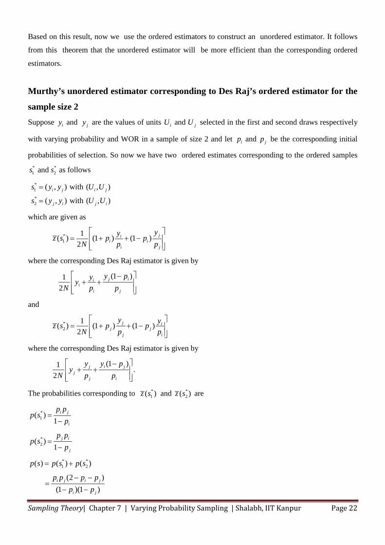
Based on this result, now we use the ordered estimators to construct an unordered estimator. It follows
from this theorem that the unordered estimator will be more efficient than the corresponding ordered
estimators.
Murthy’s unordered estimator corresponding to Des Raj’s ordered estimator for the
sample size 2 Suppose andi jy y are the values of units andi jU U selected in the first and second draws respectively
with varying probability and WOR in a sample of size 2 and let andi jp p be the corresponding initial
probabilities of selection. So now we have two ordered estimates corresponding to the ordered samples * *1 2and s s as follows
*1
*2
( , ) with ( , )
( , ) with ( , )i j i j
j i j i
s y y U U
s y y U U
=
=
which are given as
*1
1( ) (1 ) (1 )2
jii i
i j
yyz s p pN p p
= + + −
where the corresponding Des Raj estimator is given by
(1 )1
2j ii
ii j
y pyyN p p −
+ +
and
*2
1( ) (1 ) (1 )2
j ij j
j i
y yz s p pN p p
= + + −
where the corresponding Des Raj estimator is given by
(1 )1 .2
j i jj
j i
y y py
N p p −
+ +
The probabilities corresponding to *1( )z s and *
2( )z s are
*1
*2
* *1 2
( )1
( )1
( ) ( ) ( )
(2 )(1 )(1 )
i j
i
j i
j
i j i j
i j
p pp s
p
p pp s
p
p s p s p s
p p p pp p
=−
=−
= +
− −=
− −
Sampling Theory| Chapter 7 | Varying Probability Sampling | Shalabh, IIT Kanpur Page 23
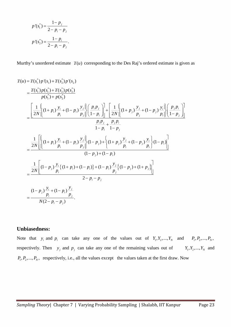
*1
*2
1'( )
2
1'( ) .2
j
i j
i
i j
pp s
p p
pp sp p
−=
− −
−=
− −
Murthy’s unordered estimate ( )z u corresponding to the Des Raj’s ordered estimate is given as
* *1 1 2 2
* * * *1 1 2 2
* *1 2
( ) ( ) '( ) ( ) '( )
( ) ( ) ( ) ( )( ) ( )
1 1(1 ) (1 ) (1 ) (1 )2 1 2 1
1 1
j i j j j ii ii i j j
i j i j i j
i j j i
i
z u z s p s z s p s
z s p s z s p sp s p s
y p p y p py yp p p pN p p p N p p p
p p p pp
= +
+=
+
+ + − + + + − − − =+
− −
{ } { }
1 (1 ) (1 ) (1 ) (1 ) (1 ) (1 )2
(1 ) (1 )
1 (1 ) (1 ) (1 ) (1 ) (1 ) (12
2
(1 ) (1 ).
(2 )
j
j ji ii i j j j i
i j i i
j i
jij i i i j j
i j
i j
jij i
i j
i j
p
y yy yp p p p p pN p p p p
p p
yyp p p p p pN p p
p p
yyp pp p
N p p
+ + − − + + + − − =
− + −
− + + − + − − + +
=− −
− + −=
− −
Unbiasedness: Note that andi iy p can take any one of the values out of 1 2, ,..., NY Y Y and 1 2, ,..., ,NP P P
respectively. Then andj jy p can take any one of the remaining values out of 1 2, ,..., NY Y Y and
1 2, ,..., ,NP P P respectively, i.e., all the values except the values taken at the first draw. Now

Sampling Theory| Chapter 7 | Varying Probability Sampling | Shalabh, IIT Kanpur Page 24
[ ](1 ) (1 )
1 11( )2
(1 ) (1 )1 11 2
2 2
(11
2
j i j i jij i
i j i j
i j i j
j i j j iij i
i j i j
i j i j
Y PP PPYP PP P P P
E z uN P P
Y PP P PYP PP P P P
N P P
N
<
<
− + − + − − =− −
− + − + − − =− −
−
=
∑
∑
) (1 )
1 1
2
1 (1 ) (1 )2 (1 )(1 )
12 1 1
j i j j iij i
i j i j
i j i j
j i jij i
i j i j i j
i j j i
i j i j
Y PP P PYP PP P P P
P P
Y PPYP PN P P P P
Y P Y PN P P
≠
≠
≠
+ − + − − − −
= − + − − −
= +
− −
∑
∑
∑
Using result 1 1 1
,N N N
i j i j ii j i j
a b a b b≠ = = =
= −
∑ ∑ ∑ we have
[ ]1 1 1 1
1 1
1 1
1( ) ( ) ( )2 1 1
1 (1 ) (1 )2 1 1
12
2
N N N Nji
j i i ji j j ii j
N Nji
i ji ji j
N N
i ji j
YYE z u P P P PN P P
YY P PN P P
Y YN
Y Y
= = = =
= =
= =
= − + − − −
= − + − − −
= +
+=
∑ ∑ ∑ ∑
∑ ∑
∑ ∑
.Y=
Sampling Theory| Chapter 7 | Varying Probability Sampling | Shalabh, IIT Kanpur Page 25
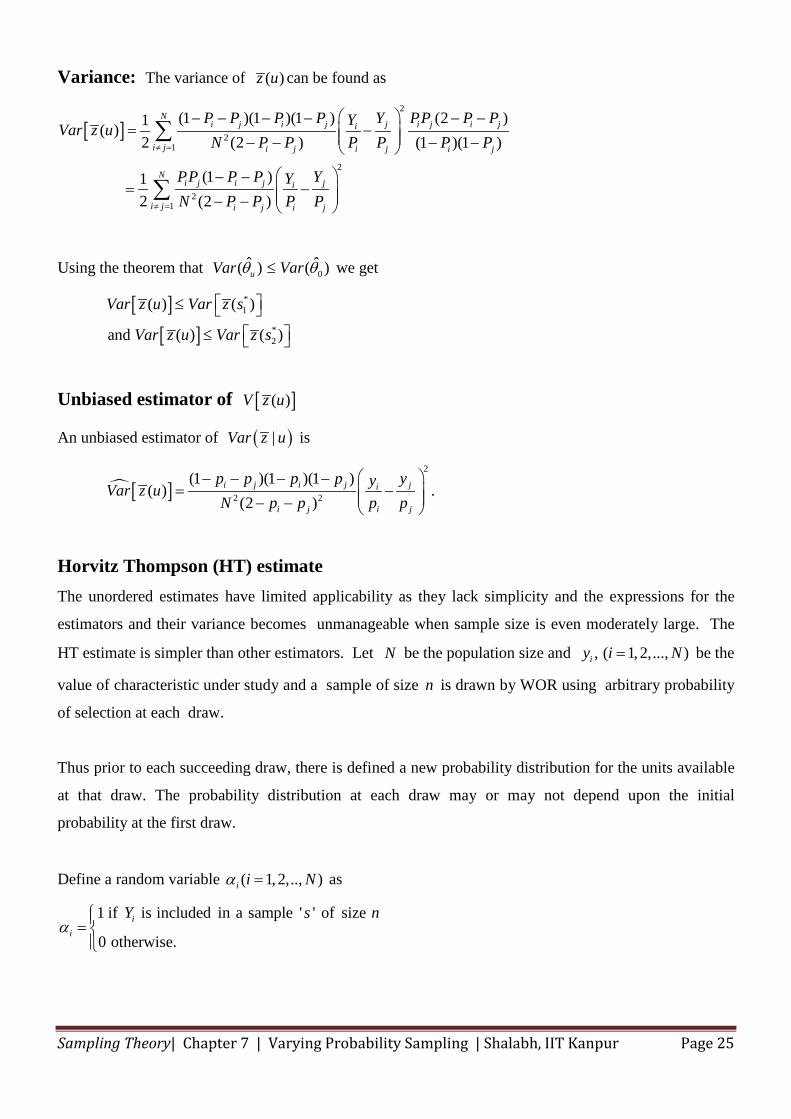
Variance: The variance of ( )z u can be found as
[ ]2
21
2
21
(1 )(1 )(1 ) (2 )1( )2 (2 ) (1 )(1 )
(1 )12 (2 )
Ni j i j j i j i ji
i j i j i j i j
Ni j i j ji
i j i j i j
P P P P Y PP P PYVar z uN P P P P P P
PP P P YYN P P P P
≠ =
≠ =
− − − − − −= − − − − −
− −= − − −
∑
∑
Using the theorem that 0ˆ ˆ( ) ( )uVar Varθ θ≤ we get
[ ]
[ ]
*1
*2
( ) ( )
and ( ) ( )
Var z u Var z s
Var z u Var z s
≤ ≤
Unbiased estimator of [ ]( )V z u
An unbiased estimator of ( )|Var z u is
[ ]2
2 2
(1 )(1 )(1 )( ) .
(2 )i j i j ji
i j i j
p p p p yyVar z uN p p p p
− − − −= − − −
Horvitz Thompson (HT) estimate The unordered estimates have limited applicability as they lack simplicity and the expressions for the
estimators and their variance becomes unmanageable when sample size is even moderately large. The
HT estimate is simpler than other estimators. Let N be the population size and , ( 1, 2,..., )iy i N= be the
value of characteristic under study and a sample of size n is drawn by WOR using arbitrary probability
of selection at each draw.
Thus prior to each succeeding draw, there is defined a new probability distribution for the units available
at that draw. The probability distribution at each draw may or may not depend upon the initial
probability at the first draw.
Define a random variable ( 1, 2,.., )i i Nα = as
1 if is included in a sample ' ' of size
0 otherwise.i
i
Y s nα
=
Sampling Theory| Chapter 7 | Varying Probability Sampling | Shalabh, IIT Kanpur Page 26
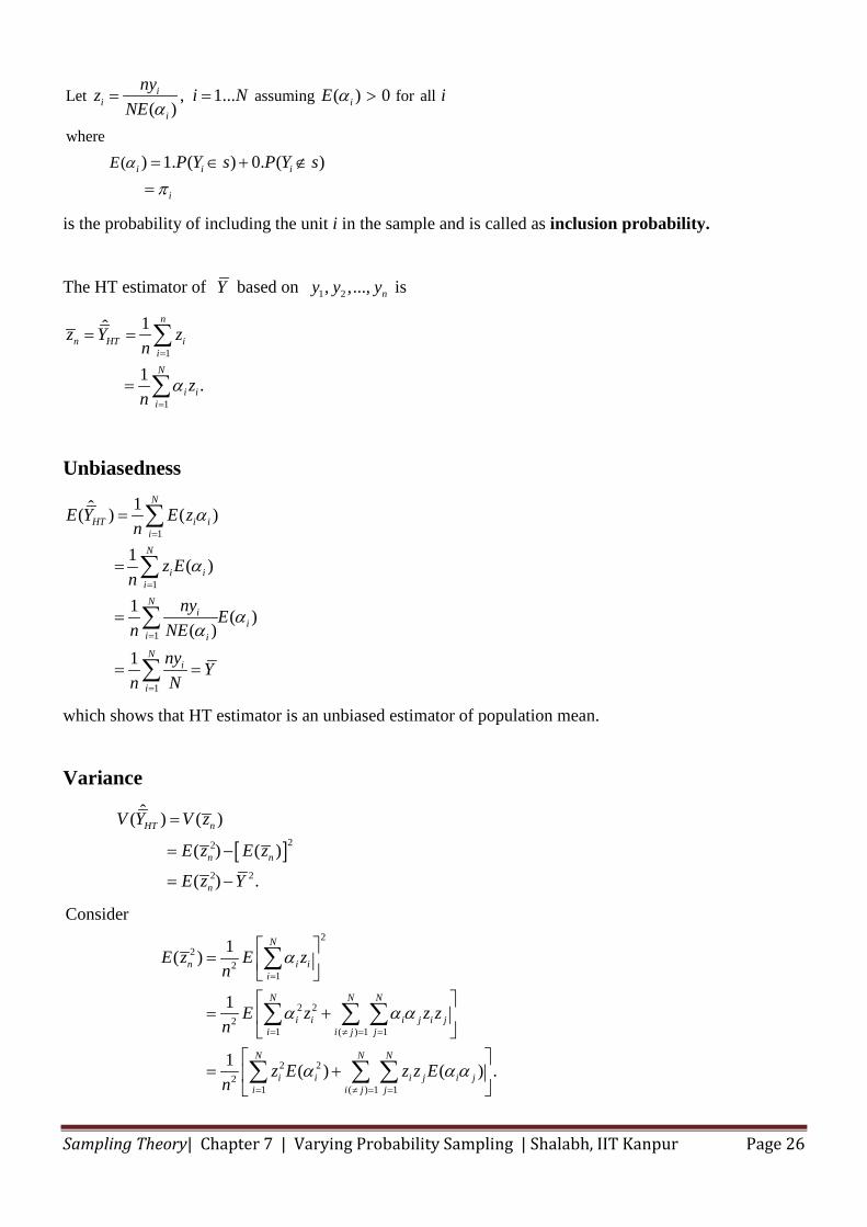
Let assuming for all
where (
, 1... ( ) 0 ( )
) 1. ( ) 0. ( )
ii i
i
i i i
i
E
nyz i N E iNE
P Y s P Y sα
αα
π
= = >
= ∈ + ∉=
is the probability of including the unit i in the sample and is called as inclusion probability.
The HT estimator of Y based on 1 2, ,..., ny y y is
1
1
1ˆ
1 .
n
n HT iiN
i ii
z Y zn
zn
α
=
=
= =
=
∑
∑
Unbiasedness
1
1
1
1
1ˆ( ) ( )
1 ( )
1 ( )( )
1
N
HT i iiN
i iiN
ii
i iN
i
i
E Y E zn
z En
ny En NE
ny Yn N
α
α
αα
=
=
=
=
=
=
=
= =
∑
∑
∑
∑
which shows that HT estimator is an unbiased estimator of population mean.
Variance
[ ]22
2 2
ˆ( ) ( )
( ) ( )
( ) .
HT n
n n
n
V Y V z
E z E z
E z Y
=
= −
= −
22
21
2 22
1 ( ) 1 1
2 22
1 ( ) 1 1
Consider
1( )
1
1 ( ) ( ) .
N
n i ii
N N N
i i i j i ji i j j
N N N
i i i j i ji i j j
E z E zn
E z z zn
z E z z En
α
α α α
α α α
=
= ≠ = =
= ≠ = =
=
= +
= +
∑
∑ ∑ ∑
∑ ∑ ∑
Sampling Theory| Chapter 7 | Varying Probability Sampling | Shalabh, IIT Kanpur Page 27
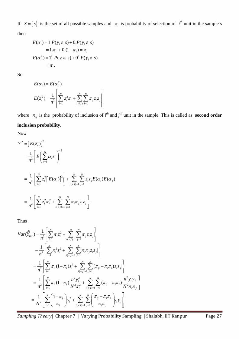
If { }S s= is the set of all possible samples and iπ is probability of selection of ith unit in the sample s
then
2 2 2
( ) 1 ( ) 0. ( )1. 0.(1 )
( ) 1 . ( ) 0 . ( ).
i i i
i i i
i i i
i
E P y s P y s
E P y s P y s
απ π π
απ
= ∈ + ∉= + − =
= ∈ + ∉=
So
2
2 22
1 (# ) 1
( ) ( )
1( )
i i
N N N
n i i ij i ji i j i
E E
E z z z zn
α α
π π= =
=
= + ∑ ∑∑
where ijπ is the probability of inclusion of ith and jth unit in the sample. This is called as second order
inclusion probability.
Now
[ ]
[ ]
22
2
21
222
1 ( ) 1 1
2 22
1 ( ) 1 1
( )
1
1 ( ) ( ) ( )
1 .
n
N
i ii
N N N
i i i j i ji i j j
N N N
i i i j i ji i j j
Y E z
E zn
z E z z E En
z z zn
α
α α α
π π π
=
= ≠ = =
= ≠ = =
=
=
= +
= +
∑
∑ ∑ ∑
∑ ∑ ∑
Thus
22
1 ( ) 1 1
2 22
1 ( ) 1 1
22
1 ( ) 1 1
22 2
2 2 2( ) 1 1
1ˆ( )
1
1 (1 ) ( )
1 (1 ) ( )
N N N
HT i i ij i ji i j j
N N N
i i i j i ji i j j
N N N
i i i ij i i i ji i j j
N Ni
i i ij i ii j ji
Var Y z z zn
z z zn
z z zn
n yn yn N
π π
π π π
π π π π π
π π π π ππ
= ≠ = =
= ≠ = =
= ≠ = =
≠ = =
= +
− +
= − + −
= − + −
∑ ∑ ∑
∑ ∑ ∑
∑ ∑ ∑
∑ ∑ 21
22
1 ( ) 1 1
11
Ni j
i i j
N N Nij i ii
i i ji i j ji i j
yN
y y yN
π π
π π πππ π π
=
= ≠ = =
− −
= +
∑
∑ ∑ ∑
Sampling Theory| Chapter 7 | Varying Probability Sampling | Shalabh, IIT Kanpur Page 28
Estimate of variance
2
1 2 21 ( ) 1 1
(1 )1ˆˆ ( ) .n n n
ij i j i ji iHT
i i j ji i j i j
y yyV Var YN
π π πππ π π π= ≠ = =
−−= = +
∑ ∑ ∑
This is an unbiased estimator of variance .
Drawback: It does not reduces to zero when all i
i
yπ
are same, i.e., when .i iy π∝
Consequently, this may assume negative values for some samples.
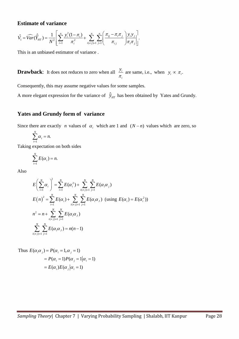
A more elegant expression for the variance of ˆHTy has been obtained by Yates and Grundy.
Yates and Grundy form of variance Since there are exactly n values of iα which are 1 and ( )N n− values which are zero, so
1
.N
ii
nα=
=∑
Taking expectation on both sides
1
( ) .N
ii
E nα=
=∑
Also
( )
22
1 1 ( ) 1 1
2 2
1 ( ) 1 1
2
( ) 1 1
( ) 1 1
( ) ( )
( ) ( ) (using ( ) ( ))
( )
( ) ( 1)
N N N N
i i i ji i i j j
N N N
i i J i ii i j j
N N
i Ji j j
N N
i Ji j j
E E E
E n E E E E
n n E
E n n
α α α α
α α α α α
α α
α α
= = ≠ = =
= ≠ = =
≠ = =
≠ = =
= +
= + =
= +
= −
∑ ∑ ∑ ∑
∑ ∑ ∑
∑ ∑
∑ ∑
Thus ( ) ( 1, 1)
( 1) ( 1 1)
( ) ( 1)
i j i j
i j i
i j i
E P
P P
E E
α α α α
α α α
α α α
= = =
= = = =
= =
Sampling Theory| Chapter 7 | Varying Probability Sampling | Shalabh, IIT Kanpur Page 29
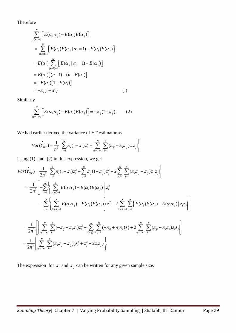
Therefore
[ ][ ]
( ) 1
( ) 1
( ) 1
( ) ( ) ( )
( ) ( | 1) ( ) ( )
( ) ( | 1) ( )
( ) ( 1) ( ( )
( ) 1 ( )(1 ) (1)
N
i j i jj i
N
i j i i jj i
N
i j i jj i
i i
i i
i i
E E E
E E E E
E E E
E n n E
E E
α α α α
α α α α α
α α α α
α α
α απ π
≠ =
≠ =
≠ =
−
= = −
= = −
= − − −
= − −
= − −
∑
∑
∑
Similarly
( ) 1( ) ( ) ( ) (1 ). (2)
N
i j i j j ji j
E E Eα α α α π π≠ =
− = − − ∑
We had earlier derived the variance of HT estimator as
22
1 ( ) 1 1
1ˆ( ) (1 ) ( )N N N
HT i i i ij i j i ji i j j
Var Y z z zn
π π π π π= ≠ = =
= − + −
∑ ∑ ∑
Using (1) and (2) in this expression, we get
2 22
1 1 1 1
22
1 ( ) 1
2
1 ( ) 1
1ˆ( ) (1 ) (1 ) 2 ( )2
1 ( ) ( ) ( )2
( ) ( ) ( ) 2 ( )
N N N N
HT i i i j j j i j ij i ji j i j j
N N
i j i j ii j i
N N
i j i j j ij i j
Var Y z z z zn
E E E zn
E E E z E E
π π π π π π π
α α α α
α α α α α
= = ≠ = =
= ≠ =
= ≠ =
= − + − − −
= − −
− − −
∑ ∑ ∑∑
∑ ∑
∑ ∑ { }( ) 1 1
2 22
( ) 1 1 ( ) 1 1 ( ) 1 1
2 22
( ) 1 1
( ) ( )
1 ( ) ( ) 2 ( )2
1 ( )( 2 ) .2
N n
j i j i ji j j
N N N N N N
ij i i i ij i i j ij i i i ji j j i j j i j j
N N
i j ij i j i ji j j
E z z
z z z zn
z z z zn
α α α
π π π π π π π π π
π π π
≠ = =
≠ = = ≠ = = ≠ = =
≠ = =
−
= − + + − + + −
= − + −
∑ ∑
∑ ∑ ∑ ∑ ∑ ∑
∑ ∑
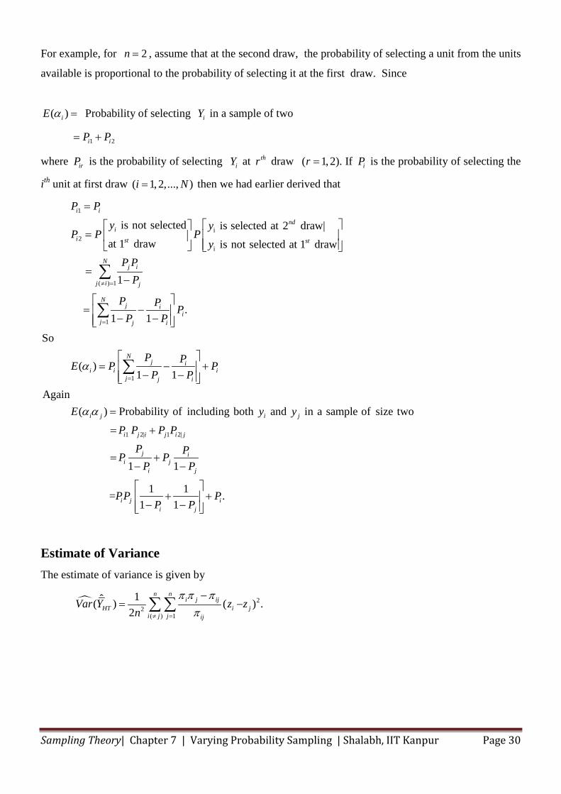
The expression for andi ijπ π can be written for any given sample size.
Sampling Theory| Chapter 7 | Varying Probability Sampling | Shalabh, IIT Kanpur Page 30
For example, for 2n = , assume that at the second draw, the probability of selecting a unit from the units
available is proportional to the probability of selecting it at the first draw. Since
( )iE α = Probability of selecting iY in a sample of two
1 2i iP P= +
where irP is the probability of selecting iY at thr draw ( 1, 2). If ir P= is the probability of selecting the
ith unit at first draw ( 1,2,..., )i N= then we had earlier derived that
1
i2
i
( ) 1
1
is not selected is selected at 2 draw|
at 1 draw is not selected at 1 draw
1
.1 1
So
(
≠ =
=
=
=
=−
= −
− −
∑
∑
i i
ndi
i st st
Nj i
j i j
Nj i
ij j i
i
P P
y yP P P
yP P
P
P P PP P
E α1
1 2| 1 2|
)1 1
Again ( ) Probability of including both and in a sample of size two
1 1
1 1 = .1 1
=
= − +
− −
=
= +
= +− −
+ +
− −
∑N
j ii i
j j i
i j i j
i j i j i j
j ii j
i j
i j ii j
P PP PP P
E y yP P P P
P PP PP P
PP PP P
α α
Estimate of Variance The estimate of variance is given by
22
( ) 1
1ˆ( ) ( ) .2
n ni j ij
HT i ji j j ij
Var Y z zn
π π ππ≠ =
−= −∑∑
Sampling Theory| Chapter 7 | Varying Probability Sampling | Shalabh, IIT Kanpur Page 31
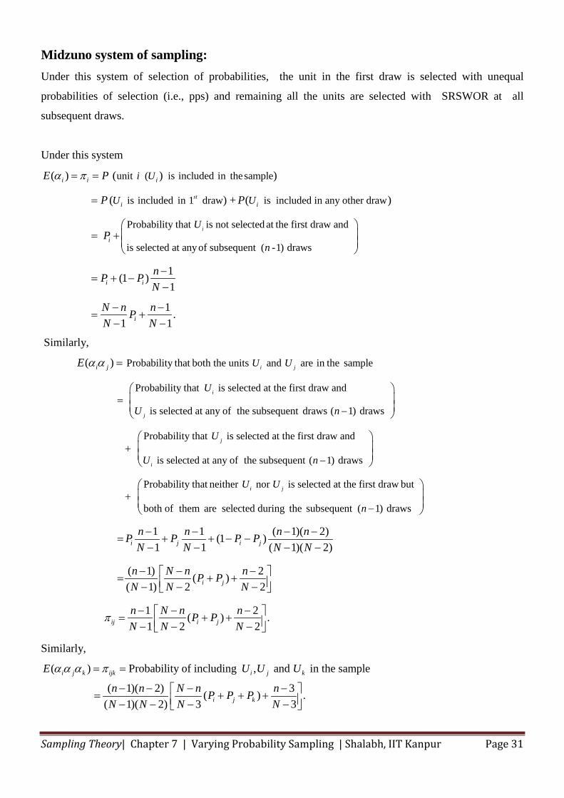
Midzuno system of sampling: Under this system of selection of probabilities, the unit in the first draw is selected with unequal
probabilities of selection (i.e., pps) and remaining all the units are selected with SRSWOR at all
subsequent draws.
Under this system
unit ( is included in thesample
is included in 1 draw is included in any other draw
Probability that is not selected at the first draw and
is selected at any of su
( ) ( ) )
( ) + ( )
st
i
i i i
i i
i
i U
U U
U
E P
P P
P
α π= =
=
= +bsequent ( -1) draws
1 (1 )1
1 .1 1
i i
i
n
nP PN
N n nPN N
−= + −
−
− −= +
− −
Similarly,
Probability that both the units and are in the sample
Probability that is selected at the first draw and
is selected at any of the subsequent draws ( 1) draws
Probabili
( ) i j
i
j
i j U U
U
U n
E α α
=−
+
=
ty that is selected at the first draw and
is selected at any of the subsequent ( 1) draws
Probability that neither nor is selected at the first draw but
both of them a
j
i
i j
U
U n
U U
−
+
re selected during the subsequent ( 1) draws
1 1 ( 1)( 2)(1 )1 1 ( 1)( 2)
( 1) 2( )( 1) 2 2
1 2( ) .1 2 2
i j i j
i j
ij i j
n
n n n nP P P PN N N N
n N n nP PN N N
n N n nP PN N N
π
−
− − − −= + + − −
− − − −
− − − = + + − − −
− − − = + + − − −
Similarly,
( ) Probability of including , and in the sample
( 1)( 2) 3 ( ) .( 1)( 2) 3 3
i j k ijk i j k
i j k
E U U U
n n N n nP P PN N N N
α α α π= =
− − − − = + + + − − − −
Sampling Theory| Chapter 7 | Varying Probability Sampling | Shalabh, IIT Kanpur Page 32
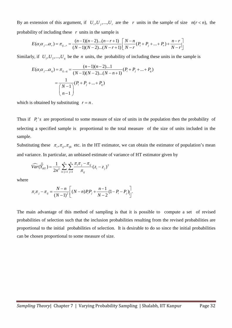
By an extension of this argument, if , ,...,i j rU U U are the r units in the sample of size ( ),n r n< the
probability of including these r units in the sample is
...( 1)( 2)...( 1)( ... ) ( ... )
( 1)( 2)...( 1)i j r ij r i j rn n n r N n n rE P P P
N N N r N r N rα α α π − − − + − − = = + + + + − − − + − −
Similarly, if 1 2, ,..., qU U U be the n units, the probability of including these units in the sample is
...( 1)( 2)...1( ... ) ( ... )
( 1)( 2)...( 1)1 ( ... )
11
i j q ij q i j q
i j q
n nE P P PN N N n
P P PNn
α α α π − −= = + + +
− − − +
= + + +−
−
which is obtained by substituting r n= .
Thus if 'iP s are proportional to some measure of size of units in the population then the probability of
selecting a specified sample is proportional to the total measure of the size of units included in the
sample.
Substituting these , ,i ij ijkπ π π etc. in the HT estimator, we can obtain the estimator of population’s mean
and variance. In particular, an unbiased estimate of variance of HT estimator given by
22
1 1
1ˆ( ) ( )2
n ni j ij
HT i ji j j ij
Var Y z zn
π π ππ≠ = =
−= −∑ ∑
where
2
1( ) (1 ) .( 1) 2i j ij i j i j
N n nN n PP P PN N
π π π − − − = − + − − − −
The main advantage of this method of sampling is that it is possible to compute a set of revised
probabilities of selection such that the inclusion probabilities resulting from the revised probabilities are
proportional to the initial probabilities of selection. It is desirable to do so since the initial probabilities
can be chosen proportional to some measure of size.