Variational multiscale problems and applications to thin …mbaia/thesis-June-23.pdf · Variational...
205
Variational multiscale problems and applications to thin films Margarida Ba´ ıa Department of Mathematical Sciences Carnegie Mellon University Pittsburgh, PA 15213, USA May 2, 2005 Submitted in partial fulfillment of the requirements for the degree of DOCTOR OF PHILOSOPHY IN MATHEMATICAL SCIENCES CARNEGIE MELLON UNIVERSITY Advisor: Irene Fonseca
-
Upload
duongtuyen -
Category
Documents
-
view
221 -
download
0
Transcript of Variational multiscale problems and applications to thin …mbaia/thesis-June-23.pdf · Variational...
Variational multiscale problems and
applications to thin films
Margarida Baıa
Department of Mathematical Sciences
Carnegie Mellon University
Pittsburgh, PA 15213, USA
May 2, 2005
Submitted in partial fulfillment of the requirements for the degree of
DOCTOR OF PHILOSOPHY IN MATHEMATICAL SCIENCES
CARNEGIE MELLON UNIVERSITY
Advisor: Irene Fonseca


To the memory of my uncle Manuel.
To my parents Lucılia and Justino


Acknowledgements
First of all, I would like to express my deep gratitude to my advisor, Professor Irene Fonseca,
for her warm support, for all her guidance, and for all that she has taught me during
my PhD studies. I thank her for encouraging me to collaborate with other students and
for encouraging me to participate in many interesting conferences. I am thankful for the
financial support she provided through the Center for Nonlinear Analysis and the National
Science Foundation. These years have been very gratifying.
A big part of the results presented in this thesis were obtained in collaboration with Jean
Francois Babadjian. I thank him for being an excellent and patient collaborator. I thank
his advisor, Professor Gilles Francfort, for several suggestions.
I am extremely grateful to Professor Giovanni Leoni for stimulating discussions and for all
the help he gave me.
I would like to thank the other members of my committee, Professor Leonid Berlyand,
Professor William Hrusa and Professor David Owen for their comments and suggestions on
the first draft of my thesis.
I thank Professor Alexei Novikov for his interest and for several discussions that lead us to
generalize one of the results.
A special appreciation goes to Professor Luıs Magalhaes for his encouragement to pursue a
PhD program in a good foreign university.
I would like to thank Professor Adelia Sequeira for supporting my decision to come to
Carnegie Mellon University.
I thank the Mathematics Department of Instituto Superior Tecnico for granting me the
opportunity to study abroad, and the Department of Mathematical Sciences of Carnegie
Mellon University for its hospitality during these five years.
Further thanks go to my parents, for their understanding and unconditional support.
I consider myself very fortunate to have made a lot of new friends in Pittsburgh and I thank
them all for brightening my stay here. I am grateful for the scholarly help some of them

vi
gave me. In particular, I owe a special appreciation to Massimiliano Morini and Pedro
Santos for the time they spent helping me to clarify some of my mathematical questions.
I am grateful to Enrico Babilio and Bernardo Sousa for their help with computers, and I
thank Luca Deseri and Giuseppe Zurlo for some insights into Continuum Mechanics.
I thank my friends overseas for being there for me. In particular, I thank Pedro Girao for
his strong encouragement.
A well deserved treat goes to Gato for his many hours of company during my late nights of
study.
My research was partially supported by Fundacao para a Ciencia e a Tecnologia under
Grant PRAXIS XXI SFRH\BD \ 1174 \ 2000, Fundo Social Europeu, the Department of
Mathematical Sciences of Carnegie Mellon University and its Center for Nonlinear Analysis,
and the National Science Foundation under Grant DMS-0401763.

Abstract
The main objective of this dissertation is to study the asymptotic behavior of two kinds of
multiple scale problems by Γ-convergence: Relaxation problems involving families of multi-
ple scale integral functionals, and 3D-2D reduction problems for heterogeneous thin domains
with periodic microstructure. Periodicity, standard growth conditions and nonconvexity are
assumed whereas a stronger uniform continuity with respect to the macroscopic variable,
normally required in the existing literature, is avoided.
Key words: Integral functionals, periodic integrands, Γ-convergence, two-scale conver-
gence, quasiconvexity, equi-integrability, dimension reduction, thin films.


LIST OF NOTATIONS
• R := R ∪ ∞;
• [[a]]: Integer part of a;
• ∇i := ∂/∂xi;
• xα := (x1, x2);
• ∇α = (∇1,∇2);
• Rd×N (resp. Qd×N ) ≡ set of real (resp. rational)-valued d×N matrices;
• (ξ|z) with ξ ∈ R3×2 and z ∈ R3: Matrix whose first two columns are those of ξ and
the last one is z;
• B(a, δ) := x ∈ RN : |x− a| < δ, a ∈ RN , δ > 0;
• Q = (0, 1)N ;
• Q(a, δ) := a+ δQ ≡ (a, δ)N , a ∈ RN , δ > 0;
• Q′= (0, 1)2;
• Q′(a, δ) := a+ δQ′, a ∈ R2, δ > 0;
• χA : Characteristic function of a set A;
• A: Closure of A;
• ∂A: Boundary of A;
• A ⊂⊂ B: A ⊂ B, A compact;
x
• LN (E) or |E|: Lebesgue measure of E ⊂ RN ;
• A(Ω): Open subsets of Ω;
• A0(Ω) : Open and bounded subsets of Ω;
• A∞(Ω): Lipschitz subsets of Ω;
• C∞(X; Rd): Rd-valued functions defined in X with derivatives of any order in X
(C∞(X) if d = 1);
• supp(u): Support of u;
• Cc(X; Rd): Rd-valued functions defined in X with compact support in X (Cc(X) if
d = 1);
• C∞c (X; Rd) := C∞(X; Rd) ∩ Cc(X; Rd);
• C0(X; Rd) := Cc(X; Rd) with respect to the supremum norm;
• C∞0 (X; Rd) := C∞(X; Rd) ∩ C0(X; Rd);
• Cper(Q; Rd): Q- periodic continuous functions defined in RN with values in Rd (Cper(Q)
if d = 1);
• W 1,pper(kQ; Rd): W 1,p-closure of all kQ- periodic and C1-functions defined on RN with
values in Rd (W 1,pper(kQ) if d = 1);
• Lp(X,µ) or Lp(X,µ; Rd): Usual scalar and vectorial Lebesgue spaces(
Lp(X; Rd) if
µ = LN or even Lp(X) if also d = 1)
;
• ess supx∈X
|u(x)| = ||u||L∞(X);
• W 1,p(X; Rd) or W 1,p(X) if d = 1: Usual Sobolev spaces;
• W 1,p(ω; R3): u ∈ W 1,p(Ω; R3) such that ∇3u(x) = 0 for a.e. x ∈ Ω, Ω := ω × I,
I := (−1, 1);
• ... Weak convergence in Lp or W 1,p;
• ⋆ ... Weak⋆ convergence in the sense of measures; also weak⋆ convergence in L∞ or
in W 1,∞;
xi
• s.l.s.c: Sequential lower semicontinuous;
• s.w.l.s.c on W 1,p(Ω; Rd) and s.w⋆.l.s.c on W 1,∞(Ω; Rd): s.l.s.c with respect to the
weak or weak⋆ convergence of W 1,p(Ω; Rd) and W 1,∞(Ω; Rd);
• slsc I: Sequential lower semicontinuous envelope of I;
• swlsc I: Sequential lower semicontinuous envelope of I with respect to a weak topol-
ogy;
• Qf : Quasiconvex envelope of f ;
• Ker(T ): Kernel of an operator T ;
• Γ(Lp(Ω))-limit: Γ-convergence with respect to the usual metric in Lp(Ω; Rd);
• limk,m,n
:= limk
limm
limn
, with obvious generalizations.

CONTENTS
1. Introduction . . . . . . . . . . . . . . . . . . . . . . . . . . . . . . . . . . . . . . . 1
Part I Preliminaries and Previous results 9
2. Preliminaries . . . . . . . . . . . . . . . . . . . . . . . . . . . . . . . . . . . . . . 11
2.1 A short review of Measure Theory . . . . . . . . . . . . . . . . . . . . . . . 11
2.1.1 Measures and integration . . . . . . . . . . . . . . . . . . . . . . . . 11
2.1.2 Radon measures and Vitali’s Covering Theorem . . . . . . . . . . . . 16
2.1.3 Decomposition and differentiation of measures . . . . . . . . . . . . 19
2.1.4 Weak⋆ convergence of measures . . . . . . . . . . . . . . . . . . . . . 21
2.2 Sobolev spaces . . . . . . . . . . . . . . . . . . . . . . . . . . . . . . . . . . 22
2.2.1 Definition and main properties . . . . . . . . . . . . . . . . . . . . . 22
2.2.2 Extension, approximation and traces . . . . . . . . . . . . . . . . . . 23
2.2.3 Compactness and Poincare inequalities . . . . . . . . . . . . . . . . . 24
2.2.4 Weak convergence and decomposition lemmas for sequences of gradi-
ents and of scaled-gradients . . . . . . . . . . . . . . . . . . . . . . . 26
2.3 An overview of the Direct Method of the Calculus of Variations . . . . . . . 29
2.3.1 The basic notions . . . . . . . . . . . . . . . . . . . . . . . . . . . . . 29
2.3.2 Convex and quasiconvex functions: main properties . . . . . . . . . 32

Contents xiv
2.3.3 Lower semicontinuity characterization for integral functionals defined
on Sobolev spaces . . . . . . . . . . . . . . . . . . . . . . . . . . . . 37
2.4 Integral representation of nonlinear local functionals defined on Sobolev spaces 39
2.5 Γ-convergence of a family of functionals . . . . . . . . . . . . . . . . . . . . 42
2.5.1 The notion of Γ-convergence and main results . . . . . . . . . . . . . 43
2.5.2 The Direct Method of Γ-convergence for a class of integral functionals 47
2.6 Two-Scale Convergence . . . . . . . . . . . . . . . . . . . . . . . . . . . . . 53
2.6.1 Generalized Riemann-Lebesgue Lemmas . . . . . . . . . . . . . . . . 55
2.6.2 The notion of two-scale convergence and some properties . . . . . . 56
3. Variational problems in periodic homogenization: Previous results . . . . . . . . 57
3.1 Pure periodic (iterated) homogenization . . . . . . . . . . . . . . . . . . . . 57
3.1.1 The case where Iε(u) =
∫
Ωf(x
ε,∇u
)
dx . . . . . . . . . . . . . . . 57
3.1.2 The case where Iε(u) =
∫
Ωf(
x,x
ε, u,∇u
)
dx . . . . . . . . . . . . . 62
3.1.3 The case where Iε(u) =
∫
Ωf(
x,x
ε,x
ε2,∇u
)
dx . . . . . . . . . . . . 63
3.2 Thin films with periodic microstructure in the nonlinear membrane theory . 64
3.2.1 The case Wε(u) =
∫
ΩW
(
x,xαε,∇αu
∣
∣
∣
1
ε∇3u
)
dx . . . . . . . . . . . 67
3.2.2 The case Wε(u) =
∫
ΩW
(
x,x
ε,xαε2,∇αu
∣
∣
∣
1
ε∇3u
)
dx . . . . . . . . . 69
Part II Main results 71
4. Γ-convergence of functionals with periodic integrands . . . . . . . . . . . . . . . . 73
4.1 An approach by 2-scale convergence . . . . . . . . . . . . . . . . . . . . . . 73
4.1.1 Properties of the homogenized density . . . . . . . . . . . . . . . . . 76
4.1.2 Proof of the main result . . . . . . . . . . . . . . . . . . . . . . . . . 86
4.2 Multiple scale functionals . . . . . . . . . . . . . . . . . . . . . . . . . . . . 101

Contents xv
4.2.1 Properties of the homogenized density . . . . . . . . . . . . . . . . . 102
4.2.2 Main result when the integrands do not depend on the macroscopic
variable . . . . . . . . . . . . . . . . . . . . . . . . . . . . . . . . . . 103
4.2.3 The general case . . . . . . . . . . . . . . . . . . . . . . . . . . . . . 122
4.2.4 Some remarks in the convex case . . . . . . . . . . . . . . . . . . . . 130
5. Application to thin films . . . . . . . . . . . . . . . . . . . . . . . . . . . . . . . . 133
5.1 Thin films with periodic microstructure in the in-plane direction . . . . . . 133
5.1.1 Properties of the homogenized density . . . . . . . . . . . . . . . . . 136
5.1.2 Main result . . . . . . . . . . . . . . . . . . . . . . . . . . . . . . . . 140
5.2 When heterogeneities are allowed also in the transverse direction . . . . . . 149
5.2.1 Properties of the homogenized density . . . . . . . . . . . . . . . . . 151
5.2.2 Main result when the integrands do not depend on the macroscopic
variable . . . . . . . . . . . . . . . . . . . . . . . . . . . . . . . . . . 152
5.2.3 The general case . . . . . . . . . . . . . . . . . . . . . . . . . . . . . 159
6. Generalizations and further work . . . . . . . . . . . . . . . . . . . . . . . . . . . 169
Appendix 173
A Auxiliary lemmas for periodic homogenization . . . . . . . . . . . . . . . . . 175
B Continuous extension results for the applications to thin films . . . . . . . . 175
Index . . . . . . . . . . . . . . . . . . . . . . . . . . . . . . . . . . . . . . . . . . . . 186

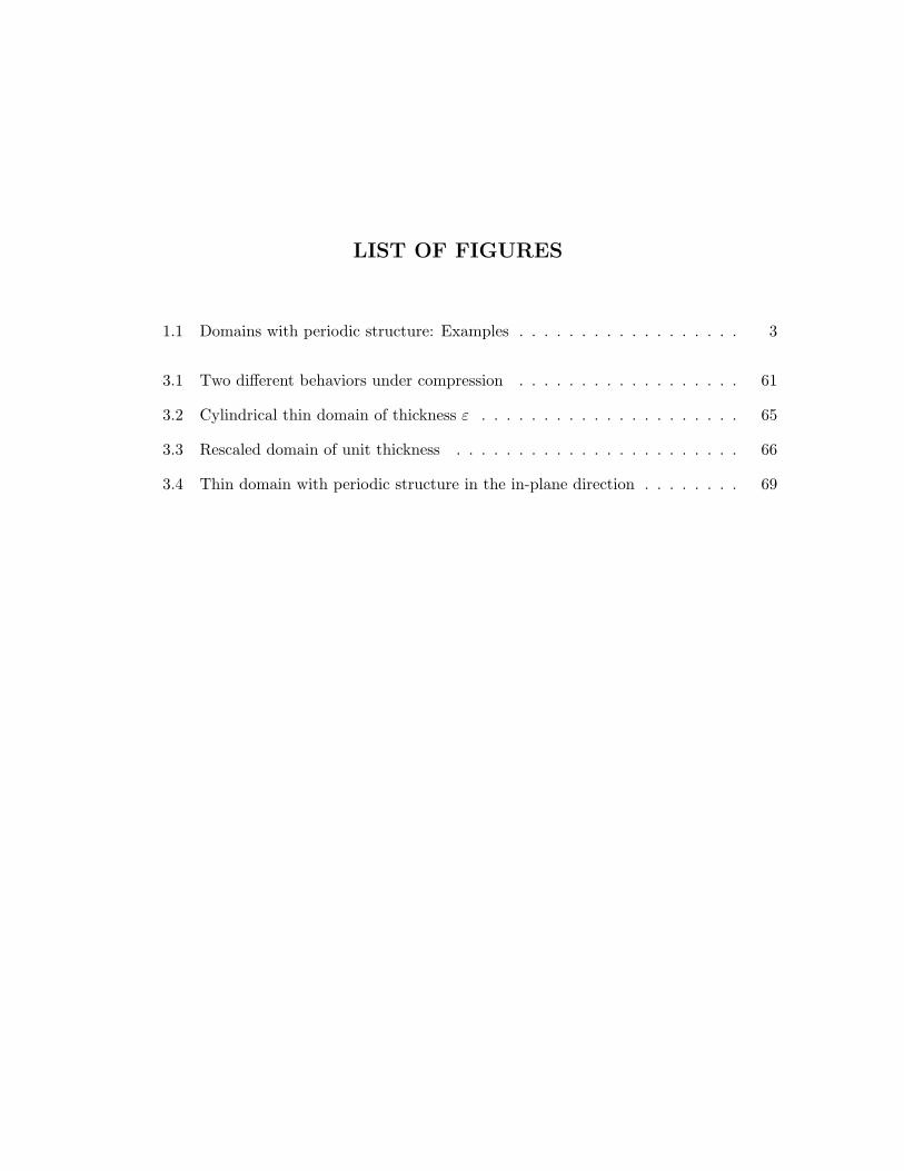
LIST OF FIGURES
1.1 Domains with periodic structure: Examples . . . . . . . . . . . . . . . . . . 3
3.1 Two different behaviors under compression . . . . . . . . . . . . . . . . . . 61
3.2 Cylindrical thin domain of thickness ε . . . . . . . . . . . . . . . . . . . . . 65
3.3 Rescaled domain of unit thickness . . . . . . . . . . . . . . . . . . . . . . . 66
3.4 Thin domain with periodic structure in the in-plane direction . . . . . . . . 69

1. INTRODUCTION
The main objective of this dissertation is to study the effective behavior of elastic (thin)
bodies with multiple scales and periodic microstructure. This study is undertaken from a
variational point of view through an asymptotic analysis based on Γ-convergence arguments.
The asymptotic analysis of media with multiple scale of homogenization is referred to in
the literature as Reiterated Homogenization.
Roughly speaking, the aim of homogenization theory is to describe the behavior of micro-
scopically heterogeneous composite physical structures by means of homogeneous structures
with global characteristics equivalent to the initial ones. In many physical situations the
heterogeneities are very small in comparison with the region in which the structure is to
be studied and the heterogeneities are evenly distributed, so that they can be modelled by
a periodic distribution of period a small parameter. In practice, one is interested in the
global behavior of these structures when the heterogeneities are very, very small. From
the mathematical point of view, we are led to characterizing the asymptotic behavior of
(systems of) ordinary or partial differential equations with oscillating periodic coefficients
of period a small parameter ε, as ε tends to zero.
A well-known model problem in periodic homogenization, used frequently to describe ther-
mal as well as electrical or linear elasticity properties in a periodic composite medium has
as underlying the following linear second-order partial differential equation
−div(
A(x
ε
)
∇uε)
= g on Ω. (1.1)
Here Ω is the (material) domain in RN (N > 1), A is a scalar or tensor-valued function with
periodic coefficients, and uε and g are scalar or vector-valued functions in some appropriate
functional spaces. One wishes to know the asymptotic behavior of the solutions uε as ε→ 0.
1. Introduction 2
They converge, under appropriate hypotheses, to a solution of an “homogenized” differential
equation of the form
−div(Ahom(∇u)) = g on Ω.
Starting with the use of asymptotic expansions methods (see Bensoussan, Lions and Papan-
icolau [14], Jikov, Kozlov and Oleinik [58] and Sanchez-Palencia [72]) adapted to the study
of periodic problems like (1.1), homogenization techniques evolved toward more general sit-
uations through the concepts of G-convergence due to Spagnolo (see [74]), of H-convergence
due to Murat and Tartar (see [68] [67], and [76]), of Γ-convergence due to De Giorgi (see [38]
and [40]), and of two-scale convergence due to Nguetseng (see [61], [69] and [70]), further
developed by Allaire and Briane (see [4] and [5]), and generalized by many other authors.
We refer to the book of Cioranescu and Donato [32] for an introduction to homogenization
and for an overview of different homogenization methods.
From a variational point of view, for instance in the context of elasticity, the theory of
periodic homogenization rests on the study of a family of minimum problems
min
∫
Ωfε(x, u(x),∇u(x)) dx+
∫
Ωug dx : u = ϕ on ∂Ω
, (1.2)
where the functions fε (the elastic density energy) are increasingly oscillating in the first
variable as ε tends to zero, and u (the deformation), g (the density of applied body forces)
and ϕ are scalar or vector-valued functions in some Sobolev space. In the example (1.1)
if A = (Aij) and u is a scalar function, fε(x,∇u) =∑
Aij(xε )∇iu∇ju, where ∇i = ∂/∂xi.
More general minimum problems can be considered but in this Introduction we restrict to
this case for simplicity. The homogenization of the family of minimum problems (1.2) leads
to an “effective homogenized minimum problem” (not depending on ε)
min
∫
Ωfhom(x, u(x),∇u(x)) dx+
∫
Ωug dx : u = ϕ on ∂Ω
(1.3)
such that a sequence of minimizers of (1.2) converges, as ε tends to zero, to a limit u, which
is a minimizer of (1.3). The fundamental property of De Giorgi’s notion of Γ-convergence,
and its main link to the other homogenization techniques, is that, under certain growth and
compactness properties on fε and some regularity on g, it implies a sequence of minimizers
of (1.2) has this convergence property.
Due to the the properties of Γ-convergence (see Theorem 2.5.11 and Propositions 2.5.6 and
2.5.13 below), the convergence of minimizers (or almost minimizers) of (1.2) to minima of

1. Introduction 3
(1.3) can be derived from the Γ-convergence of the family
Iε(u) =
∫
Ωfε(x, u(x),∇u(x)) dx (1.4)
to the homogenized functional
Ihom(u) =
∫
Ωfhom(x, u(x),∇u(x)) dx.
This functional provides the macroscopic, or average description, of the periodic body by
capturing the limiting behavior of the equilibrium states of Iεε. The effective energy
density fhom is to be determined.
In this work we seek to approximate, in a Γ-convergence sense, the behavior of elastic (thin)
bodies whose microstructure is periodic of period ε and ε2 (Figure. 1.1).
ε
ε ε
Fig. 1.1: Domains with periodic structure: Examples
ε
ε
ε2ε
To describe this behavior, let us introduce some notation. We identify Rd×N (resp. Qd×N )
with the set of real (resp. rational)-valued d × N matrices, with d,N > 1. For ξ ∈ R3×2
and z ∈ R3, let (ξ|z) denote the matrix whose first two columns are those of ξ and the last
one is z. Let xα := (x1, x2), with x1, x2 ∈ R and let ∇α = (∇1,∇2). We will consider two
families of energies:
Iε(u) =
∫
Ωf(
x,x
ε,x
ε2,∇u(x)
)
dx
for Ω ⊂ RN , and
Wε(u) :=
∫
ΩW
(
x,x
ε,xαε2,∇αu(x)
∣
∣
∣
1
ε∇3u(x)
)
dx,

1. Introduction 4
for Ω := ω × I, ω ⊂ R2 and I := (−1, 1).
The functional Iε(u) can be interpreted as the energy of a deformation u of an elastic
body whose microstructure is periodic of period ε and ε2. Similarly, as it will be seen
later (Section 3.2), the functional Wε(u) can be interpreted as the rescaled energy of a
deformation u of a cylindrical thin film of thickness ε whose microstructure is periodic of
period ε in the in-plane direction xα, and periodic of period ε2 in all directions. The variable
x is called the macroscopic or slow variable, whereas the variables y = x/ε and z = x/ε2
(respectively z = xα/ε2) are called the microscopic or fast variables. Roughly speaking, the
dependence of the energy on x captures its macroscopic variation while the dependence on
y and z captures its microscopic or local variations. One could generalize the study to a
higher number of scales by iterating the argument.
The overall plan of this dissertation in the ensuing chapters is as follows. Chapter 2 is of
introductory nature. Its objective is to set up the basic notations and background results
that are used later. The aim of Chapter 3 is to present the previous developments in the
asymptotic analysis of this type of problems. This serves as a motivation for our work and
highlights the novelties. Chapter 4 is a collection of two works, obtained in collaboration
with J-F Babadjian [10] and with I. Fonseca [12], respectively. We consider Ω ⊂ RN (N > 1)
open and bounded, 1 < p <∞, and use the notation Γ(Lp(Ω))-limit to refer to the Γ-limit
with respect to the usual metric in Lp(Ω; Rd) with d > 1. We set Q := (0, 1)N and LN
stands for the Lebesgue measure in RN .
Main problem of Chapter 4 (Theorem 4.2.1): Characterize the behavior, as ε tends to zero,
of a family of integral functionals defined on Lp(Ω; Rd) by
Iε(u) :=
∫
Ωf(
x,x
ε,x
ε2,∇u(x)
)
dx if u ∈W 1,p(Ω; Rd),
∞ otherwise,
(1.5)
where the integrand f : Ω × RN × RN × Rd×N → R satisfies:
- f(x, · , · , · ) is continuous for a.e. x ∈ Ω;
- f( · , y, z, ξ) is LN -measurable for all (y, z, ξ) ∈ RN × RN × Rd×N ;
- f(x, · , z, ξ) is Q-periodic for all (z, ξ) ∈ RN ×Rd×N and for a.e. x ∈ Ω; f(x, y, · , ξ) is
Q-periodic for all (y, ξ) ∈ RN × Rd×N and for a.e. x ∈ Ω;
1. Introduction 5
- there exists β > 0 such that for all (y, z, ξ) ∈ RN × RN × Rd×N and for a.e. x ∈ Ω
1
β|ξ|p − β 6 f(x, y, z, ξ) 6 β(1 + |ξ|p).
This kind of asymptotic problems can be seen as a generalization of the Iterated Homoge-
nization Theorem for linear integrands, proved by Bensoussan, Lions and Papanicolau [14],
in which the homogenized operator is derived by a formal two-scale asymptotic expansion
method. In the Γ-convergence setting it is customary to assume that
|f(x, y, z, ξ) − f(x′, y′, z, ξ)| 6 ω(|x− x′| + |y − y′|)[
b(z) + f(x, y, z, ξ)]
, (1.6)
for some b ∈ L1loc(R
N ) and some continuous positive real function ω with ω(0) = 0 (see
Braides and Defranceschi [19], Braides and Lukkassen [21] and Lukkassen [60]). As remarked
by Allaire (Section 5 in [4]), the natural regularity on f for the integral (1.5) to be well
defined is not clear. The measurability of the function x 7→ f(x, x/ε, x/ε2, ξ), for fixed ξ, is
assured whenever f is continuous in its second and third variables. The originality of this
work is that we do not require any strong uniform continuity hypotheses on f with respect
to the first and second variables. In particular, we will recover the results of Fonseca and
Zappale in [51], where the authors were also able to weaken hypothesis (1.6) in the convex
case when f = f(y, z, ξ), but by using multiscale arguments that however cannot be adapted
to the nonconvex setting.
As previous results show, the natural candidate for the Γ(Lp(Ω))-limit functional of the fam-
ily Iεε is the functional obtained by iterating twice the homogenization formula derived
for functionals of the type∫
Ωf(
x,x
ε,∇u(x)
)
dx.
Therefore, we expect that
Ihom(u) :=
∫
Ωfhom(x,∇u(x)) dx if u ∈W 1,p(Ω; Rd),
∞ otherwise,
(1.7)
where fhom is defined, for all ξ ∈ Rd×N and for a.e. x ∈ Ω, by
fhom(x, ξ) := limT→∞
infφ
1
TN
∫
(0,T )N
fhom(x, y, ξ + ∇φ(y)) dy : φ ∈W 1,p0
(
(0, T )N ; Rd)
,

1. Introduction 6
and where, for all (y, ξ) ∈ RN × Rd×N and for a.e. x ∈ Ω,
fhom(x, y, ξ) := limT→∞
infφ
1
TN
∫
(0,T )N
f(x, y, z, ξ + ∇φ(z)) dz : φ ∈W 1,p0
(
(0, T )N ; Rd)
.
The analysis we do calls for a new look into the following auxiliary problem.
Auxiliary problem (Theorem 4.1.1): Study the asymptotic behavior of the functional Iε :
Lp(Ω; Rd) → R, where R := R ∪ ∞, given by
Iε(u) :=
∫
Ωf(
x,x
ε,∇u(x)
)
dx if u ∈W 1,p(Ω; Rd),
∞ otherwise.
(1.8)
This analysis undertaken in Section 4.1 by means of two-scale convergence arguments allows
us to weaken the hypotheses considered in previous works (see Braides [15], Braides and
Defranceschi [19] and Braides and Lukkassen [21]), and consequently derive (1.7).
Chapter 5 collects parts of two joint works with J-F Babadjian [9, 10]. Here we study the
asymptotic behavior of cylindrical heterogeneous thin domains whose microscopic hetero-
geneities vary periodically. More precisely, given ω ⊂ R2 open and bounded, we consider
thin microstructures of the form Ωε := ω× (−ε, ε), whose heterogeneities are periodic of pe-
riod ε in the in-plane direction and of period ε2 in all directions. Two simultaneous features
occur in this case: a reiterated homogenization and a dimension reduction phenomena. As
is usual, in order to study this asymptotic problem we rescale the thin body into a reference
domain of unit thickness Ω := ω × (−1, 1) (see e.g. Acerbi, Buttazzo and Percivale [2], Le
Dret and Raoult [55]), and we study the rescaled family of functionals defined on Ω, whose
dependence on ε turns out to be explicit in the transverse derivative.
Main problem of Chapter 5 (Theorem 5.2.4): Characterize the behavior as ε tends to zero
of the family of rescaled functionals defined on Lp(Ω; Rd) by
Wε(u) :=
∫
ΩW
(
x,x
ε,xαε2,∇αu(x)
∣
∣
∣
1
ε∇3u(x)
)
dx if u ∈W 1,p(Ω; R3),
∞ otherwise,
(1.9)
where W : Ω × R3 × R2 × R3×3 → R satisfies:

1. Introduction 7
- W (x, · , · , · ) is continuous for a.e. x ∈ Ω;
- W ( · , · , · , ξ) is L3 ⊗ L3 ⊗ L2-measurable for all ξ ∈ R3×3;
- yα 7→ W (x, yα, y3, zα, ξ) is Q′-periodic for all (zα, y3, ξ) ∈ R3 × R3×3 and for a.e. x ∈Ω, where Q′ := (0, 1)2;
- (zα, y3) 7→W (x, yα, y3, zα, ξ) is Q -periodic for all (yα, ξ) ∈ R2×R3×3 and for a.e. x ∈Ω, where Q := (0, 1)3;
− there exists β > 0 such that for all (y, zα, ξ) ∈ R3 × R2 × R3×3 and for a.e. x ∈ Ω
1
β|ξ|p − β 6 W (x, y, zα, ξ) 6 β(1 + |ξ|p).
We identify W 1,p(ω; R3) with the set of functions u ∈W 1,p(Ω; R3) such that D3u(x) = 0 for
a.e. x ∈ Ω. Under the above hypotheses, the Γ(Lp(Ω))-limit of the family Wεε is given
by the functional
Whom(u) :=
2
∫
ωW hom(xα,∇αu(xα)) dxα if u ∈W 1,p(ω; R3),
∞ otherwise,
where W hom is defined, for all ξ ∈ R3×2 and for a.e. xα ∈ ω, by
W hom(xα, ξ) := limT→∞
infφ
1
2T 2
∫
(0,T )2×IWhom(xα, y3, yα, ξ + ∇αφ(y)|∇3φ(y)) dy :
φ ∈W 1,p((0, T )2 × I; R3), φ = 0 on ∂(0, T )2 × I
(1.10)
and where, for all (yα, ξ) ∈ R2 × R3×3 and for a.e. x ∈ Ω,
Whom(x, yα, ξ) := limT→∞
infφ
1
T 3
∫
(0,T )3W (x, yα, z3, zα, ξ + ∇φ(z)) dz :
φ ∈W 1,p0 ((0, T )3; R3)
.
Our main contribution is that we are able to homogenize this material in the reducing
direction. As far as we know, there have not been previous results in this direction (see
Braides, Fonseca and Francfort [20] and Shu [75]). Let us outline the idea for the derivation
of the formula (1.10). In a first step, since the volume of Ωε is of order ε and ε2 ≪ ε, we

1. Introduction 8
can think of ε as being a fixed parameter and let ε2 tend to zero. At this point, dimension
reduction is not occurring, and (1.9) can be seen as a single one-scale homogenization
problem, as in (1.5). This leads to the stored energy density Whom(x, yα, ξ). In a second
step, Whom(x, yα, ξ) is used as the integrand for the following reduction dimension problem.
Auxiliary problem (Theorem 5.1.1): Characterize the asymptotic behavior of a family of
functionals Iε : Lp(Ω; R3) → R given by
Iε(u) :=
∫
ΩW
(
x,xαε,∇αu(x)
∣
∣
∣
1
ε∇3u(x)
)
dx if u ∈W 1,p(Ω; R3),
∞ otherwise.
This problem will be studied in Section 5.1. Two features differentiate our approach from
what is available in most of the literature on the subject (see Braides, Fonseca and Francfort
[20] and Shu [75]; see also Chapter 3). The first feature is the use of a two-scale convergence
argument as in problem (1.8). The second feature is a decoupling argument, motivated by
the work in Babadjian and Francfort [11], to take into account the different nature of the
variables that appear in the structure of the limit functional.
We note that if Ω is assumed to be Lipschitz, as p > 1, the Γ-limit of the previous functionals
for u ∈ W 1,p(Ω; Rd) would be the same if the weak W 1,p-topology had been considered in
place of the strong Lp-topology. For p = 1 our argument fails to characterize this Γ-limit
for u ∈ W 1,1(Ω; Rd), either with the strong L1-topology or with the weak W 1,1-topology,
since sequences whose gradients are bounded in L1 are not necessarily relatively compact
in W 1,1(Ω; Rd). They are relatively compact only in the space of functions of bounded
variation.
We finally remark that, from the applications point of view, it would be interesting to
prove similar results to the ones addressed in Chapters 4 and 5 for integrands that are only
measurable with respect to (some of) the oscillating variables. This is what is relevant in
the case of mixtures. In Chapter 6 we conclude with some generalizations in this direction
and we address some open problems for future research.
Part I
PRELIMINARIES AND PREVIOUS RESULTS


2. PRELIMINARIES
The purpose of this introductory chapter is to give a survey of the concepts and results that
are used throughout this dissertation. Almost all these results are stated without proofs as
they can be readily found in the references given below.
2.1 A short review of Measure Theory
In this section we recall well known results in Measure Theory (see e.g Ambrosio, Fusco and
Pallara [7], Evans and Gariepy [46] and Fonseca and Leoni [47], as well as the bibliography
therein; see also Brezis [29] and Dugundji [44] for a reference on functional analysis and
topological notions).
2.1.1 Measures and integration
A measurable space is a pair (X,M) where X is a nonempty set and M is a σ-algebra in
X. A set E ⊂ X is said to be measurable if E ∈ M. If X is a topological space and if not
otherwise said, then M is taken to be the Borel σ-algebra in X, that we denote by B(X),
i.e. the smallest σ-algebra that contains all open subsets of X.
Definition 2.1.1. (Measure) A measure on (X,M) is a set function µ : M → [0,∞] such
that µ(∅) = 0 and µ is σ-additive, i.e.
µ(
∞⋃
n=0
En
)
=∞∑
n=0
µ(En)
for any sequence Enn of pairwise disjoint elements of M.
The triple (X,M, µ) is called a measure space; it is said to be σ-finite if X is the union of
an increasing sequence of sets with finite µ-measure, and it is said to be finite if µ(X) <∞.

2. Preliminaries 12
Definition 2.1.2. (Borel measure) Let X be a topological space and let (X,M, µ) be a
measure space. The measure µ is said to be Borel if B(X) ⊆ M.
Remark 2.1.3. Any measure µ on (X,M) is monotone with respect to set inclusion and
continuous along monotone sequences, that is, if Enn is an increasing sequence of sets
(respectively a decreasing sequence of sets with µ(E1) finite), then
µ(
∞⋃
n=1
En
)
= limn→∞
µ(En), resp. µ(
∞⋂
n=1
En
)
= limn→∞
µ(En).
Definition 2.1.4. Let (X,M, µ) be a measure space.
i) A set N ⊂ X is said to be µ-negligible if there exists E ∈ M such that N ⊂ E and
µ(E) = 0.
ii) A property P (x), depending on the point x ∈ X, is said to hold µ-a.e. (or simply
a.e. ) in X if the set where P fails is a µ-negligible set.
Proposition 2.1.5. Let (X,M, µ) be a measure space and let Mµ be the collection of all
the subsets of X of the form F = E ∪N , with E ∈ M and N µ-negligible. Then Mµ is a
σ-algebra and it is called the µ-completion of M.
Definition 2.1.6. (µ-measurable set) Let (X,M, µ) be a measure space. A set E ⊂ X is
said to be µ-measurable if E ∈ Mµ.
Given (X,M, µ) a measure space the measure µ extends to Mµ by setting, for F as above,
µ(F ) = µ(E), and µ is said to be complete if M = Mµ. Throughout this work any Borel
measure is tacitly understood to be extended to its completion.
We denote by LN the usual Lebesgue measure in RN as well as its restriction to B(RN ). The
set LN stands for the σ-algebra of all Lebesgue measurable sets (that is L
N = B(RN )LN ).
Given E ∈ LN , we will write indifferently LN (E) or |E|.
Definition 2.1.7. Let (X,M) and Y be, respectively, a measurable and a topological
space. Let u : X → Y .
i) (Measurable function) The function u is said to be M-measurable, or simply measur-
able, if u−1(B) ∈ M for every open set B ⊂ Y.
ii) (Borel function) Assuming that X is also a topological space, the function u is said
to be Borel if u−1(B) ∈ B(X) for every open set B ⊂ Y.

2. Preliminaries 13
Definition 2.1.8. (µ- measurable function) Let (X,M, µ) and Y be, respectively, a mea-
sure and topological space. A function u : X → Y is said to be µ-measurable if it is
Mµ-measurable.
The following theorem provides conditions guaranteeing the existence of a measurable se-
lection of a given multifunction. It can be found in Castaing and Valadier [30] (Theorem
III.30) and it is important for the analysis undertaken in Subsection 4.2.4 below.
Theorem 2.1.9. Let (X,M, µ) be a finite complete measure space, and let Y be a complete
and separable metric space. Let F : X → C ⊂ Y : C 6= ∅ and C is a closed set be a
multifunction such that (x, y) ∈ X × Y : y ∈ F (x) ∈ M ⊗ B(Y ).1 Then there exists a
sequence of measurable functions un : X → Y such that
F (x) = un(x) : n ∈ N
for µ a.e. x ∈ X.
Let (X,M, µ) be a measure space and let us denote by Lp(X,µ), with 1 6 p 6 ∞ , the usual
Lebesgue spaces, that is the set (of the equivalence classes) of all µ-measurable functions
u : X → R such that the (Lebesgue) integral
||u||Lp(X,µ) :=
(∫
X|u|p dµ
)1/p
<∞
for p <∞, or
||u||L∞(X,µ) := infC ∈ [0,∞] : |u(x)| 6 C for µ-a.e. x ∈ X <∞.2
We abbreviate Lp(X,µ) by Lp(X) when this will cause no confusion (e.g. when µ is the
Lebesgue measure in RN ). Is is well known that Lp(X,µ) is a Banach space with the norm
|| · ||Lp(X,µ) for 1 6 p 6 ∞ (Hilbert when p = 2); it is a reflexive space for 1 < p < ∞, and
in this case its dual space is (identified with) Lq(X) with q = p/(p − 1). If (X,M, µ) is
σ-finite then L∞(X,µ) is the dual space of L1(X,µ); if, in addition, X is separable3 then
Lp(X,µ) is separable for 1 6 p <∞.
1 The set M⊗B(Y ) denotes the usual product σ-algebra of M and B(Y ).2 ||u||L∞(X,µ) is sometimes called the essential supremum of u and written ||u||L∞(X,µ) = ess sup
x∈X
|u(x)|;
usual convention: inf∅ = ∞.3 We recall that a measurable space (X,M) is said to be separable if there exists a sequence Enn ⊂ M
such that the smallest σ-algebra that contains all the sets En is M. If X is a metric space and M is a Borel
σ-algebra, then (X,B(X)) is a separable space.
2. Preliminaries 14
Lemma 2.1.10. (Chebyshev inequality) Let (X,M, µ) be a measure space. If u ∈ Lp(X;µ),
with 1 6 p <∞, then for any t > 0
µ(x ∈ X : |u(x)| > t) 61
tp
∫
X|u|p dµ.
We assume that the reader is familiar with the properties of integrals, measurable functions
and Lp-spaces. For the sake of completeness we state here the fundamental convergence
results in the theory of integration on abstract measure spaces.
Theorem 2.1.11. (Levi’s Theorem or Monotone Convergence Theorem) Let (X,M, µ) be
a measure space, and let un : X → R be an increasing sequence of µ-measurable functions.
Assume that un > v for any n ∈ N, with v ∈ L1(X,µ), then
limn→∞
∫
Xun dµ =
∫
Xlimn→∞
un dµ.
Lemma 2.1.12. (Fatou’s Lemma) Let (X,M, µ) be a measure space and let un : X → R
be a sequence of µ-measurable functions.
i) If there exists v ∈ L1(X,µ) such that un > v for any n ∈ N, then∫
Xlim infn→∞
un dµ 6 lim infn→∞
∫
Xun dµ.
ii) If there exists v ∈ L1(X,µ) such that un 6 v for any n ∈ N, then∫
Xlim supn→∞
un dµ > lim supn→∞
∫
Xun dµ.
As a consequence we get the following result.
Corollary 2.1.13. Let (X,M, µ) be a measure space and let un ⊂ Lp(X,µ) with 1 6
p < ∞, be such that un → u µ-a.e. as n → ∞, for some function u ∈ Lp(X,µ). Then
||un − u||Lp(X,µ) → 0 if and only if ||un||Lp(X,µ) → ||u||Lp(X,µ).
Theorem 2.1.14. (Dominated Convergence Theorem) Let u, un : X → R be µ-measurable
functions, and assume that un → u µ-a.e. as n→ ∞. If∫
Xsupn∈N
|un| dµ <∞
then
limn→∞
∫
Xun dµ =
∫
Xu dµ.
2. Preliminaries 15
The following variant of the Dominated Convergence Theorem can be found in Evans and
Gariepy [46] and it will be of use in the sequel.
Proposition 2.1.15. Let v, vn ∈ L1(X,µ) and let u, un be µ-measurable, for n ∈ N.
Suppose that |un| 6 vn for all n ∈ N, and that un and vn converge µ-a.e. to u and v,
respectively. If in addition
limn→∞
∫
Xvn dµ =
∫
Xv dµ,
then
limn→∞
∫
X|un − u|dµ = 0.
Theorem 2.1.16. (Fubini-Tonelli Theorem) Let (X1,M1, µ1) and (X2,M2, µ2) be two σ-
finite measure spaces. Then, there is a unique positive σ-finite measure µ on (X1×X2,M1⊗M2) such that
µ(E1 × E2) = µ1(E1)µ2(E2)
for all E1 ∈ M1 and E2 ∈ M2.
i) (Tonelli) In addition, for any measurable function u : X1 ×X2 → [0,∞] we have that
x→∫
X2
u(x, y)dµ2(y) and y →∫
X1
u(x, y)dµ1(x)
are M1-measurable and M2-measurable respectively, and∫
X1×X2
u dµ =
∫
X1
(∫
X2
u(x, y)dµ2(y)
)
dµ1(x) (2.1)
=
∫
X2
(∫
X1
u(x, y)dµ1(x)
)
dµ2(y).
ii) (Fubini) If u ∈ L1(X1 ×X2;µ), then u(x, ·) ∈ L1(X2, µ2) for µ1-a.e. x ∈ X1, u(·, y) ∈L1(X1, µ1) for µ2-a.e. y ∈ X2, the a.e. defined functions
x→∫
X2
u(x, y)dµ2(y) and y →∫
X1
u(x, y)dµ1(y)
are in L1(X1, µ1) and L1(X2, µ2), respectively, and equality (2.1) holds.
We present here another version of Fubini-Tonelli’s Theorem which deals with complete
measures and is relevant to Lebesgue integration on RN .

2. Preliminaries 16
Theorem 2.1.17. Suppose that (X1,M1, µ1) and (X2,M2, µ2) are two complete and σ-
finite measure spaces. If u : X1 × X2 → [0,∞] is µ-measurable (where µ is the measure
given by theorem 2.1.16)4, then the functions
x→∫
X2
u(x, y)dµ2(y) and y →∫
X1
u(x, y)dµ1(y)
are respectively µ1-measurable and µ2-measurable and
∫
X1×X2
u dµ =
∫
X1
(∫
X2
u(x, y)dµ2(y)
)
dµ1(x)
=
∫
X2
(∫
X1
u(x, y)dµ1(x)
)
dµ2(y).
2.1.2 Radon measures and Vitali’s Covering Theorem
Definition 2.1.18. (Radon Measure on (X,M)) Let X be a topological space. A Radon
measure on a measurable space (X,M) is a Borel measure, finite on compact sets, and such
that for every open set E ⊂ X
µ(E) = supµ(K) : K ⊂ E, K compact (inner-regularity),
and for every set E ∈ M
µ(E) = supµ(A) : E ⊂ A, A open (outer-regularity).
Remark 2.1.19. If X is a locally compact Hausdorff space the following two properties hold.5
i) (see Theorem 2.7 in Rudin [71]) Let E,K ⊂ X be an open and compact set, re-
spectively, with K ⊂ E. Then there is an open set A with compact closure such
that
K ⊂ A ⊂ A ⊂ E.
4 By Definition 2.1.6 this means measurable with respect to the completion σ-algebra of M1 ⊗M2; if µ is
a Borel measure then it is understood to be extended to (M1 ⊗M2)µ. In the case of the Lebesgue measure
B(RN ) = B(R)N-times⊗ · · · ⊗ B(R).
5 A topological space X is said to be Hausdorff if given two distinct points x and y, there are disjoint
open sets E1 and E2 such that x ∈ E1 and y ∈ E2; X is said to be locally compact if for each x ∈ X there
is an open set E containing x such that E is compact. Metric spaces are Hausdorff spaces and RN with the
usual metric is Hausdorff and locally compact.

2. Preliminaries 17
ii) Let µ be a Radon measure on X and let E be an open set of X. Then
µ(E) = supµ(K) : K ⊂ E, K compact = supµ(A) : A ⊂⊂ E,A open,
where A ⊂⊂ E means that A is a compact set with A ⊂ E.
Given a topological space X we denote by A(X) the family of all its open subsets. The
following lemma provides sufficient conditions for a set function Π : A(X) → [0,∞) to
be the restriction of a Radon measure on A(X). It is close in spirit to De Giorgi-Letta’s
criterion (see [39]) and it is of importance to apply the Direct Method of Γ-convergence (see
Chapters 4 and 5 below) as well as for the use of relaxation methods that strongly rely on
the structure of Radon measures.
Lemma 2.1.20. (see Fonseca and Maly [48]; also Fonseca and Leoni [47]) Let X be a locally
compact Hausdorff space, let Π : A(X) → [0,∞), and let µ be a finite Radon measure µ on
X satisfying
i) (nested-subadditivity) Π(D) ≤ Π(D\B) + Π(C) for all B,C,D ∈ A(X) with B ⊂⊂C ⊂ D;
ii) Given D ∈ A(X), for all ǫ > 0 there exists Dε ∈ A(X) such that Dε ⊂⊂ D and
Π(D\Dε) ≤ ε;
iii) Π(X) ≥ µ(X);
iv) Π(D) ≤ µ(D) for all D ∈ A(X).
Then Π = µ|A(X).
Proof. Fix D ∈ A(X). We start by proving that the inequality Π(D) 6 µ(D) holds. Let
ε > 0 and by condition ii) choose Dε ∈ A(X) such that Dε is a compact set, Dε ⊂ D and
Π(D\Dε) ≤ ε. As X is a locally compact Hausdorff space, we can find Cε ∈ A(X) such
that Dε ⊂ Cε ⊂ Cε ⊂ D (see Remark 2.1.19).
By hypotheses i), ii) and iv) we have
Π(D) 6 Π(D \Dε) + Π(Cε) 6 ε+ µ(Cε) 6 ε+ µ(D),

2. Preliminaries 18
DDεCε
and then letting ε→ 0 it follows that
Π(D) 6 µ(D).
To prove the reverse inequality, using the inner regularity property of the measure µ (see
Remark 2.1.19), for every ε > 0 we may find B ∈ A(X) with B ⊂⊂ D and such that
µ(D) 6 ε+ µ(B).
Therefore
µ(D) 6 ε+ µ(X) − µ(X \B)
and, consequently, by iii) and the previous step
µ(D) 6 ε+ Π(X) − Π(X \B).
Hence by i) we have
µ(D) 6 ε+ µ(D)
and therefore letting ε→ 0 we get µ(D) 6 Π(D).
Given a ∈ RN and δ > 0 we denote by B(a, δ) := x ∈ RN : |x− a| < δ.
Theorem 2.1.21. (Vitali’s Covering Theorem) (see Braides and Defranceschi [19]) Let
Ω ⊂ RN be a bounded open set with N > 1, and let F be a family of closed subsets of Ω. If
there exists a positive number M > 1 such that for each F ∈ F , B(x, δ) ⊆ F ⊆ B(x,Mδ)
for some x ∈ Ω and δ > 0, and if
infdiamF : x ∈ F, F ⊂ F = 0
for a.e. x ∈ Ω, then there exists a disjoint countable subfamily Fjj of F such that∣
∣
∣Ω \⋃
j
Fj
∣
∣
∣ = 0.

2. Preliminaries 19
2.1.3 Decomposition and differentiation of measures
Definition 2.1.22. Let (X,M, µ) and (X,M, ν) be two measure spaces. The measure ν
is said to be absolutely continuous with respect to µ, and we write ν << µ, if for every
E ∈ M the following implication holds:
µ(E) = 0 ⇒ ν(E) = 0.
The measures µ and ν are said to be mutually singular, and we write ν ⊥ µ, if there exists
E ∈ M such that µ(E) = 0 and ν(X \ E) = 0.
Theorem 2.1.23. (Lebesgue-Radon-Nikodym Theorem) Let (X,M, µ) and (X,M, ν) be
two σ-finite measure spaces. Then there exists a unique pair of measures νa and νs such
that νa << µ, νs ⊥ µ and ν = νa + νs. Moreover, there is a unique measurable function
u : X → [0,∞] such that for all E ∈ M
νa(E) =
∫
Eu dµ.
The decomposition ν = νa + νs, where νa << µ and νs ⊥ µ, is called the Lebesgue decom-
position of ν with respect to µ. In the case where ν << µ, Theorem 2.1.23 says that
ν(E) =
∫
Eu dµ
for all E ∈ M. This result is known as the Radon-Nikodym Theorem, and u is called the
Radon-Nikodym derivative of ν with respect to µ, u = dν/dµ.
Theorem 2.1.24. (General version of the Besicovitch derivation Theorem)(see Proposition
2.2 in Ambrosio and Dal Maso [6]) Let µ and ν be two Radon measures on RN and let
ν = νa + νs be the Lebesgue decomposition of ν with respect to µ (dνa = udµ). There exists
a Borel set E ⊂ RN , with µ(E) = 0, such that, for every x ∈ RN \ E and C ⊂ RN open
bounded convex set containing the origin, the limit
limδ↓0
ν(x+ δC)
µ(x+ δC)
exists, is finite, and coincides with u(x).
Let X be a topological space and let µ be a measure on X. A function u is said to be in
L1loc(X,µ) if u ∈ L1(E, µ) whenever E ⊂⊂ X. Theorem 2.1.24 implies the following result.
2. Preliminaries 20
Proposition 2.1.25. (Lebesgue Differentiation Theorem) Let µ be a Radon measure on
RN and let u ∈ L1loc(R
N , µ). Then for a.e. x ∈ RN
limδ↓0
1
µ(B(x, δ))
∫
B(x,δ)|u(y) − u(x)| dµ(y) = 0, (2.2)
and in particular
u(x) = limδ↓0
1
µ(B(x, δ))
∫
B(x,δ)u(y) dµ(y).
Definition 2.1.26. Any point x where (2.2) holds is called a Lebesgue point of u.
Theorem 2.1.27. (see Theorem 2.8 in Fonseca and Muller [49]) Let µ be a Radon measure
on RN and u ∈ L1loc(R
n, µ). Then there exists a Borel set E ⊂ RN , with µ(E) = 0, such
that for every x ∈ RN \ E
limδ↓0
1
µ(x+ δC)
∫
x+δC|u(y) − u(x)| dµ(y) = 0, (2.3)
for every C ⊂ RN open bounded convex set containing the origin.
Definition 2.1.28. (Signed measure) A signed measure on a measurable space (X,M) is
a set function µ : M → [−∞,∞] such that µ(∅) = 0, µ takes at most one of the values ∞or −∞, and for any family Enn of pairwise disjoint elements of M
µ(
∞⋃
n=0
En
)
=∞∑
n=0
µ(En).6
In particular a measure is a signed measure.
Definition 2.1.29. (Total variation of a signed measure) Let (X,M) be a measurable
space and let µ : M → [−∞,∞] be a signed-measure. Its total variation |µ| : M → [0,∞]
is defined by
|µ|(E) := sup
∞∑
n=0
|µ(En)| : En ∈ B(M) pairwise disjoint, E =∞⋃
n=0
En
.
If µ is a positive measure then µ = |µ|, and if µ is a signed-measure then |µ| is a measure.
The signed measure µ is said to be σ-finite if |µ| is a σ-finite measure on X; µ is said to be
a (signed) Radon measure if its total variation |µ| is a Radon measure. Finally, given two
signed measures µ and τ on a measurable space (X,M), µ is absolutely continuous with
respect to τ (respectively mutually singular) if |µ| << |τ | (respectively |µ| ⊥ |τ |), and an
analog of the Lebesgue-Radon-Nikodym Theorem holds for signed-measures.
6 The absolutely convergence of this series is understood.

2. Preliminaries 21
2.1.4 Weak⋆ convergence of measures
Let X be a locally compact Hausdorff space, and let Cc(X) denote the set of continuous
functions with compact support on X. We denote by C0(X) the completion of Cc(X) with
respect to the supremum norm.7 By the Riesz-Representation Theorem the dual of the
Banach space C0(X) is the space of finite (signed) Radon measures µ : B(RN ) → R. This
characterization leads to the following notion of convergence of a sequence of finite (signed)
Radon measures.
Definition 2.1.30. (Weak⋆ convergence of measures) Let µnn be a sequence of finite
(signed) Radon measures on X. This sequence is said to weak⋆ converge to a finite (signed)
Radon measure µ on X, and we write µn⋆ µ, if for all φ ∈ C0(X)
limn→∞
∫
Xφdµn =
∫
Xφdµ.
Proposition 2.1.31. (Weak⋆ compactness property) Let X be a σ-compact metric space.8
Then every sequence µnn of finite (signed) Radon measures on X with supn∈N
|µn|(X) <∞has a weak⋆ converging subsequence.
Proposition 2.1.32. Let X be a locally compact Hausdorff space and let µnn be a se-
quence of finite (signed) Radon measures on X such that µn⋆ µ. Then
i) if K ⊂ X is compact
µ(K) ≥ lim supn→∞
µn(K);
ii) if A ⊂ X is open
µ(A) ≤ lim infn→∞
µn(A);
iii) if A ⊂⊂ X is open and µ(∂A) = 0
µ(A) = limn→∞
µn(A).
7 The support of u is by definition supp (u) := x ∈ X : u(x) 6= 0; the function u is said to have compact
support in X if supp (u) ⊂⊂ X.8 A metric space is said to be σ-compact if it is the union of a countable collection of compact subsets;
for instance RN is a σ-compact metric space.

2. Preliminaries 22
2.2 Sobolev spaces
The aim of this section is to give the main properties needed throughout the text on weak
derivatives and Sobolev spaces. We refer to the books of Adams [3], Brezis [29], Evans and
Gariepy [46], Fonseca and Leoni [47], Giusti [57], and Ziemer [77] for a detailed analysis on
this topic.
2.2.1 Definition and main properties
Let Ω be an open subset of RN with N > 1, and let 1 6 p 6 ∞. In the sequel W 1,p(Ω)
(respectively W 1,ploc (Ω)) stands for the usual Sobolev space, that is the space of functions
u ∈ Lp(Ω) (respectively Lploc(Ω)) with weak derivatives of order one in Lp(Ω) (respectively
Lploc(Ω)).9 For any u ∈W 1,p(Ω) we set ∇u := (∇1u, ...,∇Nu). The space W 1,p0 (Ω) stands for
the closure of C∞0 (Ω) in W 1,p(Ω) for 1 < p <∞. W 1,∞
0 (Ω) denotes the closure of C∞0 (Ω) in
the weak⋆ topology of W 1,∞(Ω). It is well known that W 1,p(Ω) is a Banach space (Hilbert
for p = 2) when endowed with the norm
||u||W 1,p(Ω) :=
(
||u||pLp(Ω) +N∑
i=1
||∇iu||pLp(Ω)
)1/p
for 1 6 p <∞; for p = ∞ the norm is given by
||u||W 1,∞(Ω) := ||u||L∞(Ω) +N∑
i=1
||∇iu||L∞(Ω).10
Since for 1 < p < ∞ the space W 1,p(Ω) is reflexive, for each bounded sequence unn ⊂W 1,p(Ω), with 1 < p < ∞, there exists a subsequence unk
k ⊂ W 1,p(Ω) and u ∈ W 1,p(Ω)
such that unk u in W 1,p(Ω) (see Theorem III.27 in Brezis [29]). For 1 6 p < ∞ the
space W 1,p(Ω) is separable. Finally we remark that the W 1,p(Ω)-weak limit of a sequence
in W 1,p0 (Ω) still belongs to W 1,p
0 (Ω) since a convex subset of a Banach space is closed with
respect to the weak topology if and only if it is closed with respect to the strong topology.
9 For any i ∈ 1, ..., d we set ∇i := ∂/∂xi. Given u, v ∈ Lploc(Ω) we recall that v is said to be the
ith-derivative of u and we write ∇iu = v, provided∫
Ω
u∇iϕ dx = −
∫
Ω
vϕ dx
for all functions ϕ ∈ C∞c (Ω).
10 ||u||W1,p(Ω) ≡ ||u||Lp(Ω) + ||∇u||Lp(Ω).
2. Preliminaries 23
For d > 1 we denote by
Lp(Ω; Rd) :=
u : Ω → Rd : ui ∈ Lp(Ω) for all i ∈ 1, ..., d
;
W 1,p(Ω; Rd) :=
u ∈ Lp(Ω; Rd) : ∇ju ∈ Lp(Ω; Rd) for j = 1, ..., N
,
where ∇ju := (∇ju1, ...,∇jud). If u ∈W 1,p(Ω; Rd) we write ∇u := (∇1u|...|∇Nu).
The following result gives a sufficient condition for a function to belong to W 1,p(Ω). It is a
straightforward consequence of the definition of the space and of the properties above.
Proposition 2.2.1. Let Ω ⊂ RN be open, and let unn be a sequence in W 1,p(Ω) converg-
ing in Lp(Ω) to some function u. Then
i) if 1 6 p 6 ∞ and there exists a function g ∈ Lp(Ω; RN ) such that ∇un → g in
Lp(Ω; RN ), then u ∈W 1,p(Ω) and g = ∇u;
ii) if 1 < p 6 ∞ and the sequence ∇unn is bounded in Lp(Ω; RN ) then u ∈ W 1,p(Ω)
and ∇un ∇u in Lp(Ω; RN ) (weak⋆ if p = ∞).11
2.2.2 Extension, approximation and traces
Theorem 2.2.2. (Extension Theorem) Let Ω be an open bounded subset of RN with Lip-
schitz boundary and let 1 6 p 6 ∞. Let Ω be any open set such that Ω ⊂⊂ Ω. Then there
exist a bounded linear (extension) operator
E : W 1,p(Ω) →W 1,p(RN )
such that Eu = u in Ω and supp(Eu) ⊂ Ω for all u ∈W 1,p(Ω).
Theorem 2.2.3. (Approximation by smooth functions) Let Ω be an open subset of RN and
let 1 6 p <∞. Then
i) (Meyers-Serrin) C∞(Ω) ∩W 1,p(Ω) is dense in W 1,p(Ω);
ii) if, in addition, Ω is a bounded Lipschitz set, then the restriction to Ω of functions in
C∞c (RN ) is dense in W 1,p(Ω).
11 If p = 1 the function u is in BV (Ω), the space of functions with bounded variation, but not necessarily
in W 1,1(Ω).

2. Preliminaries 24
Next we recall a Trace Theorem that makes it possible to assign “boundary values” along
∂Ω to a function u ∈W 1,p(Ω).
Theorem 2.2.4. (Trace Theorem) Let Ω ⊂ RN be a bounded set with Lipschitz boundary,
and let 1 6 p < ∞. Then there exists a bounded linear operator T : W 1,p(Ω) → Lp(∂Ω)
such that
i) Tu = u⌊∂Ω if u ∈ C(Ω);
ii) ||Tu||Lp(∂Ω) 6 C||u||W 1,p(Ω) for each u ∈W 1,p(Ω), for some constant C = C(N, p,Ω).
Moreover Ker(T ) = W 1,p0 (Ω).
2.2.3 Compactness and Poincare inequalities
Theorem 2.2.5. (Sobolev-Rellich-Kondrachov Theorem) Let Ω be an open bounded set in
RN with Lipschitz boundary and let 1 6 p <∞. Then
i) for 1 6 p < N and 1 6 q < p⋆ = NpN−p
W 1,p(Ω) ⊂ Lq(Ω),
and the imbedding is compact;12
ii) if p = N then for every 1 6 q <∞
W 1,p(Ω) ⊂ Lq(Ω),
and the imbedding is compact;
iii) if p > N then
W 1,p(Ω) ⊂ C(Ω),
and the imbedding is compact.
Remark 2.2.6. Under hypotheses of Theorem 2.2.5:12 Recall that given X and Y two Banach spaces, X ⊂ Y , the space X is said to be compactly embedded in
Y if ||x||Y 6 C||x||X for some constant C, and if each bounded sequence in X has a convergent subsequence
in Y .

2. Preliminaries 25
a) condition iii) is still true for p = ∞;
b) the imbedding W 1,p(Ω) ⊂ Lp(Ω) is compact for every 1 6 p 6 ∞ (when p = ∞ this
follows from Morrey’s inequality and the Arzela-Ascoli Theorem; see Brezis [29]);
c) if un u in W 1,p(Ω) with 1 6 p 6 ∞ (⋆ if p = ∞) then
If 1 6 p < N , un → u in Lq(Ω) for every 1 6 q < p⋆;
if p = N , un → u in Lq(Ω) for every 1 6 q <∞;
if N < p 6 ∞, then un → u in L∞(Ω).
In particular un → u in Lp(Ω) for every 1 6 p 6 ∞.
Remark 2.2.7. All the conclusions of Theorem 2.2.5 hold in W 1,p0 (Ω) for a general open
bounded set Ω ⊂ RN .
Proposition 2.2.8. (Poincare-type inequalities)
i) (Poincare inequality) Let Ω be an open set in RN with finite width, that is, a subset
of RN that lies between two parallel hyperplanes, and let 1 6 p <∞. Then there exist
a constant C (depending only on p, N and the distance between the two planes) such
that for all u ∈W 1,p0 (Ω)
∫
Ω|u|p dx 6 C
∫
Ω|∇u|p dx.13
ii) Let Ω be a bounded and connected subset of RN with Lipschitz boundary. Then there
exists a constant C = C(N, p,Ω) such that
||u− uΩ||Lp(Ω) 6 C||∇u||Lp(Ω),
for all u ∈W 1,p(Ω) with 1 6 p 6 ∞, where uΩ = 1|Ω|
∫
Ωu dx.
13 Thus ‖u‖W1,p and ||∇u||Lp(Ω) are equivalent in the space W 1,p0 (Ω). In particular, this result is true for
any open bounded set of RN .

2. Preliminaries 26
2.2.4 Weak convergence and decomposition lemmas for sequences of
gradients and of scaled-gradients
We conclude this section by recalling two decomposition lemmas that will allow us to char-
acterize the Γ-limit of the functionals studied in Chapters 4 and 5 by considering recovering
sequences whose gradients have equi-integrability properties. We start with a short review
of equi-integrability. Throughout this part we assume that Ω is an open bounded subset of
RN with N > 1.
Definition 2.2.9. (Equi-integrability) A sequence of functions unn ⊂ L1(Ω) is said to
be equi-integrable if for all ε > 0 there exist δ > 0 such that
supn∈N
∫
E|un| dx < ε
whenever E ⊂ Ω with |E| < δ.
Proposition 2.2.10. A sequence unn ⊂ L1(Ω) is equi-integrable if and only if one of the
two following conditions holds:
i) for every ε > 0 there exists a constant M > 0 such that for all n ∈ N∫
x∈Ω: |un|>M|un| dx 6 ε;
ii) (De la Vallee Poussin Criterion) there exists an increasing and continuous function
ϕ : [0,∞) → [0,∞] satisfying
limt→∞
ϕ(t)
t= ∞
and such that∫
Ωϕ(|un|) dx 6 1 for all n ∈ N.
Theorem 2.2.11. (Dunford-Pettis Theorem) A sequence unn ⊂ L1(Ω) is weakly compact
in L1(Ω) if and only if
i) unn is bounded in L1(Ω),
ii) unn is equi-integrable.
In particular, if un u in L1(Ω) then unn is equi-integrable. In fact the following
characterization holds.

2. Preliminaries 27
Proposition 2.2.12. A sequence un u in L1(Ω) if and only if
i) supn∈N
||un||L1(Ω) <∞,
ii)
∫
Cun dx→
∫
Cu dx for any cube C ⊂ RN ,
ii) unn is equi-integrable.
Definition 2.2.13. (p-equi-integrability) A sequence unn ⊂ Lp(Ω), with 1 < p < ∞, is
said to be p-equi-integrable if |un|pn is equi-integrable.
Theorem 2.2.14. (Vitali’s Theorem) Let 1 < p <∞. A sequence unn ⊂ Lp(Ω) converges
strongly to u in Lp(Ω) if and only if
i) unn converges to u in measure14,
ii) unn is p-equi-integrable.
In general un u in Lp with 1 < p <∞ does not imply that unn is p-equi-integrable.
Example. Let un(x) =√nχ[0, 1
n](x) with x ∈ R, where χ[0, 1
n] denotes the characteristic
function of the interval[
0, 1n
]
. Then un 0 in L2(R) but |un|2n is not equi-integrable.
0 1/n
n 1/2
The following result characterizes weak convergent sequences in Lp(Ω) for 1 < p 6 ∞.
Proposition 2.2.15. A sequence un u in Lp(Ω) with 1 < p 6 ∞ (⋆ if p = ∞) if and
only if
i) supn∈N
||un||Lp(Ω) <∞,
ii)
∫
Cun dx→
∫
Cu for any cube C ⊂ RN .
14 This means that |x ∈ Ω : |un(x) − u(x)| > ε| → 0, as n → ∞, for every ε > 0.
2. Preliminaries 28
As a consequence of next theorem each sequence with bounded gradients in Lp, for 1 <
p < ∞, admits a subsequence that can be decomposed as a sum of a sequence with p-
equi-integrable gradients and a remainder that converges to zero in measure. This property
turns out to be an important tool for the asymptotic analysis of integral functionals relying
on localization arguments.
Theorem 2.2.16. (Decomposition Lemma) (see Fonseca and Leoni [47]; see also Fonseca,
Muller and Pedregal [50] and Kristensen [56]) Let 1 < p < ∞ and assume that ∂Ω is
Lipschitz, and that un v0 in W 1,p(Ω; Rd). Then, there exists a subsequence unkk of
unn and a sequence vkk ⊂W 1,∞(RN ; Rd) such that
i) vk v0 in W 1,p(Ω; Rd),
ii) vk = v0 in a neighborhood of ∂Ω,
iii) ∇vkk is p-equi-integrable,
iv) limk→∞
LN (x ∈ Ω : vk(x) 6= unk(x)) = 0.
The analog of this Theorem for sequences of scaled-gradients in a cylindrical domain of R3
will be relevant for the applications to thin films.
Theorem 2.2.17. (Theorem 1.1 in Bocea and Fonseca [22]) Let Ω := ω × (−1, 1), where
ω ⊂ R2 is an open bounded set with Lipschitz boundary. Let εnn be a sequence of positive
real numbers converging to zero, and let unn be a bounded sequence in W 1,p(Ω; R3), with
1 < p <∞, satisfying
supn∈N
∫
Ω
∣
∣
∣
∣
(
∇αun
∣
∣
∣
1
εn∇3un
)∣
∣
∣
∣
p
dxα dx3 <∞.
Suppose further that un v0 in W 1,p(Ω; R3) and 1εn∇3vn b in Lp(Ω; R3). Then there
exists a subsequence unkk of unn and a sequence vkk ⊂W 1,∞(Ω; R3) such that
i) vk v0 in W 1,p(Ω; R3);
ii) 1εnk
D3vk b in Lp(Ω; R3);
iii)(
Dαvk∣
∣
1εnk
D3vk
)
kis p-equi-integrable;
iv) limk→∞
L3(x ∈ Ω : vk(x) 6= unk(x)) = 0.

2. Preliminaries 29
2.3 An overview of the Direct Method of the Calculus of
Variations
A typical problem in the Calculus of Variations is to minimize an integral functional (energy)
of the form
I(u) =
∫
Ωf(x, u(x),∇u(x)) dx (2.4)
in a class of admissible functions u : Ω → Rd with d > 1 (deformations in the context of
elasticity) where Ω is an open bounded set in RN with N > 1 (reference configuration) and
the integrand is some Borel function f : Ω×Rd×Rd×N → R satisfying appropriate growth
and coercivity conditions. The objective of this section is to give an overview of Tonelli’s
Direct Method of the Calculus of Variations. This is the most classical way of proving the
existence of a minimizer for this kind of variational problems.
2.3.1 The basic notions
We start by recalling the notions of semicontinuity and coercivity on a topological space
X, the two main ingredients of Tonelli’s Direct Method of the Calculus of Variations. For
our purposes in this work it is sufficient to use the sequential versions of these topological
notions and we refer to Dal Maso [35] and Fonseca and Leoni [47] for a more detailed
description of the properties presented here.
Definition 2.3.1. (Sequential lower semicontinuity) A function I : X → [−∞,∞] is said
to be sequentially lower semicontinuous, s.l.s.c for short, if, whenever unn is a sequence
converging to u
I(u) 6 lim infn→∞
I(un).
Example. Let X be a Banach space then || · ||X is sequentially lower semicontinuous for the
weak topology of X.
The supremum of a family of s.l.s.c functions is s.l.s.c while the infimum of a finite fam-
ily of s.l.s.c functions is s.l.s.c A function I is sequentially upper semicontinuous if -I is
sequentially lower semicontinuous.
Definition 2.3.2. (Sequential coercivity) We say that I : X → [−∞,∞] is sequentially

2. Preliminaries 30
coercive if for any t ∈ R the closures of the sublevel sets of I
u ∈ X| I(u) 6 t
are sequentially compact in X.15
Example 1.14 in Dal Maso [35]. If X is a reflexive normed space (e.g. W 1,p(Ω; Rd) with
1 < p < ∞) and I(u) → ∞ as ||u||X → ∞, then I is sequentially coercive with respect to
the weak topology of X.
The Direct Method of the Calculus of Variations can be summarized in the following result.
Theorem 2.3.3. (Weierstrass Theorem) Let I : X → [−∞,∞] be sequentially coercive and
s.l.s.c. Then I attains its minimum in X.
Proof:
Step 1. (if I 6≡ ∞) take a minimizing sequence unn of I in X:
infu∈X
I(u) = limn→∞
I(un) <∞;
Step 2. (compactness property) as I is sequentially coercive, this sequence has a
convergent subsequence unkk;
Step 3. as I is sequentially lower semicontinuous, the limit u0 of the subsequence
unkk is a minimum point of I on X since
I(u0) 6 limk→∞
I(unk) = inf
u∈XI(u) 6 I(u0).
In general, the topology of X needs to be weak enough to ensure that the previous com-
pactness argument hold. In the applications of this method to functionals of the form (2.4),
X is typically a Sobolev Space endowed with the weak or weak⋆ topology.
Typical minimization problem for the functional (2.4). To study:
minu∈A
I(u)
15 Recall that a subset K of X is said to be sequentially compact in X if every sequence in K has a
subsequence which converges (with respect to the topology of X) to a point of K. In a metric space
sequential compactness and compactness are equivalent notions.

2. Preliminaries 31
where
A =
u ∈W 1,p(Ω; Rd) : u− ϕ ∈W 1,p0 (Ω), ϕ ∈W 1,p(Ω)
or
A =
u ∈W 1,p(Ω; Rd) :
∫
Ωu = C
,
C ∈ R, given. In this example, if 1 < p <∞ and if we assume that f(x, s, ξ) > C|ξ|p−C for
some positive constant C, then by virtue of Poincare inequalities - modulo some regularity
in the domain - and by the reflexivity of the space W 1,p(Ω; Rd), the functional I given
in (2.4) is sequentially coercive with respect to the weak topology of W 1,p(Ω; Rd) in the
admissible (weakly closed) class A. Generally, the main difficulty here is to ensure the
sequential lower semicontinuity of the functional I.
To simplify, we will write s.w.l.s.c on W 1,p(Ω; Rd) and s.w⋆.l.s.c on W 1,∞(Ω; Rd) when we
refer to functionals sequentially lower semicontinuous with respect to the weak or weak⋆
convergence of W 1,p(Ω; Rd) and W 1,∞(Ω; Rd), respectively.
When sequentially lower semicontinuous properties fail, one usually tries to relax this con-
dition.
Definition 2.3.4. (Sequential lower semicontinuous envelope) The sequential lower semi-
continuous envelope (or relaxed functional) of I : X → [−∞,∞] is defined by
slsc I := supG : X → [−∞,∞], G sequentially lower semicontinuous, G 6 I.
The functional slsc I is sequentially lower semicontinuous (it coincides with I if the function
I is sequentially lower semicontinuous). If I is sequentially coercive, so is slsc I. The next
theorem describes the limits of minimizing sequences of a functional I, not necessarily
sequentially lower semicontinuous, in terms of minimum points of slsc I.
Theorem 2.3.5. Assume that the function I : X → [−∞,∞] is sequentially coercive. Then
slsc I has a minimum point in X and
minu∈X
slsc I(u) = infu∈X
I(u).
If X satisfies the first axiom of countability, that is if every point x ∈ X has a countable base
of open sets, then it is possible to derive a characterization of slsc I in terms of sequences.
2. Preliminaries 32
Proposition 2.3.6. Suppose that X satisfies the first axiom of countability. Let I : X →[−∞,∞] and let u ∈ X. Then slsc I(u) is characterized by the following properties
i) for every sequence unn converging to u in X
slsc I(u) 6 lim infn→∞
I(un),
ii) there exists a sequence unn converging to u in X such that
slsc I(u) > lim supn→∞
I(un).
As a consequence, if X is metrizable then
slsc I(u) = infn∈N
lim infn→∞
I(un), un → u in X
.
We turn back to the study of functionals of the type (2.4). In the scalar case (N =
1 or d = 1), and under some standard growth, coercivity and regularity conditions on f ,
the convexity of f(x, s, ·) turns out to be a necessary and sufficient condition for the s.w.l.s.c
of I in W 1,p(Ω; Rd) (s.w⋆.l.s.c if p = ∞). In the vectorial case (N > 1 and d > 1) this
condition (still sufficient) is no longer necessary - quasiconvexity is.
2.3.2 Convex and quasiconvex functions: main properties
We refer to Fonseca and Leoni [47] for the proofs of the results presented here; see also
Braides and Defranceschi [19], Dacorogna [34], Evans and Gariepy [46], as well as the
references therein. Throughout this part N, d > 1.
Definition 2.3.7. (Convex function) A function f : RN → R is said to be convex (resp.
strictly convex) if
f(θξ + (1 − θ)η) 6 θf(ξ) + (1 − θ)f(η)
(resp. <) for all ξ, η ∈ RN and θ ∈ (0, 1).
Definition 2.3.8. The subdifferential ∂f of a convex function f : RN → R at a point
ξ ∈ RN is a set-valued function characterized by the property that η ∈ ∂f(ξ) if and only if
for all γ ∈ RN
f(γ) > f(ξ)+ < η, γ − ξ > .
2. Preliminaries 33
For all points ξ ∈ RN the set ∂f(ξ) is nonempty and convex. Moreover, f is differentiable
at a point ξ if and only if ∂f(ξ) contains a single element, which is then ∇f(ξ).
Theorem 2.3.9. (see Theorem 1 in section 6.3 of Evans and Gariepy [46]) Let f : RN → R
be a convex function. Then f is locally Lipschitz in RN , and there exists a constant C
(depending only on N) such that for every ball B(ξ, r) ⊂ RN , r > 0,
supη∈B(
ξ, r2
)
|f(η)| 6C
|B(ξ, r)|
∫
B(ξ,r)|f(η)| dη.
As a consequence of Theorem 2.3.9 and Rademacher’s Theorem16, if f is convex then it is
differentiable almost everywhere. For all points ξ where f is differentiable
f(η) > f(ξ) + ∇f(ξ) · (η − ξ) (2.5)
for all η ∈ RN , which expresses the geometrical fact that the graph of f lies above its
tangent hyperplane at the point ξ. If f is convex and satisfies 0 6 f(ξ) 6 C(1 + |ξ|p), for
some C > 0, 1 6 p <∞ and for all ξ ∈ RN , then
|f(ξ) − f(η)| 6 C(1 + |ξ|p−1 + |η|p−1)|ξ − η|, (2.6)
for all ξ and η in RN .
Theorem 2.3.10. (Theorem 1 in section 6.3 of Evans and Gariepy [46]) Let f : RN → R
be a convex function. Then for each ball B(ξ, r) ⊂ RN , r > 0, we have
ess supη∈B(
ξ, r2
)
|∇f(η)| 6C
r|B(ξ, r)|
∫
B(ξ,r)|f(η)| dη.
Theorem 2.3.11. (Jensen inequality) (see also Lemma 23.2 in Dal Maso [35]) A function
f : RN → R is convex if and only if given any measure µ on a measurable space (E,M),
with E ⊂ RN containing at least two distinct points and such that µ(E) = 1 (probability
measure on E), and given any g ∈ L1(E, µ; RN ) then
f(
∫
Eg dµ
)
6
∫
Ef(g) dµ.
16 Rademacher’s Theorem (see section 3.1.2 in Evans and Gariepy [46]): Every locally Lipschitz function
f : RN → R is differentiable a.e.

2. Preliminaries 34
Definition 2.3.12. (Convex envelope) The convex envelope (or convexification) of a func-
tion f : RN → R is the function Cf : RN → [−∞,∞] defined by
Cf(ξ) := supg(ξ) : g : RN → R, g convex, g 6 f.17
Clearly Cf = f if the function f is convex. We now recall Morrey’s notion of quasiconvexity.
Definition 2.3.13. (Quasiconvex function; Morrey [65]) A Borel measurable function f :
Rd×N → R is quasiconvex at a point ξ ∈ Rd×N if
f(ξ) 6
∫
Ωf(ξ + ∇φ(η)) dη (2.7)
for every φ ∈W 1,∞0 (Ω; Rd) (for which the integral (2.7) is well defined), and for every open
bounded set Ω ⊂ RN with |∂Ω| = 0. The function f is said to be quasiconvex if it is
quasiconvex at every ξ ∈ Rd×N .
Remark 2.3.14.
i) A quasiconvex function is locally Lipschitz.
ii) Using the Vitali’s Covering Theorem (Theorem 2.1.21), it can be seen that it suffices
to check (2.7) for one fixed open bounded set Ω of RN , for instance Ω = Q = (0, 1)N
(see also Remark 5.15 in Braides and Defranceschi [19]).
iii) In view of Jensen’s inequality (Theorem 2.3.11), if a function f : Rd×N → R is convex
then it is quasiconvex. Indeed for every ξ ∈ Rd×N
f(ξ) = f
(∫
Qξ + ∇φ(η) dη
)
6
∫
Qf (ξ + ∇φ(η)) dη, ∀φ ∈W 1,∞
0 (Q). (2.8)
The converse is not generally true (e.g. f(ξ) = |det ξ| with ξ ∈ R2×2; see for instance
Fonseca and Leoni [47]), but both notions are equivalent in the scalar case N = 1 or
d = 1.
Proposition 2.3.15. (Marcellini [64]) If f : Rd×N → R is quasiconvex and if it satisfies
the growth condition 0 6 f(ξ) 6 C(1 + |ξ|p) for all ξ ∈ Rd×N and some 1 6 p < ∞, then
for all ξ, η ∈ Rd×N
|f(ξ) − f(η)| 6 C(1 + |ξ|p−1 + |η|p−1)|ξ − η|. (2.9)
17 Usual convention: sup∅ = −∞.
2. Preliminaries 35
Definition 2.3.16. (Quasiconvex envelope) The quasiconvex envelope (or quasiconvexifi-
cation) of a function f : Rd×N → R is the function Qf : Rd×N → [−∞,∞] defined by
Qf(ξ) := supg(ξ) : g : Rd×N → R, g quasiconvex, g 6 f.
Remark 2.3.17. Clearly Qf = f if the function f is quasiconvex. In general Cf 6 Qf 6 f.
As a consequence of this remark and the fact that the function ξ → |ξ|p, ξ ∈ Rd×N , is
convex for p > 1, we get the following useful lemma.
Lemma 2.3.18. If f : Rd×N → R satisfies
|ξ|pC
− C 6 f(ξ) 6 C(1 + |ξ|p)
for some positive constant C and for all ξ ∈ Rd×N with 1 6 p <∞, then for all ξ ∈ Rd×N
|ξ|pC
− C 6 Qf(ξ) 6 C(1 + |ξ|p).
Theorem 2.3.19. If f : Rd×N → R is locally bounded and Borel measurable then for any
open bounded set Ω ⊂ RN with |∂Ω| = 0
Qf(ξ) = inf
1
|Ω|
∫
Ωf(ξ + ∇φ(η)) dη : φ ∈W 1,∞
0 (Ω; Rd)
.
In addition the function Qf is quasiconvex.
Next we recall a stronger notion called W 1,p-quasiconvex introduced by Ball and Murat
in [13] that allows the competing functions φ to belong to the Sobolev space W 1,p0 (Ω; Rd)
rather than to the smaller space W 1,∞0 (Ω; Rd).
Definition 2.3.20. (W 1,p-quasiconvexity) Let f : Rd×N → R be a Borel measurable func-
tion, and let 1 6 p 6 ∞. The function f is said to be W 1,p-quasiconvex at ξ ∈ Rd×N
if
f(ξ) 6
∫
Ωf(ξ + ∇φ(η)) dη (2.10)
for every φ ∈W 1,p0 (Ω; Rd) (for which the integral (2.10) is well defined) and for every open
bounded set Ω ⊂ RN with |∂Ω| = 0. The function u is said W 1,p-quasiconvex if it is
W 1,p-quasiconvex at every ξ ∈ Rd×N .
Remark 2.3.21.
2. Preliminaries 36
i) As before, it is enough to check inequality (2.10) for Ω = Q.
ii) When p = ∞ we recover the notion of quasiconvexity.
iii) It f is W 1,p-quasiconvex then f is W 1,q-quasiconvex for all q with p 6 q 6 ∞. Thus
W 1,1-quasiconvexity is the strongest condition and W 1,∞-quasiconvexity the weakest.
Proposition 2.3.22. (see Proposition 2.4 in Ball and Murat [13]) Let f : Rd×N → R be a
Borel function and assume that
f(ξ) 6 C(1 + |ξ|p)
for all ξ ∈ Rd×N , where C is a positive constant and 1 6 p < ∞. Then f is W 1,p-
quasiconvex if and only if f is quasiconvex.
Lemma 2.3.23. If f : Rd×N → R is a locally bounded and Borel measurable function such
that
f(ξ) 6 C(1 + |ξ|p)
for some positive constant C and for all ξ ∈ Rd×N , with 1 6 p < ∞, then, for any open
bounded set Ω ⊂ RN with |∂Ω| = 0,
Qf(ξ) = inf
1
|Ω|
∫
Ωf(ξ + ∇φ(η)) dη : φ ∈W 1,p
0 (Ω; Rd)
.
There are very few explicit examples in the literature of quasiconvex envelopes due to the
nonlocal character of its definition. A very interesting example in the nonlinear elasticity
setting is the Saint-Venant-Kirchhoff stored energy function.
Example. (Le Dret and Raoult [54]) Let
f(ξ) =µ
8(1 + ν)
∣
∣ξT ξ − I3∣
∣
2+
µν
8(1 + ν)(1 − 2ν)
(
|ξ|2 − 3)2,
where I3 denotes the identity matrix in R3, and µ > 0 and 0 6 ν < 12 are respectively the
Young modulus and the Poisson ratio of a hyperelastic material. Then
Qf(ξ) = Φ(α1(ξ), α2(ξ), α2(ξ)),
where 0 6 α1(ξ) 6 α2(ξ) 6 α3(ξ) are the singular values of the matrix ξ, i.e. the square
roots of the eigenvalues of ξT ξ, and where
Φ(α1, α2, α2) := µ8
[
(α23 − 1)+
]2+ µ
8(1−ν2)
[
(α22 + να2
3 − (1 + ν))+]2
+ µν8(1−ν2)(1−2ν)
[
((1 − ν)α21 + ν(α2
2 + α23) − (1 + ν))+
]2.
2. Preliminaries 37
Here (·)+ stands for the positive part.
We conclude this Subsection with the following result.
Lemma 2.3.24. (see Dal Maso, Fonseca, Leoni and Morini [36]) Let Ω ⊂ RN with N > 1
be an open set, and let f : Ω × Rd×N → R with d > 1 be a lower semicontinuous function
which satisfies the following hypotheses:
i) for every x ∈ Ω the function f(x, ·) is continuous in Rd×N ;
ii) there exist two locally bounded functions a, b : Ω → [0,∞), a lower semicontinuous
function c : Ω → (0,∞), and a constant 1 < p < ∞ such that for every (x, ξ) ∈Ω × Rd×N
c(x)|ξ|p − b(x) 6 f(x, ξ) 6 a(x)(1 + |ξ|p).
For every x ∈ Ω let Qf(x, ·) be the quasiconvexification of the function f(x, ·). Then
Qf is lower semicontinuous on Ω × Rd×N .
2.3.3 Lower semicontinuity characterization for integral functionals
defined on Sobolev spaces
We start by recalling the definition of an important class of integrands.
Definition 2.3.25. (Caratheodory integrand) Let Ω ⊂ RN with N > 1 be an open set, and
let B be a Borel set of Rl with l > 1. A function f : Ω×B → R is said to be a Caratheodory
integrand if
i) x→ f(x, ξ) is measurable for every ξ ∈ B,
ii) ξ → f(x, ξ) is continuous for almost all x ∈ Ω.
In this work we will deal with Caratheodory integrands f : Ω× Rl → R with l > 1, and we
will use the following characterization.
Theorem 2.3.26. (Scorza-Dragoni Theorem) (see Ekeland and Teman [45]) Let Ω ⊂ RN
with N > 1 be an open set. A function f : Ω × Rl → R, with l > 1, is Caratheodory if
and only if given a compact set K ⊂ Ω and a positive number ε, there exists a compact set
Kε ⊂ K such that LN (K \Kε) 6 ε and the restriction of f to Kε × Rl is continuous.

2. Preliminaries 38
The following result shows that every Caratheodory integrand is (equivalent to) a Borel
function.
Proposition 2.3.27. (see Proposition 3.3 in Braides and Defranceschi [19] or Ekeland and
Teman [45]) Let Ω ⊂ RN with N > 1 be an open set, and let B be a Borel set of Rl with
l > 1. Every Caratheodory integrand f : Ω × B → R is (equivalent to) a Borel function,
that is there exists a Borel function g : Ω ×B → R such that f(x, ·) = g(x, ·) for a.e. x.
As a consequence of the Dominated Convergence Theorem (Proposition 2.1.15) a useful
result follows.
Lemma 2.3.28. Let Ω ⊂ RN with N > 1 be an open bounded set, and let f : Ω × Rd ×Rd×N → R with d > 1 be a Caratheodory integrand. Let 1 6 p <∞ and assume that
|f(x, s, ξ)| 6 C(1 + |ξ|p)
for a.e. x ∈ RN and for all (s, ξ) ∈ Rd × Rd×N , for some positive constant C. Then the
functional I : W 1,p(Ω; Rd) → R defined by
I(u) :=
∫
Ωf(x, u(x),∇u(x)) dx
is continuous for the strong topology of W 1,p(Ω; Rd).
The following theorem shows that quasiconvexity is a necessary and sufficient condition for
s.w.l.s.c on the Sobolev spaces W 1,p(Ω; Rd) (s.w⋆.l.s.c if p = ∞) for integral functionals
I : W 1,p(Ω; Rd) → R,
I(u) :=
∫
Ωf(x, u(x),∇u(x)) dx. (2.11)
Theorem 2.3.29. (see Statement II.5 in Acerbi and Fusco [1]; see also Morrey [65]) Let
Ω ⊂ RN with N > 1 be an open set, and let f : RN × Rd × Rd×N → R with d > 1 be a
Caratheodory integrand satisfying
i) 0 ≤ f(x, s, ξ) ≤ a(x) + C(|s|p + |ξ|p) with 1 6 p <∞, for every (x, s, ξ) ∈ RN × Rd ×Rd×N , where C > 0 and a is a non-negative function in L1
loc(RN );
ii) 0 ≤ f(x, s, ξ) ≤ b(x) + c(s, ξ), for every (x, s, ξ) ∈ RN ×Rd×Rd×N , where b is a non-
negative function in L1loc(R
N ), and c is a non-negative and locally bounded function
on Rd × Rd×N , if p = ∞.

2. Preliminaries 39
Then the functional I given in (2.11) is s.w.l.s.c on W 1,p(Ω; Rd) [or s.w⋆.l.s.c on W 1,∞(Ω; Rd)
if p = ∞] if and only if f(x, s, ·) is quasiconvex for every x ∈ RN and for every s ∈ Rd.
We conclude this part with a relaxation theorem obtained in Acerbi and Fusco [1] (see
Statement III.7; see also Dacorogna [34]). We will denote the sequential lower semicontin-
uous envelope of I with respect to weak topology of W 1,p (weak⋆ topology if p = ∞) by
swlsc I.
Theorem 2.3.30. Let Ω ⊂ RN with N > 1 be an open set, and let f : RN×Rd×Rd×N → R
with d > 1 be a Caratheodory integrand such that
i) 0 ≤ f(x, s, ξ) ≤ a(x) + C(|s|p + |ξ|p), p ≥ 1;
ii) 0 ≤ f(x, s, ξ) ≤ b(x) + c(s, ξ), p = ∞,
for every (x, s, ξ) ∈ RN×Rd×Rd×N , where C is a non-negative constant, b is a non-negative
function in L1loc(R
N ) and c is a locally bounded and non-negative function on Rd × Rd×N .
Then
swlsc I(u) =
∫
ΩQf(x, u(x),∇u(x)) dx,
where I is the functional given in (2.11) and Qf(x, s, ξ) stands for the quasiconvexification
of f(x, s, .) at ξ.
2.4 Integral representation of nonlinear local functionals
defined on Sobolev spaces
In this section we recall two integral representation theorems for local functionals depending
on Sobolev functions and on open sets, that are useful in relaxation and Γ-convergence
theories.
The first theorem was obtained by Buttazzo and Dal Maso and gives abstract conditions
under which a local functional I admits an integral representation of the form
I(u,A) =
∫
Af(x,∇u(x)) dx
for some Caratheodory integrand f (see Theorem 1.1 in [26] and references therein).

2. Preliminaries 40
Theorem 2.4.1. Let Ω be an open subset of RN with N > 1. Let I : W 1,p(Ω; Rd)×A(Ω) →R, with d > 1 and 1 6 p 6 ∞, satisfies the following properties
i) I is local on A(Ω), i.e. I(u,A) = I(v,A) whenever A ∈ A(Ω), u, v ∈ W 1,p(Ω; Rd)
and u = v a.e. on A;
ii) I is a measure on A(Ω), i.e. for every u ∈W 1,p(Ω; Rd) the set function I(u, .) is the
restriction to A(Ω) of a finite Radon measure;
iii) I satisfies a growth condition of order p, i.e. when p < ∞ there exist a ∈ L1(Ω) and
b > 0 such that for every A ∈ A(Ω) and every u ∈W 1,p(Ω; Rd),
|I(u,A)| 6
∫
A[a(x) + b|∇u|p] dx,
and when p = ∞ for every r > 0 there exist ar ∈ L1(Ω) such that
|I(u,A)| 6
∫
Aar(x) dx,
for every A ∈ A(Ω) and every u ∈W 1,∞(Ω; Rd) with |∇u| 6 r a.e. in A;
iv) I is translation invariant, i.e. for every A ∈ A(Ω), u ∈W 1,p(Ω; Rd), c ∈ Rd,
I(u+ c, A) = I(u,A);
v) for every A ∈ A(Ω), the function I(·, A) is s.w.l.s.c on W 1,p (s.w⋆.l.s.c if p = ∞).
Then, there exists a function f : Ω × Rd×N → R such that
a) for every A ∈ A(Ω) and every u ∈ W 1,p(Ω; Rd) the integral representation formula
holds
I(u,A) =
∫
Af(x,∇u(x)) dx;
b) f is a Caratheodory integrand;
c) f(x, z) satisfies a growth condition of order p, that is, when p < ∞ there exist a ∈L1(Ω) and b > 0 such that
|f(x, z)| 6 a(x) + b|z|p,

2. Preliminaries 41
for a.e. x ∈ Ω and for all z ∈ Rd×N , and when p = ∞ for every r > 0 there exists
ar ∈ L1(Ω) such that
|f(x, z)| 6 ar(x)
for a.e. x ∈ Ω and for all z ∈ Rd×N with |z| 6 r.
Remark 2.4.2.
• Conditions a), b), c) imply i), ii), iii), iv) but not v). Nevertheless, the integral repre-
sentation theorem does not hold if we drop hypothesis v) (see examples in Buttazzo
and Dal Maso [26]).
• Conditions a), b), c) and v) imply that for a.e. x ∈ Ω the function ξ → f(x, ξ) is
quasiconvex (see Theorem 2.3.29).
The second theorem was derived in Bouchitte, Fonseca, Leoni and Mascarenhas [24] (Theo-
rem 1.1), and gives abstract conditions under which a local functional I admits an integral
representation of the form
I(u,A) =
∫
Af(x, u(x),∇u(x)) dx
for some Borel function f (see references in [24]; see also Buttazzo and Dal Maso [27] where
under additional uniform continuity hypothesis they derive a similar result in terms of a
Caratheodory integrand).
Theorem 2.4.3. Let Ω ⊂ RN with N > 1. Let I : W 1,p(Ω; Rd) × A(Ω) → [0,∞], with
1 < p <∞, be a functional satisfying hypotheses
(i) I(u; ·) is the restriction to A(Ω) of a Radon measure;
(ii) I(u;A) = I(v;A) whenever u = v LN -a.e. on A ∈ A(Ω);
(iii) I(·;A) is s.l.s.c with respect to the L1(Ω; Rd)-topology;
(iv) there exists C > 0 such that
1
C
∫
A|∇u|p dx 6 I(u;A) 6 C
∫
A(1 + |∇u|p) dx.
2. Preliminaries 42
Then, for every u ∈W 1,p(Ω; Rd) and A ∈ A(Ω) we have
I(u;A) =
∫
Af(x, u,∇u) dx
where f is the Borel function given by
f(x, s, ξ) = lim supε→0
m(s+ ξ(· − x));Q(x, ε))
εN
for all (x, s, ξ) ∈ Ω × Rd × Rd×N , and where for (v,A) ∈W 1,p(Ω; Rd) ×A∞(Ω)
m(v;A) := infI(w;A) with w = v in a neighborhood of ∂A,
and Q(x, ε) := x + εQ for x ∈ Ω and ε > 0. Here A∞(Ω) denotes the class of Lipschitz
subdomains of Ω.
2.5 Γ-convergence of a family of functionals
The aim of this section is to recall the notion of Γ-convergence introduced by De Giorgi and
afterwards applied to a large number of different problems in the Calculus of Variations
(see De Giorgi and Franzoni [40]; see also De Giorgi and Dal Maso [38]). Γ-convergence
plays an important role in situations where, to understand properties of equilibrium states
of a given functional, it is necessary to study the behavior of a family of minimum problems
depending on a small parameter ε:
minu∈X
Iε(u). (2.12)
A typical example concerns periodic homogenization problems. Here one is led to consider
functionals of the type
Iε(u) =
∫
Ωfε(x, u(x),∇u(x)) dx (2.13)
where the integrands fε are increasingly oscillating in the first variable as the parameter ε
goes to zero.
In general to characterize the solutions of problem (2.12) one is led to consider an “effective
minimum problem” (not depending on ε)
minu∈X
I(u),

2. Preliminaries 43
that captures the relevant behavior of minimizers and for which a solution can be obtained
more easily. The effectiveness of Γ-convergence is linked to the possibility of obtaining
convergent sequences from minimizers (or almost-minimizers) of problem (2.12). This is
possible in the class of integral functionals (2.13) under suitable conditions on the integrands
fε.
We give the abstract definition of Γ-convergence and we collect some of its most useful
properties for the analysis of functionals of the type (2.13). We refer to Braides [18] and
Dal Maso [35] for a comprehensive treatment and detailed bibliography on this subject.
2.5.1 The notion of Γ-convergence and main results
Throughout this part (X, d) denotes a metric space.
Definition 2.5.1. (Γ-convergence of a sequence of functionals) Let Inn be a sequence
of functionals defined on X with values on R. The functional I : X → R is said to be the
Γ-lim inf (resp. Γ-lim sup) of Inn with respect to the metric d if for every u ∈ X
I(u) = infun
lim infn→∞
In(un) : un ∈ X, un → u in X
(resp. lim supn→∞
).
In this case we write
I = Γ-lim infn→∞
In(
resp. I = Γ-lim supn→∞
In)
.
Moreover, the functional I is said to be the Γ-lim of Inn if
I = Γ-lim infn→∞
In = Γ-lim supn→∞
In,
and in this case we write
I = Γ-limn→∞
In.
Lemma 2.5.2. Let In, I : X → R. Then I = Γ- limn→∞
In if and only if for every u in X
the following conditions hold:
i) for all sequences unn converging to u in X,
I(u) 6 lim infn→∞
In(un); (2.14)

2. Preliminaries 44
ii) (recovering sequence) there exists a sequence unn converging to u in X such that
I(u) > lim supn→∞
In(un). (2.15)
Due to this result, Definition 2.5.1 can be also given pointwise: The family of functionals
Inn Γ-converges to the value I(u) at a point u ∈ X if inequalities (2.14) and (2.14) hold;
in this case we write I(u) = Γ- limn→∞
In(u). Thus, I is the Γ-lim of Inn with respect to
the metric d if and only if I(u) = Γ- limn→∞
In(u) for all u ∈ X.
For every ε > 0 let Iε be a functional over X with values on R, Iε : X → R.
Definition 2.5.3. (Γ-convergence of a family of functionals)
A functional I : X → R is said to be the Γ- lim inf (resp. Γ-lim sup or Γ-lim) of Iεε with
respect to the metric d, as ε→ 0, if for every sequence εn ↓ 0,
I = Γ-lim infn→∞
Iεn
(
resp. I = Γ-lim supn→∞
Iεn or I = Γ- limn→∞
Iεn
)
,
and we write
I = Γ-lim infε→0
Iε(
resp. I = Γ-lim supε→0
Iε or I = Γ-limε→0
Iε)
.
The expressions “Γ-converge to I” or “is the Γ-lim of Iε” are used interchangeably.
Remark 2.5.4.
i) If a family of functionals Γ-converges so does every sub-family (and to the same limit).
ii) As a consequence of Proposition 2.3.6, if Iε ≡ I then Iεε Γ-converges to slscI(hence a constant family may Γ-converges to a limit different from the constant itself).
iii) Obviously, the notions of Γ-convergence and pointwise or uniform convergence do not
coincide.
Examples (see Dal Maso [35]). Let X = R with the usual metric.
• Let Iε(u) := uε exp[−2
(
uε
)2]. Then Iεε converges pointwise to 0 but it Γ-
converges in R to the function

2. Preliminaries 45
I(u) :=
−12 exp[12 ] if u 6= 0,
0 if u = 0.
• Let Iε(u) := sin(
uε
)
. Then Iεε Γ-converges in R to the constant function
I := −1 but it does not converge pointwise, except at u = 0.
Proposition 2.5.5. If I = Γ-lim infε→0
Iε (or Γ- lim supε→0
) then I is lower semicontinuous (with
respect to the metric d). Consequently, if I = Γ- limε→0
Iε then I is lower semicontinuous.
The following result studies the Γ-limit of a continuous perturbation of a family of func-
tionals.
Proposition 2.5.6. Let G : X → R be a continuous functional and let Iεε be a family of
functionals on X. Then
i) Γ- lim infε→0
(Iε + G) = Γ- lim infε→0
Iε + G;
ii) Γ- lim supε→0
(Iε + G) = Γ- lim supε→0
Iε + G.
In particular, if Iεε Γ-converges to I in X, then Iε + Gε Γ-converges to I + G in X.
The next result states that a metric space (X, d) satisfies the Urysohn property with respect
to Γ-convergence.
Proposition 2.5.7. Given I : X → R and εn ↓ 0, I = Γ- limn→∞
Iεn if and only if for every
subsequence εnjj there exists a further subsequence εjkk such that Iεjk
k Γ-converges
to I.
If, in addition, (X, d) is a separable metric space then the following compactness property
holds.
Theorem 2.5.8. Each sequence εn ↓ 0 has a subsequence εnjj ≡ εjj such that Γ-
limj→∞
Iεjexists.
Remark 2.5.9.
i) If the space X is not separable the conclusion of Theorem 2.5.8 may fail (see a coun-
terexample in Braides and Defranceschi [19]).

2. Preliminaries 46
ii) We remark that, as a consequence of Theorem 2.5.8 and Proposition 2.5.7, if (X, d)
is separable then to conclude that Γ- limε→0
Iε = I it suffices to prove that given εn ↓ 0
there exists a subsequence εnjj ≡ εjj such that I = Γ- lim inf
j→∞Iεj
.
Definition 2.5.10. A family of functionals Iεε is said to be equi-coercive if for every real
number λ there exists a compact set Kλ in X such that for each sequence εn ↓ 0,
u ∈ X : Iεn(u) 6 λ ⊆ Kλ for every n ∈ N.
Example. Let Ω be an open, bounded subset of RN with N > 1. Let Iε and fε be given as
in (2.13), and assume that C|ξ|p − C 6 fε(x, s, ξ) for some positive constant C and some
1 < p < ∞. Then by Poincare inequality the family of functionals Iε is equi-coervice on
W 1,p0 (Ω) with respect to the strong topology of Lp.
As mentioned before, one of the most important properties of Γ-convergence, and the reason
why this kind of convergence is so important in the asymptotic analysis of variational
problems, is that under appropriate compactness properties it implies the convergence of
(almost) minimizers of a family of equi-coercive functionals to the minimum of the limiting
functional (the minimum exists by virtue of Weierstrass’s Theorem, Theorem 2.3.3). More
precisely, we have the following result.
Theorem 2.5.11. (Fundamental Theorem of Γ-convergence) If Iεε is a family of equi-
coercive functionals on X and if
I = Γ- limε→0
Iε,
then the functional I has a minimum on X and
minu∈X
I(u) = limε→0
infu∈X
Iε(u).
Moreover, given εn ↓ 0 and unn a converging sequence such that
limn→∞
Iεn(un) = limn→∞
infu∈X
Iεn(u), (2.16)
then its limit is a minimum point for I on X.
If (2.16) holds, then unn is said to be a sequence of almost-minimizers for I.
Theorem 2.5.12. Let Iεε be a family of functionals on X. The following equalities hold
i) Γ- lim infε→0
Iε = Γ- lim infε→0
slsc Iε,

2. Preliminaries 47
ii) Γ- lim supε→0
Iε = Γ- lim supε→0
slsc Iε,
where slsc Iε denotes the sequential lower semicontinuous envelope of Iε (see Definition
2.3.4). In particular, Iεε Γ-converges to I if and only if slsc Iεε Γ-converges to I.
2.5.2 The Direct Method of Γ-convergence for a class of integral
functionals
The purpose of this part is to give an overview of the Direct Method of Γ-convergence, first
outlined by De Giorgi and later used by many other authors (see De Giorgi [37], Dal Maso
and De Giorgi [38]; see also Braides [17] and Dal Maso [35]). It is an important tool to
obtain the representation of the Γ-limit of a family of functionals, and is used in Chapters
4 and 5. We restrict ourselves to a Lp-setting and discuss the Direct Method for
Iε(u) :=
∫
Ωfε (x, u(x),∇u(x)) dx
with u ∈W 1,p(Ω; Rd), where Ω ⊂ RN with N > 1 is an open set, and fε : Ω×Rd×Rd×N →R, with d > 1, is a family of Borel functions satisfying standard coercivity and growth
conditions. In what follows, we will use the notation Γ(Lp(Ω))-limit to refer to the Γ-
convergence with respect to the usual metric in Lp(Ω; Rd) for 1 < p < ∞. Denoting by
I = Γ(Lp(Ω))- limε→0
Iε (if it exists), the main questions are:
• Does there exist a Borel function f : RN × Rd × Rd×N → R such that for all u ∈W 1,p(Ω; Rd)
I(u) =
∫
Ωf(x, u(x),∇u(x)) dx ?
• Is it possible to derive f explicitly, or, at least, to determine some of its properties?
The main steps to arrive at an answer are:
i) Consider the dependence of the integrals on the integration set (localization), that
is, consider the family of functionals Iε : Lp(Ω; Rd) × A(Ω) → R defined for u ∈W 1,p(Ω; Rd) by
Iε(u,A) =
∫
Afε (x, u(x);∇u(x)) dx,

2. Preliminaries 48
and then study the functional
I(u,A) = Γ(Lp(Ω))- limε→0
Iε(u,A).
ii) Examine the dependence of I on the variable A in order to prove that the set function
A → I(u,A) is the trace of a Radon measure for every u ∈ W 1,p(Ω; Rd), using, for
instance, Lemma 2.1.20 above or another De Giorgi’s-Letta type of argument.
We remark that, in general, the main difficulty in applying this lemma is to prove the
(nested) subadditivity of I(u, ·):
I(u,D) ≤ I(u,D\B) + I(u,C),
DC
B
for all B,C,D ∈ A(Ω) with B ⊂⊂ C ⊂ D. By the definition of I, this means that we
should be able to construct recovering sequences for I(u,D) from recovering sequences
for I(u,D\B) and I(u,C) by some matching process. For families of functionals that
satisfy standard growth and coerciveness conditions, this procedure is possible by a
slicing argument introduced by De Giorgi in [37] described in Theorem 2.5.13 below.
iii) If the functional I has good continuity or convexity properties, the next step is to use
convenient integral representation theorems (for instance Theorems 2.4.1 and Theorem
2.4.3) to prove that the measure I(u,A) can be written in the form
I(u,A) =
∫
Af(x, u(x),∇u(x)) dx.
Due to Remark 2.5.9, one can use this strategy to prove both the existence of the Γ-limit
of the family Iεε and its integral representation:
Step 1. Establish a compactness result that guarantees each sequence Iεnn, with εn ↓ 0,
has a subsequence Γ(Lp(Ω))-converging to an abstract limit functional.
Step 2. Establish an integral representation result.
Step 3. Prove the representation formula is well defined, i.e. does not depend on the subse-
quence.
2. Preliminaries 49
This method involves testing on the linear functions only (Step 3), as opposed to working
with general recovering sequences (Lemma 2.5.2). In addition, the two first steps can be
carried out in a systematic way for a large class of situations, due to the properties of
Γ-convergence.
The next result is an important tool for the application of Γ-convergence to variational
problems for functionals of the form Iεε with Dirichlet boundary conditions. It states
that, under appropriate hypotheses on the integrand fε, the boundary conditions do not
affect the limit functional. In particular, it provides appropriate conditions to accomplish
point ii) above.
Proposition 2.5.13. Let Ω be an open and bounded subset of RN and let p > 1. Assume
that fε : Ω × Rd × Rd×N → R is a family of Caratheodory integrands such that
1
C|ξ|p − C 6 fε(x, s, ξ) 6 C(1 + |s|p + |ξ|p) (2.17)
for a.e. x ∈ Ω and for all (s, ξ) ∈ Rd×Rd×N , for some constant C > 0. Consider the family
of functionals Iε : Lp(Ω; Rd) → [0,∞] defined by
Iε(u) :=
∫
Ωfε (x, u(x),∇u(x)) dx if u ∈W 1,p(Ω; Rd),
∞ otherwise,
and for each ϕ ∈W 1,p(Ω; Rd) define the functional
Gϕε (u) :=
Iε(u) if u− ϕ ∈W 1,p0 (Ω; Rd),
∞ otherwise.
If Iεε Γ(Lp(Ω))-converges to a functional I, then the family of functionals Gϕε ε Γ(Lp(Ω))-
converges to the functional
Gϕ(u) :=
I(u) if u− ϕ ∈W 1,p0 (Ω; Rd),
∞ otherwise.

2. Preliminaries 50
Proof. (for an alternative proof see Proposition 11.7 in Braides and Defranceschi [19]; see
also Theorem 21.1 in Dal Maso [35]) We start by remarking that there is no loss of generality
in assuming that f is positive. If not, we may replace f by f+C that, in view of hypotheses
(2.17), is positive. As mentioned before, the proof relies on De Giorgi’s slicing argument
introduced in [37]. Let u ∈W 1,p(Ω) and let εn ↓ 0. If u− ϕ 6∈W 1,p0 (Ω; Rd) then, by (2.17),
Γ- limn→∞
Gϕεn(u) = ∞.
Let us assume that u−ϕ ∈W 1,p0 (Ω; Rd). The conclusion will follow if we can find a sequence
wnn ⊂W 1,p(Ω) with wn = u on ∂Ω such that
I(u) = limn→∞
∫
Ωfεn (x,wn, Dwn) dx (2.18)
holds. Let vnn ⊂W 1,p(Ω; Rd) be a sequence such that ||u− vn||Lp(Ω) →n→∞
0 and
I(u) = limn−→∞
Iεn(vn).
Set
β0 := supn
∫
Ω(1 + |Dvn|p) dx <∞ (by (2.17)),
and define for n ∈ N
Kn :=
∣
∣
∣
∣
∣
[[
1
||vn − u|| 12 Lp(Ω)
]]∣
∣
∣
∣
∣
,
Mn :=∣
∣
∣
[[
√
Kn
]]∣
∣
∣ ,
and finally
Ωn :=
x ∈ Ω : dist(x, ∂Ω) <Mn
Kn
,
where [[·]] stands for the integer part function.
We observe that by definition Kn ↑ ∞ and LN (Ωn) ↓ 0 as n→ ∞. For each n,subdivide Ωn (*)
into Mn disjoint subsets
Ωin :=
x ∈ Ωn : dist(x, ∂Ω) ∈[
i
Kn,i+ 1
Kn
]
, i = 0, ...,Mn − 1,
and choose in ∈ 0, ...,Mn − 1 such that∫
Ωinn
(1 + |Dvn|p) dx 6
∫
Ωin
(1 + |Dvn|p) dx

2. Preliminaries 51
/Mn Kn
nK/i
nK/i+1
Ω
Ω n
Ω ni
for all i = 0, ...,Mn − 1. Then
Mn
∫
Ωinn
(1+|Dvn|p) dx 6
∫
Ωn
(1+|Dvn|p) dx =
Mn−1∑
i=0
∫
Ωin
(1+|Dvn|p) dx 6
∫
Ω(1+|Dvn|p) dx 6 β0,
or, equivalently,∫
Ωinn
(1 + |Dvn|p) dx 6β0
Mn.
Let φn ∈ C∞0 (Ω) be such that 0 6 φn 6 1, ||Dφn||∞ 6 Kn,
φn :=
1 if dist(x, ∂Ω) > in+1Kn
,
0 if dist(x, ∂Ω) 6 inKn,
nK/i
nK/i+1n
φ
Ω
1
0
and define wn := φnvn + (1 − φn)u ∈ W 1,p(Ω; Rd). Clearly wn → u strongly in Lp(Ω; Rd),

2. Preliminaries 52
wn = u in Ω\Kn, with Kn :=
x ∈ Ω : dist(x, ∂Ω) > inKn
and |Ω\Kn| → 0. Moreover
I(u) = limn→∞
Iεn(vn)
> lim supn→∞
∫
Ω∩
x: dist(x,∂Ω)>in+1Kn
fεn (x,wn, Dwn) dx.
Consequently,
I(u) > lim supn→∞
∫
Ωfεn (x,wn, Dwn) − C lim inf
n→∞
∫
Ωn∩
x: dist(x,∂Ω)< inKn
(1 + |u|p + |Du|p) dx
−Cβ lim infn→∞
∫
Ωinn
(1 + |vn|p + |Dvn|p) dx− Cβ lim infn→∞
|Kn|p∫
Ωinn
|vn − u|p dx
−Cβ lim infn→∞
∫
Ωinn
(|u|p + |Du|p) dx,
where C is the constant given in hypothesis (2.17) and β is some positive constant. Then
I(u) > lim supn→∞
∫
Ωfεn (x,wn, Dwn) − Cββ0 lim inf
n→∞
1
Mn− Cβ lim inf
n→∞||vn − u||
p2
Lp(Ω)
= lim supn→∞
Iεn(wn),
Accordingly (2.18) holds, that is
I(u) = limn→∞
∫
Ωfεn (x,wn, Dwn) dx.
The next result shows that in many situations we can assume, without loss of generality,
that our functionals Iε have good convexity properties. More precisely, as a consequence of
Theorem 2.3.30 and Theorem 2.5.12 we have the following result.
Corollary 2.5.14. Let Ω ⊂ RN be an open bounded set with N > 1. For each ε > 0 let
fε : Ω × Rd × Rd×N → R be a Caratheodory integrand and suppose that
0 ≤ fε(x, s, ξ) ≤ a(x) + C(|s|p + |ξ|p),
2. Preliminaries 53
for a.e. x ∈ Ω and for all (s, ξ) ∈ Rd×Rd×N , with 1 6 p <∞, where C is a positive constant,
and a is a non-negative function in L1loc(R
N ). For each ε > 0 consider the functional Iεdefined in W 1,p(Ω; Rd) by
Iε(u) =
∫
Ωfε(x, u(x),∇u(x)) dx.
Then Iεε Γ(Lp(Ω))-converge to a functional I if and only if the family of functionals Jεdefined in W 1,p(Ω; Rd) by
Jε(u) =
∫
ΩQfε(x, u(x),∇u(x)) dx,
Γ(Lp(Ω))-converge to I, where Qfε(x, s, ξ), stands for the quasiconvexification of fε(x, s, .)
at ξ.
2.6 Two-Scale Convergence
The origins of two-scale convergence are in a paper by Nguetseng [69] (see [61] and also
[70]) concerning the homogenization of linear elliptic problems with periodic coefficients of
the form
−div(A(xε )∇uε)) = g on Ω,
uε = 0 on ∂Ω,
where Ω is some open, bounded and Lipschitz subset of RN with N > 1, uε ∈ W 10 (Ω),
g ∈ L2(Ω), and some ellipticity conditions on the coefficients of A are assumed.
Nguetseng gives an alternative proof of the classical homogenization result previously ob-
tained by two-scale asymptotic expansion and energy methods (see Bensoussan, Lions and
Papanicolau [14] and Tartar [76]), by means of a detailed study of functionals of the form
∫
Ωfn(x)φ
(
x,x
εn
)
dx.
The key point of his argument was to prove that from each bounded sequence fnn in
L2(Ω) there exists a subsequence (still denoted by fnn) such that
∫
Ωfn(x)φ
(
x,x
εn
)
dx→∫
Ω
∫
Qf(x, y)φ(x, y) dy dx,
2. Preliminaries 54
and to derive a similar result for sequences of gradients. Allaire [3] called this two-scale
convergence and developed further properties of this notion as a tool to study more general
homogenization problems. Later this was extended to the notion of n-scale convergence by
Allaire and Briane (see [5] and Lukkassen, Nguetseng and Wall [61]) to study reiterated
homogenization problems of the type
−div(A(xε , ...xεN ;∇uε)) = g on Ω,
uε = 0 on ∂Ω.
Since then two-scale convergence is a well-known tool in the theory of homogenization and
has been generalized by many authors. As explained later, the great advantage of using
two-scale convergence techniques in our work is that it allows us to substantially weaken
the continuity hypothesis required in the current literature when studying homogenization
of integral functionals. The aim of this section is to present in a schematic way the main
properties of two-scale convergence.
Definition 2.6.1. (Periodic function) A function f : RN → R, with N > 1, is
i) Q- periodic if f(·) = f(· + lei) for all l ∈ Z, where e1, ..., eN is the canonical basis
of RN ;
ii) kQ- periodic (or k- periodic), with k ∈ N, if f(k · ) is Q-periodic.
As for notation, we denote by Cper(Q) the Banach space of all Q-periodic continuous func-
tions defined on RN with values in R endowed with the supremum norm, and by W 1,pper(kQ)
the W 1,p-closure of all kQ- periodic and C1-functions defined on RN with values in R
endowed with the W 1,p-norm.
Given Ω an open bounded subset of RN and 1 6 p < ∞, we denote by Lp(Ω;Cper(Q))
(resp. Lp(Ω;W 1,pper(kQ))) the space of all measurable functions f : Ω → Cper(Q) (f : Ω →
W 1,pper(kQ)) such that
∫
Ω||f(x)||pCper(Q) dx <∞,
(
resp.
∫
Ω||f(x)||p
W 1,pper (kQ)
dx <∞)
where
||f(x)||Cper(Q) := supy∈Q
|f(x, y)|

2. Preliminaries 55
(
resp. ||f(x)||pW 1,p
per (kQ)=
∫
kQ|f(x, y)|p dy +
∫
kQ|∇yf(x, y)|p dy <∞
)
.
Clearly a function f ∈ Lp(Ω;Cper(Q)) (resp. Lp(Ω;W 1,pper(kQ))) may be identified with the
function defined on Ω×RN via f(x, y) := f(x)(y) (∇yf denotes its derivative with respect
to the second argument y).
2.6.1 Generalized Riemann-Lebesgue Lemmas
We start by recalling some facts about periodic oscillating functions of the form fε(x) =
f(
x, xε)
, which play an essential role in homogenization theory (see Cioranescu and Donato
[32]). When f does not depend on the first variable, we have the following well known
result.
Lemma 2.6.2. (Riemann-Lebesgue Lemma) Let f ∈ Lploc(RN ) with 1 6 p 6 ∞, and assume
that f is kQ-periodic. For ε > 0 define fε(x) := f(xε ). Then fε f in Lploc(RN ) (weak⋆ if
p = ∞), where f = 1kN
∫
kQf(y) dy.
A generalized version of the Riemann-Lebesgue Lemma holds for functions in Lp(Ω;Cper(Q)).
Lemma 2.6.3. (see Lemma 5.2 in Allaire [4]; see also Bensoussan, Lions and Papanicolaou
[14] and Donato [43] ) Let f ∈ Lp(Ω;Cper(Q)) and let εnn be a fixed sequence of positive
real numbers converging to zero. Then, for every n ∈ N, the function f(·, ·εn
) is measurable
in Ω,∣
∣
∣
∣
∣
∣
∣
∣
f
(
·, ·εn
)∣
∣
∣
∣
∣
∣
∣
∣
Lp(Ω)
6 ||f ||Lp(Ω;Cper(Q)) :=
(∫
Ω||f(x)||pCper(Ω) dx
)1/p
and
limn
∫
Ω
∣
∣
∣
∣
f
(
x,x
εn
)∣
∣
∣
∣
p
dx =
∫
Ω
∫
Q|f(x, y)|p dxdy.
We finish this part with a useful characterization of functions in L1(Ω;Cper(Q)).
Lemma 2.6.4. (see Lemma 5.3 in Allaire [4] ) A function f belongs to L1(Ω;Cper(Q)) if
and only if there exists a subset E ⊂ Ω of measure zero such that
i) the function y → f(x, y) is continuous and Q- periodic for any x ∈ Ω \ E;

2. Preliminaries 56
ii) the function x→ f(x, y) is measurable for any y ∈ Q;
iii) x→ supy∈Q
|f(x, y)| has finite L1(Ω)-norm.
2.6.2 The notion of two-scale convergence and some properties
Let p and q be real numbers such that 1 < p < ∞ and 1p + 1
q = 1, and let εnn be a
sequence of positive numbers converging to zero.
Definition 2.6.5. A sequence of functions fnn in Lp(Ω) is said to two-scale converge to
a limit f ∈ Lp(Ω ×Q), and we will write fn2s f , if
∫
Ωfn(x)φ
(
x,x
εn
)
dx→∫
Ω
∫
Qf(x, y)φ(x, y) dy dx
for all φ ∈ Lq(Ω;Cper(Q)).
Examples. (see e.g. Lukkassen, Nguetseng and Wall [61])
i) If fnLp(Ω)−→ f , then fn
2s f.
ii) If fn2s f , then fn
∫
Qf(·, y) dy in Lp(Ω).
iii) If f ∈ Lp(Ω;Cper(Q)), then fn(·, ·) := f(
·, ·εn
) 2s f.
Lemma 2.6.6. (see e.g. Lukkassen, Nguetseng and Wall [61]) For each sequence fnnbounded in Lp(Ω) there exists a subsequence (still denoted by fnn) and f ∈ Lp(Ω × Q)
such that fn2s f.
For sequences weakly convergent in W 1,p(Ω) the following compactness result holds.
Theorem 2.6.7. (see Allaire [4] or Nguetseng [69] ) Assume that fnn weakly converges
to a function f in W 1,p(Ω). Then fn2s f , and there exist a subsequence (still denoted by
fnn ) and f1 ∈ Lp(Ω;W 1,pper(Q)) such that
∇fn 2s ∇f + ∇yf1.
We finally remark that analogous properties hold for the extended notion of n-scale conver-
gence and we refer to Allaire and Briane [5].

3. VARIATIONAL PROBLEMS IN PERIODIC
HOMOGENIZATION: PREVIOUS RESULTS
In this section we give a brief account of the developments on periodic homogenization of
integral functionals, along with several references, that motivated the present work.
3.1 Pure periodic (iterated) homogenization
We turn our attention to the asymptotic analysis of a family of functionals defined on
Lp(Ω; Rd), with 1 < p <∞ and d > 1, by
Iε(u) :=
∫
Ωf(
x,x
ε,x
ε2, u(x),∇u(x)
)
dx if u ∈W 1,p(Ω; Rd),
∞ otherwise,
(3.1)
for some open bounded set Ω ⊂ RN with N > 1. The results below provide conditions on
the integrands f under which the Γ-limit of Iεε can be obtained. We set Q := (0, 1)N .
Main problem: Study the Γ(Lp(Ω))- limε→0
Iε.
3.1.1 The case where Iε(u) =
∫
Ω
f(x
ε,∇u
)
dx
Let d = 1, that is, assume that u is a scalar-valued function, and let f : RN × RN → R be
a measurable function Q-periodic with respect to the first variable, strictly convex and of
class C1 with respect to the second one, and satisfying
i) |ξ − ξ0|p 6 f(x, ξ) 6 C(1 + |ξ|p), for all x, ξ ∈ RN and some ξ0 ∈ RN ;
ii)∣
∣f(x, ξ)1p − f(x, ξ′)
1p∣
∣ 6 C|ξ − ξ′|, for all x, ξ, ξ′ ∈ RN ,
3. Variational problems in periodic homogenization: Previous results 58
for some positive constant C. Then Marcellini [63] showed that the Γ(Lp(Ω))- limit of Iεε,with respect to the strong topology of Lp(Ω) is given by
Ihom(u) =
∫
Ωfhom(∇u(x)) dx
for all u ∈W 1,p(Ω), where fhom is defined by
fhom(ξ) := infφ
∫
Qf(y, ξ + ∇φ(y)) dy, φ ∈W 1,p
per(Q)
. (3.2)
The function fhom is strictly convex and satisfies the same growth conditions as f . We note
that if Ω is assumed to be Lipschitz, then by Proposition 2.2.1, Remark 2.2.6 and the fact
that p > 1, the Γ-limit of the previous functionals for u ∈ W 1,p(Ω) would be the same if
the weak W 1,p-topology had been considered in place of the strong Lp-topology.
To illustrate the main idea in the convex case we give a sketch of Marcellini’s proof.
Step 1. Use a compactness argument due to C. Sbordone [73] to obtain converging (sub)sequences
Iεjj to an integral Γ-limit functional whose integrand fεj is convex.
Step 2. Prove that fεj is independent on the variable x.
Step 3. Observe that by Jensen’s inequality (see (2.8))
fεj(ξ) = inf
∫
Qfεj(ξ + ∇φ(y)) dy : φ ∈W 1,p
0 (Q)
(
resp. φ ∈W 1,p(Q),
∫
Q∇φ = 0
)
.
Step 4. Show that
lim supε→0
minφ
∫
Qf(x
ε, ξ + ∇φ(y)
)
dy : φ ∈W 1,p0 (Q)
6 fhom(ξ)
6 lim infε→0
minφ
∫
Qf(x
ε, ξ + ∇φ(y)
)
dy : φ ∈W 1,p(Q),
∫
Q∇φ = 0
.
Step 4. By Theorem 2.5.11
(
resp. for φ ∈W 1,p(Q),
∫
Q∇φ = 0
)
limj→∞
minφ
∫
Qf
(
x
εj, ξ + ∇φ(y)
)
dy : φ ∈W 1,p0 (Q)
3. Variational problems in periodic homogenization: Previous results 59
= min
∫
Qfεj(ξ + ∇φ(y)) dy : φ ∈W 1,p
0 (Q)
.
Step 5. Conclude that fεj(ξ) = fhom(ξ).
We refer to Carbone-Sbordone [31] and Cioranescu, Damlamian and De Arcangelis [33] for
similar results in the convex case.
Muller shows in [66] that the homogenized formula (3.2) does not necessarily hold in the
nonconvex case when d > 1, that is, when u is assumed to be a vector-valued function; in
fact for nonconvex f and d > 1 it is necessary to consider variations which are periodic over
an infinite ensemble of cells, instead of considering variations which are periodic over just
the unit cell Q. Under the assumptions that f : RN × Rd×N → R, with d > 1, is a Borel
measurable function not necessarily convex and Q-periodic in the first variable, and
i) there exist C, β > 0 such that
β|ξ|p 6 f(x, ξ) 6 C(1 + |ξ|p); (3.3)
ii) there exists L > 0 such that the p-Lipschitz condition
|f(x, ξ) − f(x, ξ′)| 6 L(
1 + |ξ|p−1 + |ξ′|p−1)
|ξ − ξ′|
holds, Muller proved that
Γ(Lp(Ω))- limε→0
Iε(u) =
∫
Ωfhom(∇u(x)) dx, (3.4)
for all u ∈ W 1,p(Ω; Rd), where fhom satisfies the same growth conditions as f , and is given
by
fhom(ξ) := infT∈N
infφ
1
TN
∫
(0,T )N
f(y, ξ + ∇φ(y)) dy, φ ∈W 1,p0
(
(0, T )N ; Rd)
, (3.5)
or, equivalently,
fhom(ξ) = infT∈N
infφ
1
TN
∫
(0,T )N
f(y, ξ + ∇φ(y)) dy, φ ∈W 1,pper
(
(0, T )N ; Rd)
. (3.6)
The idea of the proof is to establish the lower bound for the Γ-limit for affine limit functions
u and to prove that this lower bound is achieved for an affine recovering sequence; the next

3. Variational problems in periodic homogenization: Previous results 60
step is to use an approximation argument (for which Ω is required to be Lipschitz) to obtain
the same bounds for a general function u ∈W 1,p(Ω; Rd).
When f is convex, Muller (see Theorem 1.5 in [66]) recovered Marcellini’s result under
weakened growth conditions but assuming more regularity on the domain Ω, showing in
Section 4 of [66] that for convex integrands the expressions (3.5) or (3.6) are equivalent
to (3.2). Muller remarks that when d = 1 this equivalence holds independently of any
convexity assumption, because in this case
infT∈N
infφ
∫
(0,T )N
f(y, ξ + ∇φ(y)) dy, φ ∈W 1,pper
(
(0, T )N)
= infT∈N
infφ
∫
(0,T )N
Cf(y, ξ + ∇φ(y)) dy, φ ∈W 1,pper
(
(0, T )N)
where Cf denotes the convex envelope of f (see Definition 2.3.12). Finally, Muller showed
with the example below that, when d > 1 and f is nonconvex, expressions (3.5) or (3.6) are
not necessarily equivalent to (3.2).
Example. Let f0 : R2×2 → R be given by f0(ξ) := |ξ|4 + h(det ξ), where
h(t) :=
8(1+a)2
t+a − 8(1 + a) − 4 if t > 0,
8(1+a)2
a − 8(1 + a) − 4 − 8(1+a)2
a2 t if t 6 0,
for 0 < a < 12 . Let now R := (0, 1
2) × (0, 1), and define for x ∈ Q := (0, 1)2 and ξ ∈ R2×2
f(x, ξ) := χR(x) + δχQ\R(x)f0(ξ)
where δ is a small positive number. Extend f by Q-periodicity in the first variable and let
ξ = diag(1, c), π4 < c < 1. Muller showed that
infφ
∫
Qf(y, ξ + ∇φ(y)) dy, φ ∈W 1,p
per
(
Q; R2)
> C > 0
and
infT∈N
infφ
1
T 2
∫
(0,T )2f(y, ξ + ∇φ(y)) dy, φ ∈W 1,p
0
(
(0, T )2; R2)
6 Cδ,
for some positive constant C. Thus
infT∈N
infφ
1
T 2
∫
(0,T )2f(y, ξ + ∇φ(y)) dy, φ ∈W 1,p
0
(
(0, T )2; R2)

3. Variational problems in periodic homogenization: Previous results 61
< infφ
∫
Qf(y, ξ + ∇φ(y)) dy, φ ∈W 1,p
per
(
Q; R2)
,
provided δ is sufficiently small. The function f can be interpreted as the energy density of
a composite material consisting of a strong and a very weak component (see Figure. 3.1),
where δ represents the strength of the weak material. The first block (unit cell) can support
compression while the second block (which shows T × T cells rescaled to the unit cell) can
achieve very low energetic states as T → ∞.
Fig. 3.1: Two different behaviors under compression
In an independent work Braides [16] also treated the vectorial and nonconvex case. Precisely,
using a compactness Γ-convergence result of Fusco [53], Braides proved that equality (3.4)
holds whenever f : RN × Rd×N → R is a Borel measurable function, almost periodic,1
quasiconvex and satisfying the standard growth and coercivity conditions (3.3). Braides
remarks that equality (3.5) is equivalent to
fhom(ξ) := limT→∞
infφ
1
TN
∫
(0,T )N
f(y, ξ + ∇φ(y)) dy, φ ∈W 1,p0 ((0, T )N )
, (3.7)
and that fhom is a quasiconvex function. By Corollary 2.5.14 this result implies that (3.4)
holds under the assumptions that f is a Borel measurable function Q-periodic in the first
variable and such that (3.3) holds (for a more direct proof see Braides and Defranceschi [19]
where the authors derived a compactness result for functionals with this class of integrands
and used the integral representation theorem of Buttazzo and Dal Maso [26]).
1 A function f : RN → R is said to be almost periodic if for every β > 0 there exists Lβ > 0 such that for
every a ∈ RN , there exists τ ∈ a + [0, Lβ ]N such that, for a.e. x ∈ RN , |f(x + τ) − f(x)| < ε. In particular,
if f is Q- periodic it is also almost periodic.

3. Variational problems in periodic homogenization: Previous results 62
3.1.2 The case where Iε(u) =
∫
Ω
f(
x,x
ε, u,∇u
)
dx
In [15] Braides studied functionals of the form
Iε(u) =
∫
Ωf(
x,x
ε, u(x),∇u(x)
)
dx,
for scalar-valued u under the assumptions that the integrand f : RN×RN×R×RN → [0,∞),
f = f(x, y, s, ξ), is convex in ξ, and that there exist b ∈ L1loc(R
N ) and a continuous positive
real function ω with ω(0) = 0 such that
|f(x, y, s, ξ) − f(x′, y, s′, ξ)| 6 ω(|x− x′| + |s− s′|)[
b(y) + f(x, y, s, ξ)]
(3.8)
for all x, x′, y, ξ ∈ RN and all s, s′ ∈ Rd. In addition, f is assumed to be measurable, Q-
periodic with respect to y, continuous with respect to the variables x and s, and to satisfy
the growth condition
0 6 f(x, y, s, ξ) 6 a(x)[
b(y) + |s|p + |ξ|p]
for all (x, y, s, ξ) ∈ RN ×RN ×R×RN , and for some continuous function a : RN → [0,∞).
Using a compactness and representation result by Buttazzo and Dal Maso (Theorem 4.4 in
[28]), Braides showed that
Γ(Lp(Ω))- limε→0
Iε(u) =
∫
Ωfhom(x, u(x),∇u(x)) dx,
for all u ∈W 1,p(Ω), where fhom is the convex function given by
fhom(x, s, ξ) := infφ
∫
Qf(x, y, s, ξ + ∇φ(y)) dy, φ ∈W 1,p
per(Q; Rd)
.
In a first step Braides proves the result for integrands of the form f = f(y, ξ) by an argument
similar to the one used by Marcellini. Then he uses this case to deduce the general one by
an argument that takes into account some properties derived in [28].
A sketch of the proof of an analogous result in the vectorial setting for f = f(x, y, ξ) can be
found in Exercise 14.6 of Braides and Defranceschi [19] (convex and nonconvex case) and
also in Theorem 1.3 of Braides and Lukkassen [21] (convex case).
Our goal in Theorem 4.1.1 is to prove a similar result under substantially weaker continuity
hypothesis than (3.8). This will be possible by combining Γ-convergence and two-scale

3. Variational problems in periodic homogenization: Previous results 63
convergence arguments. We treat the nonconvex case assuming that the integrand f =
f(x, y, ξ) is continuous with respect to the pair (y, ξ), measurable in x, and Q-periodic
as a function of y. We note that the improvement in (3.8) is done at the expense of
requiring continuity in the variable y, as opposed to only measurability as in [15], [19] and
[21]. Recently we were able to prove another version of this result for integrands that are
continuous with respect to the first variable x and measurable with respect to the second
one y (see Chapter 6). This case turns out to be more relevant for the applications to
problems of mixtures. We still use a two-scale argument but the analysis is more delicate.
3.1.3 The case where Iε(u) =
∫
Ω
f(
x,x
ε,
x
ε2,∇u
)
dx
In Theorem 1.1 of [21] Braides and Lukkassen (see also [60]) study the Γ-convergence of a
family of functionals of the type
Iε(u) =
∫
Ωf(x
ε,x
ε2,∇u(x)
)
dx,
where the integrand f : RN × RN × Rd×N → [0,∞) is periodic in the first two oscillating
variables and satisfies usual coercivity and growth conditions. In addition,
- f(y, · ; ξ) is measurable for all (y, ξ) ∈ RN × Rd×N ;
- f(y, z; ·) is convex for all (y, z) ∈ RN × RN ;
- there exist b ∈ L1loc(R
N ) and a continuous positive real function ω, with ω(0) = 0,
such that
|f(y, z, ξ) − f(y′, z, ξ)| 6 ω(|y − y′|)[
b(z) + f(y, z, ξ)]
(3.9)
for all y, y′, z ∈ RN , and all ξ ∈ Rd×N .
A compactness and integral representation theorem by Fusco [53], an analogous argument
to the one used by Marcellini, and the reiteration of the homogenization formula (3.2) are
used in the proof. They showed that
Γ(Lp(Ω))- limε→0
Iε(u) =
∫
Ωfhom(∇u(x)) dx
for all u ∈W 1,p(Ω; Rd), where fhom is defined by
fhom(ξ) := infφ
∫
Qfhom(y; ξ + ∇φ(y)) dy : φ ∈W 1,p
per(Q; Rd)
,

3. Variational problems in periodic homogenization: Previous results 64
and
fhom(y; ξ) := infφ
∫
Qf(y, z; ξ + ∇φ(z)) dz : φ ∈W 1,p
per(Q; Rd)
The analysis has been extended to the case of nonconvex integrands (see Theorem 22.1 in
Braides and Defranceschi [19]) and to the case where f depends explicitly on the macro-
scopic variable x, as in (3.1) (see Remark 22.8 of Braides and Defranceschi [19]), under the
strong uniform continuity condition (3.9) or (1.6), respectively. Using techniques of mul-
tiscale convergence and restricting the argument to the convex and homogeneous case (no
dependence on the variable x), Fonseca and Zappale were able to recover these results with
weaker continuity conditions than (3.9). Namely, they only required f to be continuous
(see Theorem 1.9 in [51]).
As these results seem to show, it is not clear what is the natural regularity on f for the
integral (3.1) to be well defined. Motivated by Theorem 4.1.1 we treat in Theorem 4.2.1
the case where the integrand f satisfies the following conditions:
- f(x, · , · , · ) is continuous for a.e. x ∈ Ω;
- f( · , y, z, ξ) is measurable for all (y, z, ξ) ∈ RN × RN × Rd×N ;
- f(x, · , z, ξ) is Q-periodic for all (z, ξ) ∈ RN ×Rd×N and for a.e. x ∈ Ω; f(x, y, · , ξ) is
Q-periodic for all (y, ξ) ∈ RN × Rd×N and for a.e. x ∈ Ω;
- there exists β > 0 such that for all (y, z, ξ) ∈ RN × RN × Rd×N and for a.e. x ∈ Ω
1
β|ξ|p − β 6 f(x, y, z, ξ) 6 β(1 + |ξ|p).
We recover Theorem 1.9 in Fonseca and Zappale [51].
We point out that our analysis follows the lines of the one in Braides and Defranceschi [19]
(Theorem 22.1 and Remark 22.8), and that our main contribution is to use arguments that
allow us to weaken the strong uniform continuity hypothesis (1.6).
3.2 Thin films with periodic microstructure in the
nonlinear membrane theory
Reduction dimension arguments are used variationally to study minimization problems over
domains whose dimension, in one or more directions, is small compared with the dimension
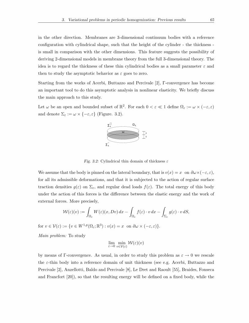
3. Variational problems in periodic homogenization: Previous results 65
in the other direction. Membranes are 3-dimensional continuum bodies with a reference
configuration with cylindrical shape, such that the height of the cylinder - the thickness -
is small in comparison with the other dimensions. This feature suggests the possibility of
deriving 2-dimensional models in membrane theory from the full 3-dimensional theory. The
idea is to regard the thickness of these thin cylindrical bodies as a small parameter ε and
then to study the asymptotic behavior as ε goes to zero.
Starting from the works of Acerbi, Buttazzo and Percivale [2], Γ-convergence has become
an important tool to do this asymptotic analysis in nonlinear elasticity. We briefly discuss
the main approach to this study.
Let ω be an open and bounded subset of R2. For each 0 < ε ≪ 1 define Ωε := ω × (−ε, ε)and denote Σε := ω × −ε, ε (Figure. 3.2).
εΣ
εΣ
εε
Ω ε
ω
−
+
Fig. 3.2: Cylindrical thin domain of thickness ε
We assume that the body is pinned on the lateral boundary, that is v(x) = x on ∂ω×(−ε, ε),for all its admissible deformations, and that it is subjected to the action of regular surface
traction densities g(ε) on Σε, and regular dead loads f(ε). The total energy of this body
under the action of this forces is the difference between the elastic energy and the work of
external forces. More precisely,
W(ε)(v) :=
∫
Ωε
W (ε)(x,Dv) dx−∫
Ωε
f(ε) · v dx−∫
Σε
g(ε) · v dS,
for v ∈ V(ε) := v ∈W 1,p(Ωε; R3) : v(x) = x on ∂ω × (−ε, ε).
Main problem: To study
limε→0
minv∈V(ε)
W(ε)(v)
by means of Γ-convergence. As usual, in order to study this problem as ε → 0 we rescale
the ε-thin body into a reference domain of unit thickness (see e.g. Acerbi, Buttazzo and
Percivale [2], Anzellotti, Baldo and Percivale [8], Le Dret and Raoult [55], Braides, Fonseca
and Francfort [20]), so that the resulting energy will be defined on a fixed body, while the

3. Variational problems in periodic homogenization: Previous results 66
dependence on ε turns out to be explicit in the transverse derivative. For this, we consider
the change of variables
Ωε → Ω := ω × I, (x1, x2, x3) 7→(
x1, x2,1
εx3
)
,
−
−
+
+
εε
Ωε
3
α
α =1,2
x
x
ω1
1
ΩΣ
Σ
Σ
Σε
ε
ω
Fig. 3.3: Rescaled domain of unit thickness
and define u(xα, x3/ε) = v(xα, x3) on the rescaled cylinder Ω, where I := (−1, 1) and
xα := (x1, x2) is the in-plane variable. We denote Σ := ω × −1, 1 (Figure. 3.3).
It is well known that membrane theory arises at the order ε of a formal asymptotic expansion
(see Fox, Raoult and Simo [52]), provided that the body forces are of order 1 and the surface
loadings are of order ε. Since this energy is of order ε, we divide the total energy by ε and
in addition we assume that
f(ε)(xα, εx3) = f(xα, x3),
g(ε)(xα, εx3) = ε g(xα, x3),
where f ∈ Lp′(Ω; R3), g ∈ Lp
′(Σ; R3) (1/p + 1/p′ = 1). If Wε(xα, x3; ·) = W (ε)(xα, εx3; ·),
for fixed ε minimizing W(ε) on V(ε) is equivalent to minimizing
Wε(u) :=W(ε)(v)
ε=
∫
ΩWε
(
x,∇αu(x)∣
∣
∣
1
ε∇3u(x)
)
dx−∫
Ωf · u dx−
∫
Σg · u dS
on Vε := u ∈ W 1,p(Ω; R3) : u(x) = (xα, εx3) on ∂ω × I. We recall that for ξ ∈ R3×2 and
z ∈ R3, (ξ|z) denote the matrix whose first two columns are those of ξ and the last one is
z; ∇α = (∇1,∇2).
Main step: To study
Γ(Lp(Ω))-limε→0
Wε.

3. Variational problems in periodic homogenization: Previous results 67
3.2.1 The case Wε(u) =
∫
Ω
W
(
x,xα
ε,∇αu
∣
∣
∣
1
ε∇3u
)
dx
The motivation to study this case comes from the works of Braides, Fonseca and Francfort
[20], of Babadjian and Francfort [11] and from Theorem 4.1.1.
Starting point: In [20] Braides, Fonseca and Francfort derived a homogenization result for
energiesWε(x; ξ) = W (x3, xα/ε, ξ). Namely, under the hypotheses thatW is a Caratheodory
function satisfying standard coerciveness and growth conditions, they proved that if
Wε(u) =
∫
ΩW
(
x3,xαε,∇αu
∣
∣
∣
1
ε∇3u
)
dx
then
Γ(Lp(Ω))- limε→0
Wε(u) = 2
∫
ωWhom(∇αu) dxα
for all u ∈W 1,p(ω; R3) ≡
u ∈W 1,p(Ω; R3) : D3u(x) = 0 for a.e.x ∈ Ω
, where
Whom(ξ) := limT→+∞
infφ
1
2T 2
∫
(0,T )2×IW(
y3, yα, ξ + ∇αφ(y)|∇3φ(y))
dy
φ ∈W 1,p((0, T )2 × I; R3), φ = 0 on ∂(0, T )2 × I
. (3.10)
Their analysis is based on a compactness property for a family of energies of the form
Wε(x, ξ). We state here this result since it is important for our applications in Chapter 5.2
Theorem 3.2.1. (Theorem 2.5 in [20]) Let ω be an open bounded subset of R2 and let
Ω := ω × I. Let Wε : Ω × R3×3 → [0,∞) be a family of Caratheodory functions such that
for a.e. x ∈ Ω and any ξ ∈ R3×3
β|ξ|p 6 Wε(x, ξ) 6 C(1 + |ξ|p), 0 < β 6 C, 1 < p <∞.
For each ε > 0 define Wε : Lp(Ω; R3) ×A(ω) → [0,∞) by
Wε(u;A) :=
∫
A×IWε
(
x,Dαu(x)∣
∣
∣
1
εD3u(x)
)
dx if u ∈W 1,p(A× I; R3),
∞ otherwise.
2 In [20] the authors prove a more general result for thin films with varying profiles. For our purposes it
is enough to present this simpler case.

3. Variational problems in periodic homogenization: Previous results 68
Let
Wε(u;A) := infuε
lim infε→0
Wε(uε;A) : uε → u in Lp(A× I; R3)
.
Then every sequence εn ↓ 0 admits a subsequence εnjj ≡ εjj such that Wεj( · ;A) is the
Γ(Lp(A × I))-limit of Wεj( · ;A)j for all A ∈ A(ω). Further there exists a Caratheodory
function Wεj : ω × R3×2 → R such that
Wεj(u;A) = 2
∫
AWεj(xα, Dαu(xα)) dxα, (3.11)
for all A ∈ A(ω) and all u ∈W 1,p(A; R3).
The proof of Theorem 3.2.1 is based on the Direct Method of Γ-convergence. In a first step
the authors derive a useful version of Proposition 2.5.13 that will allow us the matching of
recovering sequences in the lateral boundary of open sets A × I, with A ⊂ ω. Its proof is
based on De Giorgi’s slicing argument and the possibility of considering cut-off functions
independent on the transverse direction of the thin film.
Lemma 3.2.2. (Lemma 2.6 in [20]) Under the hypotheses of Theorem 3.2.1 on Wε, let A ∈A(ω), u ∈W 1,p(A; R3), and let εj ↓ 0 be a sequence for which Γ(Lp(A× I))- lim
j→∞Wεj
(u;A)
exists. Then there exists wjj ⊂ W 1,p(A × I; R3) and a sequence of compact sets of A,
Kjj, such that
Γ(Lp(A× I))- limj→∞
Wεj(u;A) = lim
j→∞Wεj
(wj , A)
and wj = u in (A \Kj) × I.
In Chapter 5 we study the asymptotic behavior of a heterogeneous ε-thin film whose mi-
crostructure oscillates on a scale that is comparable to that of the thickness of the domain
(see Figure 3.4). We propose in Theorem 5.1.1 to establish a dimensional reduction and ho-
mogenization result, where both scales are identical, by adding in the stored energy density
an explicit dependence on the in-plane variable xα. Namely, we assume that
Wε(x; ξ) = W(
x,xαε, ξ)
.
We seek to find the Γ(Lp(Ω))-limit of the following family of energies
Wε(u) :=
∫
ΩW
(
x,xαε,∇αu(x)
∣
∣
∣
1
ε∇3u(x)
)
dx

3. Variational problems in periodic homogenization: Previous results 69
ε
ε
Fig. 3.4: Thin domain with periodic structure in the in-plane direction
for u ∈ W 1,p(Ω; R3), and some function W : Ω × R2 × R3×3 → R whose hypotheses will
be introduced later(
in this case in the reference configuration Ωε we have W(ε)(x, ξ) =
W (xα,xε , ξ)
)
.
Two features differentiate our approach from what is available in most of the literature in
the subject (see Shu [75] and Braides, Fonseca and Francfort [20]). The first one is the
use of two-scale techniques as in Theorem 4.1.1. The second one is based on a decoupling
argument used by Babadjian and Francfort [11] to derive a nonlinear membrane model for
stored energy densities of the form W (x, ξ) generalizing the case where Wε(x, ξ) ≡W (x3, ξ)
that was studied in Braides, Fonseca and Francfort [20]. This decoupling procedure is
necessary to take into account the different nature of the two variables yα and xα that
appear in the structure of the limit functional (see (5.24) below).
3.2.2 The case Wε(u) =
∫
Ω
W
(
x,x
ε,xα
ε2,∇αu
∣
∣
∣
1
ε∇3u
)
dx
In Theorem 5.2.1 we want to study the asymptotic analysis of ε-thin elastic bodies whose
microstructure is periodic of period ε in the in-plane direction and periodic of period ε2 in
all directions. To take into account these heterogeneities, our goal is to study the sequence
of energies
Wε(x; ξ) = W(
x,x
ε,xαε2, ξ)
(
in this case in the reference configuration Ωε we have W(ε)(x, ξ) = W (xα,x3ε ,
xα
ε ,xε2, ξ))
.
We seek to find the Γ(Lp(Ω))-limit of the following family of energies
Wε(u) :=
∫
ΩW
(
x,x
ε,xαε2,∇αu(x)
∣
∣
∣
1
ε∇3u(x)
)
dx,
for u ∈W 1,p(Ω; R3), and for some function W : Ω×R3 ×R2 ×R3×3 → R whose hypotheses
will be introduced later. As a corollary, we derive a homogenization result for heterogeneous

3. Variational problems in periodic homogenization: Previous results 70
ε-thin films of periodic structure of period ε in the in-plane variable xα and of period ε2 in
the transverse direction x3. That is, we derive an homogenization formula for a family of
energies
Wε(u) :=
∫
ΩW
(
x,x
ε,∇αu(x)
∣
∣
∣
1
ε∇3u(x)
)
dx
for u ∈W 1,p(Ω; R3). Integral functionals of the form
∫
ΩW
(
xαε2,∇αv
∣
∣
∣
1
ε∇3v
)
dx,
have been studied in Shu [75] (Theorem 5) under different length scales for the film thickness
and the material microstructure. As far as we know there have no been previous results
that allow for homogenization in the transverse direction of the film.

Part II
MAIN RESULTS

4. Γ-CONVERGENCE OF FUNCTIONALS WITH
PERIODIC INTEGRANDS
The main goal of this chapter is to characterize the asymptotic behavior of a family of
multiple scale integral functionals whose integrands have periodicity properties.
From now on, unless otherwise specified, C will denote a generic constant, and for every
a ∈ RN and δ > 0 we write Q(a, δ) := a + δQ ≡ (a, δ)N , where Q := (0, 1)N . Throughout
this chapter Ω stands for an open bounded set in RN with N > 1.
4.1 An approach by 2-scale convergence
This section is devoted to proving the following result.
Theorem 4.1.1. Let f : Ω × RN × Rd×N → R be a function such that
(H1) f(x, ·, ·) is continuous a.e. x ∈ Ω;
(H2) f(·, y, ξ) is LN -measurable for all y ∈ RN and all ξ ∈ Rd×N ;
(H3) f(x, ·, ξ) is Q-periodic for a.e. x ∈ Ω and for all ξ ∈ Rd×N ;
(H4) there exist a real number p > 1 and a constant β > 0 such that
|ξ|pβ
− β 6 f(x, y, ξ) 6 β(1 + |ξ|p),
for a.e. x ∈ Ω, for all y ∈ RN and all ξ ∈ Rd×N .
For each ε > 0 define the functional Iε : Lp(Ω; Rd) → [0,∞] by

4. Γ-convergence of functionals with periodic integrands 74
Iε(u) :=
∫
Ωf(
x,x
ε,∇u(x)
)
dx if u ∈W 1,p(Ω; Rd),
∞ otherwise.
(4.1)
If u ∈ Lp(Ω; Rd) then
Ihom(u) := Γ(Lp(Ω))- limε→0
Iε(u) =
∫
Ωfhom(x,∇u(x)) dx if u ∈W 1,p(Ω; Rd),
∞ otherwise,
(4.2)
where the integrand fhom is given by
fhom(x, ξ) := limT→∞
infφ
1
TN
∫
(0,T )N
f(x, y, ξ + ∇φ(y)) dy, φ ∈W 1,p0 ((0, T )N ; Rd)
(4.3)
for a.e. x ∈ Ω and for all ξ ∈ Rd×N . It turns out that fhom is (equivalent to) a Caratheodory
function and satisfies p-coercivity and p-growth conditions similar to those of f . Moreover
fhom(x, · ) is quasiconvex for a.e. x ∈ Ω.
Theorem 4.1.1 was obtained in collaboration with I. Fonseca [12], and the main idea of its
proof is to use the Direct Method of the Calculus of Variations (see Section 2.5.2) combined
with the integral representation theorem of Buttazzo and Dal Maso (Theorem 2.4.1) to
derive the existence of Γ-converging (sub)sequences to an abstract integral functional. Then
the idea is to use arguments of two-scale convergence to derive an upper bound for the
integrand of this functional. To get the other bound we use the fact that, under hypotheses
(H1)-(H4), the integrand f is “uniformly continuous up to a small error”. Indeed, since
f is a Caratheodory integrand, Scorza-Dragoni’s Theorem (Theorem 2.3.26) implies that
the restriction of f to K × RN × Rd×N is continuous, for some compact set K ⊂ Ω whose
complement has arbitrarily small Lebesgue measure. Then the periodicity of f with respect
to its second variable leads f to be uniformly continuous on K × RN × B, for some closed
ball B of Rd×N of sufficiently large radius. Finally, to ensure that the energy remains
arbitrarily small on the complement of K and on the set of x’s such that the gradient of
the deformation does not belong to B, we use the Decomposition Lemma (Theorem 2.2.16)
which allows us to select minimizing sequences with pth-equi-integrable gradients. Thus, in
view of the p-growth character of the integrand, the energy over sets of arbitrarily small
Lebesgue measure tends to zero.

4. Γ-convergence of functionals with periodic integrands 75
Like for quasiconvex envelopes, there are very few explicit examples of homogenized densities
in the literature. A classical explicit derivation of the function fhom for elliptic operators in
the homogeneous case, that is, for integrands f that do not depend on the variable x, can
be found in De Giorgi and Spagnolo [41]. We present a classical example that can be found
in the book of Dal Maso [35] (see references therein for more examples).
Example. Let N = 1 and let f(y, ξ) := a(y)|ξ|p for (y, ξ) ∈ R2 and 1 < p <∞, where a is a
measurable and Q-periodic function, such that for all y ∈ R
β 6 a(y) 6 C, 0 < β 6 C.
Then fhom(ξ) = ahom|ξ|p where
ahom :=
(
∫ 1
0
(
1
a
)p/p−1)1−p
.
Remark 4.1.2. By hypothesis (H1) and (H2) the integrand f is of Caratheodory-type and
this ensures that f(x, ·, ·) is a Borel function for a.e. x ∈ Ω (see Proposition 2.3.27; in
particular the integral in (4.1) is well defined). Moreover, by hypothesis (H4) replacing f by
f+β we may assume that f is nonnegative almost everywhere. As a consequence of these two
remarks, in the sequel, without loss of generality, we may assume that f is a positive Borel
function such that hypotheses (H1), (H3) and (H4) hold for every (x, y, ξ) ∈ Ω×RN×Rd×N .
Two more remarks are worthy of note (see Muller [66] and Braides and Defranceschi [19];
see also Lemma 4.1.5 and Lemma 4.1.10 below). First, it can be seen that for a.e. x ∈ Ω
and for all ξ ∈ Rd×N
fhom(x, ξ) = infT∈N
infφ
1
TN
∫
(0,T )N
f(x, y, ξ + ∇φ(y)) dy, φ ∈W 1,p0 ((0, T )N ; Rd)
(4.4)
and
fhom(x, ξ) = infT∈N
infφ
1
TN
∫
(0,T )N
f(x, y, ξ + ∇φ(y)) dy, φ ∈W 1,pper((0, T )N ; Rd)
, (4.5)
Secondly, we observe that under the additional hypothesis that f(x, y, ·) is convex for a.e.
x and for all y (in which case (H1) is equivalent to requiring that f(x, ·, ξ) is continuous for
a.e. x and for all ξ), equalities (4.4) and (4.5) simplify to read, respectively,
fhom(x, ξ) = infφ
∫
Qf(x, y, ξ + ∇φ(y)) dy, φ ∈W 1,p
0 ((0, 1)N ; Rd)
(4.6)

4. Γ-convergence of functionals with periodic integrands 76
and
fhom(x, ξ) = infφ
∫
Qf(x, y, ξ + ∇φ(y)) dy, φ ∈W 1,p
per((0, 1)N ; Rd)
. (4.7)
Moreover, by hypothesis (H1) and by Lemma 2.3.28, equalities (4.3)-(4.7) hold if the ad-
missible test functions are taken in any smooth dense subset of W 1,p0 ((0, T )N ; Rd) and
W 1,pper((0, T )N ; Rd), respectively.
As a consequence of Theorem 4.1.1, Proposition 2.5.13 and Theorem 2.5.11 we get the
convergence of (almost) minimizers of Iεε.
Corollary 4.1.3. Under hypotheses (H1)-(H4) the functional Ihom defined in (4.2) has a
minimum on Vϕ := u ∈W 1,p(Ω) : u− ϕ ∈W 1,p0 (Ω), ϕ ∈W 1,p(Ω) and
minu∈Vϕ
Ihom(u) = limε→0
infu∈Vϕ
Iε(u).
Moreover, given two sequences εn ↓ 0 and unn ⊂ Vϕ) such that
limn→∞
Iεn(un) = limn→∞
infu∈Vϕ
Iεn(u),
then (up to subsequence) unn is W 1,p-weakly convergent to a minimum for the functional
Ihom on Vϕ.
4.1.1 Properties of the homogenized density
In this section we turn our attention to the main properties of the function fhom for later use
in the proof of Theorem 4.1.1. Most of these properties can be deduced from previous works
(see references below), however we present alternative proofs for the sake of completeness.
By Remark 4.1.2 we restrict our analysis to the case where f is a positive Borel function
such that hypotheses (H1), (H3) and (H4) hold for every (x, y, ξ) ∈ Ω × RN × Rd×N .
We start by showing that the limit in (4.3) is well defined. The argument is analogous
to that used in Bouchitte, Fonseca and Mascarenhas [23] and relies on Lemma A.1 in the
Appendix.
Lemma 4.1.4. For all (x, ξ) ∈ Ω × Rd×N there exists
limT→∞
infφ
1
TN
∫
(0,T )N
f(x, y, ξ + ∇φ(y)) dy, φ ∈W 1,p0 ((0, T )N ; Rd)
. (4.8)
4. Γ-convergence of functionals with periodic integrands 77
Proof. (see also Braides and Defranceschi [19]) Let (x, ξ) ∈ Ω × Rd×N and let
S(A) := infφ
∫
Af(x, y, ξ + ∇φ(y)) dy : φ ∈W 1,p
0 (A; Rd)
for A ∈ A(RN ). Under the above assumptions on f the function S : A(RN ) → [0,∞) is
well defined, and it satisfies the hypotheses of Lemma A.1 with T = ZN and M = 1. Hence
we conclude that the limit
limT→∞
S((0, T )N )
TN,
or equivalently (4.8), exists.
We now want to show that fhom is a Caratheodory integrand (see Definition 2.3.25) so that
the functional Ihom in (4.2) is well defined. We start by noting the following result.
Lemma 4.1.5. Let fhom, fhom : Ω × Rd×N → [0,∞) be defined, respectively, by
fhom(x, ξ) := infT∈N
infφ
1
TN
∫
(0,T )N
f(x, y, ξ + ∇φ(y)) dy, φ ∈W 1,p0 ((0, T )N ; Rd)
and
fhom(x, ξ) := infT∈N
infφ
1
TN
∫
(0,T )N
f(x, y, ξ + ∇φ(y)) dy, φ ∈W 1,pper((0, T )N ; Rd)
,
for all (x, ξ) ∈ Ω × Rd×N. Then the relations fhom = fhom = fhom hold.
Proof. Let (x, ξ) ∈ Ω × Rd×N . We first show that fhom(x, ξ) = fhom(x, ξ). It is clear
that fhom(x, ξ) > fhom(x, ξ). To prove the other inequality, fixed δ > 0 let S ∈ N and
ϕ ∈W 1,p0 ((0, S)N ; Rd) be such that
fhom(x, ξ) + δ >1
SN
∫
(0,S)N
f(x, y, ξ + ∇ϕ(y)) dy. (4.9)
Extend ϕ periodically to RN with period S. Using Riemann-Lebesgue’s Lemma (Lemma
2.6.2)
1
SN
∫
(0,S)N
f(x, y, ξ + ∇ϕ(y)) dy = limε→0
1
SN
∫
(0,S)N
f(
x,y
ε, ξ + ∇ϕ
(y
ε
))
dy
= limε→0
εN
SN
∫
(
0,Sε
)Nf(x, z, ξ + ∇θε(z)) dz, (4.10)

4. Γ-convergence of functionals with periodic integrands 78
where θε(z) := 1εϕ(εz) ∈W 1,p
0
(
(
0, Sε)N
; Rd)
. Therefore from (4.9) and (4.10)
fhom(x, ξ) + δ > limε→0
infθ
εN
SN
∫
(0,Sε)N
f(x, z, ξ + ∇θ(z)) dz, θ ∈W 1,p0
((
0,S
ε
)N; Rd
)
= fhom(x, ξ).
Letting δ → 0 we conclude that
fhom(x, ξ) > fhom(x, ξ).
Finally we show that fhom(x, ξ) = fhom(x, ξ) (see also Braides [19] and Muller [66] for an
alternative justification). It is clear that fhom(x, ξ) > fhom(x, ξ). To verify the opposite
inequality, fix δ > 0 and take S ∈ N and a smooth function ϕ ∈ W 1,pper
(
(0, S)N ; Rd)
such
that
fhom(x, ξ) + δ >1
SN
∫
(0,S)N
f(x, y, ξ + ∇ϕ(y)) dy. (4.11)
By hypothesis (H3) the function f(x, ·, ξ + ∇ϕ(·)) is (0, S)N -periodic, and thus
1
SN
∫
(0,S)N
f(x, y, ξ + ∇ϕ(y)) dy = limε→0
∫
Qf(
x,y
ε, ξ + ∇ϕ
(y
ε
))
dy
= limε→0
∫
Qf(
x,y
ε, ξ + ∇ψε(y)
)
dy, (4.12)
where ψε(y) := εϕ(
yε
)
. For each ε > 0 define
Qε :=
y ∈ Q : dist(y, ∂Q) > ε
.
Take θε ∈ C∞c (Q) with θε ∈ [0, 1] such that θε = 1 on Qε and ||∇θε||L∞ 6 Cε−1. Then
limε→0
∫
Qf(
x,y
ε, ξ + ∇(θεψε)(y)
)
dy = limε→0
∫
Qε
f(
x,y
ε, ξ + ∇ψε(y)
)
dy, (4.13)
since by the p-growth condition in (H4) we have∫
Q\Qε
f(
x,y
ε, ξ + ∇(θεψε)(y)
)
dy
6 C
∫
Q\Qε
(
1 + |ξ|p + |∇ψε(y)|p + ε−p|ψε(y)|p)
dy
= C[
|Q \Qε| +∫
Q\Qε
∣
∣
∣∇ϕ(y
ε
)∣
∣
∣
pdy +
∫
Q\Qε
∣
∣
∣ϕ(y
ε
)∣
∣
∣
pdy]
→ 0.

4. Γ-convergence of functionals with periodic integrands 79
Hence by (4.11)-(4.13), defining φε(y) := 1ε (θεψε)(εy) ∈W 1,p
0
((
0, 1ε
)N; RN
)
, we obtain
fhom(x, ξ) + δ > limε→0
∫
Qf(
x,y
ε, ξ + ∇(θεψε)(y)
)
dy
> limε→0
εN∫
(
0, 1ε
)Nf(
x, y, ξ + ∇φε(y))
dy
> fhom(x, ξ).
Letting δ → 0 we get fhom(x, ξ) > fhom(x, ξ).
The measurability of fhom follows as a consequence.
Lemma 4.1.6. The function fhom(·, ξ) is measurable for all ξ ∈ Rd×N .
Proof. Let ξ ∈ Rd×N . By Lemma 4.1.5 we can write
fhom(x, ξ) = infT∈N
infφ∈ST
fT, φ(x)
where
fT, φ(x) :=
∫
Tf(x, y, ξ + ∇φ(z)) dz
for x ∈ Ω, and ST is a countable subset of C∞c ((0, T )N ; Rd) dense in W 1,p
0 ((0, T )N ; Rd). By
Tonelli’s Theorem the functions fT, φ are measurable, and so is fhom(·, ξ) as the infimum of
a countable family of measurable functions.
Our next objective is to show that fhom(x, ·) is continuous for all x ∈ Ω. We are not able
to prove this directly unless f satisfy a p-Lipschitz condition as in (2.9). As quasiconvex
functions satisfy inequality (2.9) (see Proposition 2.3.15), the first step will be to show that
fhom = (Qf)hom where Qf : Ω × RN × Rd×N → R denotes the usual quasiconvexification
of f with respect to the last variable ξ, that we know to be quasiconvex in ξ (see Theorem
2.3.19). We remark that
Qf(x, y, ξ) = infφ
∫
Qf(x, y, ξ + ∇φ(z)) dz : φ ∈W 1,p
0 (Q; Rd)
(4.14)
for all (x, y, ξ) ∈ Ω × RN × Rd×N (see Lemma 2.3.23) and that consequently Qf satisfies
conditions (H3) and (H4). The following properties of Qf are of interest for the argument
that follows.
4. Γ-convergence of functionals with periodic integrands 80
Lemma 4.1.7. We have that
i) Qf(x, ·, ·) is continuous for all x ∈ Ω;
ii) Qf(·, y, ξ) is measurable for all (y, ξ) ∈ RN × Rd×N ;
iii) (Qf)hom(x, ξ) := lim infT→∞
inf
1TN
∫
(0,T )N
Qf(x, y, ξ + ∇φ(y)) dy, φ ∈W 1,p0 ((0, T )N ; Rd)
= limT→∞
inf
1TN
∫
(0,T )N
Qf(x, y, ξ + ∇φ(y)) dy, φ ∈W 1,p0 ((0, T )N ; Rd)
for all (x, ξ) ∈ Ω × RN × Rd×N .
iv) (Qf)hom(x, ξ) = fhom(x, ξ) for all (x, ξ) ∈ Ω × Rd×N .
Proof. i) The upper semicontinuity of Qf(x, ·, ·) for x ∈ RN follows from equality (4.14) and
hypothesis (H1), while its lower semicontinuity can be obtained by an argument analogous
to that of Lemma 2.3.24.
ii) The proof is identical to that of Lemma 4.1.6 above.
iii) Is a consequence of identities i) and ii), the coerciveness, growth and periodicity prop-
erties of Qf , and of Lemma 4.1.4.
iv) Let (x, ξ) ∈ Ω×Rd×N . Obviously fhom(x, ξ) > (Qf)hom(x, ξ). Let us prove the converse
inequality. Let n ∈ N and let Tn ∈ N and φn ∈W 1,p0 ((0, Tn)
N ; Rd) be such that
(Qf)hom(x, ξ) +1
n>
1
TNn
∫
(0,Tn)N
Qf(x, y; ξ + ∇φn(y)) dy.
Thus
(Qf)hom(x, ξ) > lim supn→∞
1
TNn
∫
(0,Tn)N
Qf(x, y; ξ + ∇φn(y)) dy. (4.15)
To compare (4.15) with fhom(x, ξ) we apply the Acerbi and Fusco Relaxation Theorem
(Theorem 2.3.30) and the Decomposition Lemma (Lemma 2.2.16). As a consequence of
Theorem 2.3.30, for every n fixed there exists a sequence φn,kk ⊂W 1,p((0, Tn)N ; Rd) such
that φn,k kφn in W 1,p((0, Tn)
N ; Rd) and
1
TNn
∫
(0,Tn)N
Qf(x, y; ξ + ∇φn(y)) dy = limk→∞
1
TNn
∫
(0,Tn)N
f(x, y; ξ + ∇φn,k(y)) dy. (4.16)

4. Γ-convergence of functionals with periodic integrands 81
By Lemma 2.2.16 we can now find a subsequence (still denoted by φn,kk) and a sequence
ψn,kk ⊂W 1,∞0 (RN ; Rd) such that ψn,k φn in W 1,p((0, Tn)
N ; Rd) with
|∇ψn,k|p equi-integrable (4.17)
and
LNy ∈ (0, Tn)N : ψn,k(y) 6= φn,k(y) −→
k→∞0. (4.18)
As f is nonnegative, by (4.17) and (4.18)
limk→∞
1
TNn
∫
(0,Tn)N
f(x, y; ξ + ∇φn,k(y)) dy
> lim supk→∞
1
TNn
∫
y∈(0,Tn)N : ψn,k(y)=φn,k(y)f(x, y; ξ + ∇ψn,k(y)) dy
= lim supk→∞
1
TNn
∫
(0,Tn)N
f(x, y; ξ + ∇ψn,k(y)) dy. (4.19)
Thus from (4.15), (4.16) and (4.19)
(Qf)hom(x, ξ) > lim supn→∞
lim supk→∞
1
TNn
∫
(0,Tn)N
f(x, y, ξ + ∇ψn,k(y)) dy > fhom(x, ξ).
We are now in a position to prove the continuity property of fhom.
Lemma 4.1.8. The function fhom(x, ·) (or equivalently (Qf)hom(x, ·)) is continuous for all
x ∈ Ω.
Proof. (see also Braides [19]) Fix x ∈ Ω. Let ξ ∈ Rd×N and ξn → ξ in Rd×N . We wish to
show that
fhom(x, ξ) = limn→∞
fhom(x, ξn).
We first establish that (upper semicontinuity)
fhom(x, ξ) > lim supn→∞
fhom(x, ξn). (4.20)
Fixed δ > 0, choose S ∈ N and by density a function ϕ ∈ C∞0 ((0, S)N ; Rd) such that
fhom(x, ξ) + δ >1
SN
∫
(0,S)N
f(x, y, ξ + ∇ϕ(y)) dy
=1
SNlimn→∞
∫
(0,S)N
f(x, y, ξn + ∇ϕ(y)) dy
> lim supn→∞
fhom(x, ξn),

4. Γ-convergence of functionals with periodic integrands 82
as a consequence of Lemmas 2.1.15 and 4.1.5. Letting δ → 0 we get (4.20).
We show now the converse inequality (lower semicontinuity), i.e.
fhom(x, ξ) 6 lim infn→∞
fhom(x, ξn). (4.21)
We start by remarking that fhom(x, ξn) = (Qf)hom(x, ξn) for all n ∈ N (property iv) in
Lemma 4.1.7). Given n ∈ N, consider Tn ∈ N (Tn ր ∞) and φn ∈ W 1,p0 ((0, Tn)
N ; Rd) such
that
fhom(x, ξn) +1
n>
1
TnN
∫
(0,Tn)N
Qf(x, y, ξn + ∇φn(y)) dy
=
∫
(0,1)N
Qf(x, Tny, ξn + ∇φn(Tny)) dy
=
∫
(0,1)N
Qf(x, Tny, ξn + ∇ψn(y)) dy, (4.22)
where ψn(y) := 1Tnφn(Tny), ψn ∈ W 1,p
0 ((0, 1)N ; Rd). We note that by the p-coervivity con-
dition of (Qf) the sequence ||∇ψn||Lp((0,1)N ;Rd) is bounded. We write∫
(0,1)N
Qf(x, Tny, ξn + ∇ψn(y)) dy
=
∫
(0,1)N
Qf(x, Tny, ξn + ∇ψn(y)) −Qf(x, Tny, ξ + ∇ψn(y)) dy (4.23)
+
∫
(0,1)N
Qf(x, Tny, ξ + ∇ψn(y)) dy.
Our task now is to show that the term (4.23) goes to zero as n goes to infinity. As ξn → ξ
and the sequence ||∇ψn||Lp((0,1)N ;Rd) is bounded, using the p-Lipschitz condition (2.9) and
Holder Inequality we have
lim supn→∞
∫
(0,1)N
|Qf(x, Tny, ξn + ∇ψn(y)) −Qf(x, Tny, ξ + ∇ψn(y)) | dy
6 C lim supn→∞
∫
(0,1)N
(
1 + |ξn + ∇ψn(y)|p−1 + |ξ + ∇ψn(y)|p−1)
|ξn − ξ| dy
6 C lim supn→∞
∫
(0,1)N
(
1 + |∇ψn(y)|p−1)
|ξn − ξ| dy
6 C limn→∞
|ξn − ξ| = 0,
which, together with (4.22), leads to
fhom(x, ξn) +1
n> lim sup
n→∞
∫
(0,1)N
Qf(x, Tny, ξ + ∇ψn(y)) dy > (Qf)hom(x, ξ) = fhom(x, ξ).

4. Γ-convergence of functionals with periodic integrands 83
Inequality (4.21) holds letting n→ ∞.
By Lemmas 4.1.6 and 4.1.8, we conclude that fhom is a Caratheodory integrand and thus
Ihom is well defined.
Remark 4.1.9. We note that fhom satisfies analogous growth and coercivity conditions to
the ones of f , which, together with the continuity properties of fhom, imply by standard
arguments (approximation ofW 1,p by piecewise affine functions together with the invariance
of the domain of fhom) that this function is quasiconvex with respect to the last variable.
We will show next that in the convex case it is enough to consider one cell period for the
definition of fhom (4.3) (see also Braides [19] or Muller [66]). We define for all (x, ξ) ∈Ω × Rd×N
f⋆hom(x, ξ) = infφ
∫
Qf(x, y, ξ + ∇φ(y)) dy, φ ∈W 1,p
0 ((0, 1)N ; Rd)
and
f⋆⋆hom(x, ξ) = infφ
∫
Qf(x, y, ξ + ∇φ(y)) dy, φ ∈W 1,p
per((0, 1)N ; Rd)
.
Lemma 4.1.10. Assume, in addition to the hypotheses on f , that f(x, y, ·) is convex for
all (x, y) ∈ Ω × RN . Then
f⋆hom = f⋆⋆hom = fhom.
Proof. (see Braides [19] and Muller [66] for an alternative proof). Equality f⋆hom = f⋆⋆hom is
proven by an argument analog to that of the proof of Lemma 4.1.5.
We show that f⋆hom = fhom. Let (x, ξ) ∈ Ω × Rd×N . By definition f⋆hom(x, ξ) > fhom(x, ξ).
To prove the opposite inequality, for each n ∈ N take Tn ∈ N and a function φn ∈W 1,p
0 ((0, Tn)N ; Rd) such that
fhom(x, ξ) + 1n > 1
TNn
∫
(0,Tn)N
f(x, y, ξ + ∇φn(y)) dy
=
∫
Qf(x, Tny, ξ + ∇ψn(y)) dy,
(4.24)
where ψn(y) := 1Tnφn(Tny), ψn ∈ W 1,p
0 (Q; Rd). By the p-growth condition in (H4) the
sequence ||∇ψn||Lp(Q;Rd)n is bounded, and so is ||ψn||W 1,p(Q;Rd)n by Poincare Inequality.

4. Γ-convergence of functionals with periodic integrands 84
Hence, there exists a subsequence (still denoted by ψnn) such that
ψnW 1,p
ψ
for some ψ = ψ(y) ∈ W 1,p0 (Q; Rd). As a consequence, by Theorem 2.6.7 and up to a
subsequence
ψn2s ψ
and
∇ψn 2s ∇ψ + ∇zψ
for some ψ = ψ(y, z) ∈ Lp(
Q;W 1,pper(Q; Rd)
)
. We divide the rest of the proof in two steps.
Step 1. We follow an argument of Allaire [4] assuming in addition that
(H5)∂f∂η (x, y, η) exists for all (x, y, η) ∈ Ω × RN × Rd×N .
By inequalities (2.5) and (2.6), and by the p-growth condition in (H4) there exists a constant
C > 0 such that for all (x, y, η) ∈ Ω × RN × Rd×N
∣
∣
∣
∂f
∂η(x, y, η)
∣
∣
∣6 C
[
1 + |η|p−1]
. (4.25)
Let ϕ = ϕ(y, z) ∈ C∞c
(
Q;C∞per(Q; Rd×N )
)
. Since f is convex in the last variable then by
inequality (2.5)∫
Qf(
x, Tny, ξ + ∇ψn(y))
dy >
∫
Qf(
x, Tny, ξ + ϕ(y, Tny))
dy
+
∫
Q
∂f
∂η
(
x, Tny, ϕ(y, Tny))
· (∇ψn(y) − ϕ(y, Tny)) dy,
(4.26)
for each n ∈ N. By Lemma 2.6.3, and as ∇ψn 2s ∇ψ +∇zψ (see Definition 2.6.5), we have
limn→∞
∫
Qf(
x, Tny, ξ + ϕ(y, Tny))
dy =
∫
Q
[
∫
Qf(
x, z, ξ + ϕ(y, z))
dz]
dy (4.27)
and
limn→∞
∫
Q
∂f
∂η
(
x, Tny, ϕ(y, Tny))
· (∇ψn(y) − ϕ(y, Tny)) dy
=
∫
Q
[
∫
Q
∂f
∂η
(
x, z, ϕ(y, z))
· (∇ψ(y) + ∇zψ(y, z) − ϕ(y, z)) dz]
dy.
(4.28)

4. Γ-convergence of functionals with periodic integrands 85
Therefore, from (4.26)-(4.28) we get
lim infn→∞
∫
Qf(
x, Tny, ξ + ∇ψn(y))
dy >
∫
Q
[ ∫
Qf(
x, z, ξ + ϕ(y, z))
dz
]
dy
+
∫
Q
[ ∫
Q
∂f
∂η
(
x, z, ϕ(y, z))
· (∇ψ(y) + ∇zψ(y, z) − ϕ(y, z)) dz
]
dy,
(4.29)
for all ϕ = ϕ(y, z) ∈ C∞c
(
Q;C∞per(Q; Rd×N )
)
. Let now ϕkk ⊂ C∞c
(
Q;C∞c (Q; Rd×N )
)
be a
convergent sequence to ∇ψ + ∇zψ in Lp(
Q×Q; Rd×N)
. In particular from (4.29) we get
lim infn→∞
∫
Qf(
x, Tny, ξ + ∇ψn(y))
dy >
∫
Q
[ ∫
Qf(
x, z, ξ + ϕk(y, z))
dz
]
dy
+
∫
Q
[ ∫
Q
∂f
∂η
(
x, z, ϕk(y, z))
· (∇ψ(y) + ∇zψ(y, z) − ϕk(y, z)) dz
]
dy,
(4.30)
for every k ∈ N. Inequality (4.25) and the growth conditions on f and ∂f∂η imply that we
can pass to the limit in (4.30) and get
lim infn→∞
∫
Qf(
x, Tny, ξ + ∇ψn(y))
dy >
∫
Q
[ ∫
Qf(
x, z, ξ + ∇ψ(y) + ∇zψ(y, z))
dz
]
dy.
(4.31)
By Jensen’s Inequality and Fubini’s Theorem, for each z ∈ Q∫
Qf(
x, z, ξ + ∇ψ(y) + ∇zψ(y, z))
dy > f(
x, z,
∫
Q
[
ξ + ∇ψ(y) + ∇zψ(y, z)]
dy)
= f(
x, z, ξ + ∇z
(
∫
Qψ(y, z) dy
))
. (4.32)
Thus, by (4.24), (4.31), (4.32), and once more Fubini’s Theorem
fhom(ξ) >
∫
Qf(
z, ξ + ∇z
(
∫
Qψ(y, z) dy
))
dz > f⋆⋆hom(ξ) = f⋆hom(ξ).
Step 2. We address now the general case. For each ε > 0 set ζε(η) := 1εN ζ
(
ηε
)
where
ζ ∈ C∞(Rd×N ) denotes the standard mollifier, that is,
ζ(η) :=
C exp(
1|η|2−1
)
if |η| < 1,
0 if |η| > 1,
4. Γ-convergence of functionals with periodic integrands 86
and the constant C is selected so that
∫
Rd×N
ζ(η) dη = 1. Let
fε(x, y, ξ) :=
∫
B(0,ε)ζε(η)f(x, y, ξ − η) dη
for all ε > 0 and all (x, y, ξ) ∈ Ω × RN × Rd×N . It is straightforward to show that fε
satisfies conditions (H1)-(H5). Fix δ > 0 and, by a density argument, let S ∈ N and
ψ ∈W 1,∞((0, S)N ; Rd) be such that
fhom(x, ξ) + δ >1
SN
∫
(0,S)N
f(x, y, ξ + ∇ψ(y)) dy.
Then
fhom(x, ξ) + δ > limε→0
1
SN
∫
(0,S)N
fε(x, y, ξ + ∇ψ(y)) dy,
and thus
fhom(x, ξ) + δ > lim supε→0
(fε)hom(x, ξ)
= lim supε→0
(fε)⋆⋆hom(x, ξ)
> f⋆⋆hom(x, ξ)
since fε is convex and fε > f for all ε > 0. Indeed, it is easy to show that fε is convex and
the last assertion is a consequence of the convexity of f and Jensen’s Inequality.
4.1.2 Proof of the main result
As in the previous subsection, by Remark 4.1.2 we may suppose that f is a positive Borel
function satisfying hypotheses (H1), (H3) and (H4) for every (x, y, ξ) ∈ Ω × RN × Rd×N .
Due to the p-coercivity condition in (H4), to prove Theorem 4.1.1 it suffices to show that
Γ(Lp(Ω))- limε→0
Iε(u) =
∫
Ωfhom(x, u(x),∇u(x)) dx, (4.33)
for all u ∈W 1,p(Ω; Rd), since
Γ(Lp(Ω))- limε→0
Iε(u) = ∞

4. Γ-convergence of functionals with periodic integrands 87
for all u ∈ Lp(Ω; RN ) \W 1,p(Ω; Rd). To prove identity (4.33) we use the Direct Method of
Γ- convergence. Accordingly, we start by localizing the functionals Iε in order to highlight
their dependence on the domain of integration, that is, we consider a family of functionals
Iε : Lp(Ω; Rd) ×A(Ω) → [0,∞] defined by
Iε(u;A) :=
∫
Af(
x,x
ε,∇u(x)
)
dx if u ∈W 1,p(A; Rd),
∞ otherwise.
Our goal is to show that
Γ(Lp(Ω))- limε→0
Iε(u,A) =
∫
Afhom(x,∇u(x)) dx, (4.34)
for all u ∈W 1,p(Ω; Rd) and A ∈ A(Ω). In particular (4.33) will follow by taking A = Ω.
The next step toward the proof of (4.34) is to establish a compactness property that ensures
the existence of Γ-converging subsequences of Iεε.
Proposition 4.1.11. For every sequence εnn of positive real numbers converging to zero
there exists a further subsequence εnjj ≡ εjj such that
Γ(Lp(A))- limj→∞
Iεj(·;A)(u) =: Iεj(u;A) (4.35)
exists for all u ∈W 1,p(Ω,Rd) and all A ∈ A(Ω).
The proof of this proposition follows an argument analog to the one used in Braides, Fonseca
and Francfort [20], but for completeness we present it here.
Let R be a countable collection of subsets of Ω such that, for any δ > 0 and any A ∈ A(Ω),
there exists a finite union CA of disjoint elements of R satisfying
CA ⊂ A,
LN (A) 6 LN (CA) + δ.
We may take R as the set of open squares with faces parallel to the axes, centered at points
x ∈ Ω∩QN and with rational edge lengths. We denote by R the countable collection of all
finite unions of elements of R, i.e.
R =
k⋃
i=1
Ci : k ∈ N, Ci ∈ R
.
4. Γ-convergence of functionals with periodic integrands 88
The next lemma is the starting point for the proof of Proposition 4.1.11.
Lemma 4.1.12. For every sequence εnn of positive real numbers converging to zero there
exists a further subsequence εnjj (depending on R) such that the Γ-limit
Γ(Lp(C))- limj→∞
Iεnj(·;C)(u) =: Iεnj
(u;C) (4.36)
exists for all u ∈W 1,p(Ω,Rd) and all C ∈ R.
Proof. Let C ∈ R. From Proposition 2.5.8 and as Lp(Ω; Rd) is separable there exist a
subsequence εnjj (depending on C) such that the Γ(Lp(C))-limit of Iεnj
(·;C) exists for
all u ∈ W 1,p(Ω,Rd). But then by a diagonalization procedure we can find a subsequence
εnjj (depending on R) such that (4.36) holds.
Let now εnn be a fixed sequence of positive real numbers converging to zero and εjj a
subsequence for which (4.36) holds.
Proof of Proposition 4.1.11. We wish to show that for all A ∈ A(Ω) and u ∈W 1,p(Ω,Rd)
inf
lim infj→∞
∫
Af(
x,x
εj,∇uj(x)
)
dx : uj ∈W 1,p(A,Rd), ujLp(A;Rd)−→ u
(4.37)
= inf
lim supj→∞
∫
Af(
x,x
εj,∇uj(x)
)
dx : uj ∈W 1,p(A,Rd), ujLp(A;Rd)−→ u
.
Let A ∈ A(Ω) and u ∈ W 1,p(Ω,Rd). To prove (4.37) it suffices to find a sequence vjj ⊂W 1,p(A,Rd) with vj
Lp(A;Rd)−→ u and such that
inf
lim infj→∞
∫
Af
(
x,x
εj,∇uj(x)
)
dx : uj ∈W 1,p(A,Rd), ujLp(A;Rd)−→ u
> lim supj→∞
∫
Af
(
x,x
εj,∇vj(x)
)
dx.
(4.38)
Fix δ > 0 and choose Cδ ∈ R with Cδ ⊂ A and LN (A \ Cδ) << 1, so that∫
A\Cδ
(1 + |∇u|p) dx 6δ
β, (4.39)

4. Γ-convergence of functionals with periodic integrands 89
where β is the constant in (H4). By Proposition 2.5.13 consider a sequence wδj ∈W 1,p(Cδ,R
d) such that
wδjLp(Cδ;Rd)−→ u,
Γ(Lp(Cδ))- limj→∞
Iεj(· ;Cδ)(u) = lim
j→∞
∫
Cδ
f
(
x,x
εj, Dwδj (x)
)
dx, (4.40)
and wδj = u on ∂Cδ. Extending wδj by u outside Cδ (still denoted by wδj ) it follows that
wδjLp(A;Rd)−→ u, and in view of (H3), (4.39) and (4.40) we obtain that
lim supδ→0
lim supj→∞
∫
Af
(
x,x
εj,∇wδj (x)
)
dx (4.41)
6 lim supδ→0
limj→∞
∫
Cδ
f
(
x,x
εj,∇wδj (x)
)
dx+ β lim supδ→0
∫
A\Cδ
C(1 + |∇u|p) dx
= lim supδ→0
Γ(Lp(Cδ))- limj→∞
Iεj(·;Cδ)(u)
= lim supδ→0
inf
lim infj→∞
∫
Cδ
f
(
x,x
εj,∇uj(x)
)
dx : uj ∈W 1,p(Cδ,Rd), uj
Lp(Cδ;Rd)−→ u
= inf
lim infj→∞
∫
Af
(
x,x
εj,∇uj(x)
)
dx : uj ∈W 1,p(A,Rd), ujLp(A;Rd)−→ u
(by 4.41)
6 lim infδ→0
lim infj→∞
∫
Af
(
x,x
εj,∇wδj (x)
)
dx.
By Lemma A.2 in the Appendix there exists a decreasing sequence δ(εj) ↓ 0 such that
limj→∞
∫
Af
(
x,x
εj,∇wδ(εj)
j (x)
)
dx
= inf
lim infj→∞
∫
Af
(
x,x
εj,∇uj(x)
)
dx : uj ∈W 1,p(A,Rd), ujLp(A;Rd)−→ u
,
for vj := wδ(εj)j , and this implies (4.38).
We now seek to ensure that Iεj, regarded both as a functional on W 1,p(Ω,Rd) and as a
set function, admits an integral representation of the form
Iεj(u;A) =
∫
Afεj(x,∇u(x)) dx.
4. Γ-convergence of functionals with periodic integrands 90
We will verify that the hypotheses of Theorem 2.4.1 hold. Using Lemma 2.1.20 and the
conditions imposed on f , it is possible to show that Iεj(u; .) is a measure, more precisely
we prove the following result.
Lemma 4.1.13. For each u ∈W 1,p(Ω; Rd), Iεj(u; .) is the trace of a finite, positive Radon
measure restricted to A(Ω).
Proof. Let u ∈W 1,p(Ω; Rd). In view of Lemma 4.1.11, let uj ⊂W 1,p(Ω; Rd) be a sequence
such that
Iεj(u; Ω) = limj→∞
∫
Ωf
(
x,x
εj,∇uj(x)
)
dx,
and consider µj := f(·, ·εj,∇uj)χΩ(·)LN . By (H4), and up to a subsequence (still denoted
by µj), there exists a finite positive Radon measure on RN such that
µj⋆ µ
(see Proposition 2.1.31). We claim that Iεj(u; .)⌊A(Ω) = µ, i.e. Iεj(u;A) = µ(A) for all
A ∈ A(Ω). We apply Lemma 2.1.20 with Π(·) = Iεj(u; .)
We start by proving condition i) in Lemma 2.1.20, i.e. Iεj(u; .) is nested-subadditive.
Given A, B, C ∈ A(Ω) with C ⊂⊂ B ⊂ A we have to show that
Iεj(u;A) 6 Iεj(u;B) + Iεj(u;A \ C).
Choose Cδ, Dδ ∈ R with Cδ ⊂ C and Dδ ⊂ A \ C such that∫
C\Cδ
(1 + |∇u|p) dx < δ and
∫
(A\C)\Dδ
(1 + |∇u|p) dx < δ.
By Proposition 2.5.13 there exist two sequences vCδ ⊂W 1,p(Cδ; Rd) and vDδ
j ⊂W 1,p(Dδ; Rd)
satisfying
||vDδ
j − u||Lp(Dδ ;Rd) → 0, ||vCδ
j − u||Lp(Cδ;Rd) → 0,
Iεj(u;Dδ) = lim Iεj
(vDδ
j ;Dδ), Iεj(u;Cδ) = lim Iεj(vCδ
j ;Cδ),
vDδ
j = u on ∂Dδ and vCδ
j = u on ∂Cδ.

4. Γ-convergence of functionals with periodic integrands 91
Extend vCδ
j and vDδ
j by u to all A and set
wδj :=
vDδ
j if x ∈ A \ CvCδ
j if x ∈ C.
Clearly ||wδj − u||Lp(A;Rd) → 0 and we have
Iεj(u;A) 6 lim infδ→0
lim infj→∞
Iεj(wδj ;A)
6 Iεj(u;Dδ) + Iεj(u;Cδ) + lim
δ→0
∫
(A\C)\Dδ∪(C\Cδ)(1 + |∇u|p) dx
= Iεj(u;Dδ) + Iεj(u;Cδ).
To establish condition ii) in Lemma 2.1.20: Given A ∈ A(Ω) and ε > 0, consider Aε ∈ A(Ω)
such that Aε ⊂ A and
β(1 + |∇u(·)|p)χΩ(·)LN (A\Aε) < ε.
Due to the growth conditions (H4)
Iεj(u;A\Aε) 6 lim infj→∞
∫
A\Aε
f
(
x,x
εj,∇u(x)
)
dx
6 β
∫
A\Aε
(1 + |∇u(x)|p) dx
6 ε.
To show iv) fix A ∈ A(Ω). By Proposition 2.1.32
Iεj(u;A) 6 lim infj→∞
∫
Af
(
x,x
εj,∇uj(x)
)
dx
= lim infj→∞
µj(A)
6 µ(A).
Finally, to establish iii) take Ω′ ⊂ RN such that Ω ⊂⊂ Ω′. As µj⋆ µ
4. Γ-convergence of functionals with periodic integrands 92
µ(Ω′) 6 limj→∞
µj(Ω′) = lim
j→∞
∫
Ωf(
x,x
εj,∇uj(x)
)
dx = Iεj(u; Ω).
Therefore µ(Ω′) 6 Iεj(u; Ω) for all such Ω′. Hence Iεj(u; Ω) > µ(RN ), and as a conse-
quence of Lemma 2.1.20 we conclude that Iεj(u;A) = µ(A) for all A ∈ A(Ω).
By Proposition 2.5.5 the functional Iεj(., A) is lower semicontinuous with respect to the
Lp- topology for all A ∈ A(Ω), hence it is sequentially lower semicontinuous with respect to
the weak topology in W 1,p. As a consequence of the integral representation Theorem 2.4.1
and Remark 2.4.2 we derive the following result.
Lemma 4.1.14. There exist a Caratheodory function
fεj : Ω × Rd×N → [0,∞)
quasiconvex with respect to its second variable for a.e. x ∈ Ω satisfying the same growth
conditions than f does, and such that
Iεj(u,A) =
∫
Afεj(x,∇u(x)) dx
for all u ∈W 1,p(Ω; Rd) and A ∈ A(Ω).
To conclude that (4.34) holds, by Remark 2.5.9 it suffices to prove that the function fεj
is independent on this particular (sub)sequence, so that each Γ-convergent (sub)sequence
has the same limit. The remaining of this section is devoted to showing that
fεj(x, ξ) = fhom(x, ξ) (4.42)
for a.e. x ∈ Ω and for all ξ ∈ Rd×N. To start, let T ∈ N and let ST denote a countable set of
C∞c ((0, T )N ; Rd)-functions dense in W 1,p
0 ((0, T )N ; Rd). Let L be the set of Lebesgue points
x0 for all functions
fεj(·, η) (4.43)
and
x→∫
Qf(x, Ty, η + ∇φ(Ty)) dy, (4.44)
4. Γ-convergence of functionals with periodic integrands 93
with η ∈ Qd×N , φ ∈ ST and T ∈ N. Since the function f : Ω × RN × Rd×N → [0,∞) is of
Caratheodory-type, by Scorza-Dragoni Theorem there exists a non decreasing sequence of
compact subsets Kmm∈N ⊂ Ω with |Ω\Km| 6 1m such that f : Km×RN ×Rd×N → [0,∞)
is continuous for all m ∈ N. Let K⋆m be the set of Lebesgue points for χKm with m ∈ N,
and define
W :=∞⋃
m=0
(Km ∩K⋆m) and E := L ∩W.
We have |Ω \L| = 0 and |Ω\W | 6 |Ω\Km| 6 1m for each m ∈ N. Consequently |Ω \W | = 0
and |Ω \ E| = 0. In a first step to prove identity (4.42) we derive the following equality.
Proposition 4.1.15. fεj(x0, ξ) = fhom(x0, ξ) for all x0 ∈ E and ξ ∈ Qd×N.
Proof. Consider x0 ∈ E and ξ ∈ Qd×N . By (4.43) we have
fεj(x0, ξ) = limδ→0
1δN
∫
Q(x0,δ)fεj(x, ξ) dx
= limδ→0
Iεj(ξ · ;Q(x0,δ))
δN .
(4.45)
Step 1. We first establish the upper bound inequality for the Γ-limit of Iεjj , i.e.
fεj(x0, ξ) 6 fhom(x0, ξ).
Given n ∈ N, let Tn ∈ N and φn ∈W 1,p0 ((0, Tn)
N ; Rd) such that
fhom(x0, ξ) +1
2n>
1
TnN
∫
(0,Tn)N
f(x0, y, ξ + ∇φn(y)) dy.
By conditions (H1) and (H4), and by the density of STn in W 1,p0 ((0, Tn)
N ; Rd) we may take
φn ∈ STn with
fhom(x0, ξ) +1
n>
1
TnN
∫
(0,Tn)N
f(x0, y, ξ + ∇φn(y)) dy.
Extend φn periodically with period Tn to RN (still denoted by φn). For x ∈ RN define
unj (x) := ξ · x+ εjφn
( x
εj
)
4. Γ-convergence of functionals with periodic integrands 94
and let δ > 0 be small enough so that Q(x0, δ) ∈ A(Ω). As φnn is bounded in W 1,p, for
fixed n we have limj→∞
unj = v in Lp(Q(x0; δ); Rd) where v(x) = ξ · x. Hence by equality
(4.45)
fεj(x0, ξ) 6 lim infδ→0
lim infj→∞
1
δN
∫
Q(x0;δ)f
(
x,x
εj, ξ + ∇φn
(
x
εj
))
dx. (4.46)
Define now hn(x, y) := f(x, Tny, ξ+∇φn(Tny)) for all x ∈ Ω and y ∈ RN, and for all n ∈ N.
Clearly hn ∈ L1(Q(x0; δ);Cper(Q; Rd)) for n ∈ N - recall Definition 2.6.1 and Lemma 2.6.4
- and then by Lemma 2.6.3
limj→∞
∫
Q(x0;δ)f
(
x,x
εj, ξ + ∇φn
(
x
εj
))
dx
= limj→∞
∫
Q(x0;δ)f
(
x,Tnx
Tnεj, ξ + ∇φn
(
Tnx
Tnεj
))
dx
= limj→∞
∫
Q(x0;δ)hn
(
x,x
Tnεj
)
dx
=
∫
Q(x0;δ)
∫
Qhn(x, y) dy dx
=
∫
Q(x0;δ)
∫
Qf(x, Tny, ξ + ∇φn(Tny)) dy dx (4.47)
(Allaire [3] shows with counterexamples that this convergence does not hold if the continuity
in one of the variables of f is not assumed). Therefore by identities (4.44), (4.46) and (4.47)
fεj(x0, ξ) 6 lim infδ→0
1
δN
∫
Q(x0;δ)
∫
Qf(x, Tny, ξ + ∇φn(Tny)) dy dx
=
∫
Qf(x0, Tny, ξ + ∇φn(Tny)) dy
=1
TnN
∫
(0,Tn)N
f(x0, y, ξ + ∇φn(y)) dy
6 fhom(x0, ξ) +1
n.
Letting n→ ∞ we get
fεj(x0, ξ) 6 fhom(x0, ξ).
Step 2. We now show that the converse inequality holds, a.e.
fεj(x0, ξ) > fhom(x0, ξ).
4. Γ-convergence of functionals with periodic integrands 95
Fix δ > 0 small enough so that Q(x0; δ) ∈ A(Ω), and consider uδjj ⊂ W 1,p(Q(x0; δ); Rd)
with limj→∞
uδj = 0 in Lp(Q(x0; δ); Rd) and
Iεj(ξ · ;Q(x0; δ)) = limj→∞
∫
Q(x0;δ)f
(
x,x
εj, ξ + ∇uδj(x)
)
dx.
By identity (4.45)
fεj(x0, ξ) = limδ→0
limj→∞
1δN
∫
Q(x0;δ)f
(
x,x
εj, ξ + ∇uδj(x)
)
dx
= limδ→0
1δN
∫
Q(x0;δ)f
(
x,x
εj(δ), ξ + ∇uδj(δ)(x)
)
dx
= limδ→0
∫
Qf
(
x0 + δy,x0 + δy
εj(δ), ξ + ∇vδj(δ)(y)
)
dy,
where vδj(δ)(y) := 1δu
δj(δ)(x0 + δy) ∈ W 1,p(Q; Rd). Using a diagonalization argument, we
choose the sequence j(δ) in such a way that
δ
εj(δ)>
1
δand lim
δ→0||vδj(δ)||Lp(Q;Rd) = 0. (4.48)
For simplicity denote j(δ) ≡ δ, vδj(δ) ≡ vδ and uδj(δ) ≡ uδ. By Theorem 2.2.16 there exists
a subsequence of vδ (still denoted by vδ) and a sequence wδ ⊂ W 1,∞(RN ; Rd) such
that
wδ 0 in W 1,p, wδ = 0 in a neighborhood of ∂Q,
| ∇wδ |p is equi-integrable (4.49)
and
| y ∈ Q : vδ(y) 6= wδ(y) |→ 0. (4.50)
As, by assumption, f is nonnegative
fεj(x0, ξ) > lim infδ→0
∫
y∈Q: vδ(y)=wδ(y)f
(
x0 + δy,x0 + δy
εδ, ξ + ∇wδ(y)
)
dy
= lim infδ→0
∫
Qf
(
x0 + δy,x0 + δy
εδ, ξ + ∇wδ(y)
)
dy
4. Γ-convergence of functionals with periodic integrands 96
from (4.49), (4.50) and (H4). Since x0 ∈W , there exists m0 ∈ N such that x0 ∈ Km0 ∩K⋆m0
and then we can write
fεj(x0, ξ) > lim infm→∞
lim infδ→δ
∫
Qm,δ
f
(
x0 + δy,x0 + δy
εδ, ξ + ∇wδ(y)
)
dy, (4.51)
where the set
Qm,δ := y ∈ Q : x0 + δy ∈ Km0 and |∇wδ(y)| 6 m
is such that
limm→∞
limδ→0
|Q \Qm,δ| = 0. (4.52)
Indeed, this set has measure zero because on the one hand, as
|y ∈ Q : x0 + δy 6∈ Km0| 6 1 − 1δN
∫
Q(x0;δ)χKm0
(y) dy
and as x0 ∈ K⋆m0
, we have
limm→∞
limδ→0
|y ∈ Q : x0 + δy 6∈ Km0| = 0,
and on the other hand, by Chebyshev Inequality (Lemma 2.1.10) and the fact that ∇wδδis bounded in Lp(Q; Rd), we have
lim supm→∞
lim supδ→0
|y ∈ Q : |∇wδ(y)| > m| = 0.
Writex0
εδ= mδ + sδ
with mδ ∈ ZN and sδ ∈ [0, 1)N , and define
xδ :=−εδδsδ.
Note that by (4.48) xδ → 0 as δ → 0. After changing variables once more,∫
Qm,δ
f
(
x0 + δy,x0 + δy
εδ, ξ + ∇wδ(y)
)
dy
=
∫
Qm,δ−xδ
f
(
x0 + δ(y + xδ),x0 + δ(y + xδ)
εδ, ξ + ∇wδ(y + xδ)
)
dy
=
∫
Qm,δ−xδ
f
(
x0 + δ(y + xδ),δ
εδy, ξ + ∇wδ(y + xδ)
)
dy,
4. Γ-convergence of functionals with periodic integrands 97
by the periodicity hypothesis (H3) and the fact that x0+δxδ
εδ= mδ ∈ ZN. Then by inequality
(4.51) we have
fεj(x0, ξ) > lim infm→0
lim infδ→0
∫
Qm,δ−xδ
f
(
x0 + δ(y + xδ),δ
εδy, ξ + ∇wδ(y + xδ)
)
dy.
(4.53)
We now write∫
Qm,δ−xδ
f
(
x0 + δ(y + xδ),δ
εδy, ξ + ∇wδ(y + xδ)
)
dy
=
∫
Qm,δ−xδ
[
f
(
x0 + δ(y + xδ),δ
εδy, ξ + ∇wδ(y + xδ)
)
− f
(
x0,δ
εδy, ξ + ∇wδ(y + xδ)
)]
dy
+
∫
Qm,δ−xδ
f
(
x0,δ
εδy, ξ + ∇wδ(y + xδ)
)
dy. (4.54)
By hypothesis (H3) and the continuity of f with respect to y, given m ∈ N the restriction
of f to the set Km0 ×RN ×B(ξ,m), where B(ξ,m) := x ∈ RN : |ξ−x| < m, is uniformly
continuous - recall that if g : RN × RN → R is a continuous function kQ-periodic with
respect to the first variable, then for each compact K ⊂ RN , g : RN ×K → R is uniformly
continuous. Hence there exist ρm ∈ (0, 1) such that
|f(x, y, φ) − f(x, y, φ)| < 1
m
for all x, x ∈ Km0 , y, y ∈ RN , and φ, φ ∈ B(ξ,m) satisfying |x− x|+ |y− y|+ |φ− φ| < ρm.
As a result
limm→∞
limδ→0
∫
Qm,δ−xδ
∣
∣
∣f(
x0+δ(y+xδ),δ
εδy, ξ+∇wδ(y+xδ)
)
−f(
x0,δ
εδy, ξ+∇wδ(y+xδ)
)∣
∣
∣ dy = 0,
and then by inequality (4.53) and identity (4.54) we get
fεj(x0, ξ) > lim infm→∞
lim infδ→0
∫
Qm,δ−xδ
f
(
x0,δ
εδy, ξ + ∇wδ(y + xδ)
)
dy.
Consequently,
fεj(x0, ξ) > lim infδ→0
∫
Q−xδ
f
(
x0,δ
εδy, ξ + ∇wδ(y + xδ)
)
dy. (4.55)
Indeed, first we note that∫
(Q−xδ)\(Qm,δ−xδ)f
(
x0,δ
εδy, ξ + ∇wδ(y + xδ)
)
dy
6 β
∫
(Q−xδ)\(Qm,δ−xδ)(1 + |ξ + ∇wδ(y + xδ)|p) dy
4. Γ-convergence of functionals with periodic integrands 98
= β
∫
Q\Qm,δ
(1 + |ξ + ∇wδ(y)|p) dy. (4.56)
As |∇wδ|p is equi-integrable, by inequality (4.56) and condition (4.52) we have
lim supm→∞
lim supδ→0
∫
(Q−xδ)\(Qm,δ−xδ)f
(
x0,δ
εδy, ξ + ∇wδ(y + xδ)
)
dy = 0,
which, in turn, implies inequality (4.55). In addition, since
∫
Q\Q−xδ
f
(
x0,δ
εδy, ξ + ∇wδ(y + xδ)
)
dy 6 β
∫
Q\Q−xδ
(1 + |ξ + ∇wδ(y + xδ)|p)dy
= β
∫
Q+xδ\Q(1 + |ξ + ∇wδ(z)|p)dz → 0
as δ → 0 (once again because |∇wδ|p is equi-integrable and |(Q+ xδ) \Q| → 0 as δ → 0),
we get from inequality (4.55)
fεj(x0, ξ) > lim infδ→0
∫
Qf
(
x0,δ
εδy, ξ + ∇wδ(y + xδ)
)
dy. (4.57)
In order to compare fεj(x0, ξ) with fhom(x0, ξ) we need to modify wδ(· + xδ) close to the
boundary of Q so that it become admissible for fhom. For this purpose, define the sets
Lδ := y ∈ Q : dist(y, ∂Q) 6 |xδ|, Mδ = y ∈ Q : dist(y, ∂Q) > 2|xδ|,
and
Sδ = y ∈ Q : dist(y, ∂Q) ∈ (|xδ|, 2|xδ|).
Consider a function φδ ∈ C∞c (Q; R) with ||∇φδ||L∞ 6 C
|xδ|such that
φδ(y) =
1 if y ∈ Mδ,
0 if y ∈ Lδ
4. Γ-convergence of functionals with periodic integrands 99
and finally set vδ(y) := φδ(y)wδ(y + xδ) + (1 − φδ(y))wδ(y) ∈W 1,∞0 (Q; Rd). We claim that
fεj(x0, ξ) > lim infδ→0
∫
Qf(
x0,δ
εδy, ξ + ∇vδ(y)
)
dy, (4.58)
which implies
fεj(x0, ξ) > lim infδ→0
(εδδ
)N∫
δεδQf(
x0, y, ξ + ∇φδ(y))
dy
with φδ(y) := δεδvδ(
εδ
δ y) ∈W 1,∞0 ( δεδ
Q; Rd), and consequently,
fεj(x0, ξ) > fhom(x0, ξ).
To prove inequality (4.58) we note that
lim infδ→0
∫
Qf
(
x0,δ
εδy, ξ + ∇vδ(y)
)
dy
6 lim infδ→0
∫
Qf
(
x0,δ
εδy, ξ + ∇wδ(y + xδ)
)
dy
+ lim supδ→0
β
∫
Lδ
(1 + |∇wδ(x)|p) dx
+ lim supδ→0
β
∫
Sδ
(|∇wδ(x+ xδ)|p + |∇wδ(x)|p) dx
+ lim supδ→0
β||∇φδ||pL∞
∫
Sδ
|wδ(x+ xδ) − wδ(x)|p dx. (4.59)
Due to the integrability property of |∇wδ|pδ
lim supδ→0
∫
Lδ
(1 + |∇wδ(x)|p) dx = 0 = lim supδ→0
∫
Sδ
(|∇wδ(x+ xδ)|p + |∇wδ(x)|p) dx. (4.60)
This property also implies that
lim supδ→0
||∇φδ||pL∞
∫
Sδ
|wδ(x+ xδ) − wδ(x)|p dx = 0, (4.61)

4. Γ-convergence of functionals with periodic integrands 100
because
||∇φδ||pL∞
∫
Sδ
|wδ(x+ xδ) − wδ(x)|p dx 6C
|xδ|p∫
Sδ
∣
∣
∣
∣
∫ 1
0
dwδ(x+ txδ)
dtdt
∣
∣
∣
∣
p
dx
6C
|xδ|p∫
Sδ
∫ 1
0|∇wδ(x+ txδ)|p . |xδ|p dt dx
6 C
∫
Sδ
∫ 1
0|∇wδ(x+ txδ)|p dt dx
= C
∫ 1
0
∫
Sδ−txδ
|∇wδ(y)|p dy dt
6 C
∫
Nδ
|∇wδ(y)|p dy,
where
Nδ = x ∈ Q : dist(x, ∂Q) 6 3|xδ|.
Hence, inequality (4.58) holds by (4.57), (4.59), (4.60) and (4.61).
As a consequence of this proposition equality (4.42) holds.
Corollary 4.1.16. fεj(x, ξ) = fhom(x, ξ) for a.e. x ∈ Ω and for all ξ ∈ Rd×N.
Proof. By Proposition 4.1.15 we have that for a.e. x ∈ Ω and for all ξ ∈ Qd×N , fεj(x; ξ) =
fhom(x; ξ). By the continuity properties of fεj and fhom with respect to their second
variable, the equality fεj(x; ξ) = fhom(x; ξ) holds true for a.e. x ∈ Ω and for all ξ ∈ Rd×N.
The proof of Theorem 4.1.1 is now straightforward.
Proof of Theorem 4.1.1 As a consequence of Corollary 4.1.16 the Γ(Lp(A))-limit of Iεj( · ;A)
is equal to Ihom( · , A). In particular, since it does not depend upon the extracted sub-
sequence, in view of Remark 2.5.9, the whole sequence Iε( · ;A) Γ(Lp(A))-converges to
Ihom( · ;A). Taking A = Ω we conclude the proof of Theorem 4.1.1.
4. Γ-convergence of functionals with periodic integrands 101
4.2 Multiple scale functionals
In this section we allow our functionals to depend on one more scale of periodicity, namely
our goal is to prove the following result.
Theorem 4.2.1. Let f : Ω × RN × RN × Rd×N → R be a function satisfying
(H1) f(x, · , · , · ) is continuous for a.e. x ∈ Ω;
(H2) f( · , y, z, ξ) is measurable for all (y, z, ξ) ∈ RN × RN × Rd×N ;
(H3) f(x, · , z, ξ) is Q-periodic for all (z, ξ) ∈ RN × Rd×N and for a.e. x ∈ Ω; f(x, y, · , ξ)is Q-periodic for all (y, ξ) ∈ RN × Rd×N and for a.e. x ∈ Ω;
(H4) there exists β > 0 and a real number p > 1 such that for all (y, z, ξ) ∈ RN×RN×Rd×N
and for a.e. x ∈ Ω1
β|ξ|p − β 6 f(x, y, z, ξ) 6 β(1 + |ξ|p).
For each ε > 0 define Iε : Lp(Ω,Rd) → R by
Iε(u) :=
∫
Ωf(
x,x
ε,x
ε2,∇u(x)
)
dx if u ∈W 1,p(Ω; Rd),
∞ otherwise.
Then the Γ(Lp(Ω))-limit of the family Iεε is given by the functional
Ihom(u) :=
∫
Ωfhom(x,∇u(x)) dx if u ∈W 1,p(Ω; Rd),
∞ otherwise,
where fhom is defined for all ξ ∈ Rd×N and a.e. x ∈ Ω by
fhom(x, ξ) := limT→∞
infφ
1
TN
∫
(0,T )N
fhom(x, y, ξ + ∇φ(y)) dy : φ ∈W 1,p0 ((0, T )N ; Rd)
,
(4.62)
and
fhom(x, y, ξ) := limT→∞
infφ
1
TN
∫
(0,T )N
f(x, y, z, ξ + ∇φ(z)) dz : φ ∈W 1,p0 ((0, T )N ; Rd)
(4.63)

4. Γ-convergence of functionals with periodic integrands 102
for a.e. x ∈ Ω and all (y, ξ) ∈ RN × Rd×N .
Theorem 4.2.1 was obtained in collaboration with J.F. Babadjian [10]. As previously re-
marked, formula (4.62) is obtained by homogenizing first with respect to z, considering y
as a parameter, and then homogenizing with respect to y. That is, fhom is the density
obtained by iterating twice the homogenization formula (4.3). The generalization of this
result to any number of scales k > 2 follows by an iterated argument similar to the one
used in Braides and Defranceschi (see Remark 22.8 in [19]).
As in Section 4.1 (see Remark 4.1.2), without loss of generality we may assume that f is a
positive Borel function such that hypothesis (H1), (H3) and (H4) hold for every (x, y, z, ξ) ∈Ω × RN × RN × Rd×N .
We note that most of the proofs presented here follow along the lines of the ones in Braides
and Defranceschi [19] (Theorem 22.1 and Remark 22.8), and that our main contribution
is to weaken the strong uniform continuity hypothesis (1.6). Let us briefly describe how
we proceed: The idea consists in proving the result for integrands which do not depend
explicitly on x (see Theorem 4.2.2), and then to treat the general case by freezing this
macroscopic variable and proceeding as in the proof of Theorem 4.1.1 by using the “uni-
formly continuous structure” of the integrand f up to sets of measure zero.
We divide this section as follows. In Subsubsection 4.2.1 we state the main properties of
fhom and fhom that are basic for our analysis. In Subsubsection 4.2.2 we present some
auxiliary results for the proof of the homogeneous counterpart of Theorem 4.2.1, Theorem
4.2.2, in which we assume that f does not depend explicitly on x. The proof of Theorem
4.2.1 in its full generality is presented in Subsection 4.2.3. Finally, in Subsection 4.2.4
we remark an alternative proof for convex integrands relying on arguments of multiscale
convergence.
4.2.1 Properties of the homogenized density
Repeating the argument used in Section 4.1, we can see that the function fhom given in
(4.63) is well defined and is a Caratheodory function:
fhom(·, · , ξ) is LN ⊗ LN -measurable for all ξ ∈ Rd×N , (4.64)
fhom(x, y, ·) is continuous for all (x, y) ∈ Ω × RN . (4.65)
4. Γ-convergence of functionals with periodic integrands 103
By condition (H3) it follows that
fhom(x, · , ξ) is Q-periodic for all x ∈ Ω and all ξ ∈ Rd×N . (4.66)
Moreover, fhom is quasiconvex in the variable ξ and satisfies the same p-growth and p-
coercivity condition as f :
1
β|ξ|p − β 6 fhom(x, y, ξ) 6 β(1 + |ξ|p) (4.67)
for all x ∈ Ω and all (y, ξ) ∈ RN ×Rd×N , where β is the constant in (H4). As a consequence
of (4.64)-(4.67), the function fhom given in (4.62) is also well defined, and is a Caratheodory
function, which implies the functional Ihom is well defined on W 1,p(Ω; Rd). Finally, fhom is
also quasiconvex in the variable ξ and satisfies the same p-growth and p-coercivity condition
as f and fhom:1
β|ξ|p − β 6 fhom(x, ξ) 6 β(1 + |ξ|p) (4.68)
for all x ∈ Ω and all ξ ∈ Rd×N , where, as before, β is the constant in (H4).
In what follows limk,m,n
:= limk
limm
limn
with obvious generalizations.
4.2.2 Main result when the integrands do not depend on the
macroscopic variable
We assume that f does not depend explicitly on x, namely f : RN ×RN ×Rd×N → [0,∞),
and that it satisfies hypotheses (H3)-(H4). In addition, according to (H1)-(H2), and unless
we specify the contrary, we assume f to be continuous.
For each ε > 0 consider the functional Iε : Lp(Ω; Rd) → [0,∞] defined by
Iε(u) :=
∫
Ωf(x
ε,x
ε2,∇u(x)
)
dx if u ∈W 1,p(Ω; Rd),
∞ otherwise.
(4.69)
Our objective is to prove the following result.
Theorem 4.2.2. Under the above assumptions on f the Γ(Lp(Ω))-limit of the family Iεεis given by
4. Γ-convergence of functionals with periodic integrands 104
Ihom(u) =
∫
Ωfhom(∇u(x)) dx if u ∈W 1,p(Ω; Rd),
∞ otherwise,
where fhom is defined by
fhom(ξ) := limT→∞
infφ
1
TN
∫
(0,T )N
fhom(y, ξ + ∇φ(y)) dy : φ ∈W 1,p0
(
(0, T )N ; Rd)
(4.70)
for all ξ ∈ Rd×N , and where
fhom(y, ξ) := limT→∞
infφ
1
TN
∫
(0,T )N
f(y, z, ξ + ∇φ(z)) dz : φ ∈W 1,p0
(
(0, T )N ; Rd)
(4.71)
for all (y, ξ) ∈ RN × Rd×N .
This result can be seen as a generalization of Theorem 1.9 in Fonseca and Zappale [51]
(for first derivatives), in which, as it is usual for the convex case, it is enough to consider
variations that are periodic in the cell Q. Their multiscale argument (see Subsection 4.2.4
below) does not apply here since, as it is expected in the non convex case, the variations
should be considered to be periodic over an infinite ensemble of cells, as it is seen from
(4.70) and (4.71).
We divide the proof of Theorem 4.2.2 in four steps.
STEP 1. Localization of our functionals (4.69).
We highlight their dependence on the class of bounded, open subsets of RN , denoted by
A0(RN ). As it will be clear from the proofs of Lemmas 4.2.7 and 4.2.8 below, it would
not be sufficient to localize, as in Section 4.1, on any open subset of Ω. Indeed, formulas
(4.70) and (4.71) suggest working in cubes of the type (0, T )N , with T arbitrarily large, not
necessarily contained in Ω.
For each ε > 0 consider Iε : Lp(RN ; Rd) ×A0(RN ) → [0,∞] defined by
Iε(u;A) :=
∫
Af(x
ε,x
ε2,∇u(x)
)
dx if u ∈W 1,p(A; Rd),
∞ otherwise.
(4.72)
4. Γ-convergence of functionals with periodic integrands 105
We will prove that the family of functionals Iε(· ;A)ε, with A ∈ A0(Ω), Γ-converges
with respect to the strong Lp(A; Rd)-topology to the functional Ihom(· ;A), where Ihom :
Lp(RN ; Rd) ×A0(RN ) → [0,∞] is given by
Ihom(u;A) =
∫
Afhom(∇u(x)) dx if u ∈W 1,p(A; Rd),
∞ otherwise.
As a consequence, taking A = Ω yields Theorem 4.2.2.
STEP 2. Existence of Γ-convergent subsequences.
Let εn ↓ 0. For every A ∈ A0(RN ) consider the Γ-lower limit of Iεn(· ;A)n for the
Lp(A; Rd)-topology defined for u ∈ Lp(RN ; Rd) by
Iεn(u;A) := infun
lim infn→∞
Iεn(un;A) : un → u in Lp(A; Rd)
.
In view of the p-coercivity condition (H4) it follows that Iεn(u;A) is infinite whenever
u ∈ Lp(RN ; Rd) \W 1,p(A; Rd) for each A ∈ A0(RN ), so it suffices to study the case where
u ∈W 1,p(A; Rd).
By a similar argument to the one used in Section 4.1 it can be seen that there exists a
subsequence εnjj ≡ εjj such that Iεj(· ;A) is the Γ-limit of Iεj
(· ;A)j for each
A ∈ A0(RN ).
STEP 3. Integral representation of the Γ-limit.
Our goal is to study the behavior of Iεj(u; ·) in A(A) for each u ∈ W 1,p(A; Rd) and
A ∈ A0(RN ). Following the proof of Lemma 4.1.13, it is possible to show that Iεj(u; ·) is
a measure on A(A) for all A ∈ A0(RN ). Namely, the following result holds.
Lemma 4.2.3. For each A ∈ A0(RN ) and all u ∈W 1,p(A; Rd), the restriction of Iεj(u; ·)
to A(A) is a Radon measure, absolutely continuous with respect to the N -dimensional
Lebesgue measure.
For the moment, we are not in position to apply Buttazzo-Dal Maso Integral Representation
Theorem (Theorem 2.4.1) because, a priori, the integrand would depend on the open set

4. Γ-convergence of functionals with periodic integrands 106
A ∈ A0(RN ). The following result prevents this dependence from holding since it leads to
an homogeneous integrand as it will be seen in Lemma 4.2.5 below.
Lemma 4.2.4. For all ξ ∈ Rd×N , y0 and z0 ∈ RN , and δ > 0
Iεj(ξ · ;Q(y0, δ)) = Iεj(ξ · ;Q(z0, δ)).
Proof. Clearly, it suffices to establish the inequality
Iεj(ξ · ;Q(y0, δ)) > Iεj(ξ · ;Q(z0, δ)).
Let wjj ⊂W 1,p0 (Q(y0, δ); R
d), with wj → 0 in Lp(Q(y0, δ); Rd), be such that
Iεj(ξ· ;Q(y0, δ)) = limj→∞
∫
Q(y0,δ)f( x
εj,x
ε2j, ξ + ∇wj(x)
)
dx
(see Proposition 2.5.13). By hypothesis (H4) and the Poincare Inequality, we can suppose
that the sequence wjj is uniformly bounded in W 1,p(Q(y0, δ); Rd). Thus by the Decompo-
sition Lemma, there exists a subsequence of wjj (still denoted by wjj) and a sequence
ujj ⊂W 1,∞0 (Q(y0, δ); R
d) such that uj 0 in W 1,p(Q(y0, δ); Rd),
|∇uj |p is equi-integrable (4.73)
and
LN (y ∈ Q(y0, δ) : uj(y) 6= wj(y)) → 0. (4.74)
Then, in view of (4.73), (4.74) and the p-growth condition (H4),
Iεj(ξ· ;Q(y0, δ)) > lim supj→∞
∫
Q(y0,δ)∩uj=wjf( x
εj,x
ε2j, ξ + ∇uj(x)
)
dx
> lim supj→∞
∫
Q(y0,δ)f( x
εj,x
ε2j, ξ + ∇uj(x)
)
dx (4.75)
For all j ∈ N we writey0 − z0εj
= mεj+ sεj
with mεj∈ ZN and sεj
∈ [0, 1)N ,mεj
εj= θεj
+ lεj(4.76)
4. Γ-convergence of functionals with periodic integrands 107
with θεj∈ ZN and lεj
∈ [0, 1)N , and we define
xεj:= mεj
εj − ε2j lεj. (4.77)
Note that xεj= y0−z0−εjsεj
−ε2j lεj→ y0−z0 as j → ∞. For all j ∈ N, extend uj by zero to
the whole RN and set vj(x) = uj(x+xεj) for x ∈ Q(z0, δ). Then vjj ⊂W 1,p(Q(z0, δ); R
d)
and vj → 0 in Lp(Q(z0, δ); Rd) because
∫
Q(z0,δ)|vj(x)|pdx =
∫
Q(z0,δ)|uj(x+ xεj
)|pdx
=
∫
Q(z0+xεj,δ)
|uj(x)|pdx
6
∫
Q(y0,δ)|uj(x)|pdx, (4.78)
since uj ≡ 0 outside Q(y0, δ). We also remark that by the translation invariance of the
Lebesgue measure, the sequence |∇vj |pj is equi-integrable. In view of (4.75), (4.76),
(4.77) and (H3),
Iεj(ξ· ;Q(y0, δ)) > lim supj→∞
∫
Q(y0−xεj,δ)f(x+ xεj
εj,x+ xεj
ε2j, ξ + ∇uj(x+ xεj
))
dx
= lim supj→∞
∫
Q(y0−xεj,δ)f( x
εj− εjlεj
,x
ε2j, ξ + ∇vj(x)
)
dx
> lim supj→∞
∫
Q(z0,δ)f( x
εj− εjlεj
,x
ε2j, ξ + ∇vj(x)
)
dx
− lim supj→∞
∫
Q(z0,δ)\Q(y0−xεj,δ)f( x
εj− εjlεj
,x
ε2j, ξ + ∇vj(x)
)
dx.
Since vj ≡ 0 outsideQ(y0−xεj, δ), the p-growth condition (H4) and the fact that LN (Q(z0, δ)\
Q(y0 − xεj, δ)) → 0 yield
lim supj→∞
∫
Q(z0,δ)\Q(y0−xεj,δ)f( x
εj− εjlεj
,x
ε2j, ξ + ∇vj(x)
)
dx
6 lim supj→∞
β(1 + |ξ|p)LN (Q(z0, δ) \Q(y0 − xεj, δ)) = 0,
and therefore
Iεj(ξ· ;Q(y0, δ)) > lim supj→∞
∫
Q(z0,δ)f( x
εj− εjlεj
,x
ε2j, ξ + ∇vj(x)
)
dx. (4.79)

4. Γ-convergence of functionals with periodic integrands 108
To eliminate the term εj lεjin (4.79), and thus to recover Iεj(ξ· ;Q(z0, δ)), we would like
to apply a uniform continuity argument. Since f is continuous on RN × RN × Rd×N and
separately Q-periodic with respect to its two first variables, by hypothesis (H3), then f is
uniformly continuous on RN × RN ×B(0, λ) for any λ > 0. We define
Rλj := x ∈ Q(z0, δ) : |ξ + ∇vj(x)| 6 λ,
and we note that by Chebyshev’s inequality
LN (Q(z0, δ) \Rλj ) 6 C/λp, (4.80)
for some constant C > 0 independent of λ or j. Thus, in view of (4.79) and the fact that f
is nonnegative,
Iεj(ξ· ;Q(y0, δ)) > lim supλ→∞
lim supj→∞
∫
Rλj
f( x
εj− εjlεj
,x
ε2j, ξ + ∇vj(x)
)
dx.
Denoting by ωλ : [0,∞) → [0,∞) the modulus of continuity of f on RN ×RN ×B(0, λ), we
get that for any x ∈ Rλj∣
∣
∣
∣
∣
f( x
εj,x
ε2j, ξ + ∇vj(x)
)
− f( x
εj− εjlεj
,x
ε2j, ξ + ∇vj(x)
)
∣
∣
∣
∣
∣
6 ωλ(εjlεj).
Then, the continuity of ωλ and the fact that ωλ(0) = 0 yield
Iεj(ξ· ;Q(y0, δ)) > lim supλ→∞
lim supj→∞
∫
Rλj
f( x
εj,x
ε2j, ξ + ∇vj(x)
)
dx− δNωλ(εjlεj)
= lim supλ→∞
lim supj→∞
∫
Rλj
f( x
εj,x
ε2j, ξ + ∇vj(x)
)
dx.
The equi-integrability of |∇vj |p, the p-growth condition (H4) and (4.80), imply that
lim supλ→∞
lim supj→∞
∫
Q(z0,δ)\Rλj
f( x
εj,x
ε2j, ξ + ∇vj(x)
)
dx
6 β lim supλ→∞
supj∈N
∫
Q(z0,δ)\Rλj
(1 + |∇vj(x)|p)dx = 0,
and since vj → 0 in Lp(Q(z0, δ); Rd),
Iεj(ξ· ;Q(y0, δ)) > lim supj→∞
∫
Q(z0,δ)f( x
εj,x
ε2j, ξ + ∇vj(x)
)
dx
> Iεj(ξ· ;Q(z0, δ)).
4. Γ-convergence of functionals with periodic integrands 109
As a consequence of this lemma, we derive the following result.
Lemma 4.2.5. There exists a continuous function fεj : Rd×N → [0,∞) such that for all
A ∈ A0(RN ) and all u ∈W 1,p(A; Rd),
Iεj(u;A) =
∫
Afεj(∇u(x)) dx.
Proof. Let A ∈ A0(RN ). By Theorem 2.4.1, there exists a Caratheodory function fAεj
:
A× Rd×N → [0,∞) satisfying
Iεj(u;U) =
∫
UfAεj
(x,∇u(x)) dx
for all U ∈ A(A) and all u ∈W 1,p(U ; Rd). Furthermore, for a.e. x ∈ A and all ξ ∈ Rd×N
fAεj(x, ξ) = lim
δ→0
Iεj(ξ· ;Q(x, δ))
δN.
Define fεj : Rd×N → [0,∞) by
fεj(ξ) = limδ→0
Iεj(ξ· ;Q(0, δ))
δN.
As a consequence of Lemma 4.2.4, fAεj(x, ξ) = fεj(ξ) for a.e. x ∈ A and for all ξ ∈ Rd×N ,
and we conclude that
Iεj(u;A) =
∫
Afεj(∇u(x)) dx
holds for all u ∈W 1,p(A; Rd).
STEP 4. Characterization of the Γ-limit.
Our next objective is to show that Iεj(u;A) = Ihom(u;A) for any A ∈ A0(RN ) and all
u ∈ W 1,p(A; Rd). In view of Lemma 4.2.5, we only need to prove that fhom(ξ) = fεj(ξ)
for all ξ ∈ Rd×N , thus it suffices to work with affine functions instead of general Sobolev
functions. In order to estimate fεj from below in terms of fhom, we will need the following
result, close in spirit to Proposition 22.4 in Braides and Defranceschi [19].
4. Γ-convergence of functionals with periodic integrands 110
Proposition 4.2.6. Let f : RN × RN × Rd×N → [0,∞) be a (not necessarily continuous)
function such that f(x, · , ·) is continuous, f( ·, y; ξ) is measurable, and (H3) and (H4) hold.
Let A be an open, bounded, connected and Lipschitz subset of RN . Given M and η two
positive numbers, and ϕ : [0,∞) → [0,∞] a continuous and increasing function satisfying
ϕ(t)/t → ∞ as t → ∞, there exists ε0 ≡ ε0(ϕ,M, η) > 0 such that for every 0 < ε < ε0,
every a ∈ RN and every u ∈W 1,p(a+A; Rd) with
∫
a+Aϕ(|∇u|p) dx 6 M,
there exists v ∈W 1,p0 (a+A; Rd) with ‖v‖Lp(a+A;Rd) 6 η satisfying
∫
a+Af(
x,x
ε,∇u
)
dx >
∫
a+Afhom(x,∇u+ ∇v) dx− η.
Proof. The proof is divided into two steps. First, we prove this proposition under the
additional hypothesis that a belongs to a compact set of RN . Then, we conclude the result
in its full generality replacing a by its fractional part a− [[a]] and using the periodicity of
the integrands f and fhom.
Step 1. For a ∈ [ − 1, 1]N , the claim of Proposition 4.2.6 holds. Indeed, if not then we
may find ϕ, M and η as above, and sequences εj ↓ 0, ajj ⊂ [−1, 1]N and ujj ⊂W 1,p(aj +A; Rd) with
∫
aj+Aϕ(|∇uj |p) dx 6 M (4.81)
such that, for every j ∈ N
∫
aj+Af
(
x,x
εj,∇uj
)
dx
< infv∈W 1,p
0 (aj+A;Rd)
∫
aj+Afhom(x,∇uj + ∇v) dx : ‖v‖Lp(aj+A;Rd) 6 η
− η. (4.82)
From (4.81) and the Poincare Inequality, up to a translation argument, we can suppose that
the sequence ‖uj‖W 1,p(aj+A;Rd) is uniformly bounded. From this fact and since the set
aj+A is an extension domain (see Theorem 2.2.2), there is no loss of generality in assuming
that ujj is bounded in W 1,p(RN ; Rd) and that, due to (4.81),
supj∈N
∫
RN
ϕ(|∇uj |p) dx 6 M1 (4.83)
4. Γ-convergence of functionals with periodic integrands 111
for some constant M1 > 0 depending only on M (see the proof of the Extension Theorem
for Sobolev functions, Theorem 1, Section 4.4 in Evans and Gariepy [46]). Passing to a
subsequence, we can also assume that uj u in W 1,p(RN ; Rd). Let B a ball of sufficiently
large radius so that aj+A ⊂ B for all j ∈ N. De La Vallee Poussin criterion (see Proposition
2.2.10) and (4.83) guarantee that the sequence |∇uj |pj is equi-integrable on B. This
implies that there exists δ = δ(η) such that
supj∈N
β
∫
E(1 + |∇u|p + |∇uj |p) dx 6
η
2(4.84)
whenever E is a measurable subset of B satisfying LN (E) 6 δ, and where β is the constant
given in (H4). As aj ⊂ [−1, 1]N we may suppose, without loss of generality, that this
sequence aj → a ∈ [−1, 1]N , and that for fixed 0 < ρ < 1, with ρN ≪ δ, the following holds
for j large enough:
a+ (1 − ρ)A ⊂ aj +A ⊂ a+ (1 + ρ)A,
LN (Sj) 6 δ, where Sj := [aj +A] \ [a+ (1 − ρ)A] ⊂ B,
and ‖uj − u‖Lp(a+(1+ρ)A;Rd) 6 η.
(4.85)
Take now a sequence of cut-off functions ϕj ∈ C∞c (RN ; [0, 1]) such that
ϕj =
1 on a+ (1 − ρ)A,
0 outside aj +A,
and ‖∇ϕj‖L∞(RN ) 6 C/ρ for some constant C > 0. Let wj = ϕju + (1 − ϕj)uj . Then
wj − uj ∈W 1,p0 (aj +A; Rd) and
∫
aj+A|wj − uj |p dx 6
∫
aj+Aϕj |u− uj |p dx 6
∫
a+(1+ρ)A|u− uj |p dx 6 ηp.
Then, taking v := wj−uj as test function in (4.82), it follows from (4.67), (4.84), and (4.85)
that

4. Γ-convergence of functionals with periodic integrands 112
∫
aj+Af
(
x,x
εj,∇uj
)
dx <
∫
aj+Afhom(x,∇wj) dx− η
6
∫
a+(1−ρ)Afhom(x,∇u) dx
+β
∫
Sj
(
1 + |∇u|p + |∇uj |p +C
ρ|u− uj |p
)
dx− η
6
∫
a+(1−ρ)Afhom(x,∇u) dx− η
2+β C
ρ
∫
Sj
|u− uj |p dx. (4.86)
Since uj → u in Lp(RN ; Rd), by (4.85) and (4.86) we have
lim supj→∞
∫
aj+Af
(
x,x
εj,∇uj
)
dx 6
∫
a+(1−ρ)Afhom(x,∇u) dx− η
2, (4.87)
and as uj u in W 1,p(a+ (1 − ρ)A; Rd), by Theorem 1.1 and (4.87) we get∫
a+(1−ρ)Afhom(x,∇u) dx 6 lim inf
j→∞
∫
a+(1−ρ)Af
(
x,x
εj,∇uj
)
dx
6 lim infj→∞
∫
aj+Af
(
x,x
εj,∇uj
)
dx
6
∫
a+(1−ρ)Afhom(x,∇u) dx− η
2
which is a contradiction.
Step 2. (General case) Let a ∈ RN . Then a− [[a]] ∈ [−1, 1]N . Given u ∈ W 1,p(a+ A; Rd),
set u(x) := u(x + [[a]]) and thus u ∈ W 1,p(a − [[a]] + A; Rd). Applying Step 1 with η/3,
we get the existence of 0 < ε′0 ≡ ε′0(M,ϕ, η) such that, for all 0 < ε < ε′0, there exist
v ∈W 1,p0 (a− [[a]] +A; Rd) satisfying ‖v‖Lp(a−[[a]]+A;Rd) 6 η/3 and∫
a−[[a]]+Af(
x,x
ε,∇u(x)
)
dx >
∫
a−[[a]]+Afhom(x,∇u(x) + ∇v(x)) dx− η
3.
Setting v(x) := v(x− [[a]]), then v ∈W 1,p0 (a+A; Rd) and ‖v‖Lp(a+A;Rd) 6
η3 6 η. Therefore,
by a change of variables∫
a+Af
(
x,x− [[a]]
ε,∇u(x)
)
dx >
∫
a+Afhom(x,∇u(x) + ∇v(x)) dx− η
3, (4.88)
where we have used condition (H3) and (4.66). Writing
[[a]]
ε=: mε + rε, with mε ∈ ZN and |rε| <
√Nε,

4. Γ-convergence of functionals with periodic integrands 113
by (H3) the inequality (4.88) reduces to∫
a+Af(
x,x
ε− rε,∇u(x)
)
dx >
∫
a+Afhom(x,∇u(x) + ∇v(x)) dx− η
3. (4.89)
Choose λ > 0 large enough (depending on η) so that
β
∫
|∇u|>λ∩[a+A](1 + |∇u|p) dx 6
η
6. (4.90)
Fixed ρ > 0, by Scorza-Dragoni’s Theorem there exists a compact set Kρ ⊂ a + A with
LN ([a + A] \Kρ) 6 ρ such that f : Kρ × RN × Rd×N → R is continuous. Take ρ ≡ ρ(η)
small enough so that
β
∫
[a+A]\Kρ
(1 + |∇u|p) dx 6η
6. (4.91)
Then, from (4.90), (4.91) and the p-growth condition (H4)∫
a+Af(
x,x
ε− rε,∇u(x)
)
dx 6
∫
|∇u|6λ∩Kρ
f(
x,x
ε− rε,∇u(x)
)
dx+η
3. (4.92)
But since f is Q-periodic in its second variable, then f is uniformly continuous on Kρ ×RN × B(0, λ). Thus, as rε → 0, for any η > 0 there exists ε′′0 ≡ ε′′0(η) > 0 such that for all
ε < ε′′0 and all x ∈ |∇u| 6 λ ∩Kρ,∣
∣
∣f(
x,x
ε− rε,∇u(x)
)
− f(
x,x
ε,∇u(x)
)∣
∣
∣<
η
3LN (A).
Hence∫
|∇u|6λ∩Kρ
f(
x,x
ε− rε,∇u(x)
)
dx 6
∫
|∇u|6λ∩Kρ
f(x,x
ε,∇u) dx+
η
3(4.93)
and, consequently, by (4.92) and (4.93) we have∫
a+Af(
x,x
ε− rε,∇u(x)
)
dx 6
∫
|∇u|6λ∩Kρ
f(
x,x
ε,∇u(x)
)
dx+2η
3. (4.94)
Thus, for all ε < ε0 := minε′0, ε′′0, and as a result of (4.89), (4.94) and the fact that f is
nonnegative,∫
a+Af(
x,x
ε,∇u(x)
)
dx >
∫
a+Afhom(x,∇u(x) + ∇v(x)) dx− η.
We are now in position to prove that fεj = fhom.
4. Γ-convergence of functionals with periodic integrands 114
Lemma 4.2.7. For all ξ ∈ Rd×N , fhom(ξ) 6 fεj(ξ).
Proof. By Lemma 4.2.5, given ξ ∈ Rd×N
fεj(ξ) =
∫
Qfεj(ξ) dx = Iεj(ξ· ;Q). (4.95)
Let wj ⊂W 1,p0 (Q; Rd) be a sequence such that wj → 0 in Lp(Q; Rd) and
Iεj(ξ · ;Q) = limj→∞
∫
Qf
(
x
εj,x
εj2; ξ + ∇wj(x)
)
dx
(Proposition 2.5.13). Following the same argument as in Lemma 4.2.4, by the Decomposition
Lemma, there is no loss of generality in assuming that |∇wj |p is equi-integrable. Thus,
from De La Vallee Poussin criterion (see Proposition 2.2.10) there exists an increasing
continuous function ϕ : [0,∞) → [0,∞] satisfying ϕ(t)/t→ ∞ as t→ ∞ and such that
supj∈N
∫
Qϕ(|∇wj |p) dx 6 1.
Changing variables
fεj(ξ) = limj→∞
1
TNj
∫
(0,Tj)N
f
(
x,x
εj, ξ + ∇zj(x)
)
dx
and
supj∈N
1
TNj
∫
(0,Tj)N
ϕ(|∇zj |p) dx 6 1, (4.96)
where we set Tj := 1/εj and zj(x) := Tjwj(x/Tj) with zj ∈ W 1,p0 ((0, Tj)
N ; Rd). For any
j ∈ N define Ij :=
1, ..., [[Tj ]]N
, and for i ∈ Ij take aji ∈ ZN such that
⋃
i∈Ij
(aji +Q) ⊆ (0, Tj)N . (4.97)
Thus
fεj(ξ) > lim supj→∞
1
TNj
∑
i∈Ij
∫
aji +Q
f
(
x,x
εj, ξ + ∇zj(x)
)
dx. (4.98)
Let M > 2 and η > 0. For j ∈ N define
IMj :=
i ∈ Ij :
∫
aji +Q
ϕ(|∇zj |p) dx 6 M
.

4. Γ-convergence of functionals with periodic integrands 115
We note that for any M > 2, there exists j(M) ∈ N such that for all j > n(M) sufficiently
large so that Tj > M , IMj 6= ∅. In fact, otherwise we could find M > 2 and a subsequence
jk ∈ N satisfying∫
ajki +Q
ϕ(|∇zjk |p)dx > M,
for all i ∈ Ijk . Summation in i and (4.97) would yield
∫
(0,Tjk)N
ϕ(|∇zjk |p)dx > M [[Tjk ]]N
which is in contradiction with (4.96). We also note that in view of (4.96)
Card(Ij \ IMj )M 6∑
i∈Ij\IMj
∫
aji +Q
ϕ(|∇zj |p) dx 6
∫
(0,Tj)N
ϕ(|∇zj |p) dx 6 TNj ,
and so
Card(Ij \ IMj ) 6TNjM
. (4.99)
By Lemma 4.2.6 there exists ε0 ≡ ε0(M,η) such that, for any j large enough satisfying 0 6
εj < ε0 and for any i ∈ IMj , we can find vj,M,ηi ∈W 1,p
0 (aji+Q; Rd) with ‖vj,M,ηi ‖
Lp(aji +Q;Rd)
6
η and
∫
aji +Q
f
(
x,x
εj, ξ + ∇zj(x)
)
dx >
∫
aji +Q
fhom
(
x; ξ + ∇zj + ∇vj,M,ηi
)
dx− η.
Consequently, for j large enough
∑
i∈Ij
∫
aji +Q
f
(
x,x
εj, ξ + ∇zj(x)
)
dx >∑
i∈IMj
∫
aji +Q
fhom(x, ξ + ∇zj + ∇vj,M,ηi ) dx
−η card(IMj ).
As Card(IMj ) 6 [[Tj ]]N , dividing by TNj and passing to the limit when j → ∞ we obtain
lim supj→∞
1
TNj
∑
i∈Ij
∫
aji +Q
f
(
x,x
εj, ξ + ∇zj(x)
)
dx
> lim supj→∞
1
TNj
∑
i∈IMj
∫
aji +Q
fhom(x, ξ + ∇zj + ∇vj,M,ηi ) dx− η. (4.100)

4. Γ-convergence of functionals with periodic integrands 116
Hence, from (4.98) and (4.100),
fεj(ξ) > lim supM,η,j
1
TNj
∑
i∈IMj
∫
aji +Q
fhom(x, ξ + ∇φj,M,η) dx (4.101)
where φj,M,η ∈W 1,p0 ((0;Tj)
N ; Rd) is defined by
φj,M,η(x) :=
zj(x) + vj,M,ηi (x) if x ∈ aji +Q and i ∈ IMj ,
zj(x) otherwise.
Now, in view of the definition of φj,M,η, the p-growth condition (4.67) and (4.99),
1
TNj
∑
i∈Ij\IMj
∫
aji +Q
fhom(x; ξ + ∇φj,M,η) dx
=1
TNj
∑
i∈Ij\IMj
∫
aji +Q
fhom(x; ξ + ∇zj) dx
6β
TNj
∑
i∈Ij\IMj
∫
aji +Q
(1 + |∇zj |p) dx
6β
M+
β
TNj
∑
i∈Ij\IMj
∫
aji +Q
|∇zj |p dx
6β
M+ β
∫
⋃
i∈Ij\IMj
1Tj
(aji +Q)
|∇wj |p dx. (4.102)
By (4.99)
LN
⋃
i∈Ij\IMj
1
Tj(aji +Q)
6
1
M.
Consequently, in view of the equi-integrability of |∇wj |p and (4.102), we get
lim supM,η,j
1
TNj
∑
i∈Ij\IMj
∫
aji +Q
fhom(x; ξ + ∇φj,M,η) dx = 0. (4.103)
Therefore, (4.101) and (4.103) imply

4. Γ-convergence of functionals with periodic integrands 117
fεj(ξ) > lim supM,η,j
1
TNj
∑
i∈Ij
∫
aji +Q
fhom(x, ξ + ∇φj,M,η) dx
= lim supM,η,j
1
TNj
∫
(0,Tj)N
fhom(x, ξ + ∇φj,M,η) dx, (4.104)
because by definition of φj,M,η and the p-growth property of fhom, (4.67),
1
TNj
∫
(
0,TNj
)
\
⋃
i∈Ij
(aji +Q)
fhom(x, ξ + ∇φj,M,η) dx
=1
TNj
∫
(
0,TNj
)
\
⋃
i∈Ij
(aji +Q)
fhom(x, ξ + ∇zj) dx
6β
TNj
∫
(
0,TNj
)
\
⋃
i∈Ij
(aji +Q)
(1 + |∇zj |p) dx
= β
∫
Q\
⋃
i∈Ij
1Tj
(aji +Q)
(1 + |∇wj |p) dx.
and consequently, the equi-integrability of |∇wj |p and the fact that
LN
Q \
⋃
i∈Ij
1
Tj(aji +Q)
→ 0
as j → ∞ yield
lim supM,η,j
1
TNj
∫
(
0,TNj
)
\
⋃
i∈Ij
(aji +Q)
fhom(x, ξ + ∇φj,M,η) dx = 0.
Hence by (4.104) and (4.70) we get that
fεj(ξ) > fhom(ξ).
Let us now prove the converse inequality.
Lemma 4.2.8. For all ξ ∈ Rd×N , fhom(ξ) > fεj(ξ).

4. Γ-convergence of functionals with periodic integrands 118
Proof. In view of (4.70), for δ > 0 fixed take T ≡ Tδ ∈ N, with Tδ → ∞ as δ → 0, and let
φ ≡ φδ ∈W 1,p0 ((0, T )N ; Rd) be such that
fhom(ξ) + δ >1
TN
∫
(0,T )N
fhom(x; ξ + ∇φ(x)) dx. (4.105)
By Theorem 1.1 and Proposition 2.5.13, there exists a sequence φj ⊂ W 1,p0 ((0, T )N ; Rd)
with φj → φ in Lp((0, T )N ; Rd) such that
∫
(0,T )N
fhom(x; ξ + ∇φ(x)) dx = limj→∞
∫
(0,T )N
f
(
x,x
εj, ξ + ∇φj(x)
)
dx. (4.106)
Further, in view of the Decomposition Lemma, we can assume – upon extracting a subse-
quence still denoted by φj – |∇φj |p to be equi-integrable. Fix j ∈ N such that εj ≪ 1.
For all i ∈ ZN let aji ∈ εjZN ∩ [i(T + 1), εj)
N (uniquely defined).
T=1 N=2, ,i=(0,1)
jε
jε
aji
1 2
In particular, the cubes Q(aji , T ) are not overlapping because if i, k ∈ ZN with i 6= k, then
|i− k| > 1 and thus |aji − akj | > T . Set
φj(x) :=
φj(x− aji ) if x ∈ Q(aji , T ) and i ∈ ZN ,
0 otherwise.
Then φj ∈W 1,p(RN ; Rd). Let Ij := i ∈ ZN : (0, T/εj)N ∩Q(aji , T ) 6= ∅. Note that
Card(Ij) 6
([[
1
εj
]]
+ 1
)N
. (4.107)
4. Γ-convergence of functionals with periodic integrands 119
If ψj(x) := εjφj(x/εj), then ψj → 0 in Lp((0, T )N ; Rd), as j → ∞, because
∫
(0,T )N
|ψj(x)|pdx = εpj
∫
(0,T )N
∣
∣
∣
∣
φj
(
x
εj
)∣
∣
∣
∣
p
dx
= εp+Nj
∫
(0,T/εj)N
|φj(x)|pdx
6 εp+Nj
∑
i∈Ij
∫
Q(aji ,T )
|φj(x− aji )|pdx
= εp+Nj Card(Ij)
∫
(0,T )N
|φj(x)|pdx
6 εp+Nj
([[
1
εj
]]
+ 1
)N ∫
(0,T )N
|φj(x)|pdx→ 0,
where we have used the fact that φj ≡ 0 on (0, T/εj)N \⋃i∈Ij
Q(aji , T ) and that
supj∈N
‖φj‖Lp((0,T )N ;Rd) <∞
by the Poincare Inequality and (4.106). Consequently,
Iεj(ξ· ; (0, T )N ) 6 lim infj→∞
∫
(0,T )N
f
(
x
εj,x
ε2j, ξ + ∇ψj(x)
)
dx
= lim infj→∞
∫
(0,T )N
f
(
x
εj,x
ε2j, ξ + ∇φj
(
x
εj
)
)
dx
= lim infj→∞
εNj
∫
(0,T/εj)N
f
(
x,x
εj; ξ + ∇φj(x)
)
dx. (4.108)
Note that
εNj LN
(
0,T
εj
)N
\⋃
i∈Ij
Q(aji , T )
= LN
(0, T )N \⋃
i∈Ij
Q(aji , εjT )
Thus

4. Γ-convergence of functionals with periodic integrands 120
εNj LN
(
0,T
εj
)N
\⋃
i∈Ij
Q(aji , T )
6 LN
(0, T )N \
⋃
i∈Ij :Q(aji ,εjT )⊂(0,T )N
Q(aji , εjT )
= TN − Card(
i ∈ Ij : Q(aji , εjT ) ⊂ (0, T )N)
εNj TN
6 TN
(
1 − εNj
[[
T
εj(T + 1)
]]N)
.
Hence, from inequality (4.108) and the p-growth condition (H4) it follows that
Iεj(ξ· ; (0, T )N ) 6 lim infj→∞
εNj
∑
i∈Ij
∫
Q(aji ,T )
f
(
x,x
εj, ξ + ∇φj(x)
)
dx
+β(1 + |ξ|p)LN
(
0,T
εj
)N
\⋃
i∈Ij
Q(aji , T )
6 lim infj→∞
εNj∑
i∈Ij
∫
Q(aji ,T )
f
(
x,x
εj, ξ + ∇φj(x)
)
dx
+β(1 + |ξ|p)TN(
1 −(
T
T + 1
)N)
. (4.109)
By a change of variables, for all i ∈ Ij
∫
Q(aji ,T )
f
(
x,x
εj, ξ + ∇φj(x)
)
dx
=
∫
(0,T )N
f
(
x+ aji ,x+ ajiεj
, ξ + ∇φj(x))
dx
=
∫
(0,T )N
f
(
x+ aji − i(T + 1),x
εj, ξ + ∇φj(x)
)
dx, (4.110)
where we have used (H3), the fact that T ∈ N and aji/εj ∈ ZN . In order to apply a uniform
continuity argument and recover (4.106) we define
Rλj := x ∈ (0, T )N : |ξ + ∇φj(x)| 6 λ

4. Γ-convergence of functionals with periodic integrands 121
and we observe that, according to Chebyshev’s inequality,
LN ((0, T )N \Rλj ) 6 C/λp,
for some constant C > 0 which does not depend on j and λ. Then by (4.109) and (4.110)
Iεj(ξ· ; (0, T )N )
6 lim infλ→∞
lim infj→∞
∑
i∈Ij
εNj
∫
Rλj
f
(
x+ aji − i(T + 1),x
εj, ξ + ∇φj(x)
)
dx
+β(1 + |ξ|p)TN(
1 −(
T
T + 1
)N)
. (4.111)
Indeed, the p-growth condition (H4) and the equi-integrability of |∇φj |pj imply that
lim supλ→∞
lim supj→∞
∑
i∈Ij
εNj
∫
(0,T )N\Rλj
f
(
x+ aji − i(T + 1),x
εj, ξ + ∇φj(x)
)
dx
6 lim supλ→∞
lim supj→∞
β εNj Card(Ij)
∫
(0,T )N\Rλj
(1 + |ξ + ∇φj(x)|p)dx
6 lim supλ→∞
C1LN ((0, T )N \Rλj ) + C2 supj∈N
∫
(0,T )N\Rλj
|∇φj(x)|pdx
= 0.
As f is continuous and separately periodic in its two first variables, f is uniformly continuous
on RN × RN × B(0, λ) for any λ > 0. Let ωλ : [0,∞) → [0,∞) the modulus of continuity
of f on RN × RN ×B(0, λ). Then, for all x ∈ Rλj ,
∣
∣
∣
∣
f
(
x,x
εj, ξ + ∇φj(x)
)
− f
(
x+ aji − i(T + 1),x
εj, ξ + ∇φj(x)
)∣
∣
∣
∣
6 ωλ(|aji − i(T + 1)|) 6 ωλ(εj). (4.112)
In view of (4.112), (4.107), and since ωλ is continuous and satisfies ωλ(0) = 0, we get
lim infλ→∞
lim infj→∞
εNj Card(Ij)
∫
Rλj
f
(
x,x
εj, ξ + ∇φj(x)
)
dx+ TNωλ(εj)
6 lim infλ→∞
lim infj→∞
(1 + εNj )
∫
Rλj
f
(
x,x
εj, ξ + ∇φj(x)
)
dx+ TNωλ(εj)
6 lim infλ→∞
lim infj→∞
∫
Rλj
f
(
x,x
εj, ξ + ∇φj(x)
)
dx
6 lim infj→∞
∫
(0,T )N
f
(
x,x
εj, ξ + ∇φj(x)
)
dx.
4. Γ-convergence of functionals with periodic integrands 122
Consequently by (4.105), (4.106), (4.111) and Lemma 4.2.5,
fεj(ξ) 6 fhom(ξ) + δ + β(1 + |ξ|p)(
1 −(
T
T + 1
)N)
.
The result follows by letting δ tend to zero.
Proof of Theorem 4.2.2. From Lemma 4.2.7 and Lemma 4.2.8, we conclude that fhom(ξ) =
fεj(ξ) for all ξ ∈ Rd×N . As a consequence, Iεj(u;A) = Ihom(u;A) for all A ∈ A0(RN )
and all u ∈W 1,p(A; Rd). Since the Γ-limit does not depend upon the extracted subsequence,
Remark 2.5.9 implies that the whole sequence Iε(· ;A) Γ(Lp(A))-converges to Ihom(· ;A).
In particular,
Γ(Lp(A))- limε→0
Iε(u;A) = Ihom(u;A) :=
∫
Afhom(∇u) dx.
4.2.3 The general case
Our objective now is to prove Theorem 4.2.1.
STEP 1. Existence and integral representation of the Γ-limit.
The idea in this case is to freeze the macroscopic variable and to use Theorem 4.2.2 through
a blow up argument. This leads us to work on small cubes centered at convenient Lebesgue
points of Ω which, contrary to the homogeneous case, allow us to localize our functionals
on A(Ω).
We define Iε : Lp(Ω; Rd) ×A(Ω) → [0,∞] by
Iε(u;A) :=
∫
Af(
x,x
ε,x
ε2,∇u(x)
)
dx if u ∈W 1,p(A; Rd),
∞ otherwise,
and we introduce the functional Ihom : Lp(Ω; Rd) ×A(Ω) → [0,∞]
Ihom(u;A) :=
∫
Afhom(x,∇u(x)) dx if u ∈W 1,p(A; Rd),
∞ otherwise.
4. Γ-convergence of functionals with periodic integrands 123
Given εn ↓ 0 and A ∈ A(Ω), consider the Γ-lower limit of Iεn(· ;A)n for the Lp(A; Rd)-
topology defined, for u ∈W 1,p(Ω; Rd), by
Iεn(u;A) := inf
lim infj→∞
Iεn(uj ;A) : un → u in Lp(A; Rd)
.
Due to the p-coercivity condition in (H4), to prove Theorem 4.2.1 it suffices to show that
for all u ∈W 1,p(Ω; Rd)
Γ(Lp(Ω))- limε→0
Iε(u) =
∫
Ωfhom(x,∇u(x)) dx.
As in Section 4.1 there exists a subsequence εjj ≡ εnjj such that for any A ∈ A(Ω),
Iεj(· ;A) is the Γ(Lp(A))-limit of Iεj(· ;A) and, for all u ∈ W 1,p(Ω; Rd), the set function
Iεj(u; ·) is the restriction of a Radon measure to A(Ω). Furthermore, from the integral
representation Theorem 2.4.1, we have
Lemma 4.2.9. There exists a Caratheodory function fεj : Ω × Rd×N → R, quasiconvex
in its second variable, satisfying the same coercivity and growth conditions as f , such that
Iεj(u;A) =
∫
Afεj(x,∇u(x)) dx
for every A ∈ A(Ω) and u ∈W 1,p(Ω; Rd). Moreover, for all ξ ∈ Rd×N and a.e. x ∈ Ω,
fεj(x, ξ) = limδ→0
Iεj(ξ· ;Q(x, δ))
δN.
STEP 2. Characterization of the Γ-limit.
As before we only need to prove that fεj(x, ξ) = fhom(x, ξ) for a.e. x and all ξ. For this
purpose let L be the set of Lebesgue points x0 for all functions fεj(· , ξ) and fhom(· , ξ), for
all ξ ∈ Qd×N . We have LN (Ω \ L) = 0 and we will first show in Lemma 4.2.10 and 4.2.11
below that the equality fεj(x, ξ) = fhom(x, ξ) holds for all x ∈ L and all ξ ∈ Qd×N . By
definition of the set L it is enough to show that
∫
Q(x0,δ)fεj(x, ξ) dx =
∫
Q(x0,δ)fhom(x, ξ) dx, (4.113)
for every x0 ∈ L and each δ > 0 small enough so that Q(x0, δ) ∈ A(Ω).
4. Γ-convergence of functionals with periodic integrands 124
Lemma 4.2.10. For all ξ ∈ Qd×N and all x0 ∈ L,∫
Q(x0,δ)fεj(x, ξ) dx >
∫
Q(x0,δ)fhom(x, ξ) dx.
Proof. Let ξ ∈ Qd×N and x0 ∈ L. From Lemma 4.2.9, we have∫
Q(x0,δ)fεj(x, ξ) dx = Iεj(ξ· ;Q(x0; δ)).
Let uj ⊂ W 1,p(Q(x0, δ); Rd) be a recovery sequence for Iεj(ξ· ;Q(x0; δ)), that is, a
sequence uj such that uj → 0 in Lp(Q(x0, δ); Rd) and
Iεj(ξ· ;Q(x0; δ)) = limj→∞
∫
Q(x0,δ)f
(
x,x
εj,x
ε2j, ξ + ∇uj(x)
)
dx.
As before, the Decomposition Lemma lets us assume that |∇uj |p is equi-integrable. We
split Q(x0, δ) into hN small disjoint cubes Qi,h such that
Q(x0, δ) =hN⋃
i=1
Qi,h and LN (Qi,h) = (δ/h)N . (4.114)
Then
∫
Q(x0,δ)fεj(x, ξ) dx = lim
h→∞limj→∞
hN∑
i=1
∫
Qi,h
f
(
x,x
εj,x
ε2j, ξ + ∇uj(x)
)
dx.
Let η > 0. By Scorza-Dragoni’s Theorem, there exists a compact set Kη ⊂ Ω such that
LN (Ω \Kη) < η, (4.115)
and the restriction of f to Kη × RN × RN × Rd×N is a continuous function. Given λ > 0,
we introduce
Rλj := x ∈ Ω : |ξ + ∇uj(x)| 6 λ,
for all j ∈ N and we note that due to Chebyshev’s inequality, we have
LN (Ω \Rλj ) 6C
λp, (4.116)
for some constant C > 0 independent of j and λ. Then
∫
Q(x0,δ)fεj(x, ξ) dx > lim sup
λ,η,h,j
hN∑
i=1
∫
Qi,h∩Kη∩Rλj
f
(
x,x
εj,x
ε2j, ξ + ∇uj(x)
)
dx.

4. Γ-convergence of functionals with periodic integrands 125
In view of condition (H3), f is uniformly continuous on Kη×RN ×RN ×B(0, λ). Denoting
by ωη,λ : [0,∞) → [0,∞) the modulus of continuity of f on Kη × RN × RN × B(0, λ), for
every (x, x′) ∈ [Qi,h ∩Kη ∩Rλj ] × [Qi,h ∩Kη],∣
∣
∣
∣
∣
f
(
x,x
εj,x
ε2j, ξ + ∇uj(x)
)
− f
(
x′,x
εj,x
ε2j, ξ + ∇uj(x)
)∣
∣
∣
∣
∣
6 ωη,λ(|x− x′|)
6 ωη,λ
(√Nδ
h
)
. (4.117)
From (4.114) and (4.117), after integrating in (x, x′) over [Qi,h ∩Kη ∩Rλj ]× [Qi,h ∩Kη], we
get, since ωη,λ is continuous and satisfies ωη,λ(0) = 0,
hN∑
i=1
hN
δN
∫
Qi,h∩Kη
∫
Qi,h∩Kη∩Rλj
∣
∣
∣
∣
∣
f
(
x,x
εj,x
ε2j, ξ + ∇uj(x)
)
−f(
x′,x
εj,x
ε2j, ξ + ∇uj(x)
)∣
∣
∣
∣
∣
dx
dx′
6 δNωη,λ
(√Nδ
h
)
−−−→h→∞
0,
uniformly in j ∈ N, for all η > 0 and λ > 0. Hence, by Fubini’s Theorem∫
Q(x0,δ)fεj(x, ξ) dx
> lim supλ,η,h,j
hN
δN
hN∑
i=1
∫
Qi,h∩Kη∩Rλj
∫
Qi,h∩Kη
f
(
x′,x
εj,x
ε2j, ξ + ∇uj(x)
)
dx′
dx. (4.118)
However, as a consequence of (H4) and (4.115) we have that for all λ > 0,
hN
δN
hN∑
i=1
∫
Qi,h∩Kη∩Rλj
∫
Qi,h\Kη
f
(
x′,x
εj,x
ε2j, ξ + ∇uj(x)
)
dx′
dx
6 βhN
δN
hN∑
i=1
δN
hN(1 + λp)LN (Qi,h \Kη)
6 β(1 + λp)LN (Ω \Kη)
6 β(1 + λp)η −−−→η→0
0 (4.119)
uniformly in j ∈ N and h ∈ N, and similarly
hN
δN
hN∑
i=1
∫
Qi,h∩Rλj \Kη
∫
Qi,h
f
(
x′,x
εj,x
ε2j, ξ + ∇uj(x)
)
dx′
dx 6 β(1 + λp)η −−−→η→0
0,
(4.120)

4. Γ-convergence of functionals with periodic integrands 126
uniformly in j ∈ N and h ∈ N. Moreover, (4.114) and (4.116), together with the equi-
integrability of |∇uj |p, yield
supj,h,η
hN
δN
hN∑
i=1
∫
Qi,h\Rλj
∫
Qi,h
f
(
x′,x
εj,x
ε2j, ξ + ∇uj(x)
)
dx′
dx
6 supj∈N
β
∫
Q(x0,δ)\Rλj
(1 + |∇uj(x)|p) dx −−−→λ→∞
0. (4.121)
Finally, (4.118)-(4.121) and Fubini’s Theorem lead to
∫
Q(x0,δ)fεj(x, ξ) dx
> lim suph→∞
lim supj→∞
hN
δN
hN∑
i=1
∫
Qi,h
∫
Qi,h
f
(
x′,x
εj,x
ε2j, ξ + ∇uj(x)
)
dx
dx′
> lim suph→∞
hN
δN
hN∑
i=1
∫
Qi,h
lim infj→∞
∫
Qi,h
f
(
x′,x
εj,x
ε2j, ξ + ∇uj(x)
)
dx
dx′, (4.122)
where we have used Fatou’s Lemma. Fix x′ ∈ Qi,h such that fhom(x′, ξ) is well defined and
apply Theorem 4.2.2 to the continuous function (y, z, ξ) 7→ f(x′, y, z, ξ). Since uj → 0 in
Lp(Q(x0, δ); Rd), we can use the Γ-lim inf inequality to get
lim infj→∞
∫
Qi,h
f
(
x′,x
εj,x
ε2j, ξ + ∇uj(x)
)
dx >δN
hNfhom(x′, ξ).
Then, in view of (4.122) we conclude (4.113), that is,
∫
Q(x0,δ)fεj(x, ξ) dx >
∫
Q(x0,δ)fhom(x, ξ) dx.
Lemma 4.2.11. For all ξ ∈ Qd×N and all x0 ∈ L,
∫
Q(x0,δ)fεj(x, ξ) dx 6
∫
Q(x0,δ)fhom(x, ξ) dx.
Proof. As in Lemma 4.2.10, we decompose Q(x0, δ) into hN small disjoints cubes Qi,h such
that
Q(x0, δ) =hN⋃
i=1
Qi,h and LN (Qi,h) = (δ/h)N .

4. Γ-convergence of functionals with periodic integrands 127
Since f and fhom are Caratheodory functions, by Scorza-Dragoni’s Theorem for each η > 0,
we can find a compact set Kη ⊂ Q(x0, δ) such that
LN (Q(x0, δ) \Kη) < η, (4.123)
f is continuous on Kη × RN × RN × Rd×N and fhom is continuous on Kη × Rd×N . Let
Ih,η :=
i ∈ 1, · · · , hN : Kη ∩Qi,h 6= ∅
.
For i ∈ Ih,η, choose xh,ηi ∈ Kη ∩ Qi,h. Theorem 4.2.2, together with e.g. Theorem 21.1
in Dal Maso [19], implies the existence of a sequence uj,h,ηi ⊂ W 1,p0 (Qi,h; R
d) such that
uj,h,ηi → 0 in Lp(Qi,h; Rd) as j → ∞ and
∫
Qi,h
fhom(xh,ηi , ξ) dx =( δ
h
)Nfhom(xh,ηi , ξ) = lim
j→∞
∫
Qi,h
f
(
xh,ηi ,x
εj,x
ε2j, ξ + ∇uj,h,ηi
)
dx.
Set
uηj (x) :=
uj,h,ηi (x) if x ∈ Qi,h and i ∈ Ih,η,
0 otherwise.
(4.124)
Then uηj ⊂W 1,p0 (Q(x0, δ); R
d), uηj → 0 in Lp(Q(x0, δ); Rd) as j → ∞ and
lim infh→∞
∑
i∈Ih,η
∫
Qi,h
fhom(xh,ηi , ξ) dx
= lim infh→∞
limj→∞
∑
i∈Ih,η
∫
Qi,h
f
(
xh,ηi ,x
εj,x
ε2j, ξ + ∇uηj
)
dx. (4.125)
In view of (4.68) and (4.123) we have
suph∈N
∑
i∈Ih,η
∫
Qi,h\Kη
fhom(xh,ηi , ξ) dx 6 β(1 + |ξ|p)LN (Q(x0, δ) \Kη) −−−→η→0
0, (4.126)
thus from (4.125) and (4.126),
lim infη→0
lim infh→∞
∑
i∈Ih,η
∫
Qi,h∩Kη
fhom(xh,ηi , ξ) dx
> lim infη,h,j
∑
i∈Ih,η
∫
Qi,h∩Kη
f
(
xh,ηi ,x
εj,x
ε2j, ξ + ∇uηj
)
dx. (4.127)

4. Γ-convergence of functionals with periodic integrands 128
Since fhom(· , ξ) is continuous on Kη, it is uniformly continuous. Thus, denoting by ωη its
modulus of continuity on Kη, we have for all x ∈ Qi,h ∩Kη,
|fhom(x, ξ) − fhom(xh,ηi , ξ)| 6 ωη(|x− xh,ηi |) 6 ωη
(√Nδ
h
)
−−−→h→∞
0. (4.128)
Since Qi,h ∩Kη = ∅ for i 6∈ Ih,η, then by (4.123), (4.128) and (4.127) we get
∫
Q(x0,δ)fhom(x, ξ) dx
= limη→0
∫
Kη
fhom(x, ξ) dx
= lim infη→0
lim infh→∞
∑
i∈Ih,η
∫
Qi,h∩Kη
fhom(x, ξ) dx
= lim infη→0
lim infh→∞
∑
i∈Ih,η
∫
Qi,h∩Kη
fhom(xh,ηi , ξ) dx
> lim infλ,η,h,j
∑
i∈Ih,η
∫
Qi,h∩Kη∩Rλj,η
f
(
xh,ηi ,x
εj,x
ε2j, ξ + ∇uηj
)
dx, (4.129)
where Rλj,η :=
x ∈ Q(x0, δ) : |ξ + ∇uηj (x)| 6 λ
. From (4.125) and the fact that uηj ≡ 0 on
Q(x0, δ) \⋃
i∈Ih,ηQi,h, we get
supj∈N,η>0
∫
Q(x0,δ)|∇uηj |pdx <∞. (4.130)
In particular, according to Chebyshev’s inequality, we have
LN (Q(x0, δ) \Rλj,η) 6C
λp, (4.131)
for some constant C > 0 independent of j, η and λ. Since f is continuous on Kη × RN ×RN × Rd×N and separately Q-periodic in its second and third variable (see assumption
(H3)), it is uniformly continuous on Kη × RN × RN × B(0, λ). Thus, denoting by ωη,λ its
modulus of continuity on Kη × RN × RN ×B(0, λ), we have for all x ∈ Qi,h ∩Kη ∩Rλj,η,∣
∣
∣
∣
∣
f
(
x,x
εj,x
ε2j, ξ + ∇uηj (x)
)
− f
(
xh,ηi ,x
εj,x
ε2j, ξ + ∇uηj (x)
)∣
∣
∣
∣
∣
6 ωη,λ(|x− xh,ηi |)
6 ωη,λ
(√Nδ
h
)
−−−→h→∞
0.

4. Γ-convergence of functionals with periodic integrands 129
Then, according to (4.129) and the fact that Qi,h ∩Kη = ∅ for i 6∈ Ih,η,∫
Q(x0,δ)fhom(x, ξ) dx
> lim infλ,η,h,j
∑
i∈Ih,η
∫
Qi,h∩Kη∩Rλj,η
f
(
x,x
εj,x
ε2j, ξ + ∇uηj
)
dx,
= lim infλ,η,j
∫
Kη∩Rλj,η
f
(
x,x
εj,x
ε2j, ξ + ∇uηj
)
dx.
In view of the p-growth condition (H4), (4.123) and the definition of Rλj,η,
supj∈N
∫
Rλj,η\Kη
f
(
x,x
εj,x
ε2j, ξ + ∇uηj
)
dx 6 β(1 + λp)η −−−→η→0
0,
so∫
Q(x0,δ)fhom(x, ξ) dx > lim inf
λ,η,j
∫
Rλj,η
f
(
x,x
εj,x
ε2j, ξ + ∇uηj
)
dx.
Let λk ր ∞ and ηk ↓ 0. By a diagonalization procedure, it is possible to find a subsequence
jk of j such that, upon setting vk := uηk
jkand Rk := Rλk
jk,ηk, then vk ∈W 1,p
0 (Q(x0, δ); Rd),
vk → 0 in Lp(Q(x0, δ); Rd) and
∫
Q(x0,δ)fhom(x, ξ) dx > lim inf
k→∞
∫
Rk
f
(
x,x
εjk,x
ε2jk, ξ + ∇vk
)
dx.
By (4.130) and the Poincare Inequality, the sequence vk is bounded in W 1,p(Q(x0, δ); Rd)
uniformly with respect to k ∈ N so that, according to the Decomposition Lemma, it is no
loss of generality to assume that |∇vk|p is equi-integrable. It turns out, in view of the
p-growth condition (H4) and (4.131) that
∫
Q(x0,δ)\Rk
f
(
x,x
εjk,x
ε2jk, ξ + ∇vk
)
dx 6 β supl∈N
∫
Q(x0,δ)\Rk
(1 + |∇vl|p) dx −−−→k→∞
0.
Thus, using the Γ-lim inf inequality,
∫
Q(x0,δ)fhom(x, ξ) dx > lim inf
k→∞
∫
Q(x0,δ)f
(
x,x
εjk,x
ε2jk, ξ + ∇vk
)
dx
>
∫
Q(x0,δ)fεj(x, ξ) dx.
4. Γ-convergence of functionals with periodic integrands 130
Proof of Theorem 4.2.1. As a consequence of Lemma 4.2.10 and 4.2.11, we have fhom(x, ξ) =
fεj(x, ξ) for all x ∈ L and all ξ ∈ Qd×N . By Lemma 4.2.9 and the fact that fhom is a
Caratheodory function we obtain fhom(x, ξ) = fεj(x, ξ) for all a.e. x ∈ Ω and all ξ ∈ Rd×N .
Since the result does not depend upon the specific choice of the subsequence, we get by
Remark 2.5.9 that the whole sequence Iε(· ;A) Γ(Lp(A))-converges to Ihom(· ;A). Taking
A = Ω we conclude the proof of Theorem 4.2.1.
4.2.4 Some remarks in the convex case
As in Section 4.1, we note that under the additional hypothesis that f(x, y, z, ·) is convex
for all x and all (y, z) equality (4.62) and (4.63) simplify to read
fhom(x, ξ) = infφ
∫
Qfhom(x, y, ξ + ∇φ(y)) dy, φ ∈W 1,p
0 (Q; Rd)
for all ξ ∈ Rd×N and all x ∈ Ω, and
fhom(x, y, ξ) = infφ
∫
Qf(x, y, z, ξ + ∇φ(z)) dz, φ ∈W 1,p
0 (Q; Rd)
for all x ∈ Ω and all (y, ξ) ∈ RN × Rd×N (see Muller [66] and Braides and Defranceschi
[19]).
Our objective here is to present an alternative proof of Lemma 4.2.11 in the convex case.
Namely, we would like to show that fεj(x0, ξ) 6 fhom(x0, ξ) a.e. x0 ∈ Ω and all ξ ∈ Rd×N ,
without appealing to Theorem 4.2.2. For this purpose, let us denote by S (resp. S) a
countable set of functions in C∞c (Q; Rd) (resp. C∞
c (Q×Q; Rd)) dense in W 1,p0 (Q; Rd) (resp.
Lp(Q;W 1,p0 (Q; Rd))). Define L to be the set of Lebesgue points x0 for all functions
fεj(· , ξ), fhom(· , ξ)
and
x→∫
Q
∫
Qf(x, y, z, ξ + ∇yφ(y) + ∇zψ(y, z)) dy dz,
4. Γ-convergence of functionals with periodic integrands 131
with φ ∈ S, ψ ∈ S. Note that LN (Ω \ L) = 0. If x0 ∈ L and ξ ∈ Qd×N , then
fεj(x0, ξ) = limδ→0
1
δN
∫
Q(x0,δ)fεj(x, ξ) dx
= limδ→0
Iεj(ξ · ;Q(x0, δ))
δN.
(4.132)
Given m ∈ N consider φm ∈ S such that
fhom(x0, ξ) +1
m>
∫
Qfhom(x0, y, ξ + ∇φm(y)) dy. (4.133)
Then by Theorem 2.1.9, and following a similar argument as in Lemma 4.6 in Fonseca and
Zappale [51], there exist Φm ∈ Lp(
Q;W 1,p0 (Q; Rd)
)
such that
fhom(x0, y, ξ + ∇φm(y)) +1
m>
∫
Qf(x0, y, z, ξ + ∇yφm(y) + ∇zΦm(y, z)) dz.
We now choose Φm,k ∈ S such that
‖Φm,k − Φm‖Lp(Q;W 1,p0 (Q;Rd))
−−−→k→∞
0, (4.134)
and we extend φm and Φm,k periodically to RN and RN×RN , respectively. For each x ∈ RN
define
ujm,k(x) := ξ · x+ εjφm
( x
εj
)
+ ε2jΦm,k
( x
εj,x
ε2j
)
and consider δ > 0 small enough so that Q(x0, δ) ∈ A(Ω). For fixed m and k we have
ujm,k → v in Lp(Q(x0; δ); Rd) as j → ∞, where v(x) = ξ · x. Hence by (4.132) and the
p-Lipschitz property of f(x, y, ·) (see 2.9)
fεj(x0, ξ) 6 lim infk,δ,j
1
δN
∫
Q(x0;δ)f
(
x,x
εj,x
ε2j, ξ + ∇yφm
(
x
εj
)
+εj∇yΦm,k
( x
εj,x
ε2j
)
+ ∇zΦm,k
( x
εj,x
ε2j
)
)
dx
6 lim infk,δ,j
1
δN
∫
Q(x0;δ)f
(
x,x
εj,x
ε2j, ξ + ∇yφm
(
x
εj
)
+∇zΦm,k
( x
εj,x
ε2j
)
)
dx. (4.135)

4. Γ-convergence of functionals with periodic integrands 132
Arguing as in Proposition 4.1.15 we define
hm,k(x, y, z) := f(
x, y, z; ξ + ∇yφm(y) + ∇zΦm,k(y, z))
.
Then by Lemma 2.6.3 since hm,k ∈ Lp(Q(x0, δ);Cper(Q×Q)), we get
lim infj→∞
∫
Q(x0;δ)f
(
x,x
εj,x
ε2j, ξ + ∇yφm
(
x
εj
)
+ ∇zΦm,k
( x
εj,x
ε2j
)
)
dx
= limj→∞
∫
Q(x0;δ)hm,k
(
x,x
εj,x
ε2j
)
dx
=
∫
Q(x0;δ)
∫
Q
∫
Qhm,k(x, y, z) dz dy dx
=
∫
Q(x0;δ)
∫
Q
∫
Qf(
x, y, z; ξ + ∇yφm (y) + ∇zΦm,k(y, z))
dz dy dx.
Therefore, by (4.44)
lim infδ→0
lim infj→∞
1
δN
∫
Q(x0;δ)f
(
x,x
εj,x
ε2j, ξ + ∇yφm
(
x
εj
)
+ ∇zΦm,k
( x
εj,x
ε2j
)
)
dx
=
∫
Q
∫
Qf(x0, y, z; ξ + ∇yφm(y) + ∇zΦm,k(y, z)) dz dy,
and thus, by (4.133)-(4.135), (H4), and Fubini’s Theorem, we obtain
fεj(x0, ξ) 6
∫
Q
∫
Qf(x0, y, z, ξ + ∇yφm(y) + ∇zΦm(y, z)) dz dy
=
∫
Q
[∫
Qf(x0, y, z, ξ + ∇yφm(y) + ∇zΦm(y, z)) dz
]
dy
6
∫
Qfhom(x0, y, ξ + ∇φm(y)) dy +
1
m
6 fhom(x0, ξ) +2
m.
Letting m→ ∞ we deduce that
fεj(x0, ξ) 6 fhom(x0, ξ).
5. APPLICATION TO THIN FILMS
This part is devoted to studying a reiterated homogenization problem in thin domains of
elastic type with multiple scale and periodic microstructure. The results presented here
were obtained in collaboration with J. F. Babadjian [10, 9].
Throughout this chapter ω stands for an open bounded set in R2 and Ω := ω × I, with
I := (−1, 1). We will identify W 1,p(ω; R3) with the set of functions u ∈ W 1,p(Ω; R3) such
that D3u(x) = 0 for a.e. x ∈ Ω, and we set Q′(a, δ) := a+ δQ′ for a ∈ R2 and δ > 0, where
Q′ = (0, 1)2.
5.1 Thin films with periodic microstructure in the in-plane
direction
We start with the case where heterogeneities are allowed in the in-plane direction of the
film and they scale as the thickness of this body.
For each ε > 0 we define Wε : Lp(Ω; R3) → R by
Wε(u) :=
∫
ΩW
(
xα, x3,xαε,∇αu(x)
∣
∣
∣
1
ε∇3u(x)
)
dx if u ∈W 1,p(Ω; R3),
∞ otherwise,
(5.1)
with 1 < p < ∞, where we assume that W : Ω × R2 × R3×3 → R satisfies the following
hypotheses:
(A1) W (x, · , · ) is continuous for a.e. x ∈ Ω;
(A2) W ( · , · , ξ) is L3 ⊗ L2-measurable for all ξ ∈ R3×3;

5. Application to thin films 134
(A3) there exists 0 < β <∞ such that
1
β|ξ|p−β 6 W (x, yα, ξ) 6 β(1+|ξ|p), for a.e. x ∈ Ω and for all (yα, ξ) ∈ R2×R3×3;
(A4) W (x, · , ξ) is Q′-periodic for a.e. x ∈ Ω and all ξ ∈ R3×3, where we denote by Q′ =
(0, 1)2 the unit cube of R2.
The goal of this section is to prove the following result.
Theorem 5.1.1. If W satisfies (A1)-(A4), then the family Wεε Γ(Lp(Ω))-converges to
the functional Whom : Lp(Ω; R3) → R defined by
Whom(u) :=
2
∫
ωWhom(xα,∇αu(xα)) dxα if u ∈W 1,p(ω; R3),
∞ otherwise,
(5.2)
where Whom is given by
Whom(xα, ξ) := limT→∞
infφ
1
2T 2
∫
(0,T )2×IW(
xα, y3, yα, ξ + ∇αφ(y)|∇3φ(y))
dy :
φ ∈W 1,p((0, T )2 × I; R3), φ = 0 on ∂(0, T )2 × I
(5.3)
for a.e. xα ∈ ω and all ξ ∈ R3×2.
Remark 5.1.2. We remark that, due to hypotheses (A1) and (A2), the function W is a
Caratheodory integrand as W (x, ·; ·) is continuous a.e. x ∈ Ω and W (·, yα; ξ) is measurable
for all yα ∈ R2 and ξ ∈ R3×3. This implies (see Proposition 2.3.27) that W is equivalent to
a Borel function, that is there exist a Borel function W such that W (x, · ; · ) = W (x, · ; · )for a.e. x ∈ Ω. As a consequence the integral in (5.1) is well defined. As in the results of
Chapter 4 to prove Theorem 5.1.1 we may assume, without loss of generality, that W is
non negative. Indeed, in view of (A3) it suffices to replace W by W + β.
As a consequence of Theorem 5.1.1, we deduce the usual convergence of (almost) minimizers.
Corollary 5.1.3. Let f ∈ Lp′(Ω; R3) and g ∈ Lp
′(Σ; R3), where Σ := ω × −1, 1 (1/p +
1/p′ = 1). Then every sequence uεε ⊂ Vε := u ∈W 1,p(Ω; R3) : u(x) = (xα, εx3) on ∂ω×I of (almost) minimizers of
5. Application to thin films 135
Wf,gε (u) =
∫
ΩW
(
x,xαε,∇αu(x)
∣
∣
∣
1
ε∇3u(x)
)
dx−∫
Ωf · u dx−
∫
Σg · u dS
is weakly relatively compact in W 1,p(Ω; R3). Furthermore, any limit point u of this sequence
is a solution of the minimization problem
minv−(xα,0)∈W
1,p0 (ω;R3)
2
∫
ωWhom(xα,∇αv(xα)) dxα −
∫
ω(f + g+ + g−)(xα) · v(xα) dxα
,
where f := 12
∫
If(·, x3) dx3 and g± := g(·,±1).
Corollary 5.1.3 departs from Corollary 4.1.3 on the type of boundary condition that has
been considered. This difficulty is overcome thanks to Remark 5.1.11, which says that we
can prescribe the lateral boundary condition of the recovery sequence. We do not include
the proof of this corollary because it is similar to that of Corollary 1.3 in Bouchitte, Fonseca
and Mascarenhas [25].
The plan of this section is as follows. In Subsection 5.1.1 we will discuss some properties
of Whom, namely that it is well defined and that Whom(xα; · ) is continuous for a.e. xα ∈ ω.
Section 5.1.2 is devoted to the proof of Theorem 5.1.1. The starting point of our analysis
is the Γ-limit integral representation result Theorem 3.2.1. Our objective is to identify the
integrand, showing that it coincides (almost everywhere) with Whom. As in Proposition
4.1.15, we will use a two-scale convergence argument to derive an upper bound for the limit
integral (Lemma 5.1.12). However, we cannot use the same argument as in Proposition
4.1.15 to derive a lower bound. The argument in this case (see Lemma 5.1.13) is more
technical and the difficulty comes from the fact that the problem, at fixed ε, and the
asymptotic problem, when ε → 0, are of different nature (one is a full three-dimensional
problem, the other a two-dimensional one). We will need to use a decoupling argument to
take into account the different nature of the two variables xα and yα that appear in the
structure of the limit functional. For this purpose it will be convenient to extend W to a
function which is (separately) continuous everywhere. This is the aim of Lemma B.1 which
provides conditions under which a Caratheodory function such as W can be extended to a
separately continuous function in the macroscopic variable xα and the microscopic variable
xα/ε.1
1 We could also have used the Scorza Dragoni Theorem and the Tietze Extension Theorem (see Theorem
B.3 in the Appendix). This argument will be used in Subsection 5.2.

5. Application to thin films 136
5.1.1 Properties of the homogenized density
In this section we follow very closely the arguments of Section 4.1 to derive some properties
of the stored energy Whom that will be of use in the proof of Theorem 5.1.1.
We begin by showing that in the definition (5.3) of Whom the limit as T → ∞ exists. We
introduce the following new condition :
(A′1) W (x, yα; ·) is continuous for a.e. x ∈ Ω and all yα ∈ R2.
Remark 5.1.4. Note that (A1) implies (A′1). Furthermore, if W satisfies (A′
1) and (A2), then
W is a Caratheodory function in the following sense : W (·, ·; ξ) is L3⊗L2-measurable for all
ξ ∈ R3×3 and W (x, yα; ·) is continuous for L3 ⊗L2-a.e. (x, yα) ∈ Ω×R2. As a consequence,
there exists a Borel function W ′ on Ω × R2 × R3×3 such that W (x, yα; ·) = W ′(x, yα; ·) for
L3 ⊗ L2-a.e. (x, yα) ∈ Ω × R2. Thus the integral in (5.3) is well defined. We insist on the
fact that, in principle, W ′ and W (see Remark 5.1.2) need not to be equal.
Lemma 5.1.5. If W satisfies (A′1), (A2)-(A4), then
Whom(xα, ξ) = limT→∞
infφ
1
2T 2
∫
(0,T )2×IW(
xα, y3, yα, ξ + ∇αφ(y)|∇3φ(y))
dy :
φ ∈W 1,p((0, T )2 × I; R3), φ = 0 on ∂(0, T )2 × I
exists for a.e. xα ∈ ω and all ξ ∈ R3×2.
Proof. Let xα ∈ ω be such that (A′1), (A3) and (A4) hold and let ξ ∈ R3×2. Define
µ : A(R2) → R+ by
µ(A) := infφ
1
2
∫
A×IW (xα, y3, yα, ξ + ∇αφ(y)|∇3φ(y)) dy :
φ ∈W 1,p(A× I; R3), φ = 0 on ∂A× I
.
In view of Remark 5.1.4, µ is well defined and, thanks to (A3), it is a finite function.
Moreover this set function satisfies the assumptions of Lemma A.1. Indeed firstly, by
(A3), µ(A) 6 β(1 + |ξ|p)L2(A) for all A ∈ A(R2). Secondly, µ is subadditive, that is

5. Application to thin films 137
µ(C) 6 µ(A) + µ(B) for all A, B, C ∈ A(R2) with A ∩B 6= ∅ and C = A ∪B. Finally, by
(A4), for any i ∈ Z2, µ(A+ i) = µ(A) for all A ∈ A(R2). As a consequence the limit
limT→∞
µ((0, T )2)
T 2= Whom(xα, ξ)
exists.
Remark 5.1.6. As in Section 4.1, the limit as T → ∞ in (5.3) can be replaced by an infimum
taken for every T > 0.
Now that Whom is well defined, we will show that Whom(xα; ·) is continuous for a.e. xα ∈ ω,
for later use in Theorem 5.1.1. To prove this property directly it seems that we would need a
little bit more than only the continuity condition imposed on W (x, yα; ·) (e.g. a p-Lipschitz
condition). We remark that if W (x, yα; ·) were quasiconvex, then by the p-growth condition
(A3), W (x, yα; ·) would satisfy a p-Lipschitz condition (see Lemma 5.1.9 below). Since we
do not want to a priori restrict too much the stored energy density, in order to compensate
for this lack of regularity we prove first in Lemma 5.1.8 that the value of Whom does not
change if we replace W by its quasiconvexification QW (see Remark 5.1.7 below).
Remark 5.1.7. For a.e. x ∈ Ω, all yα ∈ R2 and all ξ ∈ R3×3 the functions QW (x, yα; · )(usual quasiconvexification with respect to the last variable ξ) are quasiconvex. By Remark
5.1.4 if W satisfies (A1)-(A4), then so does QW , except that QW (x, ·; ξ) may only be upper
semicontinuous (as the infimum of continuous functions) for a.e. x ∈ Ω, and all ξ ∈ R3×3.
In particular, since QW satisfies (A′1), (A2)-(A4), by Lemma 5.1.5 it follows that
(QW )hom(xα, ξ) = limT→∞
infφ
1
2T 2
∫
(0,T )2×IQW
(
xα, y3, yα, ξ + ∇αφ(y)|∇3φ(y))
dy :
φ ∈W 1,p((0, T )2 × I; R3), φ = 0 on ∂(0, T )2 × I
exists for a.e. xα ∈ ω and all ξ ∈ R3×2.
Lemma 5.1.8. If W satisfies (A1)-(A4), then (QW )hom(xα, ξ) = Whom(xα, ξ) for a.e.
xα ∈ ω and all ξ ∈ R3×2.
Proof. Let xα ∈ ω be such that both (QW )hom(xα; · ) and Whom(xα; · ) are well defined.
Since W > QW , we have Whom(xα, ξ) > (QW )hom(xα, ξ) for all ξ ∈ R3×2. Let us prove now
the opposite inequality. Let ξ ∈ R3×2. For each n > 0, let Tn ∈ N and φn ∈W 1,∞((0, Tn)2×

5. Application to thin films 138
I; R3), satisfying φn = 0 on ∂(0, Tn)2 × I, be such that
(QW )hom(xα, ξ) +1
n>
1
2T 2n
∫
(0,Tn)2×IQW (xα, y3, yα, ξ + ∇αφn(y)|∇3φn(y)) dy.
The Lipschitz regularity of φn may be ensured due to the density of W 1,∞((0, Tn)2 × I; R3)
in W 1,p((0, Tn)2 × I; R3) together with the p-growth condition (A3). Thus
(QW )hom(xα, ξ) > lim supn→∞
1
2T 2n
∫
(0,Tn)2×IQW (xα, y3, yα, ξ + ∇αφn(y)|∇3φn(y)) dy. (5.4)
For each n ∈ N fixed, by the Acerbi-Fusco Relaxation Theorem 2.3.30 and Remark 5.1.2,
there exists a sequence φn,kk ⊂W 1,∞((0, Tn)2×I; R3) satisfying φn,k = φn on ∂[(0, Tn)
2×I] with φn,k
k→∞φn and such that
1
2T 2n
∫
(0,Tn)2×IQW (xα, y3, yα, ξ + ∇αφn(y)|∇3φn(y)) dy
= limk→∞
1
2T 2n
∫
(0,Tn)2×IW (xα, y3, yα, ξ + ∇αφn,k(y)|∇3φn,k(y)) dy.
From (5.4) we have
(QW )hom(xα, ξ) > lim supn→∞
lim supk→∞
1
2T 2n
∫
(0,Tn)2×IW (xα, y3, yα, ξ + ∇αφn,k(y)|∇3φn,k(y)) dy
> lim supn→∞
infφ
1
2T 2n
∫
(0,Tn)2×IW (xα, y3, yα, ξ + ∇αφ(y)|∇3φ(y)) dy :
φ ∈W 1,p((0, Tn)2 × I; R3), φ = 0 on ∂(0, Tn)
2 × I
= Whom(xα, ξ).
We are now in position to prove the continuity of Whom in its second variable :
Lemma 5.1.9. Let W satisfying (A1)-(A4), then Whom(xα; · ) is continuous on R3×2 for
a.e. xα ∈ ω.
Proof. We observe that by the p-growth condition in (A3) and Remark 5.1.7, QW satisfies
a p-Lipschitz condition: There exists β > 0 such that for all yα ∈ R2 and a.e. x ∈ Ω,
|QW (x, yα; ξ1) −QW (x, yα; ξ2)| 6 β(1 + |ξ1|p−1 + |ξ2|p−1)|ξ1 − ξ2|, ξ1, ξ2 ∈ R3×3. (5.5)

5. Application to thin films 139
Take xα ∈ ω such that both (QW )hom(xα; · ) and Whom(xα; · ) are well defined. By Lemma
5.1.8 we have (QW )hom(xα; · ) = Whom(xα; · ). Given ξ ∈ R3×2 let ξn → ξ in R3×2. From the
definition of Whom(xα, ξ), for fixed δ > 0 choose T ∈ N and φ ∈ W 1,p((0, T )2 × I; R3), φ =
0 on ∂(0, T )2 × I, such that
Whom(xα, ξ) + δ >1
2T 2
∫
(0,T )2×IW (xα, y3, yα, ξ + ∇αφ(y)|∇3φ(y)) dy. (5.6)
Therefore, Remark 5.1.6 yields
lim supn→∞
Whom(xα, ξn) 6 lim supn→∞
1
2T 2
∫
(0,T )2×IW (xα, y3, yα; ξn + ∇αφ(y)|∇3φ(y)) dy
=1
2T 2
∫
(0,T )2×IW (xα, y3, yα, ξ + ∇αφ(y)|∇3φ(y)) dy
due to hypothesis (A1), the p-growth condition in (A3) and Lebesgue’s Dominated Conver-
gence Theorem. So by (5.6) and letting δ → 0 we conclude that
lim supn→∞
Whom(xα, ξn) 6 Whom(xα, ξ). (5.7)
Similarly, for each n ∈ N consider Tn ∈ N (Tn ր ∞) and φn ∈W 1,p((0, Tn)2 × I; R3), φn =
0 on ∂(0, Tn)2 × I, such that
Whom(xα, ξn) +1
n>
1
2T 2n
∫
(0,Tn)2×IQW (xα, y3, yα, ξn + ∇αφn(y)|∇3φn(y)) dy
=1
2
∫
Q′×IQW (xα, y3, Tnyα, ξn + ∇αφn(Tnyα, y3)|∇3φn(Tnyα, y3)) dy
=1
2
∫
Q′×IQW (xα, y3, Tnyα, ξn + ∇αψn(y)|Tn∇3ψn(y)) dy,
after a change of variables and where ψn(y) := 1Tnφn(Tnyα, y3). Clearly the function ψn
belongs to W 1,p(Q′ × I; R3) and ψn = 0 on ∂Q′ × I. By the p-coercivity hypothesis in (A3)
and (5.7), the sequence (∇αψn|Tn∇3ψn) is bounded in Lp(Q′ × I; R3×3) uniformly in n.
We can write that
lim infn→∞
∫
Q′×IQW (xα, y3, Tnyα, ξn + ∇αψn(y)|Tn∇3ψn(y)) dy
> lim infn→∞
∫
Q′×I
[
QW (xα, y3, Tnyα, ξn + ∇αψn(y)|Tn∇3ψn(y))
−QW (xα, y3, Tnyα, ξ + ∇αψn(y)|Tn∇3ψn(y))]
dy
+ lim infn→∞
∫
Q′×IQW (xα, y3, Tnyα, ξ + ∇αψn(y)|Tn∇3ψn(y)) dy.
5. Application to thin films 140
Using (5.5), Holder inequality, the fact that ‖(∇αψn|Tn∇3ψn)‖Lp(Q′×I;R3×3) is bounded
and ξn → ξ, we obtain
lim infn→∞
∫
Q′×I
[
QW (xα, y3, Tnyα, ξn + ∇αψn(y)|Tn∇3ψn(y))
−QW (xα, y3, Tnyα, ξ + ∇αψn(y)|Tn∇3ψn(y))]
dy = 0,
and consequently
lim infn→∞
Whom(xα, ξn) > lim infn→∞
1
2
∫
Q′×IQW (xα, y3, Tnyα, ξ + ∇αψn(y)|Tn∇3ψn(y)) dy
= lim infn→∞
1
2T 2n
∫
(0,Tn)2×IQW (xα, y3, yα, ξ + ∇αφn(y)|∇3φn(y)) dy
> (QW )hom(xα, ξ)
= Whom(xα, ξ). (5.8)
From (5.7) and (5.8), we conclude that Whom(xα; ·) is continuous at ξ.
5.1.2 Main result
We start by localizing our functionals. Define Wε : Lp(Ω; R3) ×A(ω) → R by
Wε(u;A) :=
∫
A×IW
(
xα, x3,xαε,∇αu(x)
∣
∣
∣
1
ε∇3u(x)
)
dx if u ∈W 1,p(A× I; R3),
∞ otherwise.
We will prove that the family of functionals Wε(·;A)ε Γ-converges with respect to the
Lp(A× I; R3)-topology to the functional Whom(·;A) : Lp(Ω; R3) → R,
Whom(u;A) :=
2
∫
AWhom(xα,∇αu(xα)) dxα if u ∈W 1,p(A; R3),
∞ otherwise,
(5.9)
for all A ∈ A(ω). As a consequence, taking A = ω yields Theorem 5.1.1.
For any A ∈ A(ω) and any sequence εn ↓ 0, consider Wεn(·;A) : Lp(Ω; R3) → R the
Γ-lower limit of Wεn(·;A)n,
Wεn(u;A) := infun
lim infn→∞
Wεj(un;A) : un → u in Lp(A× I; R3)
. (5.10)
5. Application to thin films 141
Remark 5.1.10. In view of the coercivity condition (A4), for all A ∈ A(ω) we have that
Wεn(u;A) = ∞whenever u ∈ Lp(Ω; R3) \W 1,p(A; R3), hence our objective is to charac-
terize Wεn(u;A) for u ∈W 1,p(A; R3).
By virtue of Remark 5.1.10, together with Theorem 3.2.1, it follows that every sequence
εnn admits a subsequence εnjj ≡ εjj such that Wεj( · ;A), defined in (5.10), is the
Γ(Lp(A× I))-limit of Wεn( · ;A)j for all A ∈ A(ω). Further, there exists a Caratheodory
function Wεj : ω × R3×2 → R such that
Wεj(u;A) = 2
∫
AWεj(xα,∇αu(xα)) dxα, (5.11)
for all A ∈ A(ω) and all u ∈W 1,p(A; R3).
Our aim is to show that Wεj(·;A) = Whom(·;A) on W 1,p(A; R3) for all A ∈ A(ω). Given
A ∈ A(ω), in view of the integral representation (5.11) and (5.9), it is enough to show
that Wεj(xα, ξ) = Whom(xα, ξ) for a.e. xα ∈ A and all ξ ∈ R3×2. We will prove that
Wεj(xα, ξ) = Whom(xα, ξ) for a.e. xα ∈ ω and all ξ ∈ R3×2.
Remark 5.1.11. Lemma 3.2.2 implies that Wεj(u;A) is unchanged if the approximating
sequences uj are constrained to match the lateral boundary condition of their target, i.e.
uj ≡ u on ∂A× I.
From now on, εjj will denote a subsequence of εj for which the Γ(Lp(A× I))-limit of
Wεj(·;A)j∈N exists and coincides with Wεj(·;A) for all A ∈ A(ω).
For each T > 0 consider ST a countable set of functions in C∞([0, T ]2 × [−1, 1]; R3) that is
dense in
WT = φ ∈W 1,p((0, T )2 × I; R3) : φ = 0 on ∂(0, T )2 × I.
Let L be the set of Lebesgue points x0α for all functions
Wεj(·, ξ), Whom(·, ξ) (5.12)
and
xα 7→∫
Q′×IW (xα, y3, T yα, ξ + ∇αφ(Tyα, y3)|∇3φ(Tyα, y3)) dyα dy3, (5.13)
with T ∈ N, φ ∈ ST and ξ ∈ Q3×2, and for which Whom(x0α; · ) is well defined.
5. Application to thin films 142
To prove that Wεj(xα, ξ) = Whom(xα, ξ) for a.e. xα ∈ ω and all ξ ∈ R3×2 we first show
in Lemmas 5.1.12 and 5.1.13 below that both functions coincide on L× Q3×2. The general
case will only be treated at the end of that section using the Caratheodory property of both
integrands.
Fix ξ ∈ Q3×2 and set v(x) := ξ · xα. By (5.11) and (5.12)
Wεj(x0α, ξ) = lim
δ→0
1
δ2
∫
Q′(x0α,δ)
Wεj(xα; ξ) dxα
= limδ→0
Iεj(v;Q′(x0
α, δ))
2δ2. (5.14)
Lemma 5.1.12. Wεj(x0α, ξ) 6 Whom(x0
α, ξ) for all x0α ∈ L and all ξ ∈ Q3×2.
Proof. Given k ∈ N, let Tk ∈ N and φk ∈ STkwith φk = 0 on ∂(0, Tk)
2 × I, be such that
Whom(x0α, ξ) +
1
k>
1
2Tk2
∫
(0,Tk)2×IW (x0
α, y3, yα; ξ + ∇αφk(y)|∇3φk(y)) dy.
This is possible because of the continuity properties (A1) of W , the growth conditions
(A3) and the density of STkin WTk
. Extend φk periodically with period Tk to R2 × I. For
x ∈ R2×I, define ukj (x) := ξ ·xα+εjφk(xα
εj, x3). Let δ small enough so that Q′(x0
α, δ) ∈ A(ω).
For fixed k, ukj → v in Lp(Q′(x0α, δ) × I; R3) as j → ∞, hence, by (5.14)
Wεj(x0α, ξ) 6 lim inf
δ→0lim infj→∞
1
2δ2
∫
Q′(x0α,δ)×I
W
(
xα, x3,xαεj,∇αu
kj
∣
∣
∣
1
εj∇3u
kj
)
dx
= lim infδ→0
lim infj→∞
1
2δ2
∫
Q′(x0α,δ)×I
W
(
xα, x3,xαεj, ξ + ∇αφk
(
xαεj, x3
)
∣
∣
∣∇3φk
(
xαεj, x3
))
dx.
Define
hk(xα, yα) :=
∫ 1
−1W (xα, x3, Tkyα, ξ + ∇αφk(Tkyα, x3)|∇3φk(Tkyα, x3))dx3,
for xα ∈ ω and yα ∈ R2.
The continuity of W with respect to yα, its measurability and periodicity properties, and
the fact that Tk ∈ N lead us to conclude that the function hk ∈ L1(Q′(x0α, δ); Cper(Q
′)) for
5. Application to thin films 143
fixed δ > 0. Lemma 2.6.3 together with Fubini’s Theorem yields
limj→∞
∫
Q′(x0α,δ)×I
W
(
xα, x3,xαεj, ξ + ∇αφk
(
xαεj, x3
)
∣
∣
∣∇3φk
(
xαεj, x3
))
dx
= limj→∞
∫
Q′(x0α,δ)
hk
(
xα,xαTkεj
)
dxα
=
∫
Q′(x0α,δ)
∫
Q′
hk(xα, yα) dyα dxα
=
∫
Q′(x0α,δ)
∫
Q′×IW (xα, x3, Tkyα; ξ + ∇αφk(Tkyα, x3)|∇3φk(Tkyα, x3))dyα dx3 dxα.
Using (5.13) we have
Wεj(x0α, ξ)
6 lim infδ→0
1
2δ2
∫
Q′(x0α,δ)
∫
Q′×IW (xα, x3, Tkyα; ξ +∇αφk(Tkyα, x3)|∇3φk(Tkyα, x3))dyα dx3dxα
=1
2
∫
Q′×IW (x0
α, x3, Tkyα; ξ + ∇αφk(Tkyα, x3)|∇3φk(Tkyα, x3))dyα dx3
6 Whom(x0α, ξ) +
1
k.
Letting k → ∞, we assert the claim.
Note that the same argument could be used to prove Lemma 2.5 in Babadjian and Francfort
[11].
Lemma 5.1.13. Wεj(x0α, ξ) > Whom(x0
α, ξ) for all x0α ∈ L and all ξ ∈ Q3×2.
Proof. Let vj ⊂W 1,p(Q′(x0α, δ) × I; R3) be a recovery sequence for the Γ-limit, i.e.
vj → 0 in Lp(Q′(x0α, δ) × I; R3)
and
Wεj(v;Q′(x0
α, δ)) = limj→∞
∫
Q′(x0α,δ)×I
W
(
xα, x3,xαεj, ξ + ∇αvj
∣
∣
∣
1
εj∇3vj
)
dx.
According to the Decomposition Lemma result for a sequence of scaled gradients, The-
orem 2.2.17, there exists a subsequence of εj (not relabelled) and a sequence uj ⊂
5. Application to thin films 144
W 1,p(Q′(x0α, δ) × I; R3) such that, upon setting Ej := x ∈ Q′(x0
α, δ) × I : uj(x) = vj(x),then
uj → 0 in Lp(Q′(x0α, δ) × I; R3),
∣
∣
∣
(
∇αuj∣
∣
1εj∇3uj
)∣
∣
∣
p
is equi-integrable,
limj→∞
L3([Q′(x0α, δ) × I] \ Ej) = 0.
(5.15)
Thus, in view of the p-growth condition (A3) together with (5.15) and Remark 5.1.2 it
follows that
Wεj(v;Q′(x0
α, δ)) > lim supj→∞
∫
Ej
W
(
xα, x3,xαεj, ξ + ∇αuj
∣
∣
∣
1
εj∇3uj
)
dx
= lim supj→∞
∫
Q′(x0α,δ)×I
W
(
xα, x3,xαεj, ξ + ∇αuj
∣
∣
∣
1
εj∇3uj
)
dx
− lim supj→∞
∫
[Q′(x0α,δ)×I]\Ej
W
(
xα, x3,xαεj, ξ + ∇αuj
∣
∣
∣
1
εj∇3uj
)
dx
> lim supj→∞
∫
Q′(x0α,δ)×I
W
(
xα, x3,xαεj, ξ + ∇αuj
∣
∣
∣
1
εj∇3uj
)
dx.
For any h ∈ N, we split Q′(x0α, δ) into h2 disjoints cubes Q′
i,h of side length δ/h so that
Q′(x0α, δ) =
⋃h2
i=1Q′i,h and
Wεj(v;Q′(x0
α, δ)) > lim suph→∞
lim supj→∞
h2∑
i=1
∫
Q′i,h
×IW
(
xα, x3,xαεj, ξ + ∇αuj
∣
∣
∣
1
εj∇3uj
)
dx.
(5.16)
For every η > 0 and λ > 0, let Kη ⊂ Ω and W η,λ be given by Lemma B.1 below (with
N = d = 3, m = 2 and f = W ). Then
L3(Ω \Kη) < η. (5.17)
On the other hand, define
Rλj :=
x ∈ Q′(x0α, δ) × I :
∣
∣
∣
∣
(
ξ + ∇αuj(x)∣
∣
∣
1
εj∇3uj(x)
)∣
∣
∣
∣
6 λ
.
Chebyshev’s inequality implies that there exists a constant C > 0 – which does not depend
on j or λ – such that
L3([Q′(x0α, δ) × I] \Rλj ) <
C
λp. (5.18)
5. Application to thin films 145
Since W and W η,λ coincide on Kη × R2 ×B(0, λ), we get in view of (5.16)
Wεj(v;Q′(x0
α, δ)) >
lim supλ,η,h,j
h2∑
i=1
∫
[Q′i,h
×I]∩Rλj ∩Kη
W η,λ
(
xα, x3,xαεj, ξ + ∇αuj
∣
∣
∣
1
εj∇3uj
)
dx.
By virtue of inequality (0.1) below (Appendix) and (5.17),
h2∑
i=1
∫
([Q′i,h
×I]∩Rλj )\Kη
W η,λ
(
xα, x3,xαεj, ξ + ∇αuj
∣
∣
∣
1
εj∇3uj
)
dx 6 β(1 + λp)η −−−→η→0
0,
uniformly in (j, h), so that
Wεj(v;Q′(x0
α, δ)) >
lim supλ,η,h,j
h2∑
i=1
∫
[Q′i,h
×I]∩Rλj
W η,λ
(
xα, x3,xαεj, ξ + ∇αuj
∣
∣
∣
1
εj∇3uj
)
dx.
Fix yα ∈ Q′. Since W η,λ(·, yα; · ) is continuous, it is uniformly continuous on Ω × B(0, λ),
and we define the modulus of continuity ωη,λ : Q′ × R+ → R+ by
ωη,λ(yα, t) := sup(x,ξ), (x′,ξ′)∈Ω×B(0,λ)
|W η,λ(x, yα; ξ) −W η,λ(x′, yα; ξ′)| : |(x; ξ) − (x′; ξ′)| 6 t.
Then
ωη,λ(·, t) is lower semicontinuous for all t ∈ R+,
ωη,λ(yα, ·) is continuous and increasing for all yα ∈ Q′,
ωη,λ(yα, 0) = 0 for all yα ∈ Q′,
and
|W η,λ(x, yα; ξ)−W η,λ(x′, yα; ξ′)| 6 ωη,λ(yα, |x−x′|+|ξ−ξ′|) for all (x, ξ), (x′, ξ′) ∈ Ω×B(0, λ).
(5.19)
The first property is a consequence of the fact that the supremum of continuous functions is
lower semicontinuous, while the other ones are classical properties of moduli of continuity.
For all t ∈ R+, we extend ωη,λ(·, t) to R2 byQ′-periodicity. SinceW η,λ(x, · ; ξ) isQ′-periodic,
inequality (5.19) holds for all yα ∈ R2. Consequently, for every (xα, x3) ∈ [Q′i,h × I] ∩ Rλj

5. Application to thin films 146
and every x′α ∈ Q′i,h,
∣
∣
∣
∣
W η,λ
(
xα, x3,xαεj, ξ + ∇αuj(xα, x3)
∣
∣
∣
1
εj∇3uj(xα, x3)
)
−W η,λ
(
x′α, x3,xαεj, ξ + ∇αuj(xα, x3)
∣
∣
∣
1
εj∇3uj(xα, x3)
)∣
∣
∣
∣
6 ωη,λ
(
xαεj, |xα − x′α|
)
6 ωη,λ
(
xαεj,
√2δ
h
)
.
We get, after integration in (xα, x3, x′α) and summation,
h2∑
i=1
h2
δ2
∫
Q′i,h
∫
Rλj ∩[Q′
i,h×I]
∣
∣
∣
∣
W η,λ
(
xα, x3,xαεj, ξ + ∇αuj(xα, x3)
∣
∣
∣
1
εj∇3uj(xα, x3)
)
−W η,λ
(
x′α, x3,xαεj, ξ + ∇αuj(xα, x3)
∣
∣
∣
1
εj∇3uj(xα, x3)
)∣
∣
∣
∣
dx
dx′α
6 2
∫
Q′(x0α,δ)
ωη,λ
(
xαεj,
√2δ
h
)
dxα.
Riemann-Lebesgue’s Lemma applied to the Q′-periodic function ωη,λ( · ,√
2δ/h) yields,
limj→∞
2
∫
Q′(x0α,δ)
ωη,λ
(
xαεj,
√2δ
h
)
dxα = 2δ2∫
Q′
ωη,λ
(
xα,
√2δ
h
)
dxα,
and by Levi’s Monotone Convergence Theorem
limh→∞
2δ2∫
Q′
ωη,λ
(
xα,
√2δ
h
)
dxα = 0.
Hence
Wεj(v;Q′(x0
α, δ)) >
lim supλ,η,h,j
h2∑
i=1
h2
δ2
∫
Q′i,h
∫
[Q′i,h
×I]∩Rλj
W η,λ
(
x′α, x3,xαεj
; ξ + ∇αuj(xα, x3)∣
∣
∣
1
εj∇3uj(xα, x3)
)
dx
dx′α.
We define the following sets which depend on all parameters (η, λ, i, h, n)
T := (x′α, xα, x3) ∈ Q′i,h ×Q′
i,h × I : (x′α, x3) ∈ Kη and (xα, x3) ∈ Rλj ,
T1 := (x′α, xα, x3) ∈ Q′i,h ×Q′
i,h × I : (x′α, x3) 6∈ Kη and (xα, x3) ∈ Rλj ,
T2 := (x′α, xα, x3) ∈ Q′i,h ×Q′
i,h × I : (xα, x3) 6∈ Rλj ,

5. Application to thin films 147
and note that Q′i,h × Q′
i,h × I = T ∪ T1 ∪ T2. Since W (·, yα; · ) and W η,λ(·, yα; · ) coincide
on Kη ×B(0, λ), we have
Wεj(v;Q′(x0
α, δ))
> lim supλ,η,h,j
h2∑
i=1
h2
δ2
∫
TW η,λ
(
x′α, x3,xαεj, ξ + ∇αuj(xα, x3)
∣
∣
∣
1
εj∇3uj(xα, x3)
)
dx dx′α
= lim supλ,η,h,j
h2∑
i=1
h2
δ2
∫
TW
(
x′α, x3,xαεj, ξ + ∇αuj(xα, x3)
∣
∣
∣
1
εj∇3uj(xα, x3)
)
dx dx′α.
(5.20)
We will prove that the corresponding integrals over T1 and T2 are zero. Indeed, in view of
(5.17) and the p-growth condition (A3),
h2∑
i=1
h2
δ2
∫
T1
W
(
x′α, x3,xαεj, ξ + ∇αuj(xα, x3)
∣
∣
∣
1
εj∇3uj(xα, x3)
)
dx dx′α
6
h2∑
i=1
h2
δ2L2(Q′
i,h)L3([Q′i,h × I] \Kη)β(1 + λp)
< β(1 + λp)η −−−→η→0
0, (5.21)
uniformly in (j, h). The bound from above in (A3), the equi-integrability of the sequence∣
∣
∣
(
∇αuj∣
∣
1εj∇3uj
)∣
∣
∣
p
and (5.18) imply that
h2∑
i=1
h2
δ2
∫
T2
W
(
x′α, x3,xαεj, ξ + ∇αuj(xα, x3)
∣
∣
∣
1
εj∇3uj(xα, x3)
)
dx dx′α
6
h2∑
i=1
h2
δ2L2(Q′
i,h)β
∫
[Q′i,h
×I]\Rλj
(
1 +
∣
∣
∣
∣
(
∇αuj
∣
∣
∣
1
εj∇3uj
)∣
∣
∣
∣
p)
dx
= β
∫
[Q′(x0α,δ)×I]\R
λj
(
1 +
∣
∣
∣
∣
(
∇αuj
∣
∣
∣
1
εj∇3uj
)∣
∣
∣
∣
p)
dx −−−→λ→∞
0, (5.22)
uniformly in (η, n, h). Thus, in view of (5.20), (5.21), (5.22), Fatou’s Lemma yields
Wεj(v;Q′(x0
α, δ))
> lim suph→∞
lim supj→∞
h2∑
i=1
h2
δ2
∫
Q′i,h
∫
Q′i,h
×IW
(
x′α, x3,xαεj, ξ + ∇αuj(xα, x3)
∣
∣
∣
1
εj∇3uj(xα, x3)
)
dx dx′α
> lim suph→∞
h2∑
i=1
h2
δ2
∫
Q′i,h
lim infj→∞
∫
Q′i,h
×IW
(
x′α, x3,xαεj, ξ + ∇αuj(xα, x3)
∣
∣
∣
1
εj∇3uj(xα, x3)
)
dx dx′α.
5. Application to thin films 148
Fix x′α ∈ Q′i,h such that Whom(x′α, ξ) is well defined and set Z(x; ξ) := W (x′α, x3, xα; ξ). It
is easy to check that Z is a Caratheodory integrand. Hence, applying (3.10), we get since
uj → 0 in Lp(Q′(x0α, δ) × I; R3),
2δ2
h2Z(ξ) 6 lim inf
j→∞
∫
Q′(x0α,δ)×I
Z
(
xαεj, x3, ξ + ∇αuj(x)
∣
∣
∣
1
ε∇3uj(x)
)
dx,
where
Z(ξ) := infT>0, φ
∫
(0,T )2×IZ(x, ξ + ∇αφ(x)|∇3φ(x)) dx :
φ ∈W 1,p((0, T )2 × I; R3), φ = 0 on ∂(0, T )2 × I
.
In view of the previous formula together with (5.3) and Remark 5.1.6, we have that Z(ξ) =
Whom(x′α, ξ). Then
lim infj→∞
∫
Q′i,h
×IW
(
x′α, x3,xαεj, ξ + ∇αuj(xα, x3)
∣
∣
∣
1
εj∇3uj(xα, x3)
)
dx >2δ2
h2Whom(x′α, ξ),
and so
Wεj(v;Q′(x0
α, δ)) > lim suph→∞
h2∑
i=1
h2
δ2
∫
Q′i,h
2δ2
h2Whom(x′α, ξ)dx
′α = 2
∫
Q′(x0α,δ)
Whom(x′α, ξ)dx′α.
Dividing both sides of the previous inequality by δ2 and passing to the limit when δ ↓ 0, we
obtain by (5.12) and (5.14)
Wεj(x0α, ξ) > Whom(x0
α, ξ).
Proposition 5.1.14. Wεj(xα, ξ) = Whom(xα, ξ) a.e. xα ∈ ω and all ξ ∈ R3×2.
Proof. Let E be the intersection of the set L with the subset of points x0α ∈ ω where
Wεj(x0α; · ) and Whom(x0
α; · ) are continuous (see Lemma 5.1.9). Then L2(ω \ E) = 0 and
in view of Lemma 5.1.12 and 5.1.13, we have that for all x0α ∈ E and for all ξ ∈ Q3×2,
Wεj(x0α, ξ) = Whom(x0
α, ξ). Since Wεj(x0α; · ) and Whom(x0
α; · ) are continuous for all
x0α ∈ E, the equality Wεj(x
0α, ξ) = Whom(x0
α, ξ) holds true for x0α ∈ E and all ξ ∈ R3×2.

5. Application to thin films 149
Corollary 5.1.15. Γ(Lp(A × I))- limε
Wε( · ;A) = Whom( · ;A) for all A ∈ A(ω), where
Whom(·;A) is the functional defined in (5.9).
Proof. From Proposition 5.1.14 we can conclude that Whom(·;A) is well defined and
Γ(Lp(A× I))- limj
Wεj( · ;A) = Whom( · ;A)
for all A ∈ A(ω) (see Remark 5.1.10). Since this limit does not depend upon the ex-
tracted subsequence, in view of Remark 2.5.9, the whole sequence Wε( · ;A)ε Γ(Lp(A×I))-converges to Whom( · ;A) for each A ∈ A(ω).
The proof of Theorem 5.1.1 is a consequence of Corollary 5.1.15 taking A = ω.
5.2 When heterogeneities are allowed also in the transverse
direction
Following the lines of the previous section and those of Babadjian and Francfort [11] we
assume that
(A1) W (x, · , · ; · ) is continuous for a.e. x ∈ Ω;
(A2) W ( · , · , · ; ξ) is L3 ⊗ L3 ⊗ L2-measurable for all ξ ∈ R3×3;
(A3)
yα 7→W (x, yα, y3, zα; ξ) is Q′-periodic for all (zα, y3, ξ) ∈ R3 × R3×3 and a.e. x ∈ Ω,
(zα, y3) 7→W (x, yα, y3, zα; ξ) is Q -periodic for all (yα, ξ) ∈ R2 × R3×3 and a.e. x ∈ Ω.
(A4) there exists β > 0 such that
1
β|ξ|p−β 6 W (x, y, zα; ξ) 6 β(1+|ξ|p) for all (y, zα, ξ) ∈ R3×R2×R3×3 and a.e x ∈ Ω.
We prove the following theorem.
Theorem 5.2.1. Let W : Ω×R3 ×R2 ×R3×3 → R be a function satisfying (A1)-(A4). For
each ε > 0, consider the functional Wε : Lp(Ω; R3) → R defined by
Wε(u) :=
∫
ΩW
(
x,x
ε,xαε2
;∇αu(x)∣
∣
∣
1
ε∇3u(x)
)
dx if u ∈W 1,p(Ω; R3),
∞ otherwise.
(5.23)

5. Application to thin films 150
Then the Γ(Lp(Ω))-limit of the family Wεε is given by the functional
Whom(u) :=
2
∫
ωW hom(xα;∇αu(xα)) dxα if u ∈W 1,p(ω; R3),
∞ otherwise,
(5.24)
where W hom is defined, for all ξ ∈ R3×2 and a.e. xα ∈ ω, by
W hom(xα; ξ) := limT→∞
infφ
1
2T 2
∫
(0,T )2×IWhom(xα, y3, yα; ξ + ∇αφ(y)|∇3φ(y)) dy :
φ ∈W 1,p((0, T )2 × I; R3), φ = 0 on ∂(0, T )2 × I
(5.25)
and
Whom(x, yα; ξ) := limT→∞
infφ
1
T 3
∫
(0,T )3W (x, yα, z3, zα; ξ + ∇φ(z)) dz :
φ ∈W 1,p0 ((0, T )3; R3)
, (5.26)
for a.e x ∈ Ω and all (yα, ξ) ∈ R2 × R3×3.
Remark 5.2.2. As before, the limits as T → ∞ in (5.25) and (5.26) can be replaced by an
infimum taken over T > 0.
Let us formally justify the periodicity assumptions (A3): Since the volume of Ωε is of order
ε and ε2 ≪ ε, in a first step, we can think of ε as being a fixed parameter and let ε2
tend to zero. At this point dimension reduction is not occurring and (5.23) can be seen
as a single one-scale homogenization problem as in (4.1), in which it is natural to assume
(zα, y3) 7→ W (x, yα, y3, zα; ξ) to be Q-periodic. The homogenization formula for this case
gives us an homogenized stored energy density Whom(x, yα; ξ) that, in a second step, is
used as the integrand of a problem similar to the one treated in Section 5.1. In particular,
the required Q′- periodicity of Whom(x, · ; ξ) can be obtained from the Q′-periodicity of
yα 7→W (x, yα, y3, zα; ξ).
We would also like to remark the difference between assumptions (H2) in Section 4.2
and (A2): In the 3D-2D case, if we assume only W (·, y, zα; ξ) to be L3-measurable for
all (y, zα, ξ) ∈ R3 × R2 × R3×3, then the functional (5.23) is well defined (at least for
u ∈ W 1,p(Ω; R3)) but this would not be the case for the integrals in (5.25) and (5.26)
because their integrands would be only separately measurable.

5. Application to thin films 151
We will first study the case where W does not depend on the macroscopic variable x (The-
orem 5.2.4). We observe that the proof of Theorem 5.2.4 is very close to its N -dimensional
analogue Theorem 4.2.2, the main difference being the use of the Scaled Gradients Decom-
position Lemma, Lemma 2.2.17, in place of Lemma 2.2.16. As before (compare Theorems
4.1.1 and 5.1.1), Theorem 5.2.1 and Theorem 4.2.1 cannot be treated similarly. We will
need an argument along the lines of what is done in Section 5.1 where we had to consider a
suitable continuous extension of W ; in this case we will use a corollary of the Scorza-Dragoni
Theorem and Tietze Extension Theorem (see Lemma B.3 in the Appendix).
We organize this section as follows. In Subsection 5.2.1 we discuss the main properties of
Whom and W hom. Then, in Subsection 5.2.2 we address the case where W is independent
of the macroscopic in-plane variable xα (Theorem 5.2.4). Finally, Theorem 5.2.1 is proved
in Subsection 5.2.3.
Remark 5.2.3. As before, without loss of generality we assume that W is non negative upon
replacing W by W + β which is non negative in view of (A4).
5.2.1 Properties of the homogenized density
As in Section 4.2.1 we can see that the function Whom given in (5.26) is well defined and is
(equivalent to) a Caratheodory function:
Whom(·, · ; ξ) is L3 ⊗ L2-measurable for all ξ ∈ R3×3, (5.27)
Whom(x, yα; ·) is continuous for L3 ⊗ L2-a.e (x, yα) ∈ Ω × R2. (5.28)
By condition (A3) it follows that
Whom(x, · ; ξ) is Q′-periodic for a.e. x ∈ Ω and all ξ ∈ R3×3. (5.29)
Moreover, Whom is quasiconvex in the ξ variable and satisfies the same p-growth and p-
coercivity condition as W :
1
β|ξ|p−β 6 Whom(x, yα; ξ) 6 β(1+|ξ|p) for a.e. x ∈ Ω and all (yα, ξ) ∈ R2×R3×3, (5.30)
where β is the constant in (A4). Just as before, (5.27), (5.28) and (5.30) imply that the
function W hom given in (5.25) is also well defined, and is (equivalent to) a Caratheodory
function, which implies that the definition of Whom makes sense on W 1,p(Ω; R3). Finally,
5. Application to thin films 152
W hom is also quasiconvex in the ξ variable and satisfies the same p-growth and p-coercivity
condition as W and Whom:
1
β|ξ|p − β 6 W hom(xα; ξ) 6 β(1 + |ξ|p) for a.e. xα ∈ ω and all ξ ∈ R3×2, (5.31)
where, as before, β is the constant in (A4).
5.2.2 Main result when the integrands do not depend on the
macroscopic variable
In this section, we assume that W does not depend explicitly on xα, namely W : I × R3 ×R2 × R3×3 → [0,∞). For each ε > 0, consider the functional Wε : Lp(Ω; R3) → [0,∞]
defined by
Wε(u) :=
∫
ΩW
(
x3,x
ε,xαε2
;∇αu(x)∣
∣
∣
1
ε∇3u(x)
)
dx if u ∈W 1,p(Ω; R3),
∞ otherwise.
(5.32)
Our objective is to prove the following result.
Theorem 5.2.4. Under assumptions (A1)-(A4) the Γ(Lp(Ω))-limit of the family Wεε is
given by
Whom(u) =
2
∫
ωW hom(∇αu(xα)) dxα if u ∈W 1,p(ω; R3),
∞ otherwise,
where W hom is defined, for all ξ ∈ R3×2, by
W hom(ξ) := limT→∞
infφ
1
2T 2
∫
(0,T )2×IWhom(y3, yα; ξ + ∇αφ(y)|∇3φ(y)) dy :
φ ∈W 1,p((0, T )2 × I; R3) and φ = 0 on ∂(0, T )2 × I
(5.33)
and
Whom(y3, yα; ξ) := limT→∞
infφ
1
T 3
∫
(0,T )3W (y3, yα, z3, zα; ξ + ∇φ(z)) dz :
φ ∈W 1,p0 ((0, T )3; R3)
, (5.34)
for all (y, ξ) ∈ R3 × R3×3.
5. Application to thin films 153
Since the proofs are very similar to those of Section 4.2.2, we just sketch them highlighting
the main differences.
STEP 1. Localization and existence of Γ-convergent subsequences.
For the same reason than in the proof of Theorem 4.2.2 in Section 4.2.2, we localize the
functionals given in (5.32) on the class of bounded open subsets of R2, denoted by A0(ω).
For each ε > 0, consider Wε : Lp(R2 × I; R3) ×A0(ω) → [0,∞] defined by
Wε(u;A) :=
∫
A×IW
(
x3,x
ε,xαε2
;∇αu(x)∣
∣
∣
1
ε∇3u(x)
)
dx if u ∈W 1,p(A× I; R3),
∞ otherwise.
(5.35)
Given εnn ↓ 0 and A ∈ A0(R2), consider the Γ-lower limit of Wεn(· ;A)n for the
Lp(A× I; R3)-topology, defined for u ∈ Lp(R2 × I; R3), by
Wεn(u;A) := infun
lim infn→∞
Wεn(un;A) : un → u in Lp(A× I; R3)
.
In view of the p-coercivity condition (A4), for each A ∈ A0(R2) it follows that Wεn(u;A)
is infinite whenever u ∈ Lp(R2 × I; R3) \ W 1,p(A; R3), so it suffices to study the case
where u ∈ W 1,p(A; R3). Arguing exactly as in Section 5.1, we can prove the existence of a
subsequence εnjj ≡ εjj such that Wεj(· ;A) is the Γ(Lp(A×I)-limit of Wεj
(· ;A)n∈N
for each A ∈ A0(R2).
Our next ojective is to show that for every A ∈ A0(R2) and every u ∈ W 1,p(A; R3), then
Wεj(u;A) = Whom(u;A), where Whom : Lp(R2 × I; R3) ×A0(R2) → [0,∞] is given by
Whom(u;A) =
2
∫
AW hom(∇αu(xα)) dxα if u ∈W 1,p(A; R3),
∞ otherwise.
STEP 2. Integral representation of the Γ-limit.
Following the proof of Lemma 3.2.2, it is possible to show that for each A ∈ A0(R2) and
all u ∈ W 1,p(A; R3), the restriction of Wεj(u; ·) to A(A) is a Radon measure, absolutely
5. Application to thin films 154
continuous with respect to the two-dimensional Lebesgue measure. But as before, one has
to ensure that the integral representation given by Theorem 2.4.1 is independent of the
open set A ∈ A0(R2). The following result, prevents this dependence from holding since it
leads to an homogeneous integrand, as will be seen in Lemma 5.2.6 below.
Lemma 5.2.5. For all ξ ∈ R3×2, y0α and z0
α ∈ R2, and δ > 0
Wεj(ξ · ;Q′(y0α, δ)) = Wεj(ξ · ;Q′(z0
α, δ)).
Proof. It is obviously enough to show that
Wεj(ξ · ;Q′(y0α, δ)) > Wεj(ξ · ;Q′(z0
α, δ)).
According to Theorem 2.2.17 and Lemma 3.2.2 there exists a sequence uj ⊂W 1,p(Q′(y0α, δ)×
I; R3) such that∣
∣
(
∇αuj | 1εj∇3uj
)∣
∣
pis equi-integrable, uj = 0 on ∂Q′(y0
α, δ) × I, uj → 0
in Lp(Q′(y0α, δ) × I; R3) and
Wεj(ξ· ;Q′(y0α, δ)) = lim
j→∞
∫
Q′(y0α,δ)×IW
(
x3,x
εj,xαε2j
; ξ + ∇αuj(x)∣
∣
∣
1
εj∇3uj(x)
)
dx.
We argue exactly as in the proof of Lemma 4.2.4 with y0α and z0
α in place of y0 and z0. For
all j ∈ N, extend uj by zero to the whole R2 × I and set vj(xα, x3) = uj(xα + xεjα , x3) for
(xα, x3) ∈ Q′(z0α, δ) × I, where x
εjα := mεj
εj − ε2j lεj. Then vj ⊂ W 1,p(Q′(z0
α, δ) × I; R3),
vj → 0 in Lp(Q′(z0α, δ) × I; R3), the sequence
∣
∣
(
∇αvj∣
∣
1εj∇3vj
)∣
∣
pis equi-integrable and
Wεj(ξ· ;Q′(y0α, δ))
= lim supj→∞
∫
Q′(z0α,δ)×IW
(
x3,xαεj
− εjlεj,x3
εj,xαε2j
; ξ + ∇αvj(x)∣
∣
∣
1
εj∇3vj(x)
)
dx,(5.36)
where we have used the p-growth condition (A4) and the fact that L2(Q′(z0α, δ) \ Q′(y0
α −xεjα , δ)) → 0. To eliminate the term εj lεj
in (5.36), we would like to apply a uniform
continuity argument. Since for a.e. x3 ∈ I the function W (x3, ·, · ; ·) is continuous on
R3 ×R2 ×R3×3, then (A3) implies that it is uniformly continuous on R3 ×R2 ×B(0, λ) for
any λ > 0. We define
Rλj :=
x ∈ Q′(z0α, δ) × I :
∣
∣
∣
∣
(
ξ + ∇αvj(x)∣
∣
∣
1
εj∇3vj(x)
)∣
∣
∣
∣
6 λ
,

5. Application to thin films 155
and we note that by Chebyshev’s inequality
L3([Q′(z0α, δ) × I] \Rλj ) 6 C/λp, (5.37)
for some constant C > 0 independent of λ or j. Thus, in view of (5.36) and the fact that
W is nonnegative,
Wεj(ξ· ;Q′(y0α, δ))
> lim supλ→∞
lim supj→∞
∫
Rλj
W
(
x3,xαεj
− εjlεj,x3
εj,xαε2j
; ξ + ∇αvj(x)∣
∣
∣
1
εj∇3vj(x)
)
dx.
Denoting by ωλ(x3, ·) : [0,∞) → [0,∞) the modulus of continuity of W (x3, ·, · ; ·) on R3 ×R2 × B(0, λ), we can check that for a.e. x3 ∈ I, the function t 7→ ωλ(x3, t) is continuous,
increasing and satisfies ωλ(x3, 0) = 0 while, for all t ∈ [0,∞), the function x3 7→ ωλ(x3, t) is
measurable (as the supremum of measurable functions). We get, for any x ∈ Rλj∣
∣
∣
∣
∣
W
(
x3,x
εj,xαε2j
; ξ + ∇αvj(x)∣
∣
∣
1
εj∇3vj(x)
)
−W(
x3,xαεj
− εjlεj,x3
εj
xαε2j
; ξ + ∇αvj(x)∣
∣
∣
1
εj∇3vj(x)
)∣
∣
∣
∣
∣
6 ωλ(x3, εjlεj).
The properties of ωλ, Levi’s Monotone Convergence Theorem and (5.36) yield
Wεj(ξ· ;Q′(y0α, δ)) > lim sup
λ→∞lim supj→∞
∫
Rλj
W
(
x3,x
εj,xαε2j
; ξ + ∇αvj(x)∣
∣
∣
1
εj∇3vj(x)
)
dx
−δ2∫ 1
−1ωλ(x3, εjlεj
) dx3
= lim infj→∞
∫
Q′(z0α,δ)×IW
(
x3,x
εj,xαε2j
; ξ + ∇αvj(x)∣
∣
∣
1
εj∇3vj(x)
)
dx
> Wεj(ξ· ;Q′(z0α, δ)),
where we have used the equi-integrability of∣
∣
(
∇αvj∣
∣
1εj∇3vj
)∣
∣
p, the p-growth condition
(A4), (5.37) and the fact that vj → 0 in Lp(Q′(z0α, δ) × I; R3).
As a consequence of this lemma, and adapting the argument used in the proof of Lemma
4.2.5, we deduce the following integral representation result.

5. Application to thin films 156
Lemma 5.2.6. There exists a continuous function Wεj : R3×2 → [0,∞) such that for all
A ∈ A0(R2) and all u ∈W 1,p(A; R3),
Wεj(u;A) = 2
∫
AWεj(∇αu(xα)) dxα.
STEP 3. Characterization of the Γ-limit.
In view of Lemma 5.2.6, we only need to prove that W hom(ξ) = Wεj(ξ) for all ξ ∈ R3×2,
and thus it suffices to work with affine functions instead of with general Sobolev functions.
We state, without proof, a result equivalent to Proposition 4.2.6 for the dimension reduction
case.
Proposition 5.2.7. Given M > 0, η > 0, and ϕ : [0,∞) → [0,∞] a continuous and
increasing function satisfying ϕ(t)/t → ∞ as t → ∞, there exists ε0 ≡ ε0(M,η) > 0 such
that for every 0 < ε < ε0, every a ∈ R2 and every u ∈W 1,p((a+Q′) × I; R3) with∫
(a+Q′)×Iϕ(|∇u|p) dx 6 M, (5.38)
there exists v ∈W 1,p0 ((a+Q′) × I; R3) with ‖v‖Lp((a+Q′)×I;R3) 6 η satisfying
∫
(a+Q′)×IW(
x3, xα,x3
ε,xαε
;∇u)
dx >
∫
(a+Q′)×IWhom(x3, xα;∇u+ ∇v) dx− η.
Lemma 5.2.8. For all ξ ∈ R3×2, W hom(ξ) 6 Wεj(ξ).
Proof. From Lemma 5.2.6, Theorem 2.2.17 and Lemma 3.2.2 we may find a sequence
wj ⊂ W 1,p(Q′ × I; R3) such that∣
∣
(
∇αwj∣
∣
1εj∇3wj
)∣
∣
p
jis equi-integrable, wj = 0 on
∂Q′ × I, wj → 0 in Lp(Q′ × I; R3) and
2Wεj(ξ) = limj→∞
∫
Q′×IW
(
x3,x
εj,xαεj2
; ξ + ∇αwj(x)∣
∣
∣
1
εj∇3wj(x)
)
dx.
Thus, from De La Vallee Poussin criterion (Proposition 2.2.10) there exists an increasing
continuous function ϕ : [0,∞) → [0,∞] satisfying ϕ(t)/t→ ∞ as t→ ∞ and such that
supj∈N
∫
Q′×Iϕ
(∣
∣
∣
∣
(
∇αwj
∣
∣
∣
1
εj∇3wj
)∣
∣
∣
∣
p)
dx 6 1.
Changing variables yields
Wεj(ξ) = limj→∞
1
2T 2j
∫
(0,Tj)2×IW
(
x3, xα,x3
εj,x3
ε2j; ξ + ∇αzj(x)|∇3zj(x)
)
dx
5. Application to thin films 157
and
supj∈N
1
T 2j
∫
(0,Tj)2×Iϕ(|∇zj |p) dx 6 1,
where we set Tj := 1/εj and zj(x) := Tjwj(xα/Tj , x3). Note that zj ∈W 1,p((0, Tj)2×I; R3)
and zj = 0 on ∂(0, Tj)2 × I. For all j ∈ N, define Ij :=
1, · · · , [[Tj ]]2
and for any i ∈ Ij ,
take aji ∈ Z2 such that⋃
i∈Ij
(aji +Q′) ⊂ (0, Tj)2.
Moreover, for all M > 0, let
IMj :=
i ∈ Ij :
∫
(aji +Q
′)×Iϕ(|∇zj |p) dx 6 M
.
Applying Proposition 5.2.7, we get for any η > 0 and any i ∈ IMj the existence of vj,M,ηi ∈
W 1,p0 ((aji +Q′) × I; R3) with ‖vj,M,η
i ‖Lp((aj
i +Q′)×I;R3)
6 η and
∫
(aji +Q
′)×IW
(
x3, xα,x3
εj,xαεj
; ξ + ∇αzj |∇3zj
)
dx
>1
T 2j
∫
(aji +Q
′)×IWhom
(
x3, xα; ξ + ∇αzj + ∇αvj,M,ηi |∇3zj + ∇3v
j,M,ηi
)
dx− η.
Hence,
Wεj(ξ) > lim supM,η,j
1
2T 2j
∑
i∈IMj
∫
(aji +Q
′)×IWhom
(
x3, xα; (ξ|0) + ∇φj,M,η)
dx (5.39)
where φj,M,η ∈W 1,p((0;Tj)2 × I; R3) is defined by
φj,M,η(x) :=
zj(x) + vj,M,ηi (x) if x ∈ (aji +Q′) × I and i ∈ IMj ,
zj(x) otherwise
and satisfies φj,M,η = 0 on ∂(0, Tj)2 × I. In view of the definition of φj,M,η, the p-growth
condition (5.30) and the equi-integrability of∣
∣
(
∇αwj∣
∣
1εj∇3wj
)∣
∣
p, arguing exactly as in
Lemma 4.2.7, we get
Wεj(ξ) > lim supM,η,j
1
2T 2j
∫
(0,Tj)2×IWhom(x3, xα; ξ + ∇αφ
j,M,η|∇3φj,M,η) dx
> W hom(ξ).

5. Application to thin films 158
Let us now prove the opposite inequality.
Lemma 5.2.9. For all ξ ∈ R3×2, W hom(ξ) > Wεj(ξ).
Proof. In view of (5.33), for δ > 0 fixed take Tδ ≡ T ∈ N, with Tδ → ∞ as δ → 0, and let
φδ ≡ φ ∈W 1,p((0, T )2 × I; R3) be such that φ = 0 on ∂(0, T )2 × I and
W hom(ξ) + δ >1
2T 2
∫
(0,T )2×IWhom(x3, xα; ξ + ∇αφ(x)|∇αφ(x)) dx. (5.40)
From Theorem 4.1.1, Theorem 2.5.13 and the Decomposition Lemma 2.2.16 there exists
φj ⊂ W 1,p0 ((0, T )2 × I; R3) such that |∇φj |p is equi-integrable, φj → φ in Lp((0, T )2 ×
I; R3) and
∫
(0,T )2×IWhom(x3, xα; ξ + ∇αφ(x)|∇3φ(x)) dx
= limj→∞
∫
(0,T )2×IW
(
x3, xα,x3
εj,x3
εj; ξ + ∇αφj(x)|∇3φj(x)
)
dx. (5.41)
Fix j ∈ N such that εj ≪ 1. For all i ∈ Z2 let aji ∈ εjZ2 ∩ [i(T + 1), εj)
2 (uniquely defined).
Set
φj(x) :=
φj(xα − aji , x3) if x ∈ Q′(aji , T ) × I and i ∈ Z2,
0 otherwise,
then φj ∈ W 1,p(R2 × I; R3). Let Ij := i ∈ Z2 : (0, T/εj)2 ∩ Q′(aji , T ) 6= ∅. If ψj(x) :=
εjφj(xα/εj , x3) then ψj → 0 in Lp((0, T )2 × I; R3), as j → ∞. Consequently, the p-growth

5. Application to thin films 159
condition (A4) implies that
Wεj(ξ· ; (0, T )2)
6 lim infj→∞
∫
(0,T )2×IW
(
x3,x
εj,xαε2j
; ξ + ∇αψj(x)∣
∣
∣
1
εj∇3ψj(x)
)
dx
6 lim infj→∞
ε2j
∑
i∈Ij
∫
Q′(aji ,T )×I
W
(
x3, xα,x3
εj,xαεj
; ξ + ∇αφj(x)|∇3φj(x)
)
dx
+2β(1 + |ξ|p)LN
(
0,T
εj
)2\⋃
i∈Ij
Q′(aji , T )
= lim infj→∞
ε2j∑
i∈Ij
∫
(0,T )2×IW
(
x3, xα + aji − i(T + 1),x3
εj,xαεj
; ξ + ∇αφj(x)|∇3φj(x)
)
dx
+2β(1 + |ξ|p)T 2
(
1 −(
T
T + 1
)2)
(5.42)
where we have used (A3), the fact that T ∈ N and aji/εj ∈ Z2. We now use the same
uniform continuity argument than in the proof of Lemmas 5.2.5 and 4.2.8. We get
Wεj(ξ) 6 W hom(ξ) + δ + 2β(1 + |ξ|p)(
1 −(
T
T + 1
)2)
.
The result follows by letting δ tend to zero.
Proof of Theorem 5.2.4. From Lemma 5.2.8 and Lemma 5.2.9, we conclude that W hom(ξ) =
Wεj(ξ) for all ξ ∈ R3×2. As a consequence, Wεj(u;A) = Whom(u;A) for all A ∈ A0(R2)
and all u ∈ W 1,p(A; R3). Since the Γ-limit does not depend upon the extracted subse-
quence, Proposition 2.5.8 implies that the whole sequence Wε(· ;A) Γ(Lp(A× I))-converges
to Whom(· ;A).
5.2.3 The general case
Our aim here is to study the case where the function W depends also on the in-plane
variable.
STEP 1. Localization of the functionals.

5. Application to thin films 160
As in Subsection 4.2.3, to prove Theorem 5.2.1 it is convenient to localize the functionals
Wε in (5.23) on the class of all bounded open subsets of ω, denoted by A(ω). For each
ε > 0 we consider the family of functionals Wε : Lp(Ω; R3) ×A(ω) → [0,∞] defined by
Wε(u;A) :=
∫
A×IW
(
x,x
ε,xαε2
;∇αu(x)∣
∣
∣
1
ε∇3u(x)
)
dx if u ∈W 1,p(A× I; R3),
∞ otherwise.
(5.43)
Given εn ↓ 0 and A ∈ A(ω) we define the Γ-lower limit of Wεn(· ;A)n with respect to the
Lp(A× I; R3)-topology by
Wεn(u;A) := infun
lim infn→∞
Wεn(un;A) : un → u in Lp(A× I; R3)
for all u ∈ Lp(Ω; R3). Our main objective is to show that
Wεn = Whom (5.44)
where Whom : Lp(Ω; R3) ×A(ω) → [0,∞] is given by
Whom(u;A) =
2
∫
AW hom(xα;∇αu(xα)) dxα if u ∈W 1,p(A; R3),
∞ otherwise.
The conclusion of Theorem 5.2.1 would follow taking A = ω.
By hypotheses (A4) it follows that Wεn(u;A) = ∞ for each A ∈ A(ω) whenever u ∈Lp(Ω; R3) \W 1,p(A; R3).
As a consequence of Theorem 3.2.1, given εn ↓ 0 there exists a subsequence εnjj ≡ εjj
for which the functional Wεj(· ;A) is the Γ(Lp(A × I))-limit of Wεj(· ;A)j for each
A ∈ A(ω). Moreover given u ∈W 1,p(A; R3)
Wεj(u;A) = 2
∫
AWεj(xα;∇α(xα)) dxα,
for some Caratheodory function Wεj : ω × R3×2 → R.
Accordingly, to prove equality (5.44) it suffices to show that Wεj(xα; ξ) = W hom(xα; ξ)
for a.e. xα ∈ ω and all ξ ∈ R3×2.

5. Application to thin films 161
STEP 2. Characterization of the Γ-limit.
For each T > 0 consider ST a countable set of functions in C∞([0, T ]2 × [−1, 1]; R3) that is
dense in
φ ∈W 1,p((0, T )2 × I; R3) : φ = 0 on ∂(0, T )2 × I
.
Let L be the set of Lebesgue points x0α for all functions
Wεj(·; ξ), W hom(·; ξ)
and
xα 7→∫
(0,T )2×IWhom(xα, y3, yα; ξ + ∇αφ(y)|∇3φ(y)) dy,
with T ∈ N, φ ∈ ST and ξ ∈ Q3×2, and for which W hom(x0α; · ) is well defined. Note that
L2(ω \ L) = 0.
We start by proving the following inequality.
Lemma 5.2.10. For all x0α ∈ L and all ξ ∈ Q3×2, we have Wεj(x
0α; ξ) > W hom(x0
α; ξ).
Proof. Let δ > 0 small enough so that Q′(x0α, δ) ∈ A(ω). By Theorem 2.2.17 we can find
a sequence ujj ⊂W 1,p(Q′(x0α, δ)× I; R3) with uj → 0 in Lp(Q′(x0
α, δ)× I; R3), such that
the sequence of scaled gradients(
∇αuj | 1εj∇3uj
)
is p-equi-integrable and
Wεj(ξ· ;Q′(x0α, δ)) = 2
∫
Q′(x0α,δ)
Wεj(xα; ξ) dxα
= limj→∞
∫
Q′(x0α,δ)×I
W
(
x,x
εj,xαε2j
; ξ + ∇αuj(x)∣
∣
∣
1
εj∇3uj(x)
)
dx.
Given m ∈ N let Cm and Wm be given by Lemma B.3. Then, since W > 0 and W = Wm
on Cm × R3 × R2 × R3×3, we get
Wεj(ξ· ;Q′(x0α, δ)) > lim sup
m→∞lim supj→∞
∫
[Q′(x0α,δ)×I]∩Cm
Wm
(
x,x
εj,xαε2j
; ξ + ∇αuj(x)∣
∣
∣
1
εj∇3uj(x)
)
dx.
By the p-growth condition (0.5), the equi-integrability of∣
∣
(
∇αuj | 1εj∇3uj
)∣
∣
pand relation
(0.4), we obtain
∫
[Q′(x0α,δ)×I]\Cm
Wm
(
x,x
εj,xαε2j
; ξ + ∇αuj(x)∣
∣
∣
1
εj∇3uj(x)
)
dx
6 β
∫
[Q′(x0α,δ)×I]\Cm
(
1 +
∣
∣
∣
∣
(
ξ + ∇αuj(x)∣
∣
∣
1
εj∇3uj(x)
)∣
∣
∣
∣
p)
dx −−−−→m→∞
0,

5. Application to thin films 162
uniformly with respect to j ∈ N. Then, we get
Wεj(ξ· ;Q′(x0α, δ)) > lim sup
m→∞lim supj→∞
∫
Q′(x0α,δ)×I
Wm
(
x,x
εj,xαε2j
; ξ + ∇αuj(x)∣
∣
∣
1
εj∇3uj(x)
)
dx.
For any h ∈ N, we split Q′(x0α, δ) into h2 disjoint cubes Q′
i,h of side length δ/h so that
Q′(x0α, δ) =
h2⋃
i=1
Q′i,h
and
Wεj(ξ· ;Q′(x0α, δ)) > lim sup
m,h,j
h2∑
i=1
∫
Q′i,h
×IWm
(
x,x
εj,xαε2j
; ξ + ∇αuj(x)∣
∣
∣
1
εj∇3uj(x)
)
dx
> lim supm,λ,h,j
h2∑
i=1
∫
[Q′i,h
×I]∩Rλj
Wm
(
x,x
εj,xαε2j
; ξ + ∇αuj(x)∣
∣
∣
1
εj∇3uj(x)
)
dx
where, given λ > 0, we define
Rλj :=
x ∈ Q′(x0α, δ) × I :
∣
∣
∣
∣
(
ξ + ∇αuj(x)∣
∣
∣
1
εj∇3uj(x)
)∣
∣
∣
∣
6 λ
.
Since Wm is continuous and separately periodic it is in particular uniformly continuous on
Ω × R3 × R2 ×B(0, λ). With similar arguments to that used in the proof of Lemma 5.1.13
(with Wm in place of Wm,λ), we obtain
Wεj(ξ· ;Q′(x0α, δ))
> lim suph→∞
lim supj→∞
h2
δ2
h2∑
i=1
∫
Q′i,h
∫
Q′i,h
×IW
(
x′α, x3,x
εj,xαε2j
; ξ + ∇αuj(x)∣
∣
∣
1
εj∇3uj(x)
)
dx dx′α
>lim suph→∞
h2
δ2
h2∑
i=1
∫
Q′i,h
lim infj→∞
∫
Q′i,h
×IW
(
x′α, x3,x
εj,xαε2j
; ξ + ∇αuj(x)∣
∣
∣
1
εj∇3uj(x)
)
dx dx′α, (5.45)
where we have used Fatou’s Lemma. We now fix x′α ∈ Q′i,h such that W hom(x′α, x3, y, zα; ξ)
is well defined. Then by Theorem 5.2.4 we get that
lim infj→∞
∫
Q′i,h
×IW
(
x′α, x3,x
εj,xαε2j
; ξ + ∇αuj(x)∣
∣
∣
1
εj∇3uj(x)
)
dx > 2δ2
h2W hom(x′α; ξ). (5.46)
5. Application to thin films 163
Gathering (5.45) and (5.46), it turns out that∫
Q′(x0α,δ)
Wεj(xα; ξ) dxα >
∫
Q′(x0α,δ)
W hom(x′α; ξ) dx′α.
As a consequence the claim follows by the choice of x0α, after dividing the previous inequality
by δ2 and letting δ → 0.
We now prove the converse inequality.
Lemma 5.2.11. For all ξ ∈ Q3×2 and all x0α ∈ L, Wεj(x
0α; ξ) 6 W hom(xα; ξ).
Proof. For every m ∈ N, consider the set Cm and the function Wm given by Lemma B.3,
and define (Wm)hom and (Wm)hom as (5.25) and (5.26), with Wm in place of W . For fixed
η > 0 and any m ∈ N let Kmη be a compact subset of ω given by Scorza-Dragoni’s Theorem
with L2(ω \Kmη ) 6 η and such that (Wm)hom : Km
η × R3×2 → R is continuous .
Step 1. There exists a subsequence mk ր ∞ such that
2 lim infk→∞
∫
Q′(x0α,δ)
(Wmk)hom(xα; ξ) dxα > 2
∫
Q′(x0α,δ)
Wεj
(
xα, ξ)
dxα. (5.47)
To show this inequality we follow an argument similar to that of Lemma 4.2.11. We first
decompose Q′(x0α, δ) into h2 small disjoint cubes Q′
i,h such that
Q′(x0α, δ) =
h2⋃
i=1
Q′i,h and L2(Q′
i,h) = (δ/h)2.
Let
Imh,η :=
i ∈ 1, · · · , h2 : Kmη ∩Q′
i,h 6= ∅
.
For i ∈ Imh,η choose xh,η,mi ∈ Kmη ∩Q′
i,h. By Theorem 5.2.4 and Lemma 3.2.2 there exists a
sequence uj,h,η,mi ⊂W 1,p(Q′i,h × I; R3) with uj,h,η,mi = 0 on ∂Q′
i,h × I, uj,h,η,mi −−−→n→∞
0 in
Lp(Q′i,h × I; R3), and such that
2
∫
Q′i,h
(Wm)hom(xh,η,mi ; ξ) dxα
= limj→∞
∫
Q′i,h
×IWm
(
xh,η,mi , x3,x
εj,xαε2j
; ξ + ∇αuj,h,η,mi
∣
∣
∣
1
εj∇3u
j,h,η,mi
)
dx.

5. Application to thin films 164
Setting
uη,mj (x) :=
uj,h,η,mi (x) if xα ∈ Q′i,h and i ∈ Imh,η,
0 otherwise,
it follows that uη,mj ⊂W 1,p(Q′(x0α, δ) × I; R3) and uη,mj −−−→
n→∞0 in Lp(Q′(x0
α, δ) × I; R3).
Thus,
2 lim infη,h
∑
i∈Imh,η
∫
Q′i,h
(Wm)hom(xh,η,mi ; ξ) dxα
> lim infη,h,j
∑
i∈Imh,η
∫
Q′i,h
×IWm
(
xh,η,mi , x3,x
εj,xαε2j
; ξ + ∇αuη,mj
∣
∣
∣
1
εj∇3u
η,mj
)
dx.
As in Lemma 4.2.11 we obtain
2
∫
Q′(x0α,δ)
(Wm)hom(xα; ξ) dxα
> lim infλ,η,h,j
∑
i∈Imh,η
∫
(Q′i,h
×I)∩Rλj,η,m
Wm
(
xh,η,mi , x3,x
εj,xαε2j
; ξ + ∇αuη,mj
∣
∣
∣
1
εj∇3u
η,mj
)
dx,
where
Rλj,η,m :=
x ∈ Q′(x0α, δ) × I :
∣
∣
∣
∣
(
ξ + ∇αuη,mj (x)
∣
∣
∣
1
εj∇3u
η,mj (x)
)∣
∣
∣
∣
6 λ
with
L3(
[
Q′(x0α, δ) × I
]
\Rλj,η,m)
6C
λp, (5.48)
for some constant C > 0 independent of j, η, m and λ. Taking into account that Wm is
continuous we get
2
∫
Q′(x0α,δ)
(Wm)hom(xα; ξ) dxα > lim infλ,η,j
∫
Rλj,η,m
Wm
(
x,x
εj,xαε2j
; ξ + ∇αuη,mj
∣
∣
∣
1
εj∇3u
η,mj
)
dx.
By a diagonalization argument, given mk ր ∞, λk ր ∞, and ηk ↓ 0 there exists jk ր ∞such that
2 lim infk→∞
∫
Q′(x0α,δ)
(Wmk)hom(xα; ξ) dxα > lim infk→∞
∫
Rk
Wmk
(
x,x
εjk,xαε2jk
; ξ + ∇αvk
∣
∣
∣
1
εjk∇3vk
)
dx,
where vk := uηk,mk
jk∈ W 1,p(Q′(x0
α, δ) × I; R3) with vk → 0 in Lp(Q′(x0α, δ) × I; R3), and
where Rk := Rλk
jk,ηk,mk. Using Theorem 2.2.17 we can assume, without loss of generality,
5. Application to thin films 165
that the sequence∣
∣
(
∇αvk| 1εjk
∇3vk)∣
∣
pis equi-integrable. Then, since Wmk = W on
Cmk× R3 × R2 × R3×3,
2 lim infk→∞
∫
Q′(x0α,δ)
(Wmk)hom(xα; ξ) dxα
> lim infk→∞
∫
Q′(x0α,δ)×I
Wmk
(
x,x
εjk,xαε2jk
; ξ + ∇αvk
∣
∣
∣
1
εjk∇3vk
)
dx
> lim infk→∞
∫
[Q′(x0α,δ)×I]∩Cmk
W
(
x,x
εjk,xαε2jk
; ξ + ∇αvk
∣
∣
∣
1
εjk∇3vk
)
dx
= lim infk→∞
∫
Q′(x0α,δ)×I
W
(
x,x
εjk,xαε2jk
; ξ + ∇αvk
∣
∣
∣
1
εjk∇3vk
)
dx
by the growth conditions on W , the p-equi-integrability of the above sequence of scaled
gradients, (0.4) (see the Appendix) and (5.48). As a result we get inequality (5.47).
Step 2. Fixed ρ > 0, let T ∈ N and φ ∈ ST be such that
W hom(x0α; ξ) + ρ >
1
2T 2
∫
(0,T )2×IWhom(x0
α, y3, yα; ξ + ∇αφ(y)|∇3φ(y)) dy. (5.49)
Taking (T, φ) in the definition of (Wmk)hom and recalling Remark 5.2.2 (with Wmk in place
of W ) it follows that
∫
Q′(x0α,δ)
(Wmk)hom(xα; ξ) dxα
61
2T 2
∫
Q′(x0α,δ)
∫
(0,T )2×I(Wmk)hom(xα, y3, yα; ξ + ∇αφ(y)|∇3φ(y)) dy dxα. (5.50)
Define
Ek := (xα, yα, y3) ∈ Q′(x0α, δ) × (0, T )2 × I : (xα, y3) ∈ Cmk
.
From (0.4) it follows that
L2 ⊗ L3(
[Q′(x0α, δ) × (0, T )2 × I] \ Ek
)
= L3 ⊗ L2((
[Q′(x0α, δ) × I] \ Cmk
)
× (0, T )2)
= T 2L3(
[Q′(x0α, δ) × I] \ Cmk
)
6 T 2/mk. (5.51)

5. Application to thin films 166
Since (Wmk)hom = Whom on Cmk× R2 × R3×3,
∫
Q′(x0α,δ)
∫
(0,T )2×I(Wmk)hom(xα, y3, yα; ξ + ∇αφ(y)|∇3φ(y)) dy dxα
=
∫
Ek
Whom(xα, y3, yα; ξ + ∇αφ(y)|∇3φ(y)) dy dxα
+
∫
[Q′(x0α,δ)×(0,T )2×I]\Ek
(Wmk)hom(xα, y3, yα; ξ + ∇αφ(y)|∇3φ(y)) dy dxα
6
∫
Q′(x0α,δ)×(0,T )2×I
Whom(xα, y3, yα; ξ + ∇αφ(y)|∇3φ(y)) dy dxα
+C
∫
[Q′(x0α,δ)×(0,T )2×I]\Ek
(1 + |∇φ(y)|p) dy dxα (5.52)
by property (5.30) with Wmk in place of W . Passing to the limit as k → ∞, relations
(5.50), (5.51) and (5.52) yield
lim supk→∞
∫
Q′(x0α,δ)
(Wmk)hom(xα; ξ) dxα
61
2T 2
∫
Q′(x0α,δ)
∫
(0,T )2×IWhom(xα, y3, yα; ξ + ∇αφ(y)|∇3φ(y)) dy dxα.
Hence by (5.47) we obtain∫
Q′(x0α,δ)
Wεj
(
xα, ξ)
dxα 61
2T 2
∫
Q′(x0α,δ)
∫
(0,T )2×IWhom(xα, y3, yα; ξ + ∇αφ(y)|∇3φ(y)) dy dxα.
As a consequence, by the choice of x0α together with (5.49) we finally get, after dividing the
previous inequality by δ2 and letting δ → 0, that
Wεj
(
x0α, ξ)
61
2T 2
∫
(0,T )2×IWhom(x0
α, y3, yα; ξ + ∇αφ(y)|∇3φ(y)) dy
6 W hom(x0α; ξ) + ρ
and the result follows by letting ρ→ 0.
Proof of Theorem 5.2.1. As a consequence of Lemmas 5.2.11 and 5.2.10, we haveW hom(xα; ξ) =
Wεj(xα; ξ) for all xα ∈ L and all ξ ∈ Q3×2. Since W hom and Wεj are Caratheodory func-
tions, denoting by E the intersection between L and the set of points xα ∈ ω such that both
W hom(xα; ·) and Wεj(xα; ·) are well defined and continuous, we obtain W hom(xα; ξ) =
Wεj(xα; ξ) for all xα ∈ E and all ξ ∈ R3×2. But since L2(ω \ E) = 0, it follows that

5. Application to thin films 167
the equality holds for a.e. xα ∈ ω. Therefore, we have Wεj(u;A) = Whom(u;A) for all
A ∈ A(ω) and all u ∈ W 1,p(A; R3). Since the result does not depend upon the specific
choice of the subsequence, we obtain by Proposition 8.3 in Dal Maso [35] that the whole
sequence Wε(· ;A) Γ(Lp(A× I))-converges to Whom(· ;A). The proof of Theorem 5.2.1 fol-
lows by taking A = ω.
To conclude we state an interesting consequence of Theorem 5.2.1 that could not be obtained
from the analysis made in Subsection 5.1.
Corollary 5.2.12. Let W : Ω × R3 × R3×3 → R be a function satisfying (A4), and such
that W (x, · ; ξ) is Q-periodic for all ξ ∈ R3×3 and a.e. x ∈ Ω. Define the functional Wε :
Lp(Ω; R3) → R by
Wε(u) :=
∫
ΩW
(
x,x
ε;∇αu(x)
∣
∣
∣
1
ε∇3u(x)
)
dx if u ∈W 1,p(Ω; R3),
∞ otherwise.
Then the Γ(Lp(Ω))-limit of the family Wεε is given by Whom : Lp(Ω; R3) → R with
Whom(u) :=
2
∫
ωW hom(xα,∇αu(xα)) dxα if u ∈W 1,p(ω; R3),
∞ otherwise,
where, for all ξ ∈ R3×2 and a.e. xα ∈ ω
W hom(xα, ξ) := limT→∞
infφ
1
2T 2
∫
(0,T )2×IWhom(xα, y3, yα; ξ + ∇αφ(y)|∇3φ(y)) dy :
φ ∈W 1,p((0, T )2 × I; R3), φ = 0 on ∂(0, T )2 × I
and, for all yα ∈ R2 and a.e. x ∈ Ω
Whom(x, yα; ξ) := limT→∞
infφ
1
T 3
∫
(0,T )3W (x, yα, z3; ξ + ∇φ(z)) dz : φ ∈W 1,p
0 ((0, T )3; R3)
.

6. GENERALIZATIONS AND FURTHER WORK
There are several ways to generalize or improve the results we have presented. First we
could think of energies whose integrands depend also on the function u and not only on its
gradient ∇u. In this direction, we have extended Theorem 4.1.1 by proving the following
result.
Theorem 6.0.13. Let f : Ω × RN × Rd × Rd×N → R be a function such that
(H1) f(x, ·, ·, ·) is continuous a.e. x ∈ Ω;
(H2) f(·, y, s, ξ) is measurable for all y ∈ RN , s ∈ Rd and ξ ∈ Rd×N ;
(H3) f(x, ·, s, ξ) is Q-periodic for a.e. x ∈ Ω, all s ∈ Rd and ξ ∈ Rd×N ;
(H4) there exist number p > 1 and a constant β > 0 such that
|ξ|pβ
− β 6 f(x, y, s, ξ) 6 β(1 + |s|p + |ξ|p),
for a.e. x ∈ Ω, all y ∈ RN , s ∈ Rd and ξ ∈ Rd×N .
For each ε > 0 define the functional Iε : Lp(Ω; Rd) → [0,∞] by
Iε(u) :=
∫
Ω f(
x, xε , u(x),∇u(x))
dx if u ∈W 1,p(Ω; Rd),
+∞ otherwise.
If u ∈ Lp(Ω; Rd) then
Ihom(u) := Γ(Lp(Ω))- limε→0
Iε(u) =
∫
Ω fhom(x, u(x),∇u(x)) dx if u ∈W 1,p(Ω; Rd),
+∞ otherwise,
6. Generalizations and further work 170
where the integrand fhom is given by
fhom(x, s, ξ) := limT→+∞
infφ
1
TN
∫
(0,T )N
f(x, y, s, ξ + ∇φ(y)) dy, φ ∈W 1,p0 ((0, T )N ; Rd)
for a.e. x ∈ Ω, all s ∈ RN and ξ ∈ Rd×N . It turns out that fhom is (equivalent to) a
Caratheodory function and satisfies p-coercivity and p-growth conditions similar to those of
f . Moreover fhom(x, s, · ) is quasiconvex for a.e. x ∈ Ω and all s ∈ Rd.
Another possible generalization is to prove a similar result for integrands that are continuous
with respect to the first variable x and measurable with respect to the second variable y.
In this direction, we were able to prove the following version of Theorem 4.1.1.
Theorem 6.0.14. Let f : Ω × RN × Rd×N → R be a function such that
(H1) f(x, ·, ξ) is measurable for a.e. x ∈ Ω and all ξ ∈ Rd×N ;
(H2) f(·, y, ξ) ∈ C(Ω) for all y ∈ RN and all ξ ∈ Rd×N ;
(H3) f(x, ·, ξ) is Q-periodic for a.e. x ∈ Ω and all ξ ∈ Rd×N ;
(H4) there exist a real number p > 1 and a constant β > 0 such that
|ξ|pβ
− β 6 f(x, y, s, ξ) 6 β(1 + |ξ|p),
for a.e. x ∈ Ω, all y ∈ RN and ξ ∈ Rd×N .
For each ε > 0 define the functional Iε : Lp(Ω; Rd) → [0,∞] by
Iε(u) :=
∫
Ωf(
x,x
ε,∇u(x)
)
dx if u ∈W 1,p(Ω; Rd),
∞ otherwise.
If u ∈ Lp(Ω; Rd) then
Ihom(u) := Γ(Lp(Ω))- limε→0
Iε(u) =
∫
Ωfhom(x,∇u(x)) dx if u ∈W 1,p(Ω; Rd),
∞ otherwise,

6. Generalizations and further work 171
where the integrand fhom is given by
fhom(x, ξ) := limT→∞
infφ
1
TN
∫
(0,T )N
f(x, y, ξ + ∇φ(y)) dy, φ ∈W 1,p0 ((0, T )N ; Rd)
for a.e. x ∈ Ω and all ξ ∈ Rd×N . It turns out that fhom is (equivalent to) a Caratheodory
function and satisfies p-coercivity and p-growth conditions similar to those of f . Moreover
fhom(x, · ) is quasiconvex for a.e. x ∈ Ω.
Concerning future work, it would be interesting to extend this study to multiscale gradient
Young measures, and to apply this characterization in different settings, including relaxation
problems. This is the objective of a current collaboration with J. F. Babadjian.

APPENDIX


Appendix 175
A Auxiliary lemmas for periodic homogenization
We start by recalling an auxiliary lemma by Licht and Michaille [59] that allowed us to
justify that the function fhom given in (4.3) is well defined (see Lemma 4.1.4 above).
Lemma A.1. Let N ∈ N with N > 1 and let S : A(RN ) → R+ be such that
i) S(A) 6 βLN (A), for all A ∈ A(RN ), where β is a positive constant,
ii) S(C) 6 S(A) + S(B) for all A,B,C ∈ A(RN ), with A ∩B 6= ∅, C = A ∪B,
iii) there exists T ⊂ RN and M > 0 such that T + [0,M)N = RN and S(A + τ) = S(A)
for all A ∈ A(RN ) and τ ∈ T .
Then, for any cube A of the form [a, b)N there exists the limit of the sequence
S(sA)LN (sA)
as
s→ +∞ and
lims→+∞
S(sA)
LN (sA)= lim
s→+∞
S([0, s)N )
sN.
Furthermore, if SLL is a family of set functions satisfying i), ii), iii) for C, T and M
independent of L, then the above limits are attained uniformly with respect to L.
Next, we recall an auxiliary lemma that was stated in [20] and is useful when diagonalization
arguments are required (see Lemma 4.1.11).
Lemma A.2. Let ak,j be a doubly indexed sequence of real numbers (k, j ր +∞). If
limk→∞
limj→∞
ak,j = L,
then there exists a subsequence k(j)j ր +∞ such that
limj→∞
ak(j),j = L.
B Continuous extension results for the applications to thin
films
We prove here a technical result of extension of Caratheodory functions useful in the proof of
Lemma 5.1.13. It was obtained in collaboration with J. F. Babadjian [9] and uses arguments
analogous to those of Theorem 1, Section 1.2 in Evans and Gariepy [46].
Appendix 176
Lemma B.1. Let Ω ⊂ RN be a bounded open set and f : Ω × Rm × Rd×N → R a function
such that
f(x, · ; · ) is continuous for a.e. x ∈ Ω;
f( · , y ; ξ) is LN -measurable for all y ∈ RN and ξ ∈ RN ;
f(x, · ; ξ) is (0, 1)m-periodic for a.e. x ∈ Ω and all ξ ∈ Rd×N .
Assume also that there exists β > 0 and 1 6 p <∞ such that
1
β|ξ|p − β 6 f(x, y; ξ) 6 β(1 + |ξ|p), for a.e. x ∈ Ω and all (y, ξ) ∈ Rm × Rd×N .
Then for any η > 0 and λ > 0 there exist a compact set Kη ⊂ Ω and a function fη,λ :
RN × Rm × Rd×N → R such that
LN (Ω \Kη) < η,
fη,λ(x, y; ξ) = f(x, y; ξ) for all (x, y; ξ) ∈ Kη × Rm ×B(0, λ),
fη,λ( · , y ; · ) is continuous for all y ∈ Rm,
fη,λ(x, · ; ξ) is continuous and (0, 1)m-periodic for all (x, ξ) ∈ RN × Rd×N ,
and
−β 6 fη,λ(x, y; ξ) 6 β(1 + λp) for all (x, y, ξ) ∈ RN × Rm × Rd×N . (0.1)
Proof. Since f is a Caratheodory function, by Scorza-Dragoni’s Theorem for all η > 0
there exists a compact set Kη ⊂ Ω satisfying LN (Ω\Kη) < η and such that f is continuous
in Kη × Rm × Rd×N . Let Cη,λ := Kη × B(0, λ) ≡ C (to simplify notation) and Uη,λ :=
(RN × Rd×N ) \ Cη,λ ≡ U . Fix (s, γ) ∈ C, and for all (x, ξ) ∈ U set
uη,λ(s,γ)(x, ξ) := max
2 − |(s, γ) − (x, ξ)|dist((x, ξ), C)
, 0
≡ u(s,γ)(x, ξ).
Appendix 177
Clearly,
u(s,γ) is continuous in U,
0 6 u(s,γ) 6 1,
u(s,γ)(x, ξ) = 0 if and only if |(s, γ) − (x, ξ)| > 2dist((x, ξ), C).
Let sηjj>1 ≡ sjj>1 and γλj j>1 ≡ γjj>1 be a countable dense family in Kη and
B(0, λ), respectively. Define
ση,λ(x, ξ) :=∑
j>1
2−ju(sj ,γj)(x, ξ) ≡ σ(x, ξ) for all (x, ξ) ∈ U.
Since σ is the uniform limit of a sequence of continuous functions in U , then σ is continuous
in U . Moreover, for all (x, ξ) ∈ U ,
0 < σ(x, ξ) 6 1.
Indeed, assume that σ(x, ξ) = 0 for some (x, ξ) ∈ U . Then, for all j > 1, u(sj ,γj)(x, ξ) = 0
and thus |(sj , γj) − (x, ξ)| > 2 dist((x, ξ), C). The density of sj , γj in C yields that
|(s, γ) − (x, ξ)| > 2 dist((x, ξ), C)
for all (s, γ) ∈ C. We obtain a contradiction if we choose (s, γ) to be a point of C such that
dist((x, ξ), C) = dist((x, ξ), (s, γ))
so σ(x, ξ) > 0 for all (x, ξ) ∈ U . Consequently, the function
(x, ξ) 7→ vk(x, ξ) ≡ vη,λk (x, ξ) :=2−ku(sk,γk)(x, ξ)
σ(x, ξ)
is well defined and continuous in U . Moreover it satisfies
0 6 vk(x, ξ) 6 1,∑
k>1
vk(x, ξ) = 1 for all (x, ξ) ∈ U. (0.2)
Fix y ∈ Rm and define the continuous extension of f(·, y; · ) outside C as
fη,λ(x, y; ξ) =
f(x, y, ξ) if (x, ξ) ∈ C,∑
k>1
vk(x; ξ) f(sk, y; γk) if (x, ξ) ∈ U.
Appendix 178
Obviously, we have fη,λ(x, y; ξ) = f(x, y; ξ) for all (x, y; ξ) ∈ Kη × Rm × B(0, λ). On the
other hand, if (x, y, ξ) is such that (x, ξ) ∈ U , in view of the p-growth and the p-coercivity
condition on f we get
−β 6 fη,λ(x, y; ξ) 6∑
k>1
vk(x; ξ)β(1 + |γk|p) 6 β(1 + λp).
Since we have
supy∈Rm, (x,ξ)∈U
[
∑
k>n
∣
∣
∣2−ku(sk,γk)(x, ξ)f(sk, y; γk)
∣
∣
∣
]
6 β(1 + λp)∑
k>n
2−k −−−−−→n→+∞
0, (0.3)
then the function
(x, y; ξ) 7→∑
k>1
2−ku(sk,γk)(x, ξ)f(sk, y; γk)
is continuous on (x, y, ξ) : (x, ξ) ∈ U, y ∈ Rm. In particular, for all (x, ξ) ∈ RN × Rd×N
the function fη,λ(x, · ; ξ) is continuous. Further, fη,λ(x, · ; ξ) it is (0, 1)m-periodic because
if i ∈ Zm then for (x, ξ) ∈ U
fη,λ(x, y + i; ξ) =∑
k>1
vk(x; ξ) f(sk, y + i; γk) =∑
k>1
vk(x; ξ) f(sk, y; γk) = fη,λ(x, y; ξ).
Finally, we prove the continuity of fη,λ(·, y;·). By (0.3) it suffices to show that for all
(a,A) ∈ C
limU∋(x,ξ)→(a,A)
fη,λ(x, y; ξ) = f(a, y;A).
As (sj , γj)j>1 is dense in C and f(·, y; ·) is continuous on C, for every ε > 0 there exists
δ > 0 such that
|f(a, y;A) − f(sj , y; γj)| < ε
for all j > 1 with |(a,A) − (sj , γj)| < δ. Assume that |(x, ξ) − (a,A)| < δ/4 and suppose
that j > 1 is such that |(a,A) − (sj , γj)| > δ. Then
δ 6 |(a,A) − (sj , γj)| 6 |(a,A) − (x, ξ)| + |(x, ξ) − (sj , γj)| 6δ
4+ |(x, ξ) − (sj , γj)|,
and thus
|(x, ξ) − (sj , γj)| >3δ
4> 2|(a,A) − (x, ξ)| > 2 dist((x, ξ), C).
Appendix 179
Consequently, vj(x, ξ) = 0 if j is such that |(a,A) − (sj , γj)| > δ, and so by (0.2)
|fη,λ(x, y; ξ) − f(a, y;A)| 6∑
j>1, |(a,A)−(sj ,γj)|<δ
vj(x, ξ)|f(sj , y; γj) − f(a, y;A)| < ε,
since the non zero terms of the sum are those which satisfy |f(a, y;A) − f(sj , y; γj)| < ε.
The continuity of fη,λ(·, y; ·) now follows.
We recall here the Tietze Extension theorem.
Theorem B.2. (Tietze Extension Theorem)(see DiBenedetto [42]) Let X be a normal topo-
logical space. A continuous function f from a closed subset C of X into R has a continuous
extension on X, i.e., there exists a continuous real-valued function f defined on the whole
X, such that f = f on C. Moreover, if f is bounded, i.e., if
|f(x)| 6 C
for all x ∈ C for some C > 0, then f satisfies the same bound.
The following proposition is used in Subsection 5.2.3. It allows us to extend Caratheodory
integrands continuously. It relies on Scorza-Dragoni’s Theorem and on Tietze’s Extension
Theorem.
Lemma B.3. Let W : Ω × R3 × R2 × R3×3 → R satisfy (A1)-(A4) in Section 5.2. Then
for any m ∈ N, there exists a compact set Cm ⊂ Ω and a continuous function Wm :
Ω × R3 × R2 × R3×3 → R such that Wm(x, ·, · ; ·) = W (x, ·, · ; ·) for all x ∈ Cm and
L3(Ω \ Cm) <1
m. (0.4)
Moreover,
- yα 7→Wm(x, yα, y3, zα; ξ) is Q′-periodic for all (zα, y3, ξ) ∈ R3 ×R3×3 and a.e. x ∈ Ω,
- (zα, y3) 7→Wm(x, yα, y3, zα; ξ) is Q-periodic for all (yα, ξ) ∈ R2×R3×3 and a.e. x ∈ Ω;
and for some β > 0, we have
−β 6 Wm(x, y, zα; ξ) 6 β(1+|ξ|p) for all (y, zα, ξ) ∈ R3×R2×R3×3 and a.e x ∈ Ω. (0.5)
Appendix 180
Proof. By Scorza-Dragoni’s Theorem for any m ∈ N there exists a compact set Cm ⊂ Ω
with L3(Ω \ Cm) < 1/m such that W is continuous on Cm × R3 × R2 × R3×3. Since
Cm × R3 × R2 × R3×3 is a closed set, according to Tietze’s Extension Theorem one can
extend W to a continuous function Wm outside Cm×R3 ×R2 ×R3×3. By the construction
of Wm it can be seen that it satisfies the same periodicity and growth condition as W and
that it is bounded from below by −β.
We remark that the above result improves Lemma B.1.

BIBLIOGRAPHY
[1] E. Acerbi and N. Fusco, Semicontinuity problems in Calculus of Variations, Arch.
Rational Mech. Anal. 86 (1984), 125-145.
[2] E. Acerbi, G. Buttazzo and D. Percivale, A variational definition for the strain energy
of an elastic string, J. Elasticity 25 (1991), No. 2, 137-148.
[3] R. Adams, Sobolev Spaces, Academic Press, New York, 1975.
[4] G. Allaire, Homogenization and two-scale convergence, SIAM J. Math. Anal. 23 (1992),
No. 6, 1482-1518.
[5] G. Allaire and M. Briane, Multiscale convergence and reiterated homogenisation, Proc.
Roy. Soc. Edinburgh Sect. A 126 (1996), No. 2, 297-342.
[6] L. Ambrosio and G. Dal Maso, On the relaxation in BV(Ω;Rm) of quasi-convex inte-
grals, J. Funct. Anal. 109 (1992), No. 1, 76-97.
[7] L. Ambrosio, N. Fusco and D. Pallara, Functions of Bounded Variation and Free Dis-
continuity Problems, Oxford Claredon Press, 2000.
[8] G. Anzellotti, S. Baldo and D. Percivale : Dimension reduction in variational problems,
asymptotic development in Γ-convergence and thin structures in elasticity, Asymptotic
Anal. 9 (1994), 61-100.
[9] J.-F. Babadjian and M. Baıa, 3D-2D analysis of a thin film with periodic microstruc-
ture, Accepted at the Proceedings of the Royal Society of Edinburgh, Section A.
[10] J.-F. Babadjian and M. Baıa, Multiscale nonconvex relaxation and applications to thin
films, to be submitted.
[11] J.-F. Babadjian and G. A. Francfort, Spatial heterogeneity in 3D-2D dimensional re-
duction, ESAIM: Cont. Opt. Calc. Var. 11 (2005), 139-160.

Bibliography 182
[12] M. Baıa and I. Fonseca, Γ-convergence of functionals with periodic integrands via 2-scale
convergence, Research Report No. 010-CNA-05, March 2005.
[13] J. M. Ball and F. Murat, W 1,p-quasiconvexity and variational problems for multiple
integrals, J. Funct. Anal. 58 (1984), 225-253.
[14] A. Bensoussan, J. L. Lions and G. Papanicolau, Assimptotic Analysis for Periodic
Sructures, North-Holland, Amsterdam, 1978.
[15] A. Braides, Homogenization of noncoercive integrals, (Italian) Ricerche Mat. 32 (1983),
No. 2, 347-368.
[16] A. Braides, Homogenization of some almost periodic coercive functional, Rend. Accad.
Naz. Sci. XL, 103, (1985), 313-322.
[17] A. Braides, Introduction to homogenization and Γ-convergence, Lectures notes of the
courses held at ICTP, Trieste, September 6-17, 1993.
[18] A. Braides, Γ-convergence for beginners, Oxford Lecture Series in Mathematics and its
Applications, 22, Oxford University Press, Oxford, 2002.
[19] A. Braides and A. Defranceschi, Homogenization of multiple integrals, Oxford Lecture
Series in Mathematics and its Applications, 12, The Clarendon Press, Oxford Univer-
sity Press, New York, 1998.
[20] A. Braides, F. Fonseca and G. Francfort, 3D-2D asymptotic analysis for inhomogeneous
thin films, Indiana Univ. Math. J. 49 (2000), No. 4, 1367-1404.
[21] A. Braides and D. Lukkassen, Reiterated homogenization of integral functionals, Math.
Models Methods Appl. Sci. 10 (2000), No. 1, 47-71.
[22] M. Bocea and I. Fonseca, Equi-integrability results for 3D-2D dimension reduction
problems, ESAIM, Cont. Opt. Calc. Var. 7 (2002) 443-470.
[23] G. Bouchitte, F. Fonseca and L. Mascarenhas, A global method for relaxation, Arch.
Rational Mech. Anal. 145 (1998), 51-98.
[24] G. Bouchitte, F. Fonseca, G. Leoni and L. Mascarenhas, A global method for relaxation
in W 1,p and in SBVp, Arch. Ration. Mech. Anal. 165 (2002), No. 3, 187-242.

Bibliography 183
[25] G. Bouchitte, F. Fonseca, L. Mascarenhas : Bending moment in membrane theory, J.
Elasticity 73 (2003) 75-99.
[26] G. Buttazzo and G. Dal Maso, Integral representation and relaxation of local function-
als, Nonlinear Analysis, Theory, Methods & Applications 9 (1985), No. 6, 515-532.
[27] G. Buttazzo and G. Dal Maso, A characterization of nonlinear functionals on Sobolev
spaces which admit an integral representation with a Caratheodory integrand, J. Math.
Pures Appl. (9) 64 (1985), No. 4, 337-361.
[28] G. Buttazzo and G. Dal Maso, Γ-limit of integral functionals, J. Analyse Math. 37
(1980), 145-185.
[29] H. Brezis, Analyse fonctionnelle, Masson, Paris, 1983.
[30] C. Castaing and M. Valadier, Convex analysis and measurable multifunctions, Lecture
Notes in Mathematics 580, Springer, 1977.
[31] L. Carbone and C. Sbordone, Some properties of Γ-limits of integral functionals, Ann.
Mat. Pura Appl. (4) 122 (1979), 1-60.
[32] D. Cioranescu and P. Donato, An introduction to homogenization, Oxford, University
Press, New York, 1999.
[33] D. Cioranescu, A. Damlamian and R. De Arcangelis, Homogenization of nonlinear
integrals via the periodic unfolding method., C. R. Math. Acad. Sci. Paris 339 (2004),
No. 1, 77-82.
[34] B. Dacorogna, Direct methods in the calculus of variations, Springer-Verlag, 1989.
[35] G. Dal Maso, An introduction to Γ- convergence, Progress in Nonlinear Differential
Equations and their Applications, 8. Birkhauser Boston, Inc., Boston, MA, 1993.
[36] G. Dal Maso, I. Fonseca, G. Leoni and M. Morini, 2-Quasiconvexity versus 1-
quasiconvexity, Research Report No.3-CNA-009, May 2003.
[37] E. De Giorgi, Sulla convergenza di alcune successioni d’integrali del tipo dell’area, Rend.
Mat. (6) 8 (1975), 277-294.

Bibliography 184
[38] E. De Giorgi and G. Dal Maso, Γ-convergence and calculus of variations, Mathematical
theories of optimization (Genova 1981), 121-143, Lecture Notes in Math. 979, Springer,
Berlin, 1983.
[39] E.De Giorgi and G. Letta, Une notion generale de convergence faible pour des fonctions
croissantes d’emsemble, Ann. Sc. Norm. Sup. Pisa Cl. Sci (4) 4 (1977), 61-99.
[40] E. De Giorgi and T. Franzoni, Su un tipo di convergenza variazionale, Atti Accad. Naz.
Lincei Rend. Cl. Sci. Fis. Mat. Natur. (8) 58 (1975), No. 6, 842-850.
[41] E.De Giorgi and S. Spagnolo, Sulla convergenza degli integrali dell’energia per operatori
ellittici del secondo ordine, Boll. Un. Mat. Ital. (4) 8 (1973), 391-411.
[42] E. DiBenedetto: Real Analysis, Birkhauser, Boston, 2002.
[43] P. Donato, Some remarks on the weak convergence of functions oscillating nonuniformly
Ricerche Mat. 32 (1983), No. 2, 203-219.
[44] J. Dugundji, Topology, Allyn and Bacon, Inc., Boston, Mass., 1966.
[45] I. Ekeland, R. Temam, Analyse convexe et problemes variationnels, Dunod, Gauthiers-
Villars, Paris, 1974.
[46] L.C. Evans, R.F. Gariepy, Measure theory and fine properties of functions, Boca Raton,
CRC Press, 1992.
[47] I. Fonseca and G. Leoni, Modern Methods in the Calculus of Variations with Applica-
tions to Nonlinear Continuum Physics, in Preparation.
[48] I. Fonseca and J. Maly, Relaxation of multiple integrals in Sobolev spaces below the
growth exponent for the energy density, Ann. Inst. H. Poincare, Anal. Non Lineaire
14 (1997), No.3, 309-338.
[49] I. Fonseca and S. Muller, Relaxation of quasiconvex functionals in BV(Ω, Rp) for inte-
grands f(x, u,∇u), Arch. Rational Mech. Anal. 123 (1993), No. 1, 1-49.
[50] I. Fonseca, S. Muller and P. Pedregal, Analysis of concentration and oscillations effects
generated by gradients, SIAM J. Math. Anal 29 (1998), No. 3, 736-756.
[51] I. Fonseca and E. Zappale, Multiscale relaxation of convex functionals, J. Convex Anal.
10 (2003), No. 2, 325-350.
Bibliography 185
[52] D. Fox, A. Raoult, J.C. Simo, A justification of nonlinear properly invariant plate
theories, Arch. Rat. Mech. Anat. 25 (1992), 257-199.
[53] N. Fusco, On the convergence of integral functionals depending on vector-valued func-
tions, Ricerche Mat. 32 (1984) 321-339.
[54] H. Le Dret and A. Raoult, The quasiconvex envelope of the Saint-Venant-Kirchhoff
stored energy function, Proc. Roy. Soc. Edinburg A 125 (1995), 1179-1192.
[55] H. Le Dret and A. Raoult, The nonlinear membrane model as variational limit of
nonlinear three-dimensional elasticity, J. Math. Pures, Appl. 74 (1995), 549-578.
[56] J. Kristensen, Finite functionals and Young measures generated by gradients of Sobolev
functions, Mat-Report 1994-34, Mathematical Institute, Technical University of Den-
mark, 1994.
[57] E. Giusti, Direct methods in the calculus of variations, World Scientific Publishing Co.,
Inc., River Edge, NJ, 2003.
[58] V. V. Jikov, S. M. Kozlov and O. A. Oleinik, Homogenization of Differential Operators
and Integral Functionals, Springer-Verlag, 1996.
[59] C. Licht and G. Michaille, Global-local subadditive ergodic theorems and application to
homogenization in elasticity, Ann. Math. Blaise Pascal 9 (2002), No. 1, 21-62.
[60] D. Lukkassen, Formulae and bounds connected to optimal design and homogenization
of partial differential operators and integrals functionals, Ph. D. Thesis Department of
Mathematics, Tromom University, Norway, 1996.
[61] D. Lukkassen, G. Nguetseng and P. Wall, Two-scale convergence, Int. J. Pure Appl.
Math. 2 (2002), No. 1, 35-86.
[62] D. Lukkassen, Reiterated homogenezitation of non-standard Lagrangians, C. R. Acad.
Sci. Paris 332 Serie I (2001) 999-1004.
[63] P. Marcellini, Periodic solutions and homogenization of nonlinear variational problems,
Annali Mat. Pura Appl. 117 (1978), 139-152.
[64] P. Marcellini, Approximation of quasiconvex functions and lower semicontinuity of
multiple integrals, Manuscripta Math. 51 (1985), No. 1-3, 1-28.
Bibliography 186
[65] C. B. Morrey, Quasi-convexity and the semicontinuity of multiple integrals, Pacif. J.
Math. 2 (1952), 25-53.
[66] S. Muller, Homogenization of nonconvex integral functionals and cellular elastic mate-
rials, Arch. Rational Mech. Anal. 99 (1987), 189-212.
[67] F. Murat, Seminaire d’ Analyse Fonctionnele et Numerique, 1977/78, Univ. d’ Alger.
[68] F. Murat and L. Tartar, H-convergence, in Topics in the Mathematical Modeling of
Composite materials, ed. A. Cherkaev and R. Kohn, Birkhauser, Boston (1997), 21-43.
[69] G. Nguetseng, A general convergence result for a functional related to the theory of
homogenization, SIAM J. Math. Anal. 20 (1989), No. 3, 608-623.
[70] G. Nguetseng, Asymptotic analysis for a stiff variational problem arising in mechanics,
SIAM J. Math. Anal. 21 (1990), No. 6, 1394-1414.
[71] W. Rudin, Real and complex analysis, McGraw-Hill Book Co., New York, 1987 (third
edition).
[72] E. Sanchez-Palencia, Nonhomogeneous media and vibration theory, Lecture Notes in
Phys., 127 Sringer-Verlag, New York, 1980.
[73] C. Sbordone, Su alcune applicazioni di un tipo di convergenza variazionale, Ann. Scuola
Norm. Sup. Pisa Cl. Sci. 4 (1975), No. 2, 617-638.
[74] S. Spagnolo, Sulla convergenza di soluzioni di equazioni paraboliche ed ellitiche, Ann.
Scuola Norm. Sup. Pisa 22 (1968), 577-597.
[75] Y. C. Shu, Heterogeneous thin film of martensitic materials, Arch. Rat. Mech. Anal.
153 (2000) 39-90.
[76] L. Tartar, Cours Peccot au College de France.
[77] W. P. Ziemer, Weakly differentiable functions, Springer, 1989.
INDEX
Chebyshev inequality, 14
Caratheodory integrand, 37
Continuous extension theorems, 176, 179
Decomposition lemmas, 28
De Giorgi-Letta’s type criterion, 17
Integral representation theorems, 40, 41
Γ-convergence, 43, 44
Boundary value problems, 49
The fundamental theorem, 46
Jensen inequality, 33
Lebesgue point, 20
Lebesgue-Radon-Nikodym theorem, 19
Measurable Selection criterion, 13
Periodic function, 54
Quasiconvex function, 34
Quasiconvex envelope, 35
Urysohn property of Γ-convergence, 45
Relaxation theorem, 39
Riemann-Lebesgue lemma, 55
Scorza-Dragoni, 37
Two-scale convergence, 56
Vitali Covering theorem, 18
Weierstrass Theorem, 30