VARIATIONAL MULTISCALE FINITE ELEMENT METHOD FOR … · it is called perturbed Stokes’s system,...

VARIATIONAL MULTISCALE FINITE ELEMENT METHOD FOR FLOWS IN HIGHLYPOROUS MEDIA

O. ILIEV∗, R. LAZAROV†, AND J. WILLEMS‡

Abstract. We present a two-scale finite element method for solving Brinkman’s and Darcy’s equations. Thesesystems of equations model fluid flows in highly porous and porous media, respectively. The method uses arecently proposed discontinuous Galerkin FEM for Stokes’ equations by Wang and Ye and the concept of subgridapproximation developed by Arbogast for Darcy’s equations. In order to reduce the “resonance error” and toensure convergence to the global fine solution the algorithm is put in the framework of alternating Schwarziterations using subdomains around the coarse-grid boundaries. The discussed algorithms are implementedusing the Deal.II finite element library and are tested on a number of model problems.

Key words. numerical upscaling, flow in heterogeneous porous media, Brinkman equations, Darcy’s law,subgrid approximation, discontinuous Galerkin mixed FEM

AMS subject classifications. 80M40, 80M35, 35J25, 35R05, 76M50

1. Introduction. Flows in porous media appear in many industrial, scientific, engi-neering, and environmental applications. One common characteristic of these diverseareas is that porous media are intrinsicly multiscale and typically display heterogeneitiesover a wide range of length-scales. Depending on the goals, solving the governing equa-tions of flows in porous media might be sought at:

(a) A coarse scale (e.g., if only the global pressure drop for a given flow rate is needed,and no other fine scale details of the solution are important).

(b) A coarse scale enriched with some desirable fine scale details.(c) The fine scale (if computationally affordable and practically desirable).

At pore level slow flows of incompressible fluids through the connected network ofpores are governed by Stokes’ equations. On a field-level fluid flows in porous media havebeen modeled mainly by mass conservation equation and by Darcy’s relation between themacroscopic pressure p and velocity u:

∇p =−µκ−1u,

with κ being the permeability tensor and µ the viscosity.

In naturally occurring materials, e.g. soil or rock, the permeability is small in graniteformations (say 10−15 cm2), medium in oil reservoirs, (say 10−7 cm2 to 10−9 cm2), andlarge in highly fractured or in vuggy media (say 10−3 cm2). The latter is characterized bya high porosity. Aside from these examples from hydrology and geoscience there are alsonumerous instances of highly porous man-made materials, which are important for theengineering practice. These examples include mineral wool with porosity up to 99.7 %(see Figure 1.1(a)) and industrial foams with porosity up to 95% (see Figure 1.1(b)).

In order to reduce the deviations between the measurements for flows in highly porousmedia, such as the ones just mentioned, and the Darcy-based predictions, Brinkman in [9]

∗Fraunhofer Institut für Techno- und Wirtschaftsmathematik, Fraunhofer-Platz 1, 67663 Kaiserslautern, Ger-many and Institute of Mathematics and Informatics, Bulg. Acad. Sci., Acad. G. Bonchev str., bl. 8, 1113 Sofia,Bulgaria ([email protected]).

†Dept. Mathematics, Texas A&M University, College Station, Texas, 77843, USA and Institute of Mathematicsand Informatics, Bulg. Acad.Sci., Acad. G. Bonchev str., bl. 8, 1113 Sofia, Bulgaria ([email protected])

‡Dept. Mathematics, Texas A&M University, College Station, Texas, 77843, USA ([email protected])

1

2 O. ILIEV, R. LAZAROV, AND J. WILLEMS

introduced a new phenomenological relation between the velocity and the pressure gra-dient (see, also [23, page 94]):

∇p =−µκ−1u +µ∆u.

Darcy’s and Brinkman’s relations are then augmented by proper boundary conditions andby the conservation of mass principle, which in the absence of any mass sources/sinks isexpressed by ∇ ·u = 0. Solving the corresponding equations in heterogeneous media is adifficult task which up to now is not fully mastered.

(a) Glass wool: macro- and microstructures (b) Industrial open foams on a microstructure scale

FIG. 1.1. Highly porous materials on a macro- and micro-scales

Darcy’s and Brinkman’s equations were introduced as phenomenological macroscopicequations without direct link to underlying microscopic behavior. Nevertheless, advancesin homogenization theory made it possible to rigorously derive Darcy’s and Brinkman’sequations from Stokes’ equations. The case of slow viscous fluid flow at pore level, whenslip effects at interfaces between the fluid and solid walls are negligible, was extensivelystudied for periodic geometries, see e.g. [1, 19, 30]. As concluded in [1, pp. 266–273], thereare three different limits depending on the size of the periodically arranged obstacles,which respectively lead to Darcy’s, Brinkman’s, and Stokes’ equations as macroscopic, i.e.,homogenized, relation. In the case of rather simple geometries one may account for slipconditions at the interfaces between free and porous media flow regions by applicationof Beavers-Joseph-Saffman interface conditions (see e.g. [5, 21, 26]). For viscous flows inhighly heterogeneous (and thus topologically complicated) and highly porous media likethe ones mentioned above Brinkman’s equations are considered to be an adequate model(cf. [9, 7, 32]).

Brinkman’s system of equations is part of a large class of mathematical problems de-scribing various types of flows of compressible and incompressible fluids treated by thefictitious regions method. These include flows in porous media, [25], time dependent in-compressible viscous flows, [10, 16, 24], transient compressible viscous flows, [33, 36]. Therigorous analysis of Brinkman’s system from the point of view fictitious domain methodwas carried out in [2]. This formulation is used to replace Stokes flow in a complicateddomain (flow around many obstacles, or an obstacle with complicated topology, e.g. Fig-ure 1.1(b)), with Brinkman’s equations in a simpler domain but with highly varying coeffi-cients. Note, that in the literature concerning fictitious region (fictitious domain) methodsfor flow problems, this system does not have an established name. Although, sometimesit is called perturbed Stokes’s system, in this paper we will refer to it as Brinkman’s system.

Summing up, there is an abundance of challenging multiscale problems in physicsand engineering modeled by Brinkman’s equations at micro-, meso-, or macro-scale.

Motivated by these practical applications in this paper we consider numerical meth-ods and solution techniques for porous media flows in both Brinkman and Darcy regimes.More precisely, we have the following specific goals:

Variational Multiscale Method for Flows in Highly Porous Media 3

1. Devise a subgrid (variational multiscale) method for Brinkman’s problem allow-ing to compute a two-scale (enriched coarse scale) solution, case (b) above;

2. Derive a subgrid based two level domain decomposition method for solving Brinkman’sproblem in highly heterogeneous porous media at fine scale (sometimes callediterative upscaling), see case (c) above, and also devise such method for Darcy’sproblem as well;

3. Give a unified framework of the subgrid method for both Darcy’s and Brinkman’sproblem.

According to the first goal in this article we derive and study a two-scale finite elementmethod for Brinkman’s equations using the idea of subgrid (variational multiscale) meth-ods earlier developed by Arbogast for Darcy’s problem (cf. [3]). The function κ may repre-sent permeability variations involving different length-scales, see, e.g. Figure 1.1 (see also[31]). To the best of our knowledge, there is no subgrid method for Brinkman’s problem inthe literature, except the short announcement in our earlier publications (cf. [20, 40]).

The discretization of (2.1) is based on a Discontinuous Galerkin (DG) finite elementmethod using H(di v)-conforming velocity functions. This method has been proposedby Wang and Ye (cf. [39]) to approximate Stokes equations. For details concerning thisextension we refer to [40]. A discretization of Brinkman’s equation using H 1-conformingelements that works well in the Darcy limit was proposed in [18]. The reasons for adoptingthe discontinuous Galerkin method are:

• optimal orders of convergence in the Stokes and Darcy limiting regimes• additional crucial properties of the mixed finite element spaces (see (2.4)), neces-

sary for the derivation of the numerical subgrid method.• local mass conservation ensured by piecewise constant pressure functions.

According to the second goal in this article we extend the subgrid approximationsto numerically treat problems without scale separations. More precisely, by enhancingthe method with overlapping subdomains we devise an alternating Schwarz method forcomputing the fine grid approximate solution. Similar multiscale Domain Decompositionmethods for Darcy’s problem have been presented earlier in connection with multiscalefinite element, [13, 14, 15], energy minimizing basis functions, [37, 42, 38], etc. To thebest of our knowledge, there has been no multiscale domain decomposition method forBrinkman’s equation and/or variational multiscale (VMS) based domain decompositionmethod for Darcy’s problem.

The subgrid method for Brinkman’s and for Darcy’s problem is presented in a unifiedway, which allows to identify the similarities and the differences of the variational multi-scale approach for these two problems. Morever, this method works rather well in bothlimiting cases, Stokes and Darcy. Recall that the VMS method for Darcy’s problem waspresented earlier, e.g., in [3, 29].

The remainder of this paper is organized as follows: In the next section we providea detailed description of the problems under consideration as well as the necessary nota-tion. Section 3 is devoted to the description of a DG discretization of Brinkman’s equations.In section 4 we outline the derivation of the numerical subgrid algorithm for Brinkman’sand Darcy’s equations. After that we discuss an extension of this algorithm by alternatingSchwarz iterations. The final section contains numerical experiments corresponding tothe presented algorithms as well as conclusions.

2. Problem Formulation and Notation. We use the standard notation for spaces ofscalar and vector-valued functions defined on a bounded simply connected domain Ω ⊂Rn (n = 2,3) with polyhedral boundary having the outward unit normal vector n. Fur-ther, L2

0(Ω) ⊂ L2(Ω) is the space of square integrable functions with mean value zero and


H 1(Ω)n , H 10 (Ω)n , and L2(Ω)n denote the spaces of vector-valued functions with compo-

nents in H 1(Ω), H 10 (Ω), and L2(Ω), respectively. Furthermore,

H(di v ;Ω) := v ∈ L2(Ω)n : ∇·v ∈ L2(Ω),

H0(di v ;Ω) := v ∈ H(di v ;Ω) : v ·n = 0 on ∂Ω,

equipped with the norm

‖v‖H(di v ;Ω) =(∫Ω

(|∇ ·v |2 +|v |2) d x) 1

2

,

and where the values at the boundary are assumed in the usual trace sense. We also use

the standard notation ∇u : ∇v :=n∑

i ,k=1

∂ui

∂xk

∂vi

∂xk, where u = (u1, . . . ,un) and v = (v1, . . . , vn).

Further, we denote by Pk the space of polynomials of degree k ∈N0 and, consistently withour notation, P n

k denotes the set of vector-valued functions having n components in Pk .As mentioned in the introduction, our work is dedicated to the numerical upscaling

of Brinkman’s and Darcy’s equations:

(Brinkman)

−µ∆u +∇p +µκ−1u = fm inΩ,

∇·u = 0 inΩ,u = g on ∂Ω,

(2.1)

(Darcy)

∇p +µκ−1u = fm inΩ,

∇·u = 0 inΩ,u ·n = g on ∂Ω,

(2.2)

where the viscosityµ is assumed to be a positive constant, the permeability κ ∈ L∞(Ω) with∞> κmax ≥ κ ≥ κmi n > 0, fm ∈ L2(Ω)n is a forcing term (m stands for “momentum”), and

the boundary data g ∈ H12 (∂Ω)n and g ∈ H

12 (∂Ω) satisfy the compatibility condition∫

∂Ωg ·n d s = 0 and

∫∂Ω

g d s = 0,

respectively. With these assumptions problems (2.1) and (2.2) have unique weak solutions(u, p) in (H 1(Ω)n ,L2

0(Ω)) and (H(di v ;Ω),L20(Ω)), respectively. The smoothness of the ve-

locity solutions of these problems can be studied by the methods developed in [12, 17].We shall assume that u ∈ (H s (Ω))n with some s > 3

2 , where H s (Ω), for noninteger s is thestandard interpolation space.

To make the derivation of the numerical subgrid upscaling method more transpar-ent we adopt a semi-discrete setting. More specifically, we assume that all “coarse global”problems are posed with respect to a (finite dimensional) finite element space, whereasall “fine local” problems are solved exactly in an infinite dimensional space. In practi-cal computations, we can only approximate the fine local problems by finite dimensionalones based on a finite element partition of each coarse-grid cell. Nevertheless, for thepresentation of the method this setting greatly simplifies the exposition.

We need the following notation. Let T be a quasi-uniform partition of Ω into paral-lelepipeds of size H . Let I denote the set of all edges/faces of T . Also, we define I to bethe set of internal interfaces of T , i.e., I := ι ∈I : ι* ∂Ω, and denote nI := #I . Without


normal velocity

pressure

FIG. 2.1. Degrees of freedom of the BDM1 finite element space.

loss of generality, we assume that the interfaces in I are numbered, i.e., I = ιi i=1...nI

.

Also, we denote the set of all boundary edges/faces by I ∂, i.e., I ∂ :=I \I . For each ι ∈ I

we also define N (ι) to be an O (H)-neighborhood of ι, i.e., N (ι) := x ∈Ω : dist(x , ι) <CιH .Here Cι < 1 is a constant independent of H .

Now, let V ∂H ⊂ H(di v ;Ω) be the Brezzi-Douglas-Marini (BDM1) mixed finite element

spaces of degree 1 with respect to T (cf. e.g. [8, pages 120–130]). On the reference cell(0,1)n the space is characterized by

P 21 + spancur l (x2

1 x2), cur l (x1x22 = P 2

1 + span(x21 ,−2x1x2), (2x1x2,−x2

2), n = 2

and

P 31 + spancur l (0,0, x1x2

2), cur l (x2x23 ,0,0), cur l (0, x2

1 x2,0), cur l (P 30 x1x2x3), n = 3.

The degrees of freedom of the BDM1 velocity functions are given by∫ι v ·nr d s with r ∈

P1(ι) on each edge/face ι of the reference cell. Furthermore, the normal component of v isrestricted to be continuous across cell boundaries.

The pressure space WH ⊂ L20(Ω) consists of piecewise constant functions (constant on

each T ∈ T ). We refer to Figure 2.1 for an illustration of the degrees of freedom of theBDM1 element.

Additionally, we introduce the finite element space VH ⊂V ∂H of functions in V ∂

H whosenormal traces vanish on ∂Ω so that VH ⊂ H0(di v ;Ω).

In the following we treat the Brinkman and the Darcy case simultaneously by using aunified notation. For each T ∈T and ι ∈ I let

(δV (T ),δW (T )) = (

H 10 (T )n ,L2

0(T ))

, in the Brinkman case(H0(di v ;T ),L2

0(T ))

, in the Darcy case(2.3a)

and

(V τ(ι),W τ(ι)

)= (H 1

0 (N (ι))n ,L20(N (ι))

), in the Brinkman case(

H0(di v ; N (ι)),L20(N (ι))

), in the Darcy case.

(2.3b)

Recall, that above we have defined N (ι) to be an O (H)-neighborhood of ι. We also considerthe (direct) sums of these local spaces and set

(δV ,δW ) := ⊕T∈T

(δV (T ),δW (T ))

and

(V τ,W τ) := ∑ι∈I

(V τ(ι),W τ(ι)),


where functions in (δV (T ),δW (T )) and (V τ(ι),W τ(ι)) are extended by zero to Ω\T andΩ\N (ι), respectively. With these definitions it is clear that the introduced function spacessatisfy the following properties:

∇·δV ⊂ δW and ∇·VH ⊂WH , (2.4a)

δW ⊥WH in the L2-inner-product, (2.4b)

and

VH ∩δV = 0. (2.4c)

Due to (2.4b) and (2.4c) the following direct sum is well-defined.(VH ,δ,WH ,δ

):= (VH ,WH )⊕ (δV ,δW ) . (2.5)

REMARK 2.1. The composite space VH ,δ differs from H 10 (Ω)n and H0(di v ;Ω), respec-

tively, in particular in that the former has only (finitely many) “coarse” degrees of freedomacross coarse interfaces, i.e., ι ∈I .

REMARK 2.2. In practice δV and δW will be finite element spaces of vector and scalarfunctions, respectively, that satisfy the properties (2.4). Candidates for such spaces are Brezzi,Douglas, and Marini (BDMk) or Raviart-Thomas (RTk) spaces of degree k ≥ 1, (see, [8, pages120–130]). Since the coarse space consists of BDM1 finite elements, from an approximationpoint of view, it does not make sense to use finite elements of order higher than one on thefine mesh. In our implementation we use BDM1 finite elements on the fine mesh, as well.

3. Discontinuous Galerkin Discretization of Brinkman’s Equations. In this sectionwe present a DG discretization of Brinkman’s equations and – continuing our unified no-tational setting – a standard discretization of Darcy’s equations. The DG discretization ofBrinkman’s equations is an extension of the one introduced and studied for Stokes’ equa-tions by Wang and Ye [39]. We consider discretizations of (2.1) and (2.2) using the mixedfinite element space (VH ,WH ). Note, that (VH ,WH ) is conforming for the Darcy but non-conforming in the Brinkman case. Following well-established approaches for the deriva-tion and analysis of DG discretizations (cf. e.g. [34, 39]) and using a classical result from [8]we arrive at the following discretization of (2.1) and (2.2):

Find (uH , pH ) ∈ (VH ,WH ) such that for all (vH , qH ) ∈ (VH ,WH )a (uH , vH )+b

(vH , pH

) = Fm(vH ),b

(uH , qH

) = Fs (qH ),(3.1)

where for v , w ∈VH the bilinear form a (·, ·) is defined as

a (w , v ) := aS (w , v )+aD (w , v )+aI (w , v ) Brinkman

aD (w , v ) Darcy(3.2)

aS (w , v ) :=µ ∑T∈T

∫T∇w : ∇v d x , aD (w , v ) :=µ

∫Ωκ−1w ·v d x ,

aI (w , v ) :=µ∑ι∈I

∫ι

( αH

w · v− ε(w ) · v− ε(v ) · w)

d s,


b(v , q

):=−

∫Ω∇·v q d x , (3.3)

Fm(v ) :=

∫Ω

f ·v d x +µ ∑ι∈I ∂

∫ι

( αH

g · v− ε(v ) ·g

)d s −a

(ug , v

)Brinkman∫

Ωf ·v d x −a

(ug , v

)Darcy

and

Fs (q) := −b

(ug , q

), Brinkman

−b(ug , q

), Darcy.

(3.4)

Above we use the following notation for the average of the normal derivative of the tan-gential velocity, ε(·), and the jump of the tangential component of the velocity, ·:

ε(v ) := 1

2

[(∇(v |T + ×n+))

n++ (∇(v |T − ×n−))n−]on ι ∈ I ,(∇(v |T + ×n+)

)n+ on ι ∈I ∂ (3.5a)

and

v :=

v |T + ×n++v |T − ×n− on ι ∈ I ,v |T + ×n+ on ι ∈I ∂,

(3.5b)

where as usual n denotes the outer unit normal vector. The superscripts + and − refer tothe elements on either side of interface ι.

In the Brinkman case the penalty parameterα ∈R+ should be chosen sufficiently large(depending on the shape regularity of the underlying triangulation) in order for the bilin-ear form a (·, ·) to be positive definite.

We need to point out that the relations (3.5a) require a little bit more smoothness fromthe vector-function v in order that the involved traces are well defined. However, in thesubsequent implementation, these are piece-wise polynomial functions from certain fi-nite element spaces and the traces are well defined.

Also, we assume that ug ∈ H 1(Ω) and ug ∈ H(di v : Ω) are extensions of g and g , re-spectively, for which it holds that

ug , ug ∈V ∂H . (3.6)

Thus, by the definition of Fs (·) we see that it is sufficient to consider the case of homoge-neous boundary conditions, which we will henceforth assume.

Analogous to the analysis in [39] we obtain the following convergence result for theBrinkman case (for more details we also refer the reader to [40]).

THEOREM 3.1. Let (uH , pH ) and (u, p) be the solution of (3.1) and (2.1), respectively.Assume also that u is H 2(Ω)-regular and p ∈ H 1(Ω). Then there exists a constant C inde-pendent of H such that ∥∥p −pH

∥∥L2(Ω) ≤C H

(‖u‖H 2(Ω) +

∥∥p∥∥

H 1(Ω)

)(3.7)

and

‖u −uH‖L2(Ω) ≤C H 2(‖u‖H 2(Ω) +

∥∥p∥∥

H 1(Ω)

). (3.8)

REMARK 3.2. Here, it is worth noting that according to [39] and [8], respectively, anal-ogous L2–error estimates can be obtained when BDM1 finite elements are used for a DGdiscretization of Stokes equations and the classical discretization of Darcy’s equations, re-spectively.


4. Numerical Subgrid Method. We now outline the numerical subgrid approach forproblems (2.1) and (2.2), which is essentially analogous to the method derived in [3, 4]for Darcy’s equations. For this, we consider (3.1) posed with respect to the two-scale space(VH ,δ,WH ,δ), i.e.: Find (uH ,δ, pH ,δ) ∈ (VH ,δ,WH ,δ) such that for all (vH ,δ, qH ,δ) ∈ (VH ,δ,WH ,δ)we have

a(uH ,δ, vH ,δ

)+b(vH ,δ, pH ,δ

) = Fm(vH ,δ),b

(uH ,δ, qH ,δ

) = Fs (qH ,δ).(4.1)

Due to (2.5) we know that each function in (VH ,δ,WH ,δ) may be uniquely decomposedinto its components from (VH ,WH ) and (δV ,δW ). Thus, (4.1) may be rewritten as

a (uH +uδ, vH +vδ)+b(vH +vδ, pH +pδ

) = Fm(vH +vδ),b

(uH +uδ, qH +qδ

) = Fs (qH +qδ),(4.2)

with uH ,δ = uH+uδ, vH ,δ = vH+vδ, pH ,δ = pH+pδ, and qH ,δ = qH+qδ, where uH , vH ∈VH ,pH , qH ∈WH , uδ, vδ ∈ δV , and pδ, qδ ∈ δW . By linearity we may decompose (4.2) into

a (uH +uδ, vH )+b(vH , pH +pδ

) = Fm(vH ) ∀vH ∈VH ,b

(uH +uδ, qH

) = Fs (qH ) ∀qH ∈WH(4.3a)

and a (uH +uδ, vδ)+b

(vδ, pH +pδ

) = Fm(vδ) ∀vδ ∈ δV ,b

(uH +uδ, qδ

) = Fs (qδ) ∀qδ ∈ δW .(4.3b)

Due to (2.4a), (2.4b), (3.3), and (3.6) we may simplify (4.3) to obtaina (uH +uδ, vH )+b

(vH , pH

) = Fm(vH ) ∀vH ∈VH ,b

(uH , qH

) = Fs (qH ) ∀qH ∈WH(4.4a)

and a (uH +uδ, vδ)+b

(vδ, pδ


(uδ, qδ

) = 0 ∀qδ ∈ δW .(4.4b)

REMARK 4.1. This last step is actually crucial to ensure the solvability of (4.4b). In fact,the equivalence of (4.3b) and (4.4b) is a major reason for requiring properties (2.4) for thefunction spaces we use.

Now, by further decomposing (uδ, pδ) = (uδ(Fm)+uδ(uH ), pδ(Fm)+pδ(uH )) and usingsuperposition, (4.4b) may be replaced by the following systems of equations satisfied by(uδ(uH ), pδ(uH )) and (uδ(Fm), pδ(Fm)), respectively:

a (uH +uδ(uH ), vδ)+b(vδ, pδ(uH )

) = 0 ∀vδ ∈ δV ,b

(uδ(uH ), qδ

) = 0 ∀qδ ∈ δW (4.5a)

and a (uδ(Fm), vδ)+b

(vδ, pδ(Fm)


(uδ(Fm), qδ

) = 0 ∀qδ ∈ δW .(4.5b)

We easily see by (4.5a) that (uδ(uH ), pδ(uH )) is a linear operator in uH . Note, that thesolutions (uδ(Fm), pδ(Fm)) and for uH given, (uδ(uH ), pδ(uH )) can be computed locallydue to the implicit homogeneous boundary condition in (2.3a), i.e., the restrictions of


(uδ(Fm), pδ(Fm)) and (uδ(uH ), pδ(uH )) to elements from T can be computed indepen-dently of each other. In the following we refer to (uδ(Fm), pδ(Fm)) and (uδ(uH ), pδ(uH )) asthe local responses to the right hand side and uH , respectively.

Plugging uδ(Fm)+uδ(uH ) into (4.4a) we arrive at the upscaled equation, which is en-tirely posed in terms of the coarse-grid unknowns, i.e.,

a (uH +uδ(uH ), vH )+b(vH , pH

) = Fm(vH )−a (uδ(Fm), vH ) ,b

(uH , qH

) = Fs (qH ).(4.6)

Now, due to the first equation in (4.5a) we see by choosing vδ = uδ(vH ) that

a (uH +uδ(uH ),uδ(vH ))+b(uδ(vH ), pδ(uH )

)= 0.

The second equation in (4.5a) in turn yields b(uδ(vH ), pδ(uH )

) = 0. Combining these tworesults with (4.6) we obtain the symmetric upscaled system

a (uH +uδ(uH ), vH +uδ(vH ))+b(vH , pH

) = Fm(vH )−a (uδ(Fm), vH ) ∀vH ∈VH ,b

(uH , qH

) = Fs (qH ) ∀qH ∈WH .(4.7)

Now we define the symmetric bilinear form

a (uH , vH ) := a (uH +uδ(uH ), vH +uδ(vH ))

so that the upscaled system can be rewritten in the forma (uH , vH )+b

(vH , pH

) = Fm(vH )−a (uδ(Fm), vH ) ∀vH ∈VH ,b

(uH , qH

) = Fs (qH ) ∀qH ∈WH .(4.8)

Once (uH , pH ) is obtained we get the solution of (4.1) by piecing together the coarse andfine components, i.e.,

(uH ,δ, pH ,δ) = (uH , pH )+ (uδ(uH ), pδ(uH )

)+ (uδ(Fm), pδ(Fm)). (4.9)

The above construction results in Algorithm 1 for computing (uH ,δ, pH ,δ).

Algorithm 1 Numerical subgrid method for Brinkman’s and Darcy’s equations.

1: Let ϕiH i∈J be a finite element basis of VH (Ω), where J is a suitable index set.

2: for i ∈J do3: Compute

(uδ(ϕi

H ), pδ(ϕiH )

)by solving (4.5a) with uH replaced by ϕi

H . Note that(uδ(ϕi

H ), pδ(ϕiH )

)can be computed locally on each T ∈T .

4: end for5: Compute

(uδ(Fm), pδ(Fm)

)by solving (4.5b). This is done independently on each T ∈

T .6: Compute

(uH , pH

)by solving (4.8). For this we use

(uδ(ϕi

H ), pδ(ϕiH )

)for all i ∈J and(

uδ(Fm), pδ(Fm))

in order to set up the linear system corresponding to (4.8).7: Piece together the solution of (4.1) according to (4.9).

REMARK 4.2. We emphasize that Algorithm 1 is essentially a special way for computing(uH ,δ, pH ,δ

)satisfying (4.1).


5. Extending the Numerical Subgrid Method by Alternating Schwarz Iterations. Asnoted in the previous section Algorithm 1 is just some special way of computing the so-lution of (4.1), i.e., the finite element solution corresponding to the space

(VH ,δ,WH ,δ

).

As mentioned in Remark 2.1 the main difference between the spaces(VH ,δ,WH ,δ

)com-

pared with(H 1

0 (Ω)n ,L20(Ω)

)and

(H0(di v ;Ω),L2

0(Ω)), respectively, is that the former only

has some coarse degrees of freedom across coarse cell boundaries. Thus, any fine-scalefeatures of the solution (u, p) across those coarse cell boundaries can only be capturedpoorly by functions in

(VH ,δ,WH ,δ

). Algorithm 2 addresses this problem by performing

alternating Schwarz iterations between the spaces(VH ,δ,WH ,δ

)and (V τ(ι),W τ(ι)), with

ι ∈ I .

Algorithm 2 Alternating Schwarz extension to the numerical subgrid approach forBrinkman’s problem – first formulation.

1: Set (u0, p0) ≡ (0,0).2: for j = 0, . . .until convergence do3: if j = 0 then4: Set

(u1/3, p1/3

)= (u0, p0

).

5: else6: for i = 1. . .nI do7: Find (eτ,eτ) ∈ (

V τ(ιi ),W τ(ιi ))

such that for all (vτ, qτ) ∈ (V τ(ιi ),W τ(ιi )

)

a (eτ, vτ)+b (vτ,eτ) = Fm(vτ)−a(u j+(i−1)/(3n

I), vτ

)−b(vτ, p j+(i−1)/(3n

I)) ,

b(eτ, qτ

) = Fs (qτ)−b(u j+(i−1)/(3n

I), qτ

).

(5.1)8: Set (

u j+i /(3nI

), p j+i /(3nI

))=

(u j+(i−1)/(3n

I), p j+(i−1)/(3n

I))+ (

eτ,eτ)

, (5.2)

where (eτ,eτ) is extended by zero toΩ\N (ιi ).9: end for

10: end if11: Find (eH ,δ,eH ,δ) ∈ (

VH ,δ,WH ,δ)

such that for all (vH ,δ, qH ,δ) ∈ (VH ,δ,WH ,δ

)we have

a(eH ,δ, vH ,δ

)+b(vH ,δ,eH ,δ

) = Fm(vH ,δ)−a(u j+1/3, vH ,δ

)−b(vH ,δ, p j+1/3

),

b(eH ,δ, qH ,δ

) = Fs (qH ,δ)−b(u j+1/3, qH ,δ

).

(5.3)12: Set (

u j+1, p j+1)=

(u j+1/3, p j+1/3

)+ (eH ,δ,eH ,δ). (5.4)

13: end for

REMARK 5.1. It is straightforward to see that(u1, p1

)≡ (uH ,δ, pH ,δ

)solving (4.1).

Now, problem (5.3) is of exactly the same form as (4.1). Thus, by the same reasoningas in the previous section we may replace (5.3) by the following two problems:

Find (eδ,eδ) ∈ (δV ,δW ) such that for all (vδ, qδ) ∈ (δV ,δW ) we have

a (eδ, vδ)+b (vδ,eδ) = Fm(vδ)−a

(u j+1/3, vδ

)−b(vδ, p j+1/3

),

b(eδ, qδ

) = −b(u j+1/3, qδ

).

(5.5a)


Find (eH ,eH ) ∈ (VH ,WH ) such that for all (vH , qH ) ∈ (VH ,WH ) we havea (eH , vH )+b (vH ,eH ) = Fm(vH )−a

(u j+1/3 +eδ, vH

)−b(vH , p j+1/3

),

b(eH , qH

) = Fs (qH )−b(u j+1/3, qH

).

(5.5b)

Here, (5.5a) and (5.5b) correspond to (4.5b) and (4.8), respectively, and analogous to (4.9)(eH ,δ,eH ,δ) from (5.3) is obtained by(

eH ,δ,eH ,δ)= (eH ,eH )+ (

uδ(eH ), pδ(eH ))+ (eδ,eδ) . (5.6)

To obtain (5.5a) it is important to note that Fs (qδ) = 0 due to (3.6), (3.4), (3.3), and (2.4).Now, let us define (

u j+2/3, p j+2/3)

:=(u j+1/3, p j+1/3

)+ (eδ,eδ) .

Combining this with (5.4) and (5.6) we obtain(u j+1, p j+1

)=

(u j+2/3, p j+2/3

)+ (eH ,eH )+ (

uδ(eH ), pδ(eH ))

. (5.7)

We furthermore observe that due to (2.4a) and (2.4b) we may simplify (5.5b) to obtaina (eH , vH )+b (vH ,eH ) = Fm(vH )−a

(u j+2/3, vH

)−b(vH , p j+2/3

),

b(eH , qH

) = Fs (qH )−b(u j+2/3, qH

).

(5.8)

Thus, we can rewrite Algorithm 2 in form of Algorithm 3, and we summarize ourderivations in the following

PROPOSITION 5.2. The iterates (u j , p j ) of Algorithms 2 and 3 coincide.

Algorithm 3 Alternating Schwarz extension to the numerical subgrid approach forBrinkman’s problem – second formulation.

1: Steps 1–4: of Algorithm 1.2: Set (u0, p0) ≡ (0,0).3: for j = 0, . . .until convergence do4: Steps 3:–10: of Algorithm 25: Solve (5.5a) for (eδ,eδ).6: Set (u j+2/3, p j+2/3) = (u j+1/3, p j+1/3)+ (eδ,eδ).7: Solve (5.8) for (eH ,eH ).8: Set

(u j+1, p j+1

)= (u j+2/3, p j+2/3

)+ (eH ,eH )+ (uδ(eH ), pδ(eH )

).

9: end for

REMARK 5.3. Algorithm 3 also has a different interpretation than just being some equiv-alent formulation of Algorithm 2. It is easy to see that (u2/3, p2/3) = (uδ(Fm), pδ(Fm)), i.e.,(u2/3, p2/3) is the solution of (4.5b). For j ≥ 1 (u j+2/3, p j+2/3) is the solution of (4.5b) withthe homogeneous boundary conditions being replaced by (in general) inhomogeneous onesdefined by (u j+1/3, p j+1/3). Besides, (5.8) is of the same form as (4.8). Thus, Algorithm 3 canbe viewed as a subgrid algorithm that iteratively improves the local boundary conditions ofthe response to the right hand side.

REMARK 5.4 (Solvability of (5.5a)). Looking at (5.5a) it is not immediately evident thatthe boundary conditions given by u j+1/3 are compatible, i.e., that∫

∂Tu j+1/3 ·n d s = 0 (5.9)


is satisfied for all T ∈ T . If u j+1/3 ≡ u solving (2.1) and (2.2), respectively, this conditioncertainly holds. For an arbitrary iterate u j+1/3 we, however, need to project the normal com-ponent of u j+1/3 at ∂T in order to guarantee that (5.9) is satisfied. This is done in such a waythat mass conservation is maintained in the entire domain. By a similar procedure we alsoensure the solvability of (5.1). This procedure also allows to drop restriction (3.6), i.e., it ispossible to treat boundary conditions with fine features in this iterative framework.

REMARK 5.5. As stated above Algorithm 2 (and equivalently Algorithm 3) is an alter-nating Schwarz iteration using the spaces (VH ,δ,WH ,δ) and (V τ(ι),W τ(ι)), with ι ∈ I . Moreprecisely, in the terminology of [28] it is a multiplicative Schwarz iteration, with (VH ,δ,WH ,δ)taking the role of the coarse space in [28]. By the reasoning in [28, Section 10.4.2] the analy-sis of alternating Schwarz methods for saddle point problems, like the one we consider, maybe reduced to the standard case of elliptic problems. Thus, the standard convergence results(cf. [28, Section 2.5]) are applicable.

6. Numerical Results and Conclusions. In this section we investigate the performanceof the methods developed above by means of a series of numerical examples. To make theabove procedure fully computational we need to find a finite element analog of the spacesδV (T ) and δW (T ). For this each finite element T is subdivided into a number of subele-ments with smaller step-size h. The nice property of this partition is that each elementcould have its own subgrid including the case when for some finite element T the spacesδV (T ) and δW (T ) could be empty. For our numerical experiments on the fine mesh wehave taken δV (T ) to be the space of BDM1 finite elements (already described above) whilethe space δW (T ) consists of piece-wise constant scalar functions with mean value zero onT . All of our numerical experiments were performed on a 128×128 square mesh, while thecoarse meshes were 4×4, 8×8, and 16×16. This means that on each coarse grid elementthe corresponding spaces δV (T ) and δW (T ) are in fact finite element spaces defined on32×32, 16×16, and 8×8 meshes, respectively.

The algorithms described above have been implemented in the open source soft-ware deal.II – a General Purpose Object Oriented Finite Element Library of Bangerth, Kan-schat and Hartman, [6]. The library allows unified implementation of both two and three-dimensional problems. However, our numerical experiments were performed on two-dimensional examples only.

6.1. Objectives and Numerical Examples. In our numerical experiments we shallpursue the following objectives:

(1) Investigate the performance of Algorithm 1, i.e., the subgrid method (withoutSchwarz iterations). In particular, we are interested in finding the dependenceof the accuracy with respect to the choice of H and also with respect to the mag-nitude of variations in the permeability κ.

(2) Investigate the performance of Algorithm 3 (and equivalently Algorithm 2). Thisincludes in particular a verification that the iterates converge to the reference so-lution computed on a global fine gird. We are furthermore interested in checkingthe dependence of this convergence on the choice of the mesh parameter H andthe magnitude of variations in κ.

For the achievement of these objectives we employ several examples motivated bypractical situations outlined in the introduction. More precisely, we consider the followingflow regimes and example geometries:

(a) Flow in a periodic geometry modeled by Darcy’s equations – example geometrygiven in Figure 6.1(a). This example hardly has any meaningful physical interpre-tation, but is frequently considered in homogenization theory (cf. [19, 22]).


(a) Periodic geometry. (b) SPE10 benchmark ge-ometry.

(c) Vuggy medium. (d) Open foam.

FIG. 6.1. Different geometries with lowly (black and blue, respectively) and highly (white and red, respec-tively) permeable regions.

(b) Flow in a natural reservoir modeled by Darcy’s equations – example geometrygiven in Figure 6.1(b). This geometry is the spatially rescaled slice 44 of the geom-etry of the Tenth SPE Comparative Solution Project (cf. [11]).

(c) Flow in a vuggy porous medium modeled by Brinkman’s equations – example ge-ometry given in Figure 6.1(c). This example is relevant to simulations in reservoirswith large cavities (cf. [31]).

(d) Flow in an open foam modeled by Brinkman’s equations – example geometrygiven in Figure 6.1(d)). This example is relevant to filtration processes, heat ex-changers, etc. (cf. [27, 35]).

REMARK 6.1 (Comments on geometries in Figure 6.1). The black (blue) and white (red)areas in the geometries of Figure 6.1 denote the regions of low and high permeabilities, re-spectively. From an upscaling point of view, the periodic geometry can be considered thesimplest of the four, since the length-scale of the lowly permeable inclusions is clearly sep-arated from the length-scale defined by the size of the entire geometry. For the other threegeometries such a clear separation of scales does not exist. As discussed in [41] non-localfine features usually entail large boundary layers, which are generally hard to capture byupscaling procedures.

We now specify the precise problem parameters for our numerical experiments. Theenumeration of the numerical examples given below is to be understood as follows: “Ex-ample 1(1.ii)” refers to a problem setting as described in Example 1 with µκ−1 ≡ 1e −2 inthe white parts of the geometry (case (1) above), and T consisting of 8× 8 uniform gridcells (case (ii) above).

EXAMPLE 1 (Darcy – periodic geometry).

fm ≡ 0, g ≡[

10

]·n, µκ−1 ≡ 1e3 in black regions of Figure 6.1(a), and

(1) µκ−1 ≡ 1e −2, (2) µκ−1 ≡ 1, (3) µκ−1 ≡ 1e2 in white region of Figure 6.1(a);

(i) T a grid of 162 cells (ii) T a grid of 82 cells (iii) T a grid of 42 cells.

EXAMPLE 2 (Darcy – SPE10 geometry).

fm ≡ 0, g ≡[

10

]·n, and µκ−1 according to Figure 6.1(b);



EXAMPLE 3 (Brinkman – vuggy medium).

fm ≡ 0, g ≡[

10

], µ≡ 1e −2, κ≡ 1e −5 in black regions of Figure 6.1(c), and

(1) κ≡ 1, (2) κ≡ 1e −2, (3) κ≡ 1e −4 in white regions of Figure 6.1(c).


EXAMPLE 4 (Brinkman – open foam).

fm ≡ 0, g ≡[

10

], µ≡ 1e −2, κ≡ 1e −5 in black regions of Figure 6.1(d), and

(1) κ≡ 1, (2) κ≡ 1e −2, (3) κ≡ 1e −4 in white regions of Figure 6.1(d).


For Examples 1–4 we chooseΩ= (0,1)2 and whenever Algorithm 3 is applied we set Cι

determining the size of the overlapping region to be 14 . Also, for the discretization of (2.1)

we choose α= 20 in (3.2). The reference solutions are obtained by solving discretizationson a grid of 128×128 uniform cells, and, as stated above, all local fine computations areperformed on the restriction of this global fine mesh to the respective subdomains.

Having defined Examples 1–4 we can now investigate our two objectives.

6.2. Performance of Algorithm 1. For clarity we again note that by Remark 5.1 thefirst iterate, i.e., (u1, p1), of Algorithm 3 is equal to the result of the subgrid Algorithm 1.Furthermore, recall that (u1, p1), by definition, cannot approximate the full fine scale so-lution, due to the imposed localization conditions on the interfaces between the coarsecells. However, the solution (u1, p1), in addition to the coarse scale information, containsa lot of the features of the fine solution, and therefore a comparison with the fine scalesolution is of interest.

Table 6.1 summarizes the results by reporting the relative errors for the velocity withrespect to the reference solutions. Analyzing this data we can make the following observa-tions:

Dependence on κ. We see that for all considered instances larger jumps in κ leadto larger errors. This is not very surprising, since increasing jumps in κ generally leadsto more pronounced features in the solution, which are increasingly harder to resolveby functions in (VH ,δ,WH ,δ) compared to (H 1

0 (Ω)n ,L20(Ω)) and (H0(di v ;Ω),L2

0(Ω)), respec-tively.


Dependence on H . Considering different choices of H , we cannot draw a clear con-clusion. For the periodic geometry, i.e., Example 1, increasing H by a factor of 2 yieldspronounced decreases in the errors. The errors in the velocity are approximately reducedby a factor of 1.5. This behavior can be explained by the estimates in [4, Theorem 6.1] ifthe error term

pε/H is dominating, where ε denotes the periodicity length.

On the other hand, for Examples 2–4, which have a much more complicated internalstructure, H is expected to influence the accuracy of the subgrid solution in a more com-plicated way. In our simulations, the observed changes in the errors are rather small andnon-uniform, i.e., some of the errors decrease/increase with increasing H . A more detailedstudy of the dependence of the two-scale solution on H is not a main target of this paperand will be analyzed and discussed separately in the future.

Quality of the approximation. Considering the magnitudes of the relative errors re-ported in Table 6.1 we can say that depending on the geometry and the targeted applica-tion they may still be acceptable. In particular for the examples with moderate jumps in κthe relative errors are in the range of 10%. In many practical situations the relevant prob-lem parameters, such as the shape of the geometry, the values of κ, etc., are only given upto a certain accuracy. It is not unusual that these uncertainties entail an uncertainty in thesolution, which can easily exceed 10%. In these situations it would therefore be a wasteof resources to compute very accurate solutions based on inaccurate data. For these in-stances the numerical subgrid method may be a valuable tool for computing approximatesolutions of (2.1) and (2.2).

In Figures 6.2 and 6.3 we also provide two plots of the first velocity component, i.e., u1,of reference solutions (uref, pref) and some selected solutions of Algorithm 1 correspondingto the examples above with different choices of H . Comparing these plots we see that inmany cases the subgrid solutions actually look rather similar to the reference ones. Onestriking difference, however, are the jumps in the subgrid solutions that are aligned withthe coarse cell boundaries. These jumps are, of course, due to the lack of fine degrees offreedom across coarse edges and well understood in the multiscale finite element analysis(e.g. [41, 15]).

In Figure 6.4 we provide a plot of the pressure for Example 3(1.ii). It can be seen fromTable 6.1 and from the plot, that the errors of the pressure are quite large for a 4×4 coarsemesh. However, the error improves substantially if a 16×16 coarse mesh is used. In con-clusion, we see that keeping a right balance between the number of coarse and fine gridcells, and also balancing this with the accuracy of the input data, we can ensure accuraciesacceptable for the engineering practice using meshes of reasonable sizes.

(a) Reference solution. (b) H = 1/16. (c) H = 1/8. (d) H = 1/4.

FIG. 6.2. First velocity component, u1, corresponding to Example 2 for the reference solution (computed onthe global fine grid) and the subgrid solution computed on different coarse grids.


Velocity PressureXXXXXXXXContrast

H1/16 1/8 1/4 1/16 1/8 1/4

1e5 3.18e-02 2.18e-02 1.42e-02 1.28e-03 7.16e-04 4.05e-04

Example 1 1e3 3.17e-02 2.17e-02 1.42e-02 1.27e-03 7.13e-04 4.04e-04

1e1 2.48e-02 1.70e-02 1.11e-02 8.38e-04 4.90e-04 2.88e-04

Example 2 2.54e+06 3.19e-01 4.95e-01 3.70e-01 2.05e-01 3.31e-01 5.41e-01

1e5 2.71e-01 2.82e-01 3.00e-01 1.56e-01 2.15e-01 2.70e-01

Example 3 1e3 2.69e-01 2.80e-01 2.94e-01 1.54e-01 2.13e-01 2.68e-01

1e1 1.62e-01 1.75e-01 1.67e-01 7.10e-02 1.12e-01 1.57e-011e5 2.45e-01 3.31e-01 3.71e-01 6.18e-01 1.19e+00 1.55e+00

Example 4 1e3 2.41e-01 3.28e-01 3.69e-01 5.82e-01 1.12e+00 1.46e+00

1e1 1.10e-01 1.59e-01 1.86e-01 9.91e-02 1.94e-01 2.66e-01

TABLE 6.1Relative L2-velocity and pressure errors for the numerical subgrid algorithm applied to Examples 1–4.

(a) Reference solution. (b) H = 1/16. (c) H = 1/8. (d) H = 1/4.

FIG. 6.3. First velocity component, u1, corresponding to Example 3 for the reference solution (computed onthe global fine grid) and the subgrid solution computed on different coarse grids.

6.3. Performance of Algorithm 3 (and Algorithm 2). We now discuss the perfor-mance of Algorithm 3. Figures 6.5–6.8 show the relative velocity and pressure errors forthe first 39 iterations of Algorithm 3 after the initial subgrid solve for Examples 1–4.

Analyzing this data we can make the following observations:

Convergence to reference solution. The plots in Figures Figures 6.5–6.8 show theconvergence of Algorithm 3.

For practical purposes it is, furthermore, important to note that the observed conver-gence is rather rapid at the beginning of the iterative process. In fact, in the discussed ex-amples the error drops very quickly during the first iterations and then decreases linearlyuntil the method has converged. The steep initial drop is particularly interesting for appli-cations requiring only moderate degrees of accuracy, since in these cases a few iterationsare enough to be sufficiently close to the reference solutions.

As mentioned above, the first iterate, which is the solution of the subgrid method, dis-plays a crude representation of fine velocity features across coarse cell boundaries (seeFigures 6.10(b)–6.12(b)). However, after only a few iterations this deficiency is essentiallyresolved (see Figures 6.10(c)–6.12(c)). In fact, after only 5 iterations the iterative subgridsolutions are visually indistinguishable from their respective reference solutions. In ad-dition to the reduction of the errors depicted in Figures 6.5–6.8 this is another very cleardemonstration of the usefulness of our iterations and once again clarifies the interpreta-tion of Algorithm 3 as given in Remark 5.3.


(a) Reference solution. (b) Subgrid solution. (c) Iterated subgrid solution.

FIG. 6.4. Pressure component, p, corresponding to Example 3(1.ii) for the reference solution computed on theglobal fine 128×128 grid, the subgrid solution computed on the coarse 8×8 grid (without any iterations), and theiterated subgrid solution after 5 iterations.

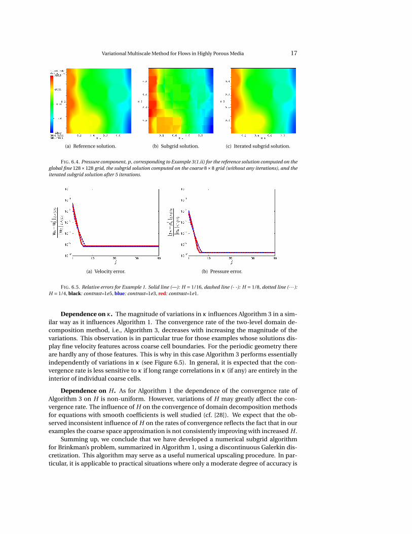
(a) Velocity error. (b) Pressure error.

FIG. 6.5. Relative errors for Example 1. Solid line (—): H = 1/16, dashed line (- -): H = 1/8, dotted line (· · · ):H = 1/4, black: contrast=1e5, blue: contrast=1e3, red: contrast=1e1.

Dependence on κ. The magnitude of variations in κ influences Algorithm 3 in a sim-ilar way as it influences Algorithm 1. The convergence rate of the two-level domain de-composition method, i.e., Algorithm 3, decreases with increasing the magnitude of thevariations. This observation is in particular true for those examples whose solutions dis-play fine velocity features across coarse cell boundaries. For the periodic geometry thereare hardly any of those features. This is why in this case Algorithm 3 performs essentiallyindependently of variations in κ (see Figure 6.5). In general, it is expected that the con-vergence rate is less sensitive to κ if long range correlations in κ (if any) are entirely in theinterior of individual coarse cells.

Dependence on H . As for Algorithm 1 the dependence of the convergence rate ofAlgorithm 3 on H is non-uniform. However, variations of H may greatly affect the con-vergence rate. The influence of H on the convergence of domain decomposition methodsfor equations with smooth coefficients is well studied (cf. [28]). We expect that the ob-served inconsistent influence of H on the rates of convergence reflects the fact that in ourexamples the coarse space approximation is not consistently improving with increased H .

Summing up, we conclude that we have developed a numerical subgrid algorithmfor Brinkman’s problem, summarized in Algorithm 1, using a discontinuous Galerkin dis-cretization. This algorithm may serve as a useful numerical upscaling procedure. In par-ticular, it is applicable to practical situations where only a moderate degree of accuracy is



FIG. 6.6. Relative errors for Example 2. Solid line (—): H = 1/16, dashed line (- -): H = 1/8, dotted line (· · · ):H = 1/4.



required and/or feasible to attain (due to uncertainties in the input data). We have further-more introduced a two-scale iterative domain decomposition algorithm, i.e., Algorithm 3,for solving Darcy’s and Brinkman’s problem. This algorithm is an extension of the subgridAlgorithm 1, and ensures convergence to the solution of the global fine discretization. Thedeveloped algorithms require: (1) the solution of coarse global problem and (2) mutuallyindependent fine local problems. This makes all algorithms very suitable for paralleliza-tion.

Acknowledgments. The research of O. Iliev was supported by DFG Project “Multiscaleanalysis of two-phase flow in porous mediawith complex heterogeneities”. R. Lazarov hasbeen supported by award KUS-C1-016-04, made by KAUST, made by King Abdullah Uni-versity of Science and Technology (KAUST), by NSF Grant DMS-0713829. J. Willems wassupported by DAAD-PPP D/07/10578, NSF Grant DMS-0713829, and the Studienstiftungdes deutschen Volkes (German National Academic Foundation).

The authors express sincere thanks to Dr. Yalchin Efendiev for his valuable commentsand numerous discussion on the subject of this paper.

REFERENCES





FIG. 6.9. First velocity component, u1, corresponding to Example 1(1.ii) for the reference solution (computedon the global fine grid), the subgrid solution (without any iterations), and the iterated subgrid solution after 5iterations.

[1] G. Allaire. Homogenization of the Navier-Stokes equations in open sets perforated with tiny holes. I: Ab-stract framework, a volume distribution of holes. Arch. Ration. Mech. Anal., 113(3):209–259, 1991.

[2] P. Angot. Analysis of singular perturbations on the Brinkman problem for fictitious domain models ofviscous flows. Math. Methods Appl. Sci., 22(16):1395–1412, 1999.

[3] T. Arbogast. Analysis of a two-scale, locally conservative subgrid upscaling for elliptic problems. SIAM J.Numer. Anal., 42(2):576–598, 2004.

[4] T. Arbogast and K. Boyd. Subgrid upscaling and mixed multiscale finite elements. SIAM J. Numer. Anal.,44(3):1150–1171, 2006.

[5] T. Arbogast and H. L. Lehr. Homogenization of a Darcy-Stokes system modeling vuggy porous media.Comput. Geosciences, 10(2):291–302, 2006.

[6] W. Bangerth, R. Hartmann, and G. Kanschat. deal.II – a general purpose object oriented finite elementlibrary. ACM Trans. Math. Softw., 33(4):24/1–24/27, 2007.

[7] J. Bear and Y. Bachmat. Introduction to Modeling of Transport Phenomena in Porous Media. Kluver Ace-demic Publishers, Dordrecht, Netherlands, 1990.

[8] F. Brezzi and M. Fortin. Mixed and Hybrid Finite Element Methods, volume 15 of Springer Series in Compu-tational Mathematics. Springer, 1st edition, 1991.

[9] H. C. Brinkman. A calculation of the viscouse force exerted by a flowing fluid on a dense swarm of particles.Appl. Sci. Res., A1:27–34, 1947.

[10] A. N. Bugrov and S. Smagulov. The fictitious regions method in boundary value problems for Navier-Stokesequations. Mathematical Models of Fluid Flows (Russian), pp. 79 – 90, 1978.

[11] M.A. Christie and M.J. Blunt. Tenth SPE comparative solution project: A comparison of upscaling tech-niques. SPE Res. Eng. Eval., 4:308–317, 2001.

[12] M. Dauge. Elliptic Boundary Value Problems in Corner Domains – Smoothness and Asymptotics ofSolutions.Lecture Notes in Mathematics 1341. Springer-Verlag, Berlin, 1988.



FIG. 6.10. First velocity component, u1, corresponding to Example 2(ii) for the reference solution (computedon the global fine grid), the subgrid solution (without any iterations), and the iterated subgrid solution after 5iterations.



[13] Y. R. Efendiev, J. Galvis, and P. S. Vassilevski. Spectral element agglomerate algebraic multigrid methods forelliptic problems with high-contrast coefficients. Technical Report ISC-09-01, Institute for ScientificComputation, Texas A& M University, 2009.

[14] Y. R. Efendiev, J. Galvis, and X. H. Wu. Multiscale finite element and domain decomposition methods forhigh-contrast problems using local spectral basis functions. Technical Report ISC-09-05, Institute forScientific Computation, Texas A& M University, 2009.

[15] Y. R. Efendiev and T. Hou. Multiscale Finite Element Methods. Theory and Applications. Springer, 2009.[16] R. Glowinski, T-W. Pan, and J. Périaux. A fictitious domain method for external incompressible viscous flow

modeled by Navier-Stokes equations. Comp. Meth. Appl. Mech. Engng., 112:133 – 148, 1994.[17] P. Grisvard. Boundary Value Problems in Non-Smooth Domains. Pitman, London, 1985.[18] A. Hannukainen, M. Juntunen, J. Könnö, and R. Stenberg. Finite element methods for the Brinkman prob-

lem. Talk at Center for Subsurface Modeling Affiliates Meeting, Helsinki University of Technology,October 14–15, 2009.

[19] U. Hornung, editor. Homogenization and Porous Media, volume 6 of Interdisciplinary Applied Mathemat-ics. Springer, 1st edition, 1997.

[20] O. P. Iliev, R. D. Lazarov, and J. Willems. Discontinuous Galerkin subgrid finite element method for approx-imation of heterogeneous Brinkman’s equations. In Large-Scale Scientific Computing, volume 5910 ofLecture Notes in Comput. Sci., pages 14–25. Springer-Verlag, Berlin, Heidelberg, 2010.

[21] W. Jäger and A. Mikelic. On the boundary conditions at the contact interface between a porous mediumand a free fluid. Annali della Scuola Normale Superiore di Pisa, Vol 23:403–465, 1996.

[22] V. V. Jikov, S. M. Kozlov, and O. A. Oleinik. Homogenization of Differential Operators and Integral Function-als. Springer, 1st edition, 1994.

[23] M. Kaviany. Principles of Heat Transfer in Porous Media. Springer-Verlag, New York, 1991.[24] K. Khadra, P. Angot, S. Parneix, and J.-P. Caltagirone. Fictitious domain approach for numerical modelling




of Navier-Stokes equations. International Journal for Numerical Methods in Fluids, 34:651–684, 2000.[25] A. N. Konovalov. The fictitious regions method in problems of mathematical physics. Computing methods

in applied sciences and enginering, Proc. 4th int. Symp., Versailles 1979, pp. 29–40, 1980.[26] W. J. Layton, F. Schieweck, and I. Yotov. Coupling fluid flow with porous media flow. SIAM J. Numer. Anal.,

40(6):2195–2218, 2002.[27] L.-P. Lefebvre, J.B. Banhart, and D.C. Dunand. Porous metals and metallic foams: Current status and recent

developments. Advanced Engineering Materials, 10(9):775–787, 2008.[28] T. P. A. Mathew. Domain Decomposition Methods for the Numerical Solution of Partial Differential Equa-

tions. Lecture Notes in Computational Science and Engineering. Springer, Berlin Heidelberg, 2008.[29] J. Nolen, G. Papanicolaou, and O. Pironneau. A framework for adaptive multiscale methods for elliptic

problems. Multiscale Model. Simul., 7(1):171–196, 2008.[30] J.A. Ochoa-Tapia and S. Whitaker. Momentum transfer at the boundary between a porous medium and a

homogeneous fluid. I. Theoretical development. Int. J. Heat Mass Transfer, 38:2635–2646, 1995.[31] P. Popov, L. Bi, Y. Efendiev, R. Ewing, G. Qin, and J. Li. Multi-physics and multi-scale methods for modeling

fluid flows through naturally fractured vuggy carbonate reservoirs. 15th SPE Middle East Oil & GasShow and Conference, Kingdom of Bahrain, 11-14 March, 2007, 2007. SPE 105378.

[32] K.R. Rajagopal. On a hierarchy of approximate models for flows of incompressible fluids through poroussolids. Math. Models Methods Appl. Sci., 17(2):215–252, 2007.

[33] A.A. Samarskii, P.N. Vabishchevich, O.P. Iliev, and A.G. Churbanov. Numerical simulation of convec-tion/diffusion phase change problems – a review. Int. J. Heat Mass Transfer, 36(17):4095–4106, 1993.

[34] D. Schötzau, Ch. Schwab, and A. Toselli. Mixed hp-DGFEM for incompressible flows. SIAM J. Numer. Anal.,40(6):2171–2194, 2003.

[35] M.V. Twigg and J.T. Richardson. Fundamentals and applications of structured ceramic foam catalysts. Ind.Eng. Chem. Res, 46:4166–4177, 2007.

[36] P. N. Vabishchevich. The method of fictitious domains in problems of mathematical physics. Moscow StateUniversity Publishing House (Russian), 158 pages, Moscow, 1991.

[37] J. Van lent, R. Scheichl, and I. G. Graham. Energy-minimizing coarse spaces for two-level Schwarz methodsfor multiscale PDEs. Numer. Linear Algebra Appl., 16(10):775–799, 2009.

[38] P. S. Vassilevski. General constrained energy minimization interpolation mapping for AMG. Siam J. Sci.Comp., 32:1 – 13, 2010.

[39] J. Wang and X. Ye. New finite element methods in computational fluid dynamics by H(div) elements. SIAMJ. Numer. Anal., 45(3):1269–1286, 2007.

[40] J. Willems. Numerical Upscaling for Multiscale Flow Problems – Analysis and Algorithms. Suedwest-deutscher Verlag fuer Hochschulschriften, 2009.

[41] X. H. Wu, Y. Efendiev, and T. Y. Hou. Analysis of upscaling absolute permeability. Discrete Contin. Dyn.Syst., Ser. B, 2(2):185–204, 2002.

[42] J. C. Xu and L. T. Zikatanov. On an energy minimizing basis for algebraic multigrid methods. Comput. Vis.Sci., 7(3-4):121–127, 2004.

VARIATIONAL MULTISCALE FINITE ELEMENT METHOD FOR … · it is called perturbed Stokes’s system,...

Documents

Transcript of VARIATIONAL MULTISCALE FINITE ELEMENT METHOD FOR … · it is called perturbed Stokes’s system,...