PHYSICAL REVIEW A 82, 023611 (2010)

Variational methods with coupled Gaussian functions for Bose-Einstein condensateswith long-range interactions. II. Applications

Stefan Rau, Jorg Main, Holger Cartarius, Patrick Koberle, and Gunter WunnerInstitut fur Theoretische Physik 1, Universitat Stuttgart, D-70550 Stuttgart, Germany

(Received 28 April 2010; published 13 August 2010)

Bose-Einstein condensates with an attractive 1/r interaction and with dipole-dipole interaction are investigatedin the framework of the Gaussian variational ansatz introduced by S. Rau, J. Main, and G. Wunner [Phys. Rev. A82, 023610 (2010)]. We demonstrate that the method of coupled Gaussian wave packets is a full-fledged alternativeto direct numerical solutions of the Gross-Pitaevskii equation, or even superior in that coupled Gaussians arecapable of producing both stable and unstable states of the Gross-Pitaevskii equation and thus of giving access toyet unexplored regions of the space of solutions of the Gross-Pitaevskii equation. As an alternative to numericalsolutions of the Bogoliubov–de Gennes equations, the stability of the stationary condensate wave functions isinvestigated by analyzing the stability properties of the dynamical equations of motion for the Gaussian variationalparameters in the local vicinity of the stationary fixed points. For blood-cell-shaped dipolar condensates it isshown that on the route to collapse the condensate passes through a pitchfork bifurcation, where the ground stateitself turns unstable, before it finally vanishes in a tangent bifurcation.

DOI: 10.1103/PhysRevA.82.023611 PACS number(s): 67.85.−d, 03.75.Hh, 05.30.Jp, 05.45.−a

I. INTRODUCTION

In the previous article [1] variational methods withcoupled Gaussian functions for Bose-Einstein condensateswith long-range interactions were developed. The purposeof this article is to demonstrate the power of this ap-proach by applying the variational methods to two dif-ferent types of condensates, viz., a monopolar condensatewith an attractive gravitylike 1/r interaction and a dipolarcondensate.

Monopolar condensates with an attractive 1/r interaction,originally proposed by O’Dell et al. [2], have unique stabilityproperties. For a wide range of the scattering length thecondensate is stable without an external trap. Additionally,the gravitylike interaction of a monopolar condensate maybe an opportunity to investigate usually large-scale physicalproperties like, for example, boson stars [3] at a laboratoryscale. The “monopolar” interaction of two neutral atomswith positions r and r ′ is induced by the presence ofexternal electromagnetic radiation. O’Dell et al. [2] suggestsix triads of orthogonal laser beams to induce the interatomicpotential Wlr(r,r ′) = −u/|r − r ′|, where u depends on theintensity and wave vector of the radiation and on the isotropicpolarizability of the atoms. Although this system has notyet been realized experimentally, it has already served as amodel to compare results obtained analytically and with exactnumerical techniques [4–6].

By contrast, Bose-Einstein condensates with a long-rangedipole-dipole interaction Wlr(r,r ′) ∼ (1 − 3 cos2 θ )|r − r ′|−3

have been obtained experimentally with 52Cr atoms in 2005by Griesmaier et al. [7,8], and more recently in 2008 byBeaufils et al. [9]. The collapse of the condensate alsohas been subject to extensive experimental studies [10].Theoretical investigations have so far mostly been based onlattice simulations [11–13] or on a simple variational approachwith a Gaussian-type orbital [14]. For a review on dipolarcondensates, see [15].

In this article we extend and elaborate in more detailpreliminary work presented in [16]. In Sec. II the results

for the monopolar condensates are presented and discussed.It is shown that only three to five coupled Gaussians aresufficient to achieve convergence of the mean-field energy,the chemical potential, and the lowest eigenvalues of thestability matrix. In Sec. III the method of coupled Gaussiansis applied to dipolar Bose-Einstein condensates (BECs) toclarify the theoretical nature of the collapse mechanism ofblood-cell-shaped condensates. On the route to collapse thecondensates pass through a pitchfork bifurcation, where theground state itself turns unstable, before it finally vanishes ina tangent bifurcation. Conclusions are drawn in Sec. IV.

II. MONOPOLAR CONDENSATES

The time-independent Gross-Pitaevskii equation (GPE) fora self-trapped condensate with a short-range contact inter-action with scattering length a and a long-range monopolarinteraction reads[

−� + 8πNa

au

|ψ(r)|2 − 2N

∫d3r ′ |ψ(r ′)|2

|r − r ′|]ψ(r)

= µψ(r), (1)

where the natural “atomic” units introduced in Ref. [4] wereused. Lengths are measured in units of a “Bohr radius”au = h2/(mu), energies in units of a “Rydberg energy”Eu = h2/(2ma2

u), and times in units of tu = h/Eu, where u

determines the strength of the atom-atom interaction [2] andm is the mass of one boson. The number of bosons N canbe eliminated from Eq. (1) by using scaling properties of thesystem [4,6]. We define r = r/N , ψ = N3/2ψ , which leavesthe norm of the wave function invariant, asc = N2a/au, µ =µ/N2, omit the tilde in what follows, substitute µ → i(d/dt),and finally obtain the time-dependent GPE in scaled “atomic”units:[

−� + 8πasc |ψ(r,t)|2 − 2∫

d3r ′ |ψ(r ′,t)|2|r − r ′|

]ψ(r,t)

= id

dtψ(r,t). (2)

1050-2947/2010/82(2)/023611(13) 023611-1 ©2010 The American Physical Society

RAU, MAIN, CARTARIUS, KOBERLE, AND WUNNER PHYSICAL REVIEW A 82, 023611 (2010)

It is known that for Bose-Einstein condensates with attractive1/r interaction two real radially symmetric solutions, theground state and a collectively excited state, exist. By varyingthe scattering length asc, they are created in a tangentbifurcation at a critical value of asc [4–6]. Below the tangentbifurcation no stationary solutions exist. Approaching thebifurcation point from higher scattering lengths the condensatecollapses. A similar behavior is found for dipolar condensates[14] and condensates without long-range interactions [17].

For the monopolar GPE numerically exact solutions exist.The numerical procedure for the direct integration of the GPEis introduced in Refs. [4–6]. It is our purpose to investigatethe two states connected via the tangent bifurcation with thecoupled Gaussian wave packet method. We use the ansatz

ψ(r) =N∑

k=1

ei(akr2+γ k ) =N∑

k=1

gk (3)

for condensates with spherical symmetry. Following theprocedure outlined in [1], the dynamical equations for thevariational parameters read

γ k = 6iak − vk0, (4a)

ak = −4(ak)2 − 12V k

2 , (4b)

for k = 1, . . . ,N . The quantities vk0 and V k

2 are obtained fromthe (2N × 2N )-dimensional linear set of equations (k,l =1, . . . ,N )(

(1)kl (r2)kl

(r2)lk (r4)kl

) (vk

012V k

2

)=

N∑k=1

(〈gl|Veff|gk〉〈gl|r2Veff|gk〉

), (5)

where Veff = Vsc + Vm is the sum of the contact and monopolarpotential, and the matrix elements read

(1)lk : 〈gl|gk〉 = π3/2 eiγ kl

(−iakl)3/2, (6a)

(r2)lk : 〈gl|r2|gk〉 = 3

2π3/2 eiγ kl

(−iakl)5/2, (6b)

(r4)lk : 〈gl|r4|gk〉 = 15

4π3/2 eiγ kl

(−iakl)7/2, (6c)

〈gl|Vsc|gk〉 =N∑

i,j=1

8ascπ5/2 eiγ klij

(−iaklij )3/2, (6d)

〈gl|Vm|gk〉 = 4N∑

i,j=1

π5/2 eiγ klij

aij akl√−iaklij

, (6e)

〈gl|r2Vsc|gk〉 = 12N∑

i,j=1

ascπ5/2 eiγ klij

(−iaklij )5/2, (6f)

〈gl|r2Vm|gk〉 = 2N∑

i,j=1

π5/2 eiγ klij

(2aij + 3akl)

aij (akl)2(−iaklij )3/2, (6g)

with the abbreviations

akl = ak − (al)∗, aij = ai − (aj )∗, (7a)

γ kl = γ k − (γ l)∗, γ ij = γ i − (γ j )∗, (7b)

aklij = akl + aij , γ klij = γ kl + γ ij . (7c)

A. Stationary solutions

Stationary solutions of the GPE can be computed viaa nonlinear root search of the dynamical equations (4) asoutlined in [1]. The Gaussian parameters obtained from theroot search are then used to calculate the mean-field energy,

Emf =N∑

k,l=1

2π3/2eiγ kl

[−3

ak(al)∗

(akl)2√−iakl

+N∑

i,j=1

πeiγ ij

√−iaklij

×(

2asc

−iaklij+ 1

aij akl

)], (8)

and the chemical potential,

µ =N∑

k,l=1

2π3/2eiγ kl

[−3

ak(al)∗

(akl)2√−iakl

+N∑

i,j=1

πeiγ ij

√−iaklij

×(

4asc

−iaklij+ 2

aij akl

)]. (9)

For the variational ansatz with only one single Gaussianfunction (N = 1) the results can be obtained analytically [5,6],viz.,

EN=1mf = − 4

9π

1 ± 2√

1 + 8asc3π(

1 ±√

1 + 8asc3π

)2(10)

for the mean field energy, and

µN=1 = − 4

9π

5 ± 4√

1 + 8asc3π(

1 ±√

1 + 8asc3π

)2(11)

for the chemical potential.The results of the variational computations with N = 1 to

N = 5 coupled Gaussian functions are presented in Fig. 1(a)for the mean-field energy and in (b) for the chemical potential.For comparison, the results of the exact solution obtainedby direct numerical integration of the GPE are shown asred triangles. Although the variational solution with a singleGaussian significantly differs from the exact calculation, thequalitative behavior is the same: Two solutions emerge in atangent bifurcation at a critical scattering length, which isacr,v

sc = −3π/8 = −1.178 097 and acr,nsc = −1.025 147 for the

variational and exact calculation, respectively [4]. Note thatthe excited state with higher mean-field energy has a lowerchemical potential than the ground state.

The main purpose of Fig. 1 is to demonstrate howthe coupling of only N = 2 to N = 5 Gaussian functionsdrastically improves the results obtained with a simpleGaussian-type orbital. The coupling of only two Gaussianfunctions already leads to a significant improvement for boththe mean field energy value and the chemical potential.For three or more coupled Gaussians, the results in Fig. 1can no longer be distinguished from the numerically exactsolution. The enlargements in Fig. 1 illustrate the rapid con-vergence of the results with increasing number N of coupledGaussians.

Detailed values for the mean-field energy and the chemicalpotential of the ground state and the excited state at scattering

023611-2

VARIATIONAL METHODS WITH . . . . II. APPLICATIONS PHYSICAL REVIEW A 82, 023611 (2010)

-2

-1.6

-1.2

-0.8

-1.15 -1.1 -1.05 -1 -0.95 -0.9 -0.85

µ

asc

(b)N = 1N = 2N = 3N = 4N = 5exact

-0.8

-0.7

-0.6

-1.03 -1.02

-0.14

-0.1

-0.06

-0.02

-1.1 -1 -0.9 -0.8 -0.7 -0.6

Em

f

asc

(a)N = 1N = 2N = 3N = 4N = 5exact

-0.143

-0.142

-1.03 -1.02

FIG. 1. (Color online) (a) Mean-field energy Emf for self-trappedcondensates with attractive 1/r interaction as a function of thescattering length obtained by using up to five coupled Gaussian wavepackets (N = 1, . . . ,5, respectively) in comparison with the resultof the accurate numerical solution of the stationary GPE (exact). (b)Same as (a) but for the chemical potential µ.

length asc = −1 close to the tangent bifurcation are presentedin Table I. The coupling of three Gaussian functions alreadyyields an accuracy of more than four digits for the mean-fieldenergy of the ground state. Using up to five Gaussians, we cansafely assume the variational result as to be fully convergedto the exact numerical computation marked as N = ∞. Therapid convergence of the critical scattering length acr

sc with

TABLE I. Dependence of the critical scattering length acrsc of

the tangent bifurcation and the mean-field energy and the chemicalpotential of the ground state (g) and the excited state (e) at scatteringlength asc = −1 on the number N of coupled Gaussian functions.

N acrsc E

gmf µg Ee

mf µe

1 −1.178 097 −0.130 383 −0.480 807 −0.084 219 −1.304 5922 −1.032 780 −0.140 151 −0.584 799 −0.136 826 −0.892 3763 −1.025 527 −0.140 637 −0.595 154 −0.138 380 −0.862 5624 −1.025 167 −0.140 655 −0.595 659 −0.138 449 −0.860 8625 −1.025 149 −0.140 656 −0.595 682 −0.138 452 −0.860 767∞ −1.025 147 −0.140 657 −0.595 685 −0.138 453 −0.860 757

0

0.05

0.1

0.15

0.2

0.25

0.3

0.35

0 1 2 3 4 5 6 7 8

ψ

r

(b)

N = 1N = 2N = 3N = 4N = 5exact

0.256

0.258

0.26

0 0.05 0.1 0.15

0

0.02

0.04

0.06

0.08

0.1

0.12

0.14

0.16

0 1 2 3 4 5 6 7 8

ψ

r

(a)

N = 1N = 2N = 3N = 4N = 5exact

0.156

0.157

0.158

0.159

0 0.05 0.1 0.15

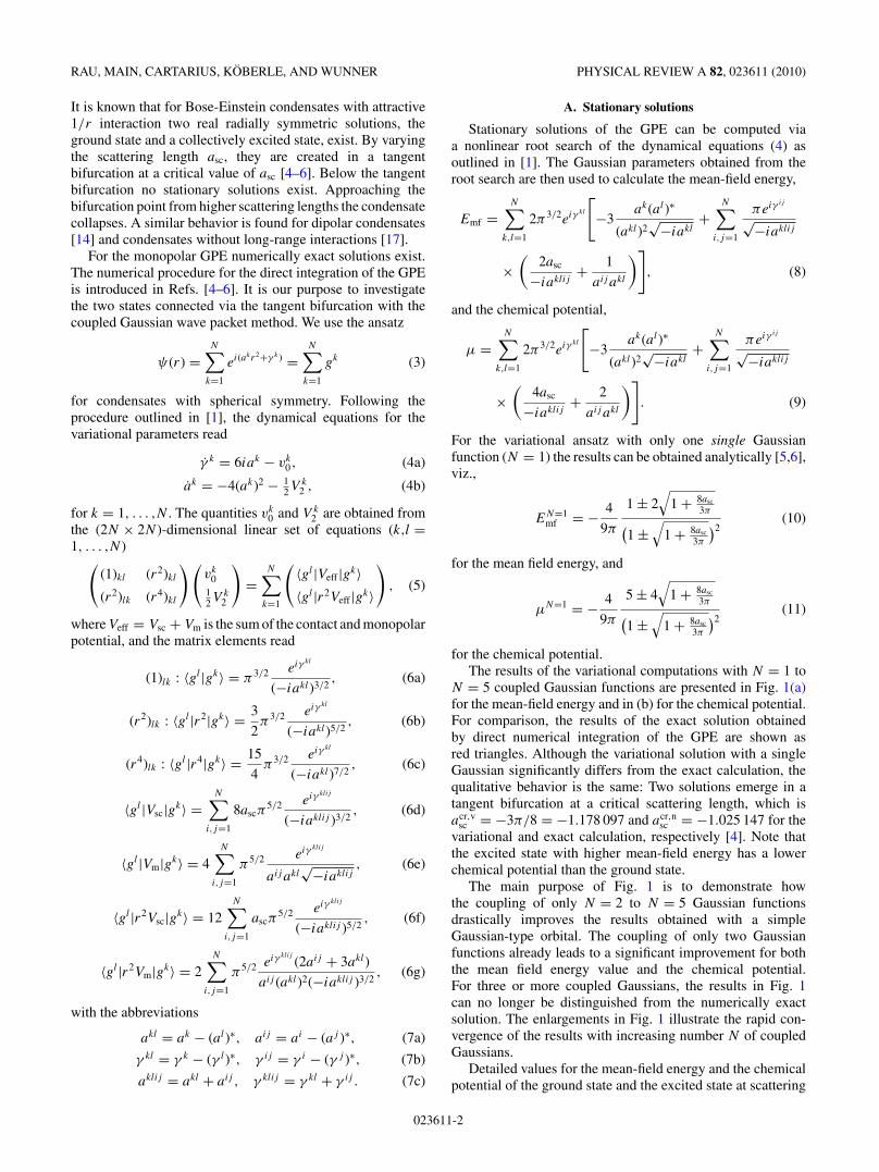
FIG. 2. (Color online) Wave function ψ(r) of (a) the stable groundstate and (b) the excited state at scattering length asc = −1 close to theexact numerical bifurcation. The calculations with coupled Gaussiansconverge rapidly to the exact numerical wave function (triangles).

increasing number of coupled Gaussians is also illustrated inTable I.

In previous work [4] it has been noted that the peakamplitude of the exact wave function at the center r =0 is poorly reproduced by a Gaussian-type orbital. Here,we illustrate that superpositions of Gaussian functions canaccurately approximate the exact wave function and thus alsoprovide the correct peak amplitude.

In Fig. 2 we choose the scattering length asc = −1 close tothe exact numerical bifurcation at acr

sc = −1.025 15 to comparethe wave function of the variational and the numerically exactground and excited state. As a second example, we chooseasc = −0.6 in Fig. 3, which lies farther away from the criticalscattering length. The rapid convergence of the variationalwave functions with the number of Gaussians increasing fromN = 1 to 5 is impressive, as can be seen in the insets in Figs. 2and 3. Note that far from the bifurcation the wave function ofthe stable state in Fig. 3(a) and the wave function of the excitedstate in Fig. 3(b) differ greatly, while for asc = −1 both wavefunctions in Figs. 2(a) and 2(b) are similar. At the tangentbifurcation, both merging states, the stable ground state andthe excited state, are described by the same wave function. The

023611-3

RAU, MAIN, CARTARIUS, KOBERLE, AND WUNNER PHYSICAL REVIEW A 82, 023611 (2010)

0

0.2

0.4

0.6

0.8

1

0 2 4 6 8 10

ψ

r

(b)

N = 1N = 2N = 3N = 4N = 5exact

0.85

0.9

0.95

1

1.05

0 0.1 0.2

0

0.02

0.04

0.06

0.08

0.1

0 2 4 6 8 10

ψ

r

(a)

N = 1N = 2N = 3N = 4N = 5exact

0.088

0.089

0.09

0.091

0 0.05 0.1 0.15

FIG. 3. (Color online) Same as Fig. 2 but at scattering lengthasc = −0.6.

reason is that due to the nonlinearity of the GPE, the solutionat the tangent bifurcation has the properties of an “exceptionalpoint” [5].

Figures 2 and 3 apparently show that the form of theexact numerical wave function differs from the simple N = 1Gaussian form. The inclusion of five Gaussians, however,achieves excellent results. Therefore, we can assume thevariational ansatz using five coupled Gaussian functions tobe converged with sufficient accuracy to calculate all majorproperties of the system.

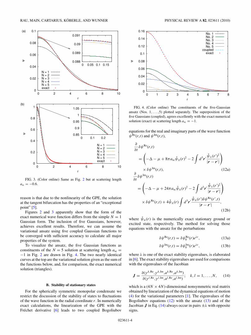
To visualize the ansatz, the five Gaussian functions asconstituents of the N = 5 solution at scattering length asc =−1 in Fig. 2 are drawn in Fig. 4. The two nearly identicalcurves at the top are the variational solution given as the sum ofthe functions below, and, for comparison, the exact numericalsolution (triangles).

B. Stability of stationary states

For the spherically symmetric monopolar condensate werestrict the discussion of the stability of states to fluctuationsof the wave function in the radial coordinate r . In numericallyexact calculations, the linearization of the GPE with theFrechet derivative [6] leads to two coupled Bogoliubov

0

0.02

0.04

0.06

0.08

0.1

0.12

0.14

0.16

0 1 2 3 4 5 6 7 8

ψ

r

No. 1No. 2No. 3No. 4No. 5

coupledexact

FIG. 4. (Color online) The constituents of the five-Gaussianansatz (Nos. 1, . . . ,5) plotted separately. The superposition of thefive Gaussians (coupled), agrees excellently with the exact numericalsolution (exact) at scattering length asc = −1.

equations for the real and imaginary parts of the wave functionψRe(r,t) and ψ Im(r,t),

∂

∂tδψRe(r,t)

=(

−� − µ + 8πascψ±(r)2 − 2∫

d3r ′ ψ±(r ′)2

|r − r ′|

)

× δψ Im(r,t), (12a)∂

∂tδψ Im(r,t)

=(

−� − µ + 24πascψ±(r)2 − 2∫

d3r ′ ψ±(r ′)2

|r − r ′|

)

× δψRe(r,t) + 4ψ±(r)∫

d3r ′ ψ±(r ′)δψRe(r ′,t)|r − r ′| ,

(12b)

where ψ±(r) is the numerically exact stationary ground orexcited state, respectively. The method for solving thoseequations with the ansatz for the perturbations

δψRe(r,t) = δψRe0 (r)eλt , (13a)

δψ Im(r,t) = δψ Im0 (r)eλt , (13b)

where λ is one of the exact stability eigenvalues, is elaboratedin [6]. The exact stability eigenvalues are used for comparisonswith the eigenvalues of the Jacobian

J = ∂(γ k,Re,γ k,Im,ak,Re,ak,Im)

∂(γ l,Re,γ l,Im,al,Re,al,Im); k, l = 1, . . . ,N, (14)

which is a (4N × 4N )-dimensional nonsymmetric real matrixobtained by linearization of the dynamical equations of motion(4) for the variational parameters [1]. The eigenvalues of theBogoliubov equations (12) with the ansatz (13) and of theJacobian J in Eq. (14) always occur in pairs ±λ with oppositesigns.

023611-4

VARIATIONAL METHODS WITH . . . . II. APPLICATIONS PHYSICAL REVIEW A 82, 023611 (2010)

1. First pair of stability eigenvalues

For the ansatz with a single Gaussian there is, afterexploiting the normalization condition, only one variationalparameter a = a1 in Eq. (3) for the (complex) width of theGaussian function, and the eigenvalues of the Jacobian canbe calculated analytically [6,18]. For the ground state the twoeigenvalues

λg± = ±16i

9π

4

√1 + 8asc

3π(√1 + 8asc

3π+ 1

)2(15)

are purely imaginary for all scattering lengths above the criticalvalue of the tangent bifurcation. For the excited state there aretwo purely real eigenvalues:

λe± = ± 16

9π

4

√1 + 8asc

3π(√1 + 8asc

3π− 1

)2. (16)

For N � 2 coupled Gaussian functions the Jacobian J isdiagonalized numerically. The stability eigenvalues obtainedwith a single Gaussian function [Eqs. (15) and (16)], thecorresponding pair of eigenvalues of the Jacobian J for N = 2to N = 5 coupled Gaussians, and the corresponding pair ofthe exact eigenvalues are presented in Fig. 5. Similar to thecalculation of the mean-field energy and chemical potential,the pair of eigenvalues merges and vanishes at a tangentbifurcation. As we include more Gaussian functions, thecritical scattering length shifts to higher values and convergesto the bifurcation of the exact numerical solution, as wasexpected from the behavior of the energies. Figure 5(a) showsthe first pair of eigenvalues of the stable ground state. They arepurely imaginary. Since this is true for all stability eigenvaluesof the ground state (see below), the branch of the ground state isstable. Figure 5(b) shows the first eigenvalue pair of the excitedstate. These eigenvalues are purely real, and thus the excitedstate is unstable. The tangent bifurcation is clearly exhibitedfor both states, as each pair of eigenvalues ±λ merges at zeroand vanishes at the critical scattering length.

It is important to note that similar to the convergenceproperties of the mean-field energy and the chemical po-tential, very few coupled Gaussians are already sufficient toachieve excellent results for the lowest stability eigenvalues.Results obtained with N � 3 coupled Gaussians cannot bedistinguished in Fig. 5 from the numerically exact values.

2. Additional pairs of stability eigenvalues

In contrast to the calculation with a single Gaussian,which can provide only one pair of eigenvalues, additionaleigenvalues are accessible when using coupled Gaussian wavefunctions. We compare them with the exact stability eigen-values in Fig. 6. The additional eigenvalues are increasinglydifficult to obtain in the numerically exact computation. In thefollowing, we refer to the eigenvalues with the second-lowestabsolute value simply as “second (pair of)” eigenvalues, etc.Numerically exact data is available for the lowest three pairsof eigenvalues of the stable ground state, and therefore herewe compare the variational solution only with the lowest threeeigenvalues of the stable solution.

-2

-1.5

-1

-0.5

0

0.5

-1.2 -1.15 -1.1 -1.05 -1 -0.95 -0.9 -0.85 -0.8

Imλ

asc

(a)

stable, 1st pair

Im λ 1Im λ 2Im λ 3Im λ 4Im λ 5exact

-0.1

0

0.1

-1.04 -1.03 -1.02

-1.5

-1

-0.5

0

0.5

1

1.5

-1.2 -1.15 -1.1 -1.05 -1 -0.95 -0.9 -0.85 -0.8

Re

λ

asc

(b)

unstable, 1st pair

Re λ 1Re λ 2Re λ 3Re λ 4Re λ 5exact

-0.1

0

0.1

-1.03 -1.02

FIG. 5. (Color online) First pair of eigenvalues as a function of thescattering length for an increasing number of coupled Gaussians andfor the exact numerical calculation. (a) The two lowest eigenvaluesof the stable ground state are purely imaginary. (b) The unstableexcited state with a pair of purely real eigenvalues. Vanishing realor imaginary parts are not shown. The insets illustrate the rapidconvergence of the variationally computed eigenvalues to the exactsolutions of the Bogoliubov equations.

Figure 6(a) shows the second pair of eigenvalues for thestable ground state and the unstable excited state. The secondpairs of eigenvalues are all purely imaginary and converge withincreasing number of coupled Gaussians to the numericallyexact eigenvalues.

The third pair of eigenvalues presented in Fig. 6(b) isqualitatively similar to the second pair. For any number ofcoupled Gaussians, they are purely imaginary. Figures 6(a)and 6(b) suggest that as the number of the eigenvalue rises,the convergence progresses more slowly. However, using fiveGaussians in Fig. 6(b) even the third pair of the variationaleigenvalues shows no apparent deviation from the numericallyexact result.

3. Variations of the ground-state wave function

We investigated the stability of the stationary states bylinearizing the dynamical equations in the vicinity of thefixed points. For the stable ground state there are only purelyimaginary eigenvalues; for the unstable excited state we foundone pair of real eigenvalues. In addition to the analysis of

023611-5

RAU, MAIN, CARTARIUS, KOBERLE, AND WUNNER PHYSICAL REVIEW A 82, 023611 (2010)

-3

-2

-1

0

1

2

3

-1.05 -1 -0.95 -0.9 -0.85 -0.8 -0.75 -0.7 -0.65 -0.6

Imλ

asc

(b)N = 2N = 3N = 4N = 5exact

-2

-1.5

-1

-0.5

0

0.5

1

1.5

2

-1.05 -1 -0.95 -0.9 -0.85 -0.8 -0.75 -0.7 -0.65 -0.6

Imλ

asc

(a)N = 2N = 3N = 4N = 5exact

FIG. 6. (Color online) (a) Second pair of eigenvalues as a functionof the scattering length for varying number of coupled Gaussians andfor the exact numerical calculation for the stable ground state and theunstable excited state. Numerically exact eigenvalues (triangles) areonly available for the stable ground state. All eigenvalues are purelyimaginary; vanishing real parts are not shown. (b) Same as (a) but forthe third pair of eigenvalues.

the eigenvalues λi of the Jacobian of the linearized dynamicalequations, we can evaluate the respective eigenvectors, whichprovide the form of the wave function’s fluctuations.

We focus on variations of the Gaussian parameters cor-responding to the eigenvector i and calculate the first-orderpower series of the wave function ψ(r,t) at the fixed point(FP) [1],

δψi(r,t) =N∑

k=1

(ir2δa

k,Rei − r2δa

k,Imi + iδγ

k,Rei − δγ

k,Imi

)× gk|FP(r)eλi t . (17)

For a scattering length of asc = −0.8, Fig. 7 shows thevariation of the ground-state wave function for the eigenvectorscorresponding to the first (a), second (b), and third (c) pair ofeigenvalues ±λ for the variational calculation, as well as forthe numerically exact calculation.

In Fig. 7(a) the variation of the wave function δψ convergesrapidly with increasing number of Gaussian functions to thenumerical solution. For the second and third pair of eigenvalues

-0.6

-0.4

-0.2

0

0.2

0.4

0.6

0.8

1

0 2 4 6 8 10 12 14

δΨ

r

(b)N = 2N = 5

numerical

-0.4

-0.2

0

0.2

0.4

0.6

0.8

1

0 2 4 6 8 10 12 14

δΨ

r

(c)N = 2N = 5

numerical

-0.5

0

0.5

1

1.5

2

2.5

3

3.5

4

4.5

0 2 4 6 8 10 12 14

δΨ

r

(a)N = 2N = 3N = 4N = 5

numerical

FIG. 7. (Color online) Deviations of the ground-state wavefunction according to the eigenvectors of the (a) first, (b) second, and(c) third pair of eigenvalues ±λ of the stability analysis at scatteringlength asc = −0.8.

in Figs. 7(b) and 7(c), the variation using five Gaussians isalmost identical to the numerical variation. For the higherpairs of eigenvalues, the solution obviously converges slower.However, we note that it also becomes more and more difficultto obtain the exact solutions. The spatial extension of thefluctuations δψ exceeds the elongation of the wave functionψ (cf. Figs. 2 and 3) by far and it becomes hard to achieve

023611-6

VARIATIONAL METHODS WITH . . . . II. APPLICATIONS PHYSICAL REVIEW A 82, 023611 (2010)

converged fluctuations. The differences between the numericaland the N = 5 solution in Fig. 7(c) can already be explainedby the quality of the numerical approach.

III. DIPOLAR CONDENSATES

The stationary GPE for a dipolar BEC with a harmonic trap,the short-range s-wave scattering term, and the long-rangedipolar interaction reads

[−� + γ 2

x x2 + γ 2y y2 + γ 2

z z2 + 8πNa

ad

|ψ(r)|2

+N

∫d3r ′ 1 − 3 cos2 θ

|r − r ′|3 |ψ(r ′)|2]ψ(r) = µψ(r). (18)

In Eq. (18) the “natural units” for this system introduced in[14] have been used, which are h for action, md = 2m formass, ad = mdµ0µ

2/(4πh2) for length, Ed = h2/(mda2d ) for

energy, and ωd = Ed/h for frequency. The angle between theexternal magnetic field in the z direction and the vector r − r ′is denoted θ , and N is the particle number. As in [14] we scaler = N r , ψ = N−3/2ψ , insert the newly defined quantities inEq. (18), redefine γi = N2γi , µ = N2µ, and afterward omitthe tilde once again. With the replacement µ → i(d/dt) wefinally obtain the time-dependent GPE for a dipolar BEC inparticle-number-scaled dimensionless units,

[−� + γ 2

x x2 + γ 2y y2 + γ 2

z z2 + 8πasc |ψ(r)|2

+∫

d3r ′ 1 − 3 cos2 θ

|r − r ′|3 |ψ(r ′)|2]ψ(r) = i

d

dtψ(r), (19)

with the trap frequencies γx,y,z = N2ωx,y,z/(2ωd ) and thes-wave scattering length asc = a/ad . For dipolar condensatesit is possible to solve the GPE fully numerically on a two-or three-dimensional lattice [12,15]. Ronen et al. [11] andDutta et al. [19] have shown that in certain regions of theparameter space dipolar condensates assume a non-Gaussian,biconcave, “blood-cell-like” shape. In this article we want toapply the variational method with coupled Gaussian functionsintroduced in the preceding article [1]. We show that thevariational technique is a full-fledged alternative to the numer-ical simulations on grids and additionally uncovers unstablestationary solutions not accessible in previous full-numericalevaluations.

The frequency and symmetry of the magnetic trap stronglyinfluences the physical behavior of dipolar Bose-Einsteincondensates. In the following we will analyze one distinct trapsymmetry in detail, where the condensate has a blood-cell-shaped form. The ansatz with coupled Gaussians has provedto be capable of modifying the simple Gaussian form of thewave function for monopolar condensates (see Sec. II A). Thebiconcave shape, however, where the maximum density is nolonger located at the origin is even a stronger challenge for thevariational approach. We investigate the dipolar condensatefor an axially symmetric trap with trap frequencies,

γx = γy ≡ γ = 3600, γz = 25 200,

which is equivalent to the frequency ratio and mean

λ = γz

γ

= 7, γ = 3

√γ 2

γz = 688 7,

and corresponds to a value of D = √γ/2 = 30 in [11].

The trapping frequency in the z direction parallel to theorientation of the dipoles is seven times larger than in theplane perpendicular to that direction, and for some parametersasc the ground state of the condensate has a biconcave, blood-cell-shaped form [11]. In contrast to monopolar condensateswhere the inclusion of additional Gaussian functions providesan improved numerical accuracy of the results, dipolar con-densates offer a wealth of new phenomena with increasingnumber of coupled Gaussian functions, as is shown below.

A. Variational calculations with one and two Gaussian functions

As ansatz for the variational calculations we use the wavefunction

ψ(r,t) =N∑

k=1

ei(akxx2+ak

yy2+akz z2+γ k) ≡

N∑k=1

gk, (20)

where N is the number of coupled Gaussians. For anaxisymmetric trap the stationary solutions are also symmetric;that is, ak

x = aky ≡ ak

. Nevertheless, all stability propertieshave been computed with the fully three-dimensional ansatz.The case of a single Gaussian function (N = 1) has beendiscussed in [14]. In this section we demonstrate that resultsespecially for the mean-field energy and chemical potentialare already substantially improved with the use of only N = 2coupled Gaussians. Results of variational calculations with asingle Gaussian function and numerical simulations on gridsare employed for comparison and discussion.

1. Stationary solutions

Using the variational ansatz (20), stationary solutions ofthe GPE for dipolar BEC are obtained by a numerical rootsearch for the fixed points of the dynamical equations for thevariational parameters as described in detail in the precedingarticle [1].

Figure 8 presents in (a) the mean-field energy and in(b) the chemical potential for the two stationary solutionsobtained with a single Gaussian function and with two coupledGaussians. For the ground state, results of a numerical latticecalculation are also marked in Fig. 8. The numerical simulationwas performed on a lattice with a grid size of 128 × 512 pointsusing fast-Fourier techniques and imaginary time evolution ofan initial wave function.

The variational calculations with one Gaussian (N = 1)show the following behavior. For scattering lengths belowacr,var

sc = −0.037 891 7, there is no stable condensate. Similaras in monopolar condensates two solutions are born at thecritical scattering length in a tangent bifurcation, the stableground state (v1) and an unstable excited state (v2). For adetailed stability analysis, see Sec. III A2. The unstable branchvanishes at scattering length asc = 1/6.

The variational ansatz with N = 1 is limited to the Gaussianshape of the wave function with two width parameters a andaz, and thus the values obtained for the mean-field energy and

023611-7

RAU, MAIN, CARTARIUS, KOBERLE, AND WUNNER PHYSICAL REVIEW A 82, 023611 (2010)

50000

60000

70000

80000

90000

100000

-0.1 0 0.1 0.2 0.3 0.4 0.5

Em

f

asc

(a)v1: N = 1v2: N = 1v1: N = 2v2: N = 2

n1

70000

80000

90000

100000

110000

120000

130000

-0.1 0 0.1 0.2 0.3 0.4 0.5

µ

asc

(b)

v1: N = 1v2: N = 1v1: N = 2v2: N = 2

n1

FIG. 8. (Color online) (a) Mean-field energy and (b) chemicalpotential as a function of the scattering length, variational solution(v) using two Gaussians compared with an exact full-numerical latticecalculation (n1). For two Gaussians (N = 2), the ground state (v1)and the excited state (v2) emerge in a tangent bifurcation at asc =−0.034 202. The unstable branch of the chemical potential in (b) hasa maximum at µmax ≈ 170 000 (not shown) and then vanishes as anearly vertical line at asc = 1/6.

chemical potential are not very accurate. However, the resultsare substantially improved when using a variational ansatz withtwo coupled Gaussians. This can be seen in Fig. 8 especiallyfor the ground state when comparing the N = 2 variationalcomputation with the lattice computation (n1) marked by thetriangles in Fig. 8.

In the full-numerical grid calculations only the groundstate can be obtained. Starting with positive scattering lengthsand decreasing asc, the numerical grid calculations providea ground state down to a critical point acr,num

sc = −0.008.Note that the ground state of the solution using two coupledGaussian wave functions is nearly indistinguishable fromthe numerical lattice calculation in Figs. 8(a) and 8(b). Animportant advantage of the variational method is that it canprovide both stable and unstable states. As is shown in whatfollows, the stability properties of the variational solutions canclarify the mechanism of how the condensate turns unstable.

Regarding the wave functions, one single Gaussian canevidently not adequately represent a blood-cell-shaped con-densate. Two Gaussians not only significantly increase theaccuracy of the mean-field energy, but also greatly improve

the form of the wave function. Even the biconcave shape ofthe dipolar condensate is qualitatively visible in the variationalsolution with two Gaussians, however, the result is not fullyconverged. Exact wave functions are compared in Sec. III Bwith variational results obtained with more than two coupledGaussians.

2. Stability analysis

To perform a stability analysis with numerical latticecalculations, the Bogoliubov–de Gennes equations have to besolved [12,20]. Here we restrict our discussion to the stabilityanalysis of the variational solutions, which is instructiveconsidering nonlinear dynamics and bifurcation theory.

We follow the procedure outlined in [1] and start with thestationary solutions of the GPE calculated using one and twoGaussians. These solutions are fixed points of the dynamicalequations for the Gaussian parameters. We then linearize thesedynamical equations in the vicinity of the fixed point andcalculate the eigenvalues of the Jacobian (see [1]).

The eigenvalues of the ground state obtained with oneGaussian wave function are purely imaginary [see the thingreen lines in Fig. 9(a)]. Therefore, this state is stable. If weperturb the variational parameters of the fixed-point solution,the quasiperiodic motion is confined to the vicinity of thefixed point. Figure 9(b) shows the characteristic eigenvaluesof the unstable excited state. Contrary to the stable state,there are eigenvalues with nonvanishing real parts Re λ,indicated by thick red lines. Perturbations in the direction of thecorresponding eigenvector lead to an exponential growth of theperturbation. Therefore, this state is unstable. Both branchesexist for scattering lengths down to acr

sc = −0.037 891 7, wherethey merge in a tangent bifurcation (see Fig. 8). The tangentbifurcation is apparent in the eigenvalues in Figs. 9(a) and 9(b).

Some eigenvalues of the Jacobian using a wave functionof two coupled Gaussians in Fig. 10 qualitatively agree withthe one-Gaussian calculation. There is one stable groundstate with purely imaginary eigenvalues in Fig. 10(a) andone unstable excited state in Fig. 10(b). However, the two-Gaussian calculation yields additional eigenvalues which arenot available within the limited parameter space of the simpleone-Gaussian calculation. The real and imaginary eigenvaluesare drawn with thick red and thin green lines in Figs. 9 and 10,respectively.

The unstable branches of both calculations in Figs. 9(b)and 10(b), exhibit that for the given parameters of the trapin dipolar condensates, the stability scenario is quite morecomplex than for monopolar condensates. As we can see,there is not only one single pair of imaginary eigenvaluesof the stable solution approaching zero and merging with onepair of real unstable eigenvalues [denoted 1 in Fig. 9(b)] fromthe excited state. For monopolar condensates this real pair ofeigenvalues of the unstable solution remains the only one forincreasing scattering lengths (see Sec. II B). By contrast, here,a second pair of eigenvalues [denoted 2 in Fig. 9(b)] indicatinginstability additionally forms as we follow the excited statefrom the bifurcation point to positive scattering lengths. Theeigenvectors that correspond to this pair of real eigenvaluesalso show an interesting behavior: The stability analysis isperformed in three dimensions, although the solutions of the

023611-8

VARIATIONAL METHODS WITH . . . . II. APPLICATIONS PHYSICAL REVIEW A 82, 023611 (2010)

-150000

-100000

-50000

0

50000

100000

150000

-0.05 0 0.05 0.1 0.15 0.2

λ

asc

(a)Re λIm λ

-150000

-100000

-50000

0

50000

100000

150000

-0.05 0 0.05 0.1 0.15 0.2

λ

asc

(b)

12

Re λIm λ

-150000

-100000

-50000

0

50000

100000

150000

-0.05 0 0.05 0.1 0.15 0.2

(b)

12

FIG. 9. (Color online) Eigenvalues of the Jacobian for thevariational solution with one Gaussian as a function of the scatteringlength asc. (a) The ground state is stable, all eigenvalues are purelyimaginary; (b) the excited state is unstable since there are realparts of eigenvalues, emerging in a tangent bifurcation at acr

sc =−0.037 891 7. Eigenvalues which do not reach λ = 0 at acr

sc matchwith the corresponding eigenvalues of the stable and unstable state,respectively.

GPE are axisymmetric. Therefore, in the linearization aroundthe fixed point, perturbations in the x and y directions are cal-culated independently. The eigenvectors corresponding to theadditional unstable eigenvalues are not symmetrical in x and y

and thus break the axial symmetry of the fixed-point solution.The unstable branch of the calculation with two Gaussians

already shows multiple pairs of unstable real eigenvalues.This suggests that the dynamics of dipolar condensates in thisparameter region is very complex and can be described betterby including even more coupled Gaussians in the variationalapproach. Indeed, the further increase of the number ofvariational parameters reveals new physical properties andphenomena also of the ground state of the biconcave dipolarcondensate.

B. Converged variational calculations with up to six coupledGaussian functions

Since the inclusion of two Gaussians already substantiallyimproves the mean-field energy, the coupling of more func-tions only results in a minor correction in the value of the mean-

-150000

-100000

-50000

0

50000

100000

150000

-0.05 0 0.05 0.1 0.15 0.2

λ

asc

(b)

Re λIm λ

-150000

-100000

-50000

0

50000

100000

150000

-0.05 0 0.05 0.1 0.15 0.2

(b)

-150000

-100000

-50000

0

50000

100000

150000

-0.05 0 0.05 0.1 0.15 0.2

λ

asc

(a)Re λIm λ

FIG. 10. (Color online) Same as Fig. 9 but for the variationalcalculation with two coupled Gaussians: (a) the stable ground stateand (b) the unstable excited state. Additional eigenvalues are revealed.The tangent bifurcation is shifted to acr

sc = −0.034 202. Eigenvalueswhich do not reach λ = 0 at acr

sc match with the correspondingeigenvalues of the stable and unstable state, respectively.

field energy, which would not be apparent in, for example,Fig. 8. We therefore present in Fig. 11(a) the convergence ofthe mean-field energy at one selected scattering length, viz.,asc = 0, for N = 2 to N = 6 coupled functions. For otherscattering lengths the convergence behavior is similar. Thisexample shows that as few as four coupled Gaussian functionsresult in a mean-field energy which lies below the numericalsolution of the lattice calculation (dashed line). For five and sixGaussians, the variational solution converges to a distinct value(solid line). Note that the simplest variational solution withone Gaussian function is not included in the figure because themean-field energy of Emf = 603 61 lies far outside the verticalenergy scale.

In Fig. 11(b) for the same scattering length (asc = 0), theconverged wave function is shown at different z coordinates.The wave function of the variational calculation is practicallyidentical to the wave function of the numerical lattice calcu-lation. Both wave functions show the characteristic biconcaveshape of the condensate.

In this section, we discuss properties of the solutionsobtained with five and six coupled Gaussians, which arequalitatively identical and quantitatively indistinguishable in

023611-9

RAU, MAIN, CARTARIUS, KOBERLE, AND WUNNER PHYSICAL REVIEW A 82, 023611 (2010)

0

20

40

60

80

100

120

0 0.02 0.04 0.06 0.08 0.1

Ψ

ρ

z = 0.0

z = 0.008

z = 0.016

(b)

vn

58700

58725

58750

58775

2 3 4 5 6

Em

f

Number of Gaussians

n

asc = 0

(a)

v

FIG. 11. (Color online) (a) Convergence of the mean-field energy(to the solid line) with increasing number of coupled Gaussianwave functions for asc = 0. The mean-field energy for four coupledfunctions lies already energetically lower than the numerical valueof the lattice computation (dashed line). (b) The converged wavefunction ψ as a function of the transverse coordinate at differentz coordinates. The variational solution and the numerical latticesolution are denoted v and n, respectively.

the figures presented. Therefore, we will omit the detailedlabel and refer to the converged variational solution simplyas “variational solution” (v). While the use of one and twocoupled Gaussians in Sec. III A results in two branches, onestable, one unstable, emerging in a tangent bifurcation, thisbifurcation scenario has to be revised with the convergedvariational solution.

Figure 12(a) shows an overview of the mean-field energyfor the variational solution. There are two important intervalsof the scattering length asc, showing different characteristicsof the variational solution with coupled Gaussian functions.These intervals of the scattering length are marked inFig. 12(a). The different line styles in Fig. 12(a) indicatethe stability of the solutions anticipating the results of thestability analysis. The numerical solution via lattice calculationand imaginary time evolution obtains only the ground state.Note that the numerical simulation was carried out on atwo-dimensional axisymmetric grid, and thus the imaginarytime evolution can provide unstable ground states if the

57500 58000 58500 59000 59500

-0.01 -0.005 0 0.005 0.01

Em

f

asc

II

I

(b)(c)

(a)

gcoupled

ucoupled

numerical

-6000-4000-2000

0 2000 4000 6000

-0.005 -0.0045 -0.004 -0.0035 -0.003 -0.0025 -0.002

λ

asc

(c)

Re λIm λ

-30000

-25000

-20000

-15000

-10000

-5000

0

5000

10000

15000

20000

25000

30000

-0.012 -0.011 -0.01 -0.009

λasc

(b)Im λ IRe λ IRe λ II

FIG. 12. (Color online) (a) Overview of the mean-field energyfor the bifurcation scenario revealed in the variational calculation.For comparison, some values of the numerical lattice solution for theground state are presented (see text for more details). The stabilityeigenvalues in the regions around the critical scattering lengthsacr,t

sc = −0.012 24 and acr,psc = −0.003 59 marked by the black frames

in (a) are shown in (b) and (c), respectively. In (b) I and II denote thetwo merging branches. Only the eigenvalues involved in the bifurca-tion are shown (for analysis and interpretation, see text). Eigenvaluesof the Jacobian as a function of the scattering length in (c) indicatethe stability change of the ground state in a pitchfork bifurcation.The unstable state for asc < a

cr,psc = −0.003 59 turns into the stable

ground state for asc > acr,psc in a pitchfork bifurcation. Subfigure

(c) only shows the lowest eigenvalues, those involved in the stabilitychange.

instability is rotational, that is, resulting in an angular collapseof the condensate [13].

The variational solution is able to obtain both the stableground state and stationary excited states. There are variationalresults down to a critical point at

cr = −0.012 24. To analyzethe stability of the solution, we present in Fig. 12(b) a stabilityanalysis of the linearized dynamical equations in the interval−0.012 3 < asc < −0.008 8 of the scattering length [framemarked (b) in Fig. 12(a)].

Figure 12(b) shows at the center the typical scenario ofeigenvalues of two branches merging in a tangent bifurcationat at

cr = −0.012 24. A pair of purely imaginary eigenvaluesof the branch denoted I merges at a critical point with a pairof real eigenvalues of branch II. Respective vanishing real orimaginary parts are not shown.

023611-10

VARIATIONAL METHODS WITH . . . . II. APPLICATIONS PHYSICAL REVIEW A 82, 023611 (2010)

In addition to this tangent bifurcation there is a directionin Gaussian parameter space, in which both branches showunstable, purely real eigenvalues [see Fig. 12(b) top andbottom]. Therefore, both branches involved in the tangentbifurcation are born unstable.

The previous scenario which resulted from the calculationwith one or two coupled Gaussians in Sec. III A must nowbe revised. In the converged variational ansatz, the tangentbifurcation is on top of an unstable direction. The importantconclusion is that there is no stable condensate in this regionof the scattering length.

Where does the variational condensate turn stable? Topursue this question, we increase the scattering length toasc ≈ −0.003 59 [frame marked (c) in Fig. 12(a)]. Thecorresponding stability analysis shows a stability change forthe lowest eigenvalues of the ground state, which are plotted inFig. 12(c).

For scattering lengths asc < acr,psc = −0.003 59 the branch

is unstable, indicated by the pair of real eigenvalues inFig. 12(c). At this bifurcation point the real eigenvalues vanishand for asc > a

cr,psc = −0.003 59 a stable ground state forms,

indicated by a pair of imaginary eigenvalues. Figure 12(c)shows only the respective lowest pair of eigenvalues whichis involved in the stability change; all other eigenvalues arepurely imaginary and are omitted for the sake of clarity of thefigure.

The stability change of the ground state in Fig. 12(a) takesplace in a pitchfork bifurcation. From left to right, one unstablebranch turns stable in the bifurcation.

In general, three branches are involved in a pitchforkbifurcation [21]. If the ground state of the dipolar condensatechanges stability in a pitchfork bifurcation, two stable statesshould appear as stationary states in the variational calculationfor the dipolar BEC as well. However, for the following reasonswe are probably unable to observe these additional stable statesdirectly. There are 4N complex Gaussian variational parame-ters, that is, 48 real parameters for six coupled functions. Thepitchfork bifurcation and the stability change take place in onedirection characterized by the eigenvectors of the eigenvaluesshown in Fig. 12(c). Since an increasing number of variationalparameters leads to a more and more complex parameter spacewith increasingly complex interactions between the degrees offreedom, it is well possible that the two stable states are limitedto an extremely tiny vicinity of the bifurcation point.

For scattering lengths greater than the bifurcation, theground state is stable. At the bifurcation the system alsochanges from regular dynamics to chaotic dynamics, where forscattering lengths below the bifurcation point both additionalstable branches may undergo several bifurcations themselves,immediately turning them unstable. Therefore, it is notpossible to obtain the stable branches directly via searchfor fixed points of the dynamical equations. However, it ispossible to catch a glimpse of those branches, if we considerthe linearized surroundings of the stability changing state veryclose to the bifurcation.

The eigenvectors corresponding to the lowest eigenvalues(that show the stability change) linearize the vicinity of thestationary state (δ1,δ2). Figure 13 shows the contour plotof the mean-field energy of this linearization in arbitraryunits for two scattering lengths (a) very close below and

asccr,p < asc = -0.00358

(b)

-1 -0.5 0 0.5 1δ2

-1

-0.5

0

0.5

1

δ 1

asc = -0.0036 < asccr,p

(a)

-1 -0.5 0 0.5 1δ2

-1

-0.5

0

0.5

1

δ 1

FIG. 13. (Color online) Contour plot of the mean-field energy (a)for asc = −0.0036 closely below, and (b) for asc = −0.00358 closelyabove the pitchfork bifurcation. The eigenvectors corresponding tothe eigenvalues in Fig. 12(c) linearize the vicinity of the fixed point(δ1 and δ2, arbitrary units).

(b) very close above the bifurcation. Above the bifurcationFig. 13(b) shows one elliptic stable state, the stable groundstate. Below the bifurcation, Fig. 13(a) shows the unstablefixed point at the center. Besides the unstable hyperbolic fixedpoint, there are two stable elliptic points at (±0.5, ∓ 0.5)in this vicinity linearized by the eigenvectors. Nevertheless,Fig. 13 is limited to the two-dimensional plane spanned bytwo eigenvectors. If all directions of the eigenvectors of alleigenvalues are considered, those two states are only stablein a very small interval a

cr,psc − ε < asc < a

cr,psc below the

bifurcation point, which makes them numerically impossibleto find. Due to the numerically small value of ε, however,the classification of the condensate as unstable for scatteringlengths asc < a

pcr = −0.035 9 remains true in physical terms.

If we further investigate the two eigenvectors that corre-spond to the pair of eigenvalues in which the stability changeoccurs, we see that the axial symmetry is no longer present. Forthe present trap symmetry and frequencies (γx = γy = 360 0and γz = 252 00) and the ansatz

ψ(,z) =N∑

k=1

ei(ak2+ak

z z2+γ k), (21)

023611-11

RAU, MAIN, CARTARIUS, KOBERLE, AND WUNNER PHYSICAL REVIEW A 82, 023611 (2010)

-0.04 -0.02 0 0.02 0.04-0.04

-0.02 0

0.02 0.04

0

10000

20000

30000

40000

50000

|ψ|2

(c)

x

y

|ψ|2

0

2000

4000

6000

8000

10000

12000

14000

-0.04 -0.02 0 0.02 0.04-0.04

-0.02 0

0.02 0.04

0

10000

20000

30000

40000

50000

|ψ|2

(b)

x

y

|ψ|2

0

2000

4000

6000

8000

10000

12000

14000

-0.04 -0.02 0 0.02 0.04-0.04

-0.02 0

0.02 0.04

0

10000

20000

30000

40000

50000

|ψ|2

(a)

x

y

|ψ|2

0

2000

4000

6000

8000

10000

12000

14000

FIG. 14. (Color online) Time evolution of the perturbed particledensity |ψ |2 of the unstable stationary solution as a function of x andy for z = 0 for (a) t = 0.000 1, (b) t = 0.005, and (c) t = 0.006.

all fixed points had been axisymmetric. The stability analysis,however, is done without any assumptions considering sym-metry, allowing variations in both, δak

x and δaky separately.

Therefore, oscillations in directions which break the axialsymmetry are allowed.

The characteristic eigenvectors can be considered as devi-ations of the wave function δψ (see [1]). If the eigenvectoris no longer axially symmetric, that is, δak

x = −δaky for all k,

the perturbation leads to an asymmetric oscillation or collapseof the condensate. Indeed, we find this kind of eigenvectorsfor the lowest eigenvalues of the Jacobian for the variational

solution of the ground state in Fig. 12(c). This behaviorof the eigenvectors of the Jacobian is an indication of theso-called “angular collapse of dipolar BEC” associated withthe biconcave shape of the condensate [13].

This angular collapse can be observed in a time evolutionof the condensate. We prepare the stationary wave functionfor a scattering length closely below the bifurcation and adda deviation

ψ(z) = ψ(zFP) + δψ(δzi) (22)

in the direction of the eigenvector i whose correspondingeigenvalue is involved in the stability change. Figure 14 showsa time evolution of the particle density |ψ |2 obtained by numer-ical integration of the dynamical equations. The time evolutionof the unstable excited state clearly reveals an angular collapseof the condensate, the particle density concentrates on two non-axially symmetric regions, as shown in Fig. 14. The Gaussianansatz (20) implies a collapse of the condensate with paritywith respect to the x and y axes, but it may be possible in futurework to modify the Gaussian functions to include any formof collapse without symmetry restrictions. A modified ansatzmay even allow for an angular collapse of the condensate withthree density peaks, as reported by Wilson et al. [13].

IV. CONCLUSION

We have applied the method of coupled Gaussian wavepackets to Bose-Einstein condensates with two different typesof long-range interaction, viz., an attractive gravitylike 1/r

interaction and a dipole-dipole interaction. The mean-fieldenergy and chemical potential have been obtained as fixedpoints of dynamical equations for the set of variationalparameters. As an alternative to solving the Bogoliubovequations, the stability properties of the condensates have beendetermined by applying methods of nonlinear dynamics to thelinearized equations of motion.

For monopolar condensates we have shown that theadditional variational parameters of the coupled Gaussianansatz greatly improve the accuracy of the variational solutionin comparison to the established single Gaussian ansatz. Withthree coupled Gaussian functions in the trial wave function,the numerical mean-field energy is already reproduced withan accuracy of more than four digits. The solution with fiveGaussians proves to be fully converged to the solution ofthe direct numerical integration of the GPE. Furthermore,the stability properties and the bifurcation of the numericalsolution are excellently reproduced by the coupled Gaussianansatz. The variational method also provides easy access tohigher stability eigenvalues, which numerically are hard toobtain. For monopolar condensates, the method of coupledGaussian functions is an excellent and fully valid alternativeto the direct numerical integration of the GPE.

For dipolar condensates we have described the new phe-nomena revealed by variational solutions with an increasingnumber of coupled Gaussians. The variational ansatz with mul-tiple coupled Gaussian functions turns out to be a full-fledgedalternative to numerical lattice calculations for condensateswith dipolar interaction. With the use of as little as five to sixGaussian functions, the variational solution can be consideredto be fully converged. In contrast to lattice calculations via

023611-12

VARIATIONAL METHODS WITH . . . . II. APPLICATIONS PHYSICAL REVIEW A 82, 023611 (2010)

imaginary time evolution, the variational ansatz also obtainsexcited states. Thus the method of coupled Gaussian functionsgives access to yet-unexplored regions of the space of solutionsof the GPE, and we have been able to clarify the theoreticalnature of the collapse mechanism: The ground state of thecondensate turns unstable in a pitchfork bifurcation before itfinally vanishes in a tangent bifurcation. The stability analysisindicates a further feature of the collapse mechanism: Thecondensate breaks the cylindrical symmetry on the verge ofcollapse, indicating an angular decay of the condensate.

The convergence of the variational method with Gaussianshas proved to be very fast even close to the critical scatteringlength, at which the collapse of the condensate sets in. In future

work it will be interesting to monitor the convergence of theansatz in the Thomas-Fermi regime, where exact polynomialsolutions of the wave functions are found [2,22,23]. It will alsobe desirable to investigate in more detail how the numericalstability analysis via the Bogoliubov–de Gennes equations isrelated to the variational stability analysis. Furthermore, itwill be possible to investigate real time dynamics of the decayof dipolar BEC and angular rotons with a modified coupledGaussian ansatz. The coupled Gaussian ansatz proved to bea fast and accurate alternative to full-numerical calculations.There are several interesting systems where this method canbe applied in future work, for example, monopolar BEC withvortices or stacks of dipolar condensates.

[1] S. Rau, J. Main, and G. Wunner, Phys. Rev. A 82, 023610(2010).

[2] D. O’Dell, S. Giovanazzi, G. Kurizki, and V. M. Akulin, Phys.Rev. Lett. 84, 5687 (2000).

[3] R. Ruffini and S. Bonazzola, Phys. Rev. 187, 1767 (1969).[4] I. Papadopoulos, P. Wagner, G. Wunner, and J. Main, Phys. Rev.

A 76, 053604 (2007).[5] H. Cartarius, J. Main, and G. Wunner, Phys. Rev. A 77, 013618

(2008).[6] H. Cartarius, T. Fabcic, J. Main, and G. Wunner, Phys. Rev. A

78, 013615 (2008).[7] A. Griesmaier, J. Werner, S. Hensler, J. Stuhler, and T. Pfau,

Phys. Rev. Lett. 94, 160401 (2005).[8] J. Stuhler, A. Griesmaier, T. Koch, M. Fattori, T. Pfau, S.

Giovanazzi, P. Pedri, and L. Santos, Phys. Rev. Lett. 95, 150406(2005).

[9] Q. Beaufils, R. Chicireanu, T. Zanon, B. Laburthe-Tolra, E.Marechal, L. Vernac, J.-C. Keller, and O. Gorceix, Phys. Rev. A77, 061601(R) (2008).

[10] T. Koch, T. Lahaye, J. Metz, B. Frohlich, A. Griesmaier, and T.Pfau, Nat. Phys. 4, 218 (2008).

[11] S. Ronen, D. C. E. Bortolotti, and J. L. Bohn, Phys. Rev. Lett.98, 030406 (2007).

[12] S. Ronen, D. C. E. Bortolotti, and J. L. Bohn, Phys. Rev. A 74,013623 (2006).

[13] R. M. Wilson, S. Ronen, and J. L. Bohn, Phys. Rev. A 80, 023614(2009).

[14] P. Koberle, H. Cartarius, T. Fabcic, J. Main, and G. Wunner,New J. Phys. 11, 023017 (2009).

[15] T. Lahaye, C. Menotti, L. Santos, M. Lewenstein, and T. Pfau,Rep. Prog. Phys. 72, 126401 (2009).

[16] S. Rau, J. Main, P. Koberle, and G. Wunner, Phys. Rev. A 81,031605(R) (2010).

[17] C. Huepe, L. S. Tuckerman, S. Metens, and M. E. Brachet, Phys.Rev. A 68, 023609 (2003).

[18] S. Giovanazzi, G. Kurizki, I. E. Mazets, and S. Stringari,Europhys. Lett. 56, 1 (2001).

[19] O. Dutta and P. Meystre, Phys. Rev. A 75, 053604 (2007).[20] L. Pitaevskii and S. Stringari, Bose-Einstein Condensation

(Oxford Science Publications, Oxford, UK, 2008).[21] E. Ott, Chaos in Dynamical Systems (Cambridge University

Press, Cambridge, UK, 1993), p. 44.[22] D. H. J. O’Dell, S. Giovanazzi, and C. Eberlein, Phys. Rev. Lett.

92, 250401 (2004).[23] C. Eberlein, S. Giovanazzi, and D. H. J. O’Dell, Phys. Rev. A

71, 033618 (2005).

023611-13