Variational methods for denoising matrix ﬁelds · Variational methods for denoising matrix...

Variational methods for denoising matrix fields

S. Setzer1, G. Steidl1, B. Popilka1, and B. Burgeth2

1 University of Mannheim,Dept. of Mathematics and Computer [email protected]

2 Saarland University,Mathematical Image Analysis Group, Faculty of Mathematics and [email protected]

Summary. The restoration of scalar-valued images via minimization of an energyfunctional is a well-established technique in image processing. Recently also higher-order methods have proved their advantages in edge preserving image denoising. Inthis paper, we transfer successful techniques like the minimization of the Rudin-Osher-Fatemi functional and the infimal convolution to matrix fields, where ourfunctionals couple the different matrix channels. For the numerical computationwe use second-order cone programming. Moreover, taking the operator structure ofmatrices into account, we consider a new operator-based regularization term. Usingmatrix differential calculus, we deduce the corresponding Euler-Lagrange equationand apply it for the numerical solution by a steepest decent method.

1 Introduction

Matrix-valued data have gained significant importance in recent years, e.g. indiffusion tensor magnetic resonance imaging (DT-MRI) and technical sciences(inertia, diffusion, stress, and permittivity tensors). As most measured datathese matrix-valued data are also polluted by noise and require restoration.Regularization methods have been applied very successfully for denoising ofscalar-valued images where recently higher-order methods, e.g. in connectionwith the infimal convolution [9] have provided impressive results. In this pa-per, we want to transfer these techniques to matrix fields. However, unlikevectors, matrices can be multiplied providing matrix-valued polynomials andalso functions of matrices. These useful notions rely decisively on the stronginterplay between the different matrix entries. Thus the corresponding regu-larization terms should take the relation between the different matrix channelsinto account.

Filtering methods for matrix fields based on matrix-valued nonlinear par-tial differential equations (PDEs) have been proposed in [6] for singular and

2 S. Setzer, G. Steidl, B. Popilka, and B. Burgeth

in [7] for Perona-Malik-type diffusivity functions. These approaches rely on anoperator-algebraic point of view on symmetric matrices as instances of self-adjoint Hilbert space operators, and are based on a basic differential calculusfor matrix fields. Since the proposed techniques exploit the greater algebraicpotential of matrices, if compared to vectors, they ensure appropriate matrixchannel coupling, and more important, are also applicable to indefinite matrixfields.

Approaches to positive definite matrix field filtering with a differentialgeometric background have been suggested in [21, 10]. In their setting the setof positive definite matrices is endowed with a structure of a manifold, and themethodology is geared towards application to DT-MRI data. Comprehensivesurvey articles on the analysis of matrix fields utilizing a wide range of differenttechniques can be found in [25] and the literature cited therein.

This paper is organized as follows: In Section 2, we start by considering var-ious variational methods for denoising scalar-valued images, in particular weadapt the infimal convolution technique to our discrete setting and introducea corresponding simplified version. In Section 3, we turn to the matrix-valuedsetting. After giving the necessary preliminaries in Subsection 3.1, we considercomponent-based regularization terms related to the Rudin-Osher-Fatemi ap-proach and to infimal convolution in Subsection 3.2. These functionals couplethe different matrix channels as originally proposed by [22]. In Subsection 3.3we introduce a new operator-based functional and derive the correspondingEuler-Lagrange equation which contains the Jordan product of matrices. Incontrast to the ordinary matrix product the Jordan product two symmet-ric matrices is again a symmetric matrix. Finally, in Section 4, we presentnumerical examples comparing the component-based and the operator-basedapproach as well as first-order and infimal convolution methods.

2 Variational methods for scalar-valued images

First-order methods.

A well-established method for restoring a scalar-valued image u from a givendegraded image f consists in calculating

arg minu

∫

Ω

(f − u)2 + α Φ(|∇u|2) dxdy (1)

with a regularization parameter α > 0 and an increasing function Φ : [0,∞] →R in the penalizing term. The first summand encourages similarity between therestored image and the original one, while the second term rewards smooth-ness. The appropriate choice of the function Φ ensures that important imagestructures such as edges are preserved while areas with small gradients aresmoothed.

The Euler-Lagrange equation of (1) is given by

Variational methods for denoising matrix fields 3

0 = f − u + α div(Φ′(|∇u|2)∇u). (2)

Thus, the minimizer u can be considered as the steady state (t → ∞) of thereaction-diffusion equation

∂tu = f − u + α div(Φ′(|∇u|2)∇u) (3)

with initial image u(·, 0) = f and homogeneous Neumann boundary condi-tions. For an interpretation of (2) as a fully implicit time discretization of adiffusion equation see [19, 23].

In this paper, we are mainly interested in the frequently applied ROF–model introduced by Rudin, Osher and Fatemi [18] which uses the function

Φ(s2) :=√

s2 = |s|. (4)

For this function, the functional (1) is strictly convex and the penalizing

functional J(u) =∫

Ω

√

u2x + u2

y dxdy is positively homogeneous, i.e. J(αu) =

αJ(u) for α > 0. Since Φ in (4) is not differentiable at zero, we have to useits modified version

Φ(s2) =√

s2 + ε2, (5)

with a small additional parameter ε if we want to apply (3).For digital image processing, we consider a discrete version of (1). Let us

introduce this discrete version in matrix-vector notation. For the sake of sim-plicity, we restrict our attention to quadratic images f ∈ R

n,n. We transformf into a vector f ∈ R

N with N = n2 in the following way

vec f :=

f0

...fn−1

,

where fj denotes the j-th column f . The partial derivatives in (1) are dis-cretized by forward differences. More precisely, we introduce the difference

matrix D1 :=

(

Dx

Dy

)

with Dx := In ⊗ D, Dy := D ⊗ In and

D :=

−1 1 0 . . . 0 0 0

0 −1 1 . . . 0 0 0

...

...

...

0 0 0 . . . −1 1 0

0 0 0 . . . 0 −1 1

0 0 0 . . . 0 0 0

. (6)

Here A ⊗ B is the Kronecker product (tensor product) of A and B. Now ourdiscrete version of (1) reads

arg minu∈RN

1

2||f − u‖2

ℓ2 + α|| |D1u| ‖ℓ1, (7)


where |D1u| ∈ RN is defined componentwise by |D1u| =

(

(Dxu)2 + (Dyu)2)1/2

.For computations it is useful to consider the dual formulation of (7). Sincewe will need the dual form of various similar functionals later, let us considermore generally

arg minu∈RN

1

2||f − u‖2

ℓ2 + α || |Lu| ‖ℓ1, (8)

with L ∈ RpN,N and |w|(j) =

(

∑p−1k=0 w(j + kN)2

)1/2

, j = 1, . . . , N . For

L := D1 the functional (8) coincides with (7). Since the penalizing functionalJ(u) = || |Lu| ‖ℓ1 is positively homogeneous, its Legendre–Fenchel dual J∗ isthe indicator function of the convex set

C := v : 〈v, w〉 ≤ J(w), ∀w ∈ RN

and the minimizer u of (8) is given by u = f − ΠαCf , where ΠC denotes theorthogonal projection of f onto C. It can be proved, see, e.g. [], that

C := LTV : ‖ |V | ‖∞ ≤ 1 (9)

and consequently u = f − LTV , where V is a solution of

‖f − LTV ‖22 → min s.t. ‖ |V | ‖ℓ∞ ≤ α. (10)

This minimisation problem can be solved by second-order cone programming(SOCP) [13], or alternatively by Chambolle’s descent algorithm [8, 12].

Higher order methods.

For various denoising problems higher-order methods with functionals includ-ing higher-order derivatives have proved useful. In particular the drawback ofso-called staircasing known from the ROF–model can be avoided in this way.An example is shown in Fig. 1.

Here we focus only on the infimal convolution method introduced byChambolle and Lions [9]. We consider

arg minu∈RN

1

2||f − u‖2

ℓ2 + (J1J2)(u), (11)

where

(J1J2)(u) := infu1,u2∈RN

J1(u1) + J2(u2) : u1 + u2 = u

denotes the so–called infimal convolution of J1 and J2. Note that the infimalconvolution is closely related to the dilation operation in morphological imageprocessing. In this paper, we will only deal with

J1(u) := α1 ‖ |D1u| ‖ℓ1, and J2(u) := α2 ‖ |D2u| ‖ℓ1 , (12)


where D2 :=

(

Dxx

Dyy

)

=

(

In ⊗ DTDDTD ⊗ In

)

is a discrete second-order derivative

operator. Alternatively, we can also use |(DT

xx, DT

yy, DT

xy, DT

yx)T u| which isrelated to the Frobenius norm of the Hessian of u. It is easy to check that for(12) the infimum in (11) is attained, so that (11) can be rewritten as

arg minu1,u2∈RN

1

2||f − u1 − u2‖2

ℓ2 + α1‖ |D1u1| ‖ℓ1 + α2‖ |D2u2| ‖ℓ1 . (13)

Using that (J1J2)∗(u) = J∗

1 (u) + J∗2 (u) for proper convex functionals, the

minimizer u of (11) is given by u = f −Πα1C1∩α2C2f , where J∗

i are the indica-tor functions of the convex sets Ci associated with Ji, i = 1, 2. Consequently,by (9), we obtain that u = f − v, where v is the solution of

‖f − v‖22 → min s.t. v = DT

1 V1 = DT

2 V2, (14)

‖ |V1| ‖∞ ≤ α1, ‖ |V2| ‖∞ ≤ α2.

Now we have that

DT

2 = DT

1

(

Dx 00 Dy

)

.

Consequently, assuming that V1 =

(

Dx 00 Dy

)

V2, we may rewrite (14) as

‖f − DT

2 V ‖22 → min s.t. ‖ |

(

DxV 1

DyV2

)

| ‖∞ ≤ α1, (15)

‖ |V | ‖∞ ≤ α2.

Note that this minimisation problem is similar but not equivalent to (14).The solution of (14), (15) or of the primal problem (13) can be computedby SOCP. In our numerical experiments we prefer the dual setting since itallows for a much faster computation with standard software for SOCP thanthe primal problem.

3 Variational methods for matrix-valued images

In this section, we want to transfer the regularization methods for scalar–valued images reviewed in the previous section to matrix–valued images. Whileit seem to be straightforward to replace the square of scalar values in thedata fitting term by the squared Frobenius norm, the penalizing term maybe established in different ways as we will see in the Subsections 3.2 and 3.3.First we need some notation.


Fig. 1. Top: Original image (left), noisy image (right). Bottom: Denoised imageby the ROF method (7) with α = 50 and by the modified infimal convolutionapproach (15) with α1 = 50, α2 = 180 (right). The ROF based image shows thetypical staircasing effect. The performance of the inf-conv method is remarkable.

3.1 Preliminaries.

Let Symm(R) be the vector space of symmetric m × m matrices. This spacecan be treated as a Euclidian vector space with respect to the trace innerproduct

〈A, B〉 := tr AB = (vecA, vecB),

where (·, ·) on the right-hand side denotes the Euclidian inner vector product.Then

〈A, A〉 = trA2 = ‖A‖2F = ‖vecA‖ℓ2

2

is the squared Frobenius norm of A. In addition to this vector structure matri-ces are (realizations of) linear operators and carry the corresponding features.In particular they can be applied successively. Unfortunately, the original


matrix multiplication does not preserve the symmetry of the matrices. TheJordan–product of matrices A, B ∈ Symm(R) defined by

A • B :=1

2(AB + BA)

preserves the symmetry of the matrices but not the positive semi-definiteness.In Symm(R), the positive semi-definite matrices Sym+

m(R) form a closedconvex set whose interior consists of the positive definite matrices. More pre-cisely, Sym+

m(R) is a cone with base [1, 4, 5]. In our numerical examples wewill only consider the cases m = 2 and m = 3 where the positive definitematrices can be visualized as ellipses, resp. ellipsoids, i.e. A ∈ Sym+

3 (R) canbe visualized as the ellipsoid

x ∈ R3 : xTA−2x = 1

whose axis lengths are given by the eigenvalues of A.

3.2 Component-based regularization

In the following, let F : R2 ⊃ Ω → Symm(R) be a matrix field. In this

subsection, we transfer (1) to matrix-valued images in a way that emphasizesthe individual matrix components. We will see that for this approach thedenoising methods from the previous section can be translated in a directway. However, the specific question arises whether these methods preservepositive definiteness.

Instead of (1) we are dealing with

argminU

∫

Ω

‖F − U‖2F + α Φ

(

tr (U2x + U2

y ))

dxdy, (16)

where the partial derivatives are taken componentwise. The penalizing termJ(U) in (16) was first mentioned by Deriche and Tschumperle [22]. Rewritingthis term as

J(U) =

∫

Ω

Φ(

‖Ux‖2F + ‖Uy‖2

F

)

dxdy =

∫

Ω

Φ(

n∑

j,k=1

∇uT

jk∇ujk

)

dxdy (17)

we see its component-based structure implied by the Frobenius norm. How-ever, due to the sum on the right–hand side, Φ is applied to coupled matrixcoefficients and we should be careful here. By [3], the Euler–Lagrange equationof (17) is given by

0 = F − U + α(

∂x(Φ′(tr(U2x + U2

y ))Ux + ∂y(Φ′(tr(U2x + U2

y ))Uy

)

. (18)

Again, we are only interested in the function Φ given by (4).


For computations we consider the discrete counterpart of (16), where weonce more replace the derivative operators by simple forward difference oper-ators

argminU

N−1∑

i,j=0

1

2‖F (i, j) − U(i, j)‖2

F + α J(U), (19)

J(U) :=

N−1∑

i,j=0

(

‖U(i, j)− U(i − 1, j)‖2F + ‖U(i, j) − U(i, j − 1)‖2

F

)1/2

with U(−1, j) = U(i,−1) = 0. The functional in (19) is strictly convex andthus has a unique minimizer.

We say that the discrete matrix field F : Z2n → Sym+

m(R) has all eigenval-ues in an interval I if all the eigenvalues of every matrix F (i, j) of the fieldlie in I. By the following proposition, the minimizer of (19) preserves positivedefiniteness.

Proposition 1. Let all eigenvalues of F : Z2n → Sym+

m(R) be contained in

the interval [λmin, λmax]. Then the minimizer U of (19) has all eigenvalues in

[λmin, λmax].

The proof in the appendix is based on Courant’s Min-Max principle andthe projection theorem for convex sets.

To see how the methods from Section 2 carry over to matrix fields, werewrite (19) in matrix-vector form. To this end, let N = n2 and M := m(m+1)/2. We reshape F : Z

2n → Symm(R) into the vector

f :=

ε1,1 vec (F1,1)...ε1,m vec (F1,m)ε2,2 vec (F2,2)...ε2,m vec (F2,m)...εm,m vec (Fm,m)

∈ RMN ,

where Fk,l := (Fk,l(i, j))n−1i,j=0 and εk,l :=

√2 for k 6= l

1 otherwise.

Then (19) becomes

arg minu∈RMN

1

2‖f − u‖2

ℓ2 + α‖ | (IM ⊗ D1)u| ‖ℓ1. (20)

This problem has just the structure of (8) with L := IM ⊗ D1 ∈ R2MN,MN

and p = 2M . Thus it can be solved by applying SOCP to its dual given by(10).


Similarly, we can transfer the infimal convolution approach to the matrix-valued setting. Obviously, we have to find

arg minu1,u2∈RMN

1

2‖f−u1−u2‖2

ℓ2 + α1‖ | (IM ⊗ D1) u1| ‖ℓ1 + α2‖ | (IM ⊗ D2)u1| ‖ℓ1 .

In our numerical examples we solve the corresponding modified dual problem

‖f − (IM ⊗ DT

2 )V ‖22 → min s.t. ‖ |

(

IM ⊗(

Dx 00 Dy

))

V | ‖∞ ≤ α1,

‖ |V | ‖∞ ≤ α2. (21)

by SOCP.

3.3 Operator-based regularization

In this subsection, we introduce a regularizing term that emphasises theoperator structure of matrices. For A ∈ Symm(R) with eigenvalue decom-position A = QΛQT, let Φ(A) = QΦ(Λ)QT, where Λ := diag (λ1, . . . , λn)and Φ(Λ) := diag (Φ(λ1), . . . , Φ(λn)). We consider the following minimisationproblem

argminU

∫

Ω

‖F − U‖2F + α tr

(

Φ(U2x + U2

y ))

dxdy. (22)

In contrast to (16) the trace is taken after applying Φ to the matrix U2x + U2

y .By the next proposition we have that the functional in (22) with Φ definiedby (4) is strictly convex:

Proposition 2. For given F : R2 ⊃ Ω → Symm(R) and Φ(s2) =

√s2, the

functional in (22) is strictly convex.

The proof is given in the appendix.An example in [20] shows that the solution of (22) does in general not

preserve positive definiteness. The next proposition shows that the functional(22) has an interesting Gateaux derivative.

Proposition 3. Let Φ be a differentiable function. Then the Euler-Lagrange

equations for minimizing the functional (22) are given by

0 = F − U + α(

∂x

(

Φ′(U2x + U2

y ) • Ux

)

+ ∂y

(

Φ′(U2x + U2

y ) • Uy

))

. (23)

The proof of the proposition is provided in the appendix and makes use ofmatrix differential calculus. In contrast to (18) the Jordan product of matricesappears in (23) and the function Φ′ is applied to matrices.

We apply Proposition 3 to compute a minimizer of (22) by solving thecorresponding reaction–diffusion equation for t → ∞


Ut = F − U + α(

∂x

(

Φ′(U2x + U2

y ) • Ux

)

+ ∂y

(

Φ′(U2x + U2

y ) • Uy

))

(24)

with Φ as in (5), homogeneous Neumann boundary conditions and initial valueF by a difference method. More precisely, we use the iterative scheme

U (k+1) = (1− τ)U (k) + τF + τα(

∂x

(

G(k) • U (k)x

)

+ ∂y

(

G(k) • U (k)y

))

(25)

with sufficiently small time step size τ and G(k) := Φ′((U(k)x )2 +(U

(k)y )2). The

inner derivatives including those in G were approximated by forward differ-ences and the outer derivatives by backward differences so that the penalizingterm becomes

1

h1

(

G(i, j) • U(i + 1, j) − U(i, j)

h1− G(i − 1, j) • U(i, j) − U(i − 1, j)

h1

)

+1

h2

(

G(i, j) • U(i, j + 1) − U(i, j)

h2− G(i, j − 1) • U(i, j) − U(i, j − 1)

h2

)

,

where hi, i = 1, 2 denote the pixel distances in x and y–direction. Alter-natively, we have also worked with symmetric differences for the deriva-tives. In this case we have to replace e.g. G(i, j) in the first summand byG(i + 1, j) + G(i, j))/2 and G is now computed with symmetric differences.

Finally, we mention that a diffusion equation related to (24) was examinedin [6]. Moreover, in [24] an anisotropic diffusion concept for matrix fields waspresented where the function Φ was also applied to a matrix.

4 Numerical Results

Finally, we present numerical results demonstrating the performance of thedifferent methods. All algorithms were implemented in MATLAB. Moreover,we have used the software package MOSEK for SOCP.

SOCP [15] amounts to minimize a linear objective function subject tothe constraints that several affine functions of the variables have to lie in asecond-order cone Cn+1 ⊂ R

n+1 defined by the convex set

Cn+1 =

(

xxn+1

)

= (x1, . . . , xn, xn+1)T : ‖x‖2 ≤ xn+1

.

With this notation, the general form of a SOCP is given by

infx∈Rn

fTx s.t.

(

Aix + bi

cT

i x + di

)

∈ Cn+1 , i = 1, . . . , r. (26)

Alternatively, one can also use the rotated version of the standard cone:

Kn+2 :=

(

x, xn+1, xn+2

)

T ∈ Rn+2 : ‖x‖2

2 ≤ 2 xn+1xn+2

.


This allows us to incorporate quadratic constraints. Problem (26) is a convexprogram for which efficient, large scale solvers are available [17]. For rewritingour minimisation problems as a SOCP see [20].

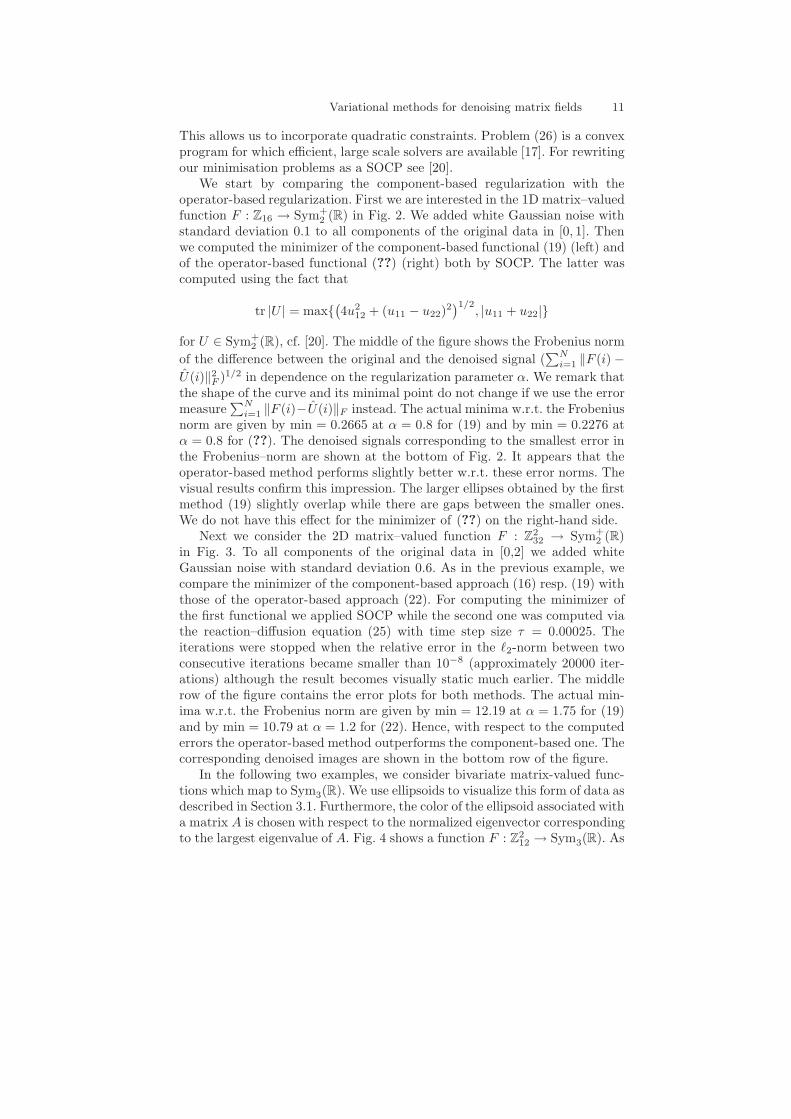
We start by comparing the component-based regularization with theoperator-based regularization. First we are interested in the 1D matrix–valuedfunction F : Z16 → Sym+

2 (R) in Fig. 2. We added white Gaussian noise withstandard deviation 0.1 to all components of the original data in [0, 1]. Thenwe computed the minimizer of the component-based functional (19) (left) andof the operator-based functional (??) (right) both by SOCP. The latter wascomputed using the fact that

tr |U | = max(

4u212 + (u11 − u22)

2)1/2

, |u11 + u22|

for U ∈ Sym+2 (R), cf. [20]. The middle of the figure shows the Frobenius norm

of the difference between the original and the denoised signal (∑N

i=1 ‖F (i) −U(i)‖2

F )1/2 in dependence on the regularization parameter α. We remark thatthe shape of the curve and its minimal point do not change if we use the errormeasure

∑Ni=1 ‖F (i)−U(i)‖F instead. The actual minima w.r.t. the Frobenius

norm are given by min = 0.2665 at α = 0.8 for (19) and by min = 0.2276 atα = 0.8 for (??). The denoised signals corresponding to the smallest error inthe Frobenius–norm are shown at the bottom of Fig. 2. It appears that theoperator-based method performs slightly better w.r.t. these error norms. Thevisual results confirm this impression. The larger ellipses obtained by the firstmethod (19) slightly overlap while there are gaps between the smaller ones.We do not have this effect for the minimizer of (??) on the right-hand side.

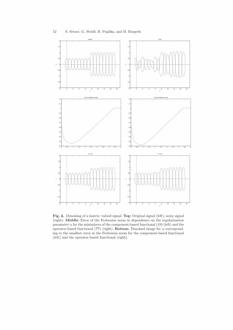
Next we consider the 2D matrix–valued function F : Z232 → Sym+

2 (R)in Fig. 3. To all components of the original data in [0,2] we added whiteGaussian noise with standard deviation 0.6. As in the previous example, wecompare the minimizer of the component-based approach (16) resp. (19) withthose of the operator-based approach (22). For computing the minimizer ofthe first functional we applied SOCP while the second one was computed viathe reaction–diffusion equation (25) with time step size τ = 0.00025. Theiterations were stopped when the relative error in the ℓ2-norm between twoconsecutive iterations became smaller than 10−8 (approximately 20000 iter-ations) although the result becomes visually static much earlier. The middlerow of the figure contains the error plots for both methods. The actual min-ima w.r.t. the Frobenius norm are given by min = 12.19 at α = 1.75 for (19)and by min = 10.79 at α = 1.2 for (22). Hence, with respect to the computederrors the operator-based method outperforms the component-based one. Thecorresponding denoised images are shown in the bottom row of the figure.

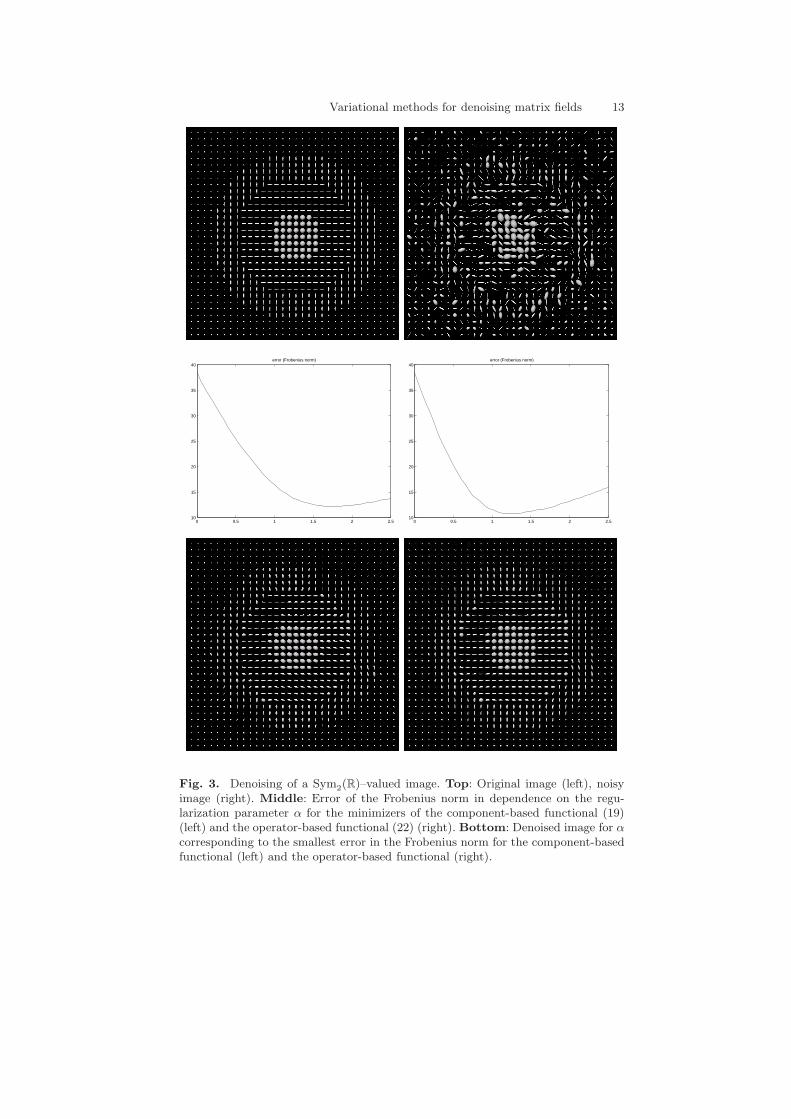
In the following two examples, we consider bivariate matrix-valued func-tions which map to Sym3(R). We use ellipsoids to visualize this form of data asdescribed in Section 3.1. Furthermore, the color of the ellipsoid associated witha matrix A is chosen with respect to the normalized eigenvector correspondingto the largest eigenvalue of A. Fig. 4 shows a function F : Z

212 → Sym3(R). As


−2 0 2 4 6 8 10 12 14 16−2

−1.5

−1

−0.5

0

0.5

1

1.5

2

x

y

original

−2 0 2 4 6 8 10 12 14 16−2

−1.5

−1

−0.5

0

0.5

1

1.5

2

x

y

noisy

0 0.5 1 1.5 2 2.5 3 3.5 4 4.5 50.2

0.3

0.4

0.5

0.6

0.7

0.8

0.9

1

1.1

1.2error (Frobenius norm)

0 0.5 1 1.5 2 2.5 3 3.5 4 4.5 50.2

0.3

0.4

0.5

0.6

0.7

0.8

0.9

1

1.1

1.2error (Frobenius norm)

x

y

α = 0.8

−2 0 2 4 6 8 10 12 14 16−2

−1.5

−1

−0.5

0

0.5

1

1.5

2

x

y

α = 0.8

−2 0 2 4 6 8 10 12 14 16−2

−1.5

−1

−0.5

0

0.5

1

1.5

2

Fig. 2. Denoising of a matrix–valued signal. Top: Original signal (left), noisy signal(right). Middle: Error of the Frobenius norm in dependence on the regularizationparameter α for the minimizers of the component-based functional (19) (left) and theoperator-based functional (??) (right). Bottom: Denoised image for α correspond-ing to the smallest error in the Frobenius norm for the component-based functional(left) and the operator-based functional (right).


0 0.5 1 1.5 2 2.510

15

20

25

30

35

40error (Frobenius norm)

0 0.5 1 1.5 2 2.510

15

20

25

30

35

40error (Frobenius norm)

Fig. 3. Denoising of a Sym2(R)–valued image. Top: Original image (left), noisy

image (right). Middle: Error of the Frobenius norm in dependence on the regu-larization parameter α for the minimizers of the component-based functional (19)(left) and the operator-based functional (22) (right). Bottom: Denoised image for α

corresponding to the smallest error in the Frobenius norm for the component-basedfunctional (left) and the operator-based functional (right).


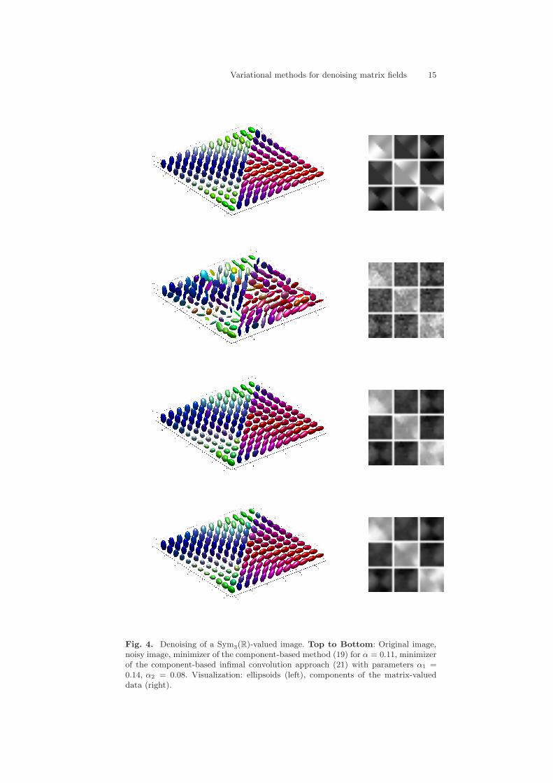
before, we added white Gaussian noise to all components. The matrix compo-nents of the original data lie in the interval [−0.5, 0.5] and the standard devi-ation of the Gaussian noise is 0.06. The denoising results are displayed in thelast two rows of Fig. 4. We computed the minimizers of the component-basedmethod (19) (top) by SOCP. The smallest error, measured in the Frobenius-norm, is 1.102 and was obtained for the regularization parameter α = 0.11.In addition, we considered the minimizer of the infimal convolution approach(21) (bottom). Again we applied SOCP and found the optimal regularizationparameters to be α1 = 0.14 and α2 = 0.08 for this method. The correspondingFrobenius-norm error is 0.918. We see that the infimal convolution approachis also suited for matrix-valued data.

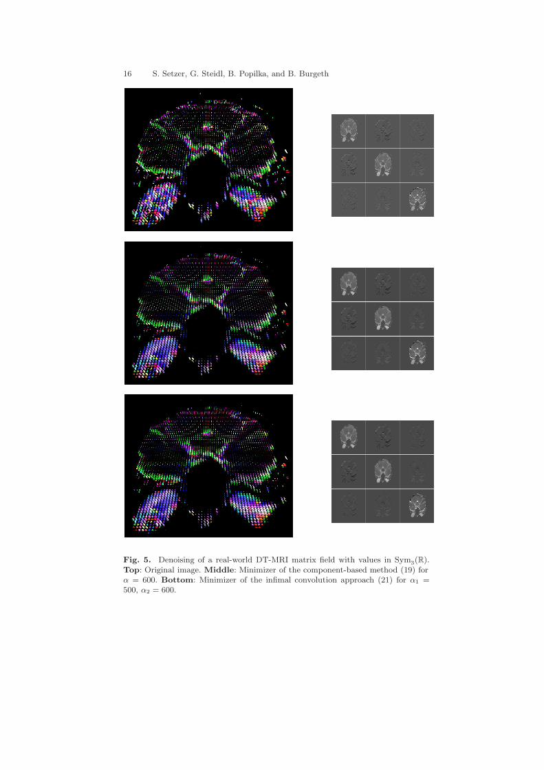
In our final experiment, we applied the two component-based methods (19)and (21) to a larger data set. Fig. 5 shows the orginal data and the minimizersof (19) and (21). The components of the original data lie in [−4000, 7000] andwe used the regularization parameters α = 600 for (19) and α1 = 500, α2 =600 for (21), respectively.

A Proofs

Proof of Proposition 1. Using that the minimal and maximal eigenvaluesλmin(A), λmax(A) of a symmetric matrix A fulfill

λmin(A) = min‖v‖=1

vTAv, λmax(A) = max‖v‖=1

vTAv,

it is easy to check that the set C of matrices having all eigenvalues in[λmin, λmax] is convex and closed. Let J be the functional in (19). Assumethat some matrices U(i, j) are not contained in C. Let PU(i, j) denote theorthogonal projection (w.r.t. the Frobenius norm) of U(i, j) onto C. Then weobtain by the projection theorem [11, p. 269] that

‖F (i, j)− PU(i, j)‖F ≤ ‖F (i, j) − U(i, j)‖F ,

‖PU(i, j) − PU(k, l)‖F ≤ ‖U(i, j) − U(k, l)‖F .

Consequently, J (PU) ≤ J (U) which contradicts our assumption since theminimizer is unique. This completes the proof.

Proof of Proposition 2. Since ‖F − U‖2F is strictly convex, it remains to

show that the functional

J(U) := tr(√

U2x + U2

y

)

is convex. Moreover, since J is positively homogeneous we only have to provethat J is subadditive, cf. [2, p. 34], i.e.,

J(U + U) ≤ J(U) + J(U).


Fig. 4. Denoising of a Sym3(R)-valued image. Top to Bottom: Original image,

noisy image, minimizer of the component-based method (19) for α = 0.11, minimizerof the component-based infimal convolution approach (21) with parameters α1 =0.14, α2 = 0.08. Visualization: ellipsoids (left), components of the matrix-valueddata (right).


Fig. 5. Denoising of a real-world DT-MRI matrix field with values in Sym3(R).

Top: Original image. Middle: Minimizer of the component-based method (19) forα = 600. Bottom: Minimizer of the infimal convolution approach (21) for α1 =500, α2 = 600.


This can be rewritten as

tr

(

√

(Ux + Ux)2 + (Uy + Uy)2)

≤ tr

(

√

U2x + U2

y

)

+ tr(√

U2x + U2

y

)

.

To prove this relation, we recall the definition of the trace norm, cf. [14, p.197], which is defined as the sum of the singular values of a matrix A ∈ R

s,t:

‖A‖tr = tr(√

A∗A).

Then we have for the symmetric matrices Ux, Uy, Ux, Uy that

‖(

Ux + Ux

Uy + Uy

)

‖tr = tr

(

√

(Ux + Ux)2 + (Uy + Uy)2)

Since ‖ · ‖tr is a norm it follows that

‖(

Ux + Ux

Uy + Uy

)

‖tr ≤ ‖(

Ux

Uy

)

‖tr + ‖(

Ux

Uy

)

‖tr

= tr(√

U2x + U2

y ) + tr(√

U2x + U2

y )

and we are done.

Proof of Proposition 3. Let ϕ(Ux, Uy) := tr(

Φ(U2x + U2

y ))

. The Euler-Lagrange equations of (22) are given, for i, j = 1, ..., n and i ≥ j, by

0 =∂

∂uij‖F − U‖2

F − α

(

∂

∂x

(

∂ϕ

∂uijx

)

+∂

∂y

(

∂ϕ

∂uijy

))

.

For a scalar-valued function f and an n × n matrix X , we set ∂f(X)∂X :=

(

∂f(X)∂xij

)n

i,j=1. Then, by symmetry of F and U , the Euler-Lagrange equations

can be rewritten in matrix-vector form as

Wn U − F

α=

1

2

(

∂

∂x

(

∂ϕ

∂Ux

)

+∂

∂y

(

∂ϕ

∂Uy

))

, (27)

where Wn denotes the n × n matrix with diagonal entries 1 and other coeffi-cients 2, and AB stands for the Hadamard product (componentwise product)of A and B.We consider f(X) := tr Φ(X2). Then we obtain by [16, p. 178] and tr (ATB) =(vecA)TvecB that

vec∂f(X)

∂X= vec

(

tr (Φ′(X2)∂(X2)

∂xij)

)n

i,j=1

= vec

(

(vecΨ)Tvec∂(X2)

∂xij

)n

i,j=1


where Ψ := Φ′(X2). By [16, p. 182] and since Ψ is symmetric this can berewritten as

vec∂f(X)

∂X= vec Wn ((In ⊗ X) + (X ⊗ In)) vec Ψ.

Using that vec(ABC) = (CT ⊗ A)vecB we infer that

vec∂f(X)

∂X= vecWn vec(XΨ + ΨX).

This implies that∂f(X)

∂X= 2 Wn (Ψ • X). (28)

Applying (28) with f(Ux) := ϕ(Ux, Uy) and f(Uy) := ϕ(Ux, Uy), respectively,in (27) we obtain the assertion.

Acknowledgements. The authors like to thank J. Weickert and S. Didasfor fruitful discussions.

References

1. A. Barvinok. A Course in Convexity, Graduate Studies in Mathematics. AMS,Providence, RI, 2002.

2. J. M. Borwein and A. S. Lewis. Convex Analysis and Nonlinear Optimization.Springer, New York, 2000.

3. T. Brox, J. Weickert, B. Burgeth, and P. Mrazek. Nonlinear structure tensors.Image and Vision Computing, 24(1):41–55, 2006.

4. B. Burgeth, A. Bruhn, S. Didas, J. Weickert, and M. Welk. Morphology formatrix-data: Ordering versus PDE-based approach. Image and Vision Comput-

ing, 25(4):496–511, 2007.5. B. Burgeth, A. Bruhn, N. Papenberg, M. Welk, and J. Weickert. Mathemat-

ical morphology for matrix fields induced by the Loewner ordering in higherdimensions. Signal Processing, 87(2):277–290, 2007.

6. B. Burgeth, S. Didas, L. Florack, and J. Weickert. Singular PDEs for theprocessing of matrix-valued data. Lecture Notes in Computer Science. Springer,Berlin, 2007. To appear.

7. B. Burgeth, S. Didas, and J. Weickert. A generic approach to diffusion filteringof matrix-fields. Computing. Submitted.

8. A. Chambolle. An algorithm for total variation minimization and applications.Journal of Mathematical Imaging and Vision, (20):89–97, 2004.

9. A. Chambolle and P.-L. Lions. Image recovery via total variation minimizationand related problems. Numerische Mathematik, 76:167–188, 1997.

10. C. Chefd’Hotel, D. Tschumperle, R. Deriche, and O. Faugeras. Constrainedflows of matrix-valued functions: Application to diffusion tensor regularization.In A. Heyden, G. Sparr, M. Nielsen, and P. Johansen, editors, Computer Vision

– ECCV 2002, volume 2350 of Lecture Notes in Computer Science, pages 251–265. Springer, Berlin, 2002.


11. P. G. Ciarlet. Introduction to Numerical Linear Algebra and Optimisation. Cam-bridge University Press, Cambridge, 1989.

12. S. Didas, G. Steidl, and S. Setzer. Combined ℓ2 data and gradient fitting inconjunction with ℓ1 regularization. Adv. Comput. Math., 2007, accepted.

13. D. Goldfarb and W. Yin. Second-order cone programming methods for totalvariation-based image restoration. SIAM J. Scientific Computing, 2(27):622–645, 2005.

14. R. A. Horn and C. R. Johnson. Topics in Matrix Analysis. Cambridge UniversityPress, Cambridge, U.K., 1991.

15. S. B. M. S. Lobo, L. Vandenberghe and H. Lebret. Applications of second-ordercone programming. Linear Algebra and its Applications, 1998.

16. J. R. Magnus and H. Neudecker. Matrix Differential Calculus with Applications

in Statistics and Econometrics. J. Wiley and Sons, Chichester, 1988.17. H. Mittelmann. An independent bechmarking of SDP and SOCP solvers. Math-

ematical Programming Series B, 95(2):407–430, 2003.18. L. I. Rudin, S. Osher, and E. Fatemi. Nonlinear total variation based noise

removal algorithms. Physica A, 60:259–268, 1992.19. O. Scherzer and J. Weickert. Relations between regularization and diffusion

filtering. Journal of Mathematical Imaging and Vision, 12(1):43–63, Feb. 2000.20. G. Steidl, S. Setzer, B. Popilka, and B. Burgeth. Restoration of matrix fields

by second-order cone programming. Computing, 2007, submitted.21. D. Tschumperle and R. Deriche. Diffusion tensor regularization with constraints

preservation. In Proc. 2001 IEEE Computer Society Conference on Computer

Vision and Pattern Recognition, volume 1, pages 948–953, Kauai, HI, Dec. 2001.IEEE Computer Society Press.

22. D. Tschumperle and R. Deriche. Diffusion tensor regularization with contraintspreservation. In Proc. 2001 IEEE Computer Society Conference on Computer

Vision and Pattern Recognition, volume 1, pages 948–953, Kauai, HI, 2001.IEEE Computer Science Press.

23. J. Weickert. Anisotropic Diffusion in Image Processing. Teubner, Stuttgart,1998.

24. J. Weickert and T. Brox. Diffusion and regularization of vector- and matrix-valued images. In M. Z. Nashed and O. Scherzer, editors, Inverse Problems,

Image Analysis, and Medical Imaging, volume 313 of Contemporary Mathemat-

ics, pages 251–268. AMS, Providence, 2002.25. J. Weickert and H. Hagen, editors. Visualization and Processing of Tensor

Fields. Springer, Berlin, 2006.

Variational methods for denoising matrix ﬁelds · Variational methods for denoising matrix...

Documents

Transcript of Variational methods for denoising matrix ﬁelds · Variational methods for denoising matrix...