Variational Inference for Beta-Bernoulli DirichletProcess Mixture Models

Mengrui Ni, Erik B. Sudderth (Advisor), Mike Hughes (Advisor)Department of Computer Science, Brown University

mni@cs.brown.edu, sudderth@cs.brown.edu, mhughes@cs.brown.edu

Abstract

A commonly used paradigm in diverse application areas is to assume that an observed setof individual binary features is generated from a Bernoulli distribution with probabilitiesvarying according to a Beta distribution. In this paper, we present our nonparametricvariational inference algorithm for the Beta-Bernoulli observation model. Our primary focusis clustering discrete binary data using the Dirichlet process (DP) mixture model.

1 Introduction

In many biological and vision studies, the presences and absences of a certain set of engineered attributescreate binary outcomes which can be used to describe and distinguish individual objects. Observations ofsuch discrete binary feature data are usually assumed to be generated from mixtures of Bernoulli distributionswith probability parameters µ governed by Beta distributions. Such a model, also known as latent classanalysis [6], is practically important in its own right. Our discussion will focus on clustering discrete binarydata via the Dirichlet process (DP) mixture model.

2 Beta-Bernoulli Observation Model

The Beta-Bernoulli model is one of the simplest Bayesian models with Bernoulli likelihood p(X | µ) and itsconjugate Beta prior p(µ).

2.1 Bernoulli distribution

Consider a binary dataset with N observations and D attributes:

X =

x11 x12 · · · x1Dx21 x22 · · · x2D

......

. . ....

xN1 xN2 · · · xND

,

where X1, X2, . . . , XN ∼ i.i.d. Bernoulli(X | µ). Each Xi is a vector of 0’s and 1’s.For a single Bernoulli distribution, the probability density for each observation has the following form:

p(Xi | µ) =D∏d=1

µxid

d (1− µd)1−xid . (1)

1

Now, let’s consider a mixture of K Bernoulli distributions. Each component has weight πk, where∑Kk=1 πk =

1. Then, the density function for each observation can be expressed as follows:

p(Xi | µ, π) =K∑k=1

πk p(Xi | µk), (2)

where µ = [µ1, . . . , µK ], π = [π1, . . . , πK ], and p(Xi | µk) =∏Dd=1 µ

xid

kd (1− µkd)1−xid .

2.2 Beta distribution

The conjugate prior to the Bernoulli likelihood is the Beta distribution. A Beta distribution is parameterizedby two hyperparameters β0 and β1, which are positive real numbers. The distribution has support over theinterval [0, 1], and is defined as follows:

p(µ | β1, β0) =1

B(β1, β0) µ β1−1(1− µ) β0−1, µ ∈ [0, 1]. (3)

where B(β1, β0) =∫ 1

0 µβ1−1(1− µ) β0−1 dµ is the beta function, which also has the form,

B(β1, β0) =Γ(β1)Γ(β0)Γ(β1 + β0) , β0, β1 > 0. (4)

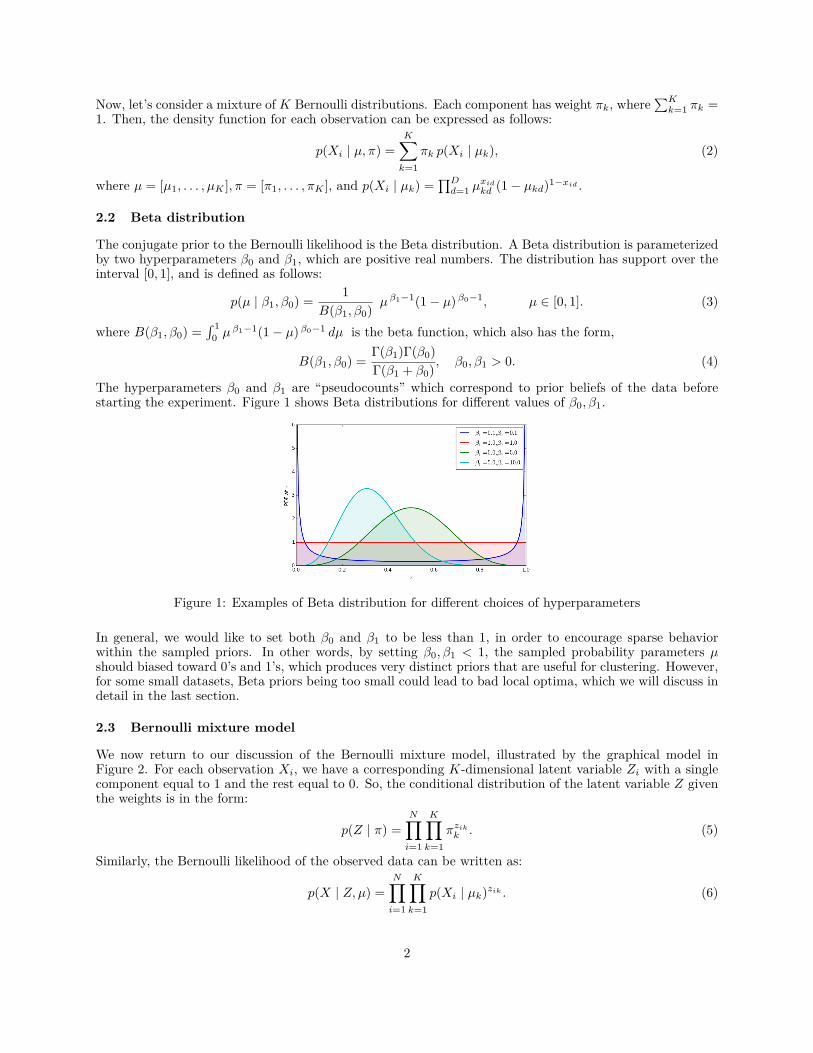
The hyperparameters β0 and β1 are “pseudocounts” which correspond to prior beliefs of the data beforestarting the experiment. Figure 1 shows Beta distributions for different values of β0, β1.

Figure 1: Examples of Beta distribution for different choices of hyperparameters

In general, we would like to set both β0 and β1 to be less than 1, in order to encourage sparse behaviorwithin the sampled priors. In other words, by setting β0, β1 < 1, the sampled probability parameters µshould biased toward 0’s and 1’s, which produces very distinct priors that are useful for clustering. However,for some small datasets, Beta priors being too small could lead to bad local optima, which we will discuss indetail in the last section.

2.3 Bernoulli mixture model

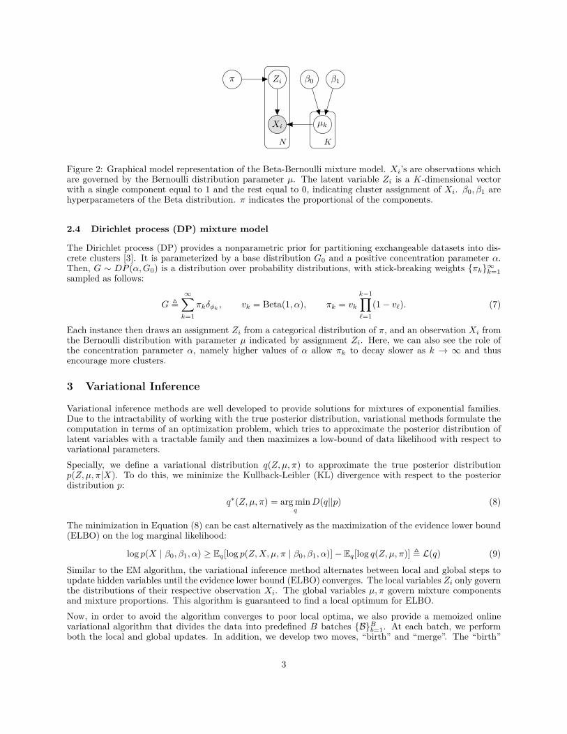
We now return to our discussion of the Bernoulli mixture model, illustrated by the graphical model inFigure 2. For each observation Xi, we have a corresponding K-dimensional latent variable Zi with a singlecomponent equal to 1 and the rest equal to 0. So, the conditional distribution of the latent variable Z giventhe weights is in the form:

p(Z | π) =N∏i=1

K∏k=1

πzik

k . (5)

Similarly, the Bernoulli likelihood of the observed data can be written as:

p(X | Z, µ) =N∏i=1

K∏k=1

p(Xi | µk)zik . (6)

2

Xi

Ziπ

µk

β0 β1

N K

Figure 2: Graphical model representation of the Beta-Bernoulli mixture model. Xi’s are observations whichare governed by the Bernoulli distribution parameter µ. The latent variable Zi is a K-dimensional vectorwith a single component equal to 1 and the rest equal to 0, indicating cluster assignment of Xi. β0, β1 arehyperparameters of the Beta distribution. π indicates the proportional of the components.

2.4 Dirichlet process (DP) mixture model

The Dirichlet process (DP) provides a nonparametric prior for partitioning exchangeable datasets into dis-crete clusters [3]. It is parameterized by a base distribution G0 and a positive concentration parameter α.Then, G ∼ DP (α,G0) is a distribution over probability distributions, with stick-breaking weights {πk}∞k=1sampled as follows:

G ,∞∑k=1

πkδφk, vk = Beta(1, α), πk = vk

k−1∏`=1

(1− v`). (7)

Each instance then draws an assignment Zi from a categorical distribution of π, and an observation Xi fromthe Bernoulli distribution with parameter µ indicated by assignment Zi. Here, we can also see the role ofthe concentration parameter α, namely higher values of α allow πk to decay slower as k → ∞ and thusencourage more clusters.

3 Variational Inference

Variational inference methods are well developed to provide solutions for mixtures of exponential families.Due to the intractability of working with the true posterior distribution, variational methods formulate thecomputation in terms of an optimization problem, which tries to approximate the posterior distribution oflatent variables with a tractable family and then maximizes a low-bound of data likelihood with respect tovariational parameters.Specially, we define a variational distribution q(Z, µ, π) to approximate the true posterior distributionp(Z, µ, π|X). To do this, we minimize the Kullback-Leibler (KL) divergence with respect to the posteriordistribution p:

q∗(Z, µ, π) = arg minq

D(q||p) (8)

The minimization in Equation (8) can be cast alternatively as the maximization of the evidence lower bound(ELBO) on the log marginal likelihood:

log p(X | β0, β1, α) ≥ Eq[log p(Z,X, µ, π | β0, β1, α)]− Eq[log q(Z, µ, π)] , L(q) (9)

Similar to the EM algorithm, the variational inference method alternates between local and global steps toupdate hidden variables until the evidence lower bound (ELBO) converges. The local variables Zi only governthe distributions of their respective observation Xi. The global variables µ, π govern mixture componentsand mixture proportions. This algorithm is guaranteed to find a local optimum for ELBO.Now, in order to avoid the algorithm converges to poor local optima, we also provide a memoized onlinevariational algorithm that divides the data into predefined B batches {B}Bb=1. At each batch, we performboth the local and global updates. In addition, we develop two moves, “birth” and “merge”. The “birth”

3

move can add useful new components to the model and escape poor local optima. The “merge” move, onthe other hand, combines two components into a single merged one. In one pass of the data, the memoizedalgorithm performs a “birth” move for all batches, and several “merge” moves after the final batch.

4 Experiments

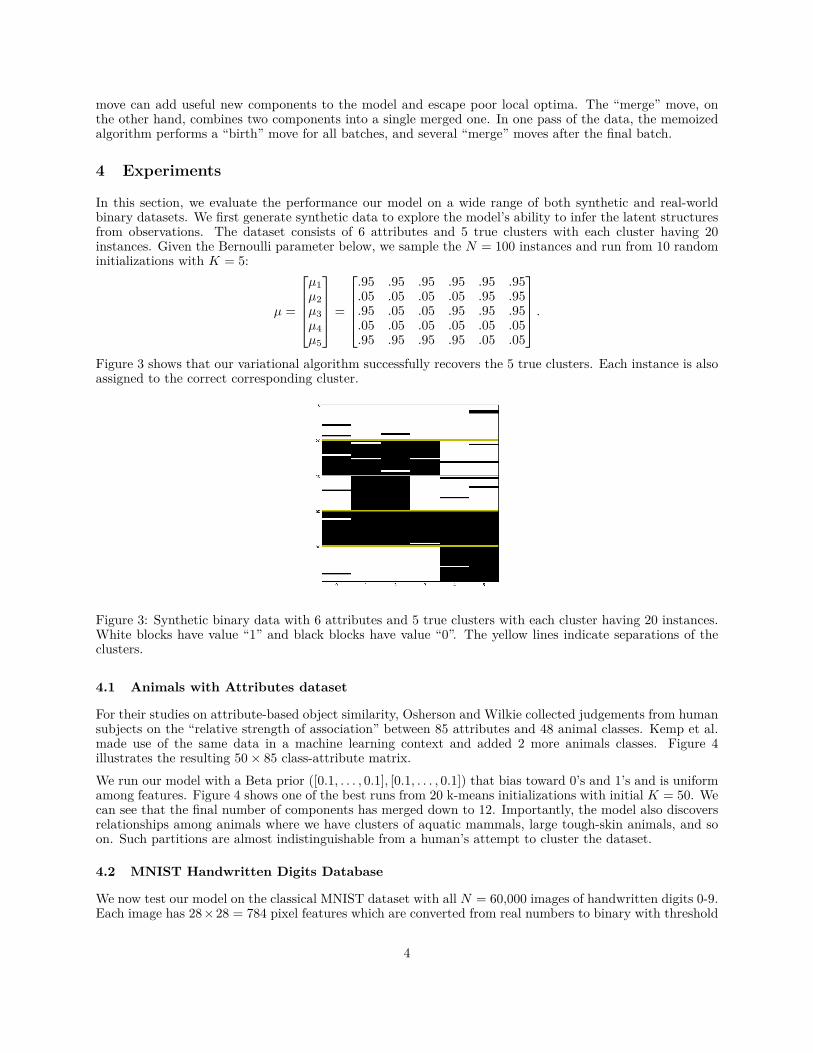
In this section, we evaluate the performance our model on a wide range of both synthetic and real-worldbinary datasets. We first generate synthetic data to explore the model’s ability to infer the latent structuresfrom observations. The dataset consists of 6 attributes and 5 true clusters with each cluster having 20instances. Given the Bernoulli parameter below, we sample the N = 100 instances and run from 10 randominitializations with K = 5:

µ =

µ1µ2µ3µ4µ5

=

.95 .95 .95 .95 .95 .95.05 .05 .05 .05 .95 .95.95 .05 .05 .95 .95 .95.05 .05 .05 .05 .05 .05.95 .95 .95 .95 .05 .05

.Figure 3 shows that our variational algorithm successfully recovers the 5 true clusters. Each instance is alsoassigned to the correct corresponding cluster.

Figure 3: Synthetic binary data with 6 attributes and 5 true clusters with each cluster having 20 instances.White blocks have value “1” and black blocks have value “0”. The yellow lines indicate separations of theclusters.

4.1 Animals with Attributes dataset

For their studies on attribute-based object similarity, Osherson and Wilkie collected judgements from humansubjects on the “relative strength of association” between 85 attributes and 48 animal classes. Kemp et al.made use of the same data in a machine learning context and added 2 more animals classes. Figure 4illustrates the resulting 50× 85 class-attribute matrix.We run our model with a Beta prior ([0.1, . . . , 0.1], [0.1, . . . , 0.1]) that bias toward 0’s and 1’s and is uniformamong features. Figure 4 shows one of the best runs from 20 k-means initializations with initial K = 50. Wecan see that the final number of components has merged down to 12. Importantly, the model also discoversrelationships among animals where we have clusters of aquatic mammals, large tough-skin animals, and soon. Such partitions are almost indistinguishable from a human’s attempt to cluster the dataset.

4.2 MNIST Handwritten Digits Database

We now test our model on the classical MNIST dataset with all N = 60,000 images of handwritten digits 0-9.Each image has 28×28 = 784 pixel features which are converted from real numbers to binary with threshold

4

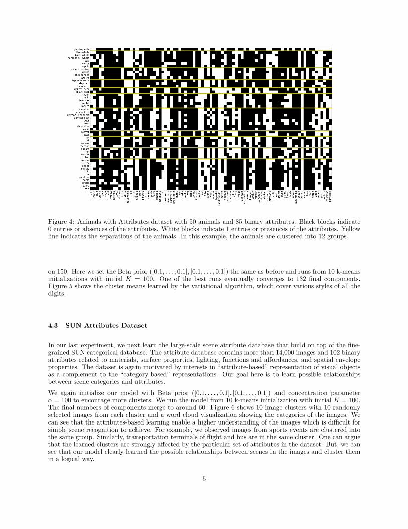
Figure 4: Animals with Attributes dataset with 50 animals and 85 binary attributes. Black blocks indicate0 entries or absences of the attributes. White blocks indicate 1 entries or presences of the attributes. Yellowline indicates the separations of the animals. In this example, the animals are clustered into 12 groups.

on 150. Here we set the Beta prior ([0.1, . . . , 0.1], [0.1, . . . , 0.1]) the same as before and runs from 10 k-meansinitializations with initial K = 100. One of the best runs eventually converges to 132 final components.Figure 5 shows the cluster means learned by the variational algorithm, which cover various styles of all thedigits.

4.3 SUN Attributes Dataset

In our last experiment, we next learn the large-scale scene attribute database that build on top of the fine-grained SUN categorical database. The attribute database contains more than 14,000 images and 102 binaryattributes related to materials, surface properties, lighting, functions and affordances, and spatial envelopeproperties. The dataset is again motivated by interests in “attribute-based” representation of visual objectsas a complement to the “category-based” representations. Our goal here is to learn possible relationshipsbetween scene categories and attributes.We again initialize our model with Beta prior ([0.1, . . . , 0.1], [0.1, . . . , 0.1]) and concentration parameterα = 100 to encourage more clusters. We run the model from 10 k-means initialization with initial K = 100.The final numbers of components merge to around 60. Figure 6 shows 10 image clusters with 10 randomlyselected images from each cluster and a word cloud visualization showing the categories of the images. Wecan see that the attributes-based learning enable a higher understanding of the images which is difficult forsimple scene recognition to achieve. For example, we observed images from sports events are clustered intothe same group. Similarly, transportation terminals of flight and bus are in the same cluster. One can arguethat the learned clusters are strongly affected by the particular set of attributes in the dataset. But, we cansee that our model clearly learned the possible relationships between scenes in the images and cluster themin a logical way.

5

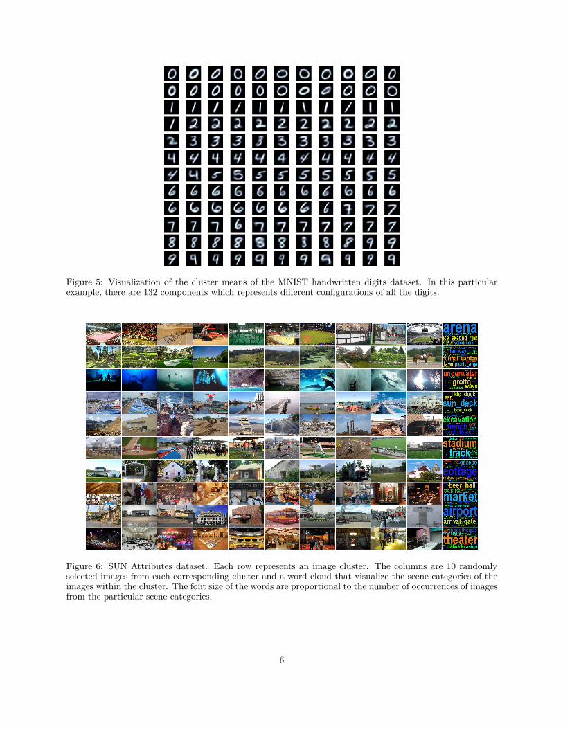
Figure 5: Visualization of the cluster means of the MNIST handwritten digits dataset. In this particularexample, there are 132 components which represents different configurations of all the digits.

Figure 6: SUN Attributes dataset. Each row represents an image cluster. The columns are 10 randomlyselected images from each corresponding cluster and a word cloud that visualize the scene categories of theimages within the cluster. The font size of the words are proportional to the number of occurrences of imagesfrom the particular scene categories.

6

5 Discussions and Conclusions

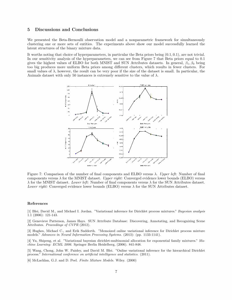
We presented the Beta-Bernoulli observation model and a nonparametric framework for simultaneouslyclustering one or more sets of entities. The experiments above show our model successfully learned thelatent structures of the binary mixture data.It worths noting that choice of hyperparameters, in particular the Beta priors being (0.1, 0.1), are not trivial.In our sensitivity analysis of the hyperparameters, we can see from Figure 7 that Beta priors equal to 0.1gives the highest values of ELBO for both MNIST and SUN Attributes datasets. In general, β1, β0 beingtoo big produces more uniform Beta priors among different clusters, which results in fewer clusters. Forsmall values of λ, however, the result can be very poor if the size of the dataset is small. In particular, theAnimals dataset with only 50 instances is extremely sensitive to the value of λ.

Figure 7: Comparison of the number of final components and ELBO versus λ. Upper left: Number of finalcomponents versus λ for the MNIST dataset. Upper right: Converged evidence lower bounds (ELBO) versusλ for the MNIST dataset. Lower left: Number of final components versus λ for the SUN Attributes dataset.Lower right: Converged evidence lower bounds (ELBO) versus λ for the SUN Attributes dataset.

References

[1] Blei, David M., and Michael I. Jordan. ”Variational inference for Dirichlet process mixtures.” Bayesian analysis1.1 (2006): 121-143.

[2] Genevieve Patterson, James Hays. SUN Attribute Database: Discovering, Annotating, and Recognizing SceneAttributes. Proceedings of CVPR (2012).

[3] Hughes, Michael C., and Erik Sudderth. ”Memoized online variational inference for Dirichlet process mixturemodels.” Advances in Neural Information Processing Systems. (2013): (pp. 1133-1141).

[4] Yu, Shipeng, et al. ”Variational bayesian dirichlet-multinomial allocation for exponential family mixtures.” Ma-chine Learning: ECML 2006. Springer Berlin Heidelberg, (2006). 841-848.

[5] Wang, Chong, John W. Paisley, and David M. Blei. ”Online variational inference for the hierarchical Dirichletprocess.” International conference on artificial intelligence and statistics. (2011).

[6] McLachlan, G.J. and D. Peel. Finite Mixture Models. Wiley. (2000)

7

[7] Hughes, Michael C., Dae Il Kim, and Erik B. Sudderth. ”Reliable and Scalable Variational Inference for theHierarchical Dirichlet Process.” Proceedings of the Eighteenth International Conference on Artificial Intelligence andStatistics. (2015).

8