Variational Inference for Bayesian Neural NetworksVariational Inference for Bayesian Neural Networks...
82
Variational Inference for Bayesian Neural Networks Jesse Bettencourt, Harris Chan, Ricky Chen, Elliot Creager, Wei Cui, Mo- hammad Firouzi, Arvid Frydenlund, Amanjit Singh Kainth, Xuechen Li, Jeff Wintersinger, Bowen Xu October 6, 2017 University of Toronto 1
Transcript of Variational Inference for Bayesian Neural NetworksVariational Inference for Bayesian Neural Networks...
Variational Inference for Bayesian Neural
Networks
Jesse Bettencourt, Harris Chan, Ricky Chen, Elliot Creager, Wei Cui, Mo-
hammad Firouzi, Arvid Frydenlund, Amanjit Singh Kainth, Xuechen Li,
Jeff Wintersinger, Bowen Xu
October 6, 2017
University of Toronto
1
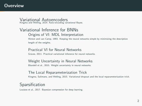
Overview
Variational AutoencodersKingma and Welling, 2014. Auto-encoding variational Bayes.
Variational Inference for BNNsOrigins of VI: MDL InterpretationHinton and van Camp, 1993. Keeping the neural networks simple by minimizing the description
length of the weights.
Practical VI for Neural NetworksGraves, 2011. Practical variational inference for neural networks.
Weight Uncertainty in Neural NetworksBlundell et al., 2015. Weight uncertainty in neural networks.
The Local Reparameterization TrickKingma, Salimans, and Welling, 2015. Variational dropout and the local reparameterization trick.
SparsificationLouizos et al., 2017. Bayesian compression for deep learning.
2
Variational Autoencoders (VAE)
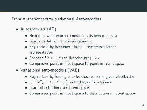
From Autoencoders to Variational Autoencoders
• Autoencoders (AE)
• Neural network which reconstructs its own inputs, x
• Learns useful latent representation, z
• Regularized by bottleneck layer – compresses latent
representation
• Encoder f (x)→ z and decoder g(z)→ x
• Compresses point in input space to point in latent space
• Variational autoencoders (VAE)
• Regularized by forcing z to be close to some given distribution
• z ∼ N (µ = 0, σ2 = 1), with diagonal covariance
• Learn distribution over latent space
• Compresses point in input space to distribution in latent space
3
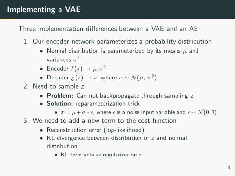
Implementing a VAE
Three implementation differences between a VAE and an AE
1. Our encoder network parameterizes a probability distribution
• Normal distribution is parameterized by its means µ and
variances σ2
• Encoder f (x)→ µ, σ2
• Decoder g(z)→ x , where z ∼ N (µ, σ2)
2. Need to sample z
• Problem: Can not backpropagate through sampling z
• Solution: reparameterization trick
• z = µ+σ ∗ ε, where ε is a noise input variable and ε ∼ N (0, 1)
3. We need to add a new term to the cost function
• Reconstruction error (log-likelihood)
• KL divergence between distribution of z and normal
distribution
• KL term acts as regularizer on z
4
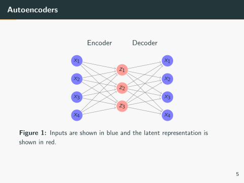
Autoencoders
x1
x2
x3
x4
z1
z2
z3
x1
x2
x3
x4
Encoder Decoder
Figure 1: Inputs are shown in blue and the latent representation is
shown in red.
5
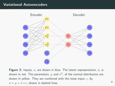
Variational Autoencoders
x1
x2
x3
x4
µ1
µ2
σ21
σ22
ε1
ε2
z1
z2
x1
x2
x3
x4
Encoder Decoder
Figure 2: Inputs, x , are shown in blue. The latent representation, z , is
shown in red. The parameters, µ and σ2, of the normal distribution are
shown in yellow. They are combined with the noise input, ε, by
z = µ+ σ ∗ ε, shown in dashed lines. 6
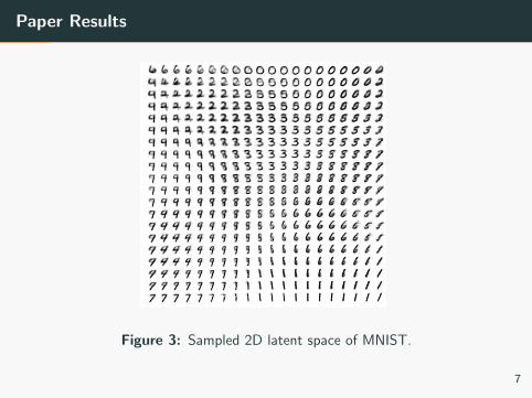
Paper Results
(a) Learned Frey Face manifold (b) Learned MNIST manifold
Figure 4: Visualisations of learned data manifold for generative models with two-dimensional latentspace, learned with AEVB. Since the prior of the latent space is Gaussian, linearly spaced coor-dinates on the unit square were transformed through the inverse CDF of the Gaussian to producevalues of the latent variables z. For each of these values z, we plotted the corresponding generativepθ(x|z) with the learned parameters θ.
(a) 2-D latent space (b) 5-D latent space (c) 10-D latent space (d) 20-D latent space
Figure 5: Random samples from learned generative models of MNIST for different dimensionalitiesof latent space.
B Solution of −DKL(qφ(z)||pθ(z)), Gaussian case
The variational lower bound (the objective to be maximized) contains a KL term that can often beintegrated analytically. Here we give the solution when both the prior pθ(z) = N (0, I) and theposterior approximation qφ(z|x(i)) are Gaussian. Let J be the dimensionality of z. Let µ and σdenote the variational mean and s.d. evaluated at datapoint i, and let µj and σj simply denote thej-th element of these vectors. Then:∫
qθ(z) log p(z) dz =
∫N (z;µ,σ2) logN (z;0, I) dz
= −J2log(2π)− 1
2
J∑j=1
(µ2j + σ2
j )
10
Figure 3: Sampled 2D latent space of MNIST.
7
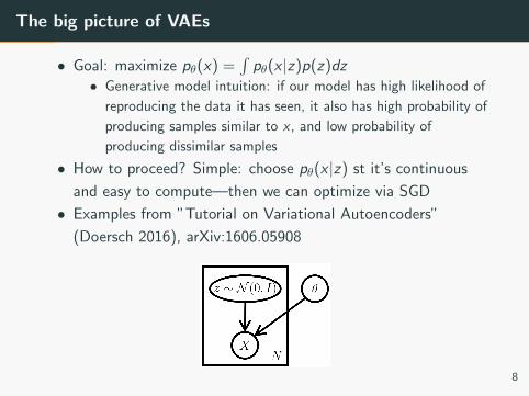
The big picture of VAEs
• Goal: maximize pθ(x) =∫
pθ(x |z)p(z)dz• Generative model intuition: if our model has high likelihood of
reproducing the data it has seen, it also has high probability of
producing samples similar to x , and low probability of
producing dissimilar samples
• How to proceed? Simple: choose pθ(x |z) st it’s continuous
and easy to compute—then we can optimize via SGD
• Examples from ”Tutorial on Variational Autoencoders”
(Doersch 2016), arXiv:1606.05908
8
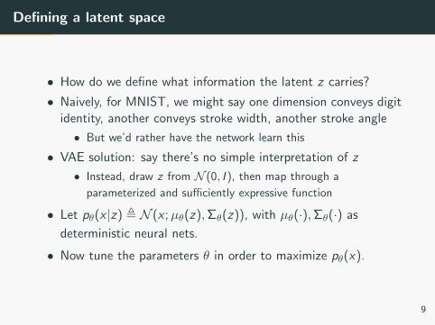
Defining a latent space
• How do we define what information the latent z carries?
• Naively, for MNIST, we might say one dimension conveys digitidentity, another conveys stroke width, another stroke angle
• But we’d rather have the network learn this
• VAE solution: say there’s no simple interpretation of z
• Instead, draw z from N (0, I ), then map through a
parameterized and sufficiently expressive function
• Let pθ(x |z) , N (x ;µθ(z),Σθ(z)), with µθ(·),Σθ(·) as
deterministic neural nets.
• Now tune the parameters θ in order to maximize pθ(x).
9
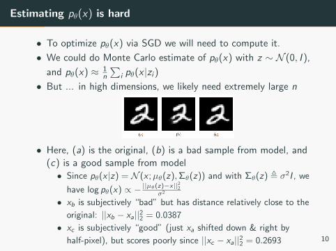
Estimating pθ(x) is hard
• To optimize pθ(x) via SGD we will need to compute it.
• We could do Monte Carlo estimate of pθ(x) with z ∼ N (0, I ),
and pθ(x) ≈ 1n
∑i pθ(x |zi )
• But ... in high dimensions, we likely need extremely large n
• Here, (a) is the original, (b) is a bad sample from model, and(c) is a good sample from model• Since pθ(x |z) = N (x ;µθ(z),Σθ(z)) and with Σθ(z) , σ2I , we
have log pθ(x) ∝ − ||µθ(z)−x||22σ2
• xb is subjectively “bad” but has distance relatively close to the
original: ||xb − xa||22 = 0.0387
• xc is subjectively “good” (just xa shifted down & right by
half-pixel), but scores poorly since ||xc − xa||22 = 0.2693 10
Sampling z values efficiently estimate pθ(x)
• Conclusion: to reject bad samples like xb, we must set σ2 tobe extremely small
• But this means that to get samples similar to xa, we’ll need to
sample a huge number of z values
• One solution: define better distance metric—but these are
difficult to engineer
• Better solution: sample only z that have non-negligible pθ(z |x)
• For most z sampled from p(z), we have pθ(x |z) ≈ 0, so
contribute almost nothing to pθ(x) estimate
• Idea: define function qφ(z |x) that helps us sample z with
non-negligible contribution to pθ(x)
11
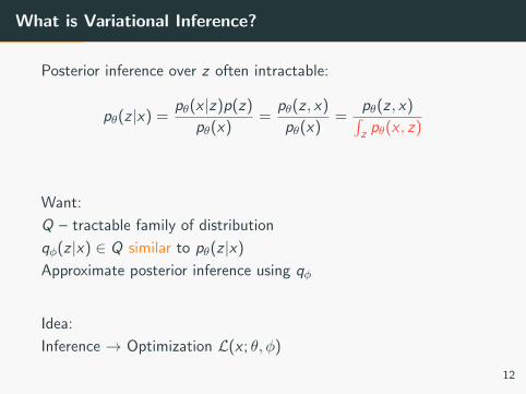
What is Variational Inference?
Posterior inference over z often intractable:
pθ(z |x) =pθ(x |z)p(z)
pθ(x)=
pθ(z , x)
pθ(x)=
pθ(z , x)∫z pθ(x , z)
Want:
Q – tractable family of distribution
qφ(z |x) ∈ Q similar to pθ(z |x)
Approximate posterior inference using qφ
Idea:
Inference → Optimization L(x ; θ, φ)
12
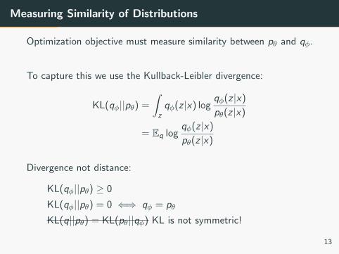
Measuring Similarity of Distributions
Optimization objective must measure similarity between pθ and qφ.
To capture this we use the Kullback-Leibler divergence:
KL(qφ||pθ) =
∫z
qφ(z |x) logqφ(z |x)
pθ(z |x)
= Eq logqφ(z |x)
pθ(z |x)
Divergence not distance:
KL(qφ||pθ) ≥ 0
KL(qφ||pθ) = 0 ⇐⇒ qφ = pθ
KL(q||pθ) = KL(pθ||qφ) KL is not symmetric!
13
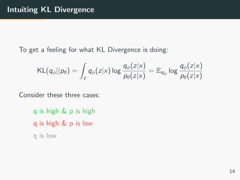
Intuiting KL Divergence
To get a feeling for what KL Divergence is doing:
KL(qφ||pθ) =
∫z
qφ(z |x) logqφ(z |x)
pθ(z |x)= Eqφ log
qφ(z |x)
pθ(z |x)
Consider these three cases:
q is high & p is high
q is high & p is low
q is low
14
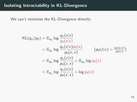
Isolating Intractability in KL-Divergence
We can’t minimize the KL-Divergence directly:
KL(qφ||pθ) = Eqφ logqφ(z |x)
pθ(z |x)
= Eqφ logqφ(z |x)pθ(x)
pθ(z , x)(pθ(z |x) = pθ(z,x)
pθ(x))
= Eqφ logqφ(z |x)
pθ(z , x)+ Eqφ log pθ(x)
= Eqφ logqφ(z |x)
pθ(z , x)+ log pθ(x)
15
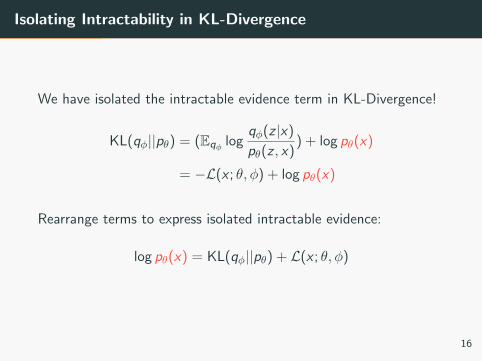
Isolating Intractability in KL-Divergence
We have isolated the intractable evidence term in KL-Divergence!
KL(qφ||pθ) = (Eqφ logqφ(z |x)
pθ(z , x)) + log pθ(x)
= −L(x ; θ, φ) + log pθ(x)
Rearrange terms to express isolated intractable evidence:
log pθ(x) = KL(qφ||pθ) + L(x ; θ, φ)
16
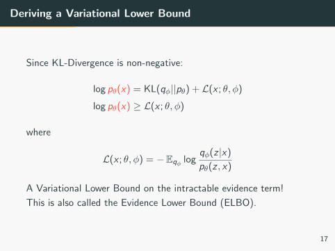
Deriving a Variational Lower Bound
Since KL-Divergence is non-negative:
log pθ(x) = KL(qφ||pθ) + L(x ; θ, φ)
log pθ(x) ≥ L(x ; θ, φ)
where
L(x ; θ, φ) = −Eqφ logqφ(z |x)
pθ(z , x)
A Variational Lower Bound on the intractable evidence term!
This is also called the Evidence Lower Bound (ELBO).
17
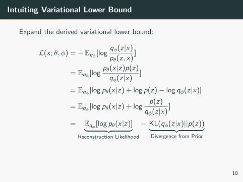
Intuiting Variational Lower Bound
Expand the derived variational lower bound:
L(x ; θ, φ) = −Eqφ [logqφ(z |x)
pθ(z , x)]
= Eqφ [logpθ(x |z)p(z)
qφ(z |x)]
= Eqφ [log pθ(x |z) + log p(z)− log qφ(z |x)]
= Eqφ [log pθ(x |z) + logp(z)
qφ(z |x)]
= Eqφ [log pθ(x |z)]︸ ︷︷ ︸Reconstruction Likelihood
− KL(qφ(z |x)||p(z))︸ ︷︷ ︸Divergence from Prior
18
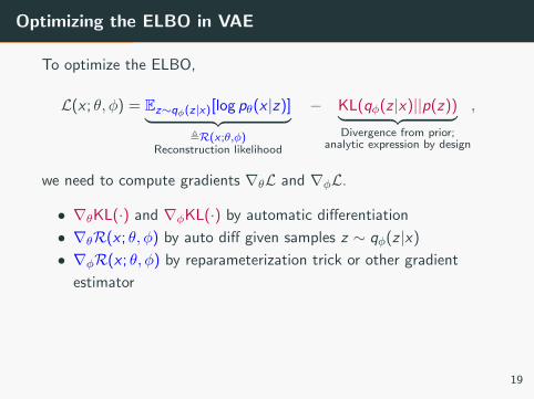
Optimizing the ELBO in VAE
To optimize the ELBO,
L(x ; θ, φ) = Ez∼qφ(z|x)[log pθ(x |z)]︸ ︷︷ ︸,R(x ;θ,φ)
Reconstruction likelihood
− KL(qφ(z |x)||p(z))︸ ︷︷ ︸Divergence from prior;
analytic expression by design
,
we need to compute gradients ∇θL and ∇φL.
• ∇θKL(·) and ∇φKL(·) by automatic differentiation
• ∇θR(x ; θ, φ) by auto diff given samples z ∼ qφ(z |x)
• ∇φR(x ; θ, φ) by reparameterization trick or other gradient
estimator
19
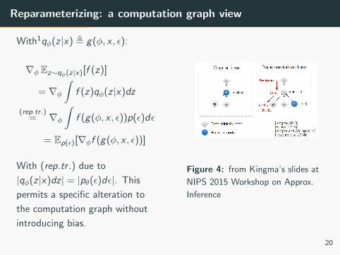
Reparameterizing: a computation graph view
With1qφ(z |x) , g(φ, x , ε):
∇φ Ez∼qφ(z|x)[f (z)]
= ∇φ∫
f (z)qφ(z |x)dz
(rep.tr .)= ∇φ
∫f (g(φ, x , ε))p(ε)dε
= Ep(ε)[∇φf (g(φ, x , ε))]
With (rep.tr .) due to
|qφ(z |x)dz | = |pθ(ε)dε|. This
permits a specific alteration to
the computation graph without
introducing bias.
Figure 4: from Kingma’s slides at
NIPS 2015 Workshop on Approx.
Inference
20
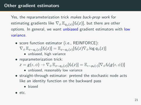
Other gradient estimators
Yes, the reparameterization trick makes back-prop work for
estimating gradients like ∇φ Eqφ(z)[fθ(z)], but there are other
options. In general, we want unbiased gradient estimators with low
variance.
• score function estimator (i.e., REINFORCE):∇φ Ez∼qφ(z)[fθ(z)] = Ez∼qφ(z)[fθ(z)∇φ log qφ(z)]
• unbiased, high variance
• reparameterization trick:z = g(ε, φ)→ ∇φ Ez∼qφ(z)[fθ(z)] = Eε∼pθ(ε)[∇φfθ(g(ε, φ))]
• unbiased, reasonably low variance
• straight-through estimator: pretend the stochastic node actslike an identity function on the backward pass
• biased
• etc.
21
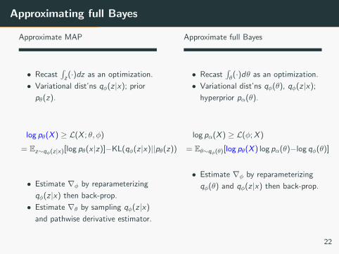
Approximating full Bayes
Approximate MAP
• Recast∫z(·)dz as an optimization.
• Variational dist’ns qφ(z |x); prior
pθ(z).
log pθ(X ) ≥ L(X ; θ, φ)
= Ez∼qφ(z|x)[log pθ(x |z)]−KL(qφ(z |x)||pθ(z))
• Estimate ∇φ by reparameterizing
qφ(z |x) then back-prop.
• Estimate ∇θ by sampling qφ(z |x)
and pathwise derivative estimator.
Approximate full Bayes
• Recast∫θ(·)dθ as an optimization.
• Variational dist’ns qφ(θ), qφ(z |x);
hyperprior pα(θ).
log pα(X ) ≥ L(φ; X )
= Eθ∼qφ(θ)[log pθ(X ) log pα(θ)−log qφ(θ)]
• Estimate ∇φ by reparameterizing
qφ(θ) and qφ(z |x) then back-prop.
22
Variational Inference for BNNs
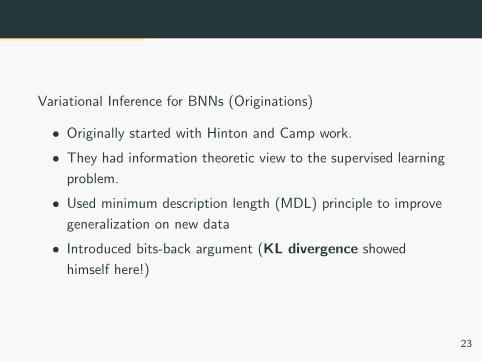
Variational Inference for BNNs (Originations)
• Originally started with Hinton and Camp work.
• They had information theoretic view to the supervised learning
problem.
• Used minimum description length (MDL) principle to improve
generalization on new data
• Introduced bits-back argument (KL divergence showed
himself here!)
23
Minimum Description Length
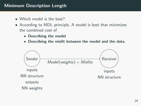
• Which model is the best?
• According to MDL principle, A model is best that minimizesthe combined cost of
• Describing the model
• Describing the misfit between the model and the data.
Sender
inputs
NN structure
outputs
NN weights
Receiver
inputs
NN structure
Model(weights) + Misfits
24
Shannon’s Coding Theorem
• Entropy definition: H(X ) =∑
x P(x)(−logP(x))
• Shannon’s Coding Theorem:
• N i.i.d. random variables each with entropy H(X ) can be
compressed into more than NH(X ) bits with negligible risk of
information loss, as N →∞.
• Conversely, if they are compressed into fewer than NH(X ) bits
it is virtually certain that information will be lost.
• According to this theorem, if a sender and a receiver have
agreed on a distribution P(x), then we can code the x using
− log P(x) bits.
25
Coding the Data Misfits and the Weights
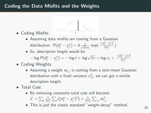
• Coding Misfits• Assuming data misfits are coming from a Gaussian
distribution: P(dcj − y c
j ) = t 1√2πσj
exp(−(dc
j −ycj )
2
2σ2j
)
• So, description length would be:
− log P(dcj − y c
j ) = − log t + log√
2π + log σj +−(dc
j −ycj )
2
2σ2j
• Coding Weights• Assuming a weight wi,j is coming from a zero-mean Gaussian
distribution with a fixed variance σ2w , we can get a similar
description length.
• Total Cost• By removing constants total cost will become:
C =∑
j1
2σ2j
∑c((dc
j − y cj )2) + 1
2σ2w
∑i,j w2
i,j
• This is just the classic standard ”weight-decay” method.26
Adding Noise to Weights
• More complicated problem can be obtained by adding
Gaussian noise to weights.
• Suppose sender and receiver have agreed on a Gaussian prior
P, for a given weight. After learning, the sender has a
Gaussian distribution, Q, for the weight.
P(w) : Normal
Q(w |D) = N(µw , σ2w )⇒ w = µw + ε, ε ∼ N(0, σ2w )
• Now, lets send the a noisy weight (model description) that
comes from posterior distribution by ”bits-back” coding
scheme.
27
Bits-back Argument
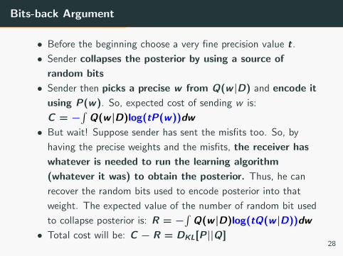
• Before the beginning choose a very fine precision value t.
• Sender collapses the posterior by using a source of
random bits
• Sender then picks a precise w from Q(w |D) and encode it
using P(w). So, expected cost of sending w is:
C = −∫
Q(w |D)log(tP(w))dw• But wait! Suppose sender has sent the misfits too. So, by
having the precise weights and the misfits, the receiver has
whatever is needed to run the learning algorithm
(whatever it was) to obtain the posterior. Thus, he can
recover the random bits used to encode posterior into that
weight. The expected value of the number of random bit used
to collapse posterior is: R = −∫
Q(w |D)log(tQ(w |D))dw• Total cost will be: C − R = DKL[P||Q]
28
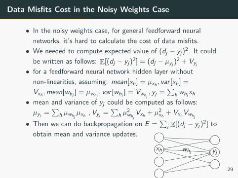
Data Misfits Cost in the Noisy Weights Case
• In the noisy weights case, for general feedforward neural
networks, it’s hard to calculate the cost of data misfits.
• We needed to compute expected value of (dj − yj)2. It could
be written as follows: E[(dj − yj)2] = (dj − µyj )2 + Vyj
• for a feedforward neural network hidden layer without
non-linearities, assuming: mean[xh] = µxh , var [xh] =
Vxh ,mean[whj ] = µwhj, var [whj ] = Vwhj
, yj =∑
h whj xh
• mean and variance of yj could be computed as follows:
µyj =∑
h µwhjµxh ,Vyj =
∑h µ
2whj
Vxh + µ2xh + VxhVwhj
• Then we can do backpropagation on E =∑
j E[(dj − yj)2] to
obtain mean and variance updates.
xh yjwhj
29
Hyper-priors, Other Priors
• Hyper-priors• So far, we have assumed the prior that is used for coding the
weights is a single Gaussian.
• In a Bayesian approach we set some hyper-parameters for the
parameters of the coding-prior. This would take into account
the cost of communicating coding-prior given hyper-priors. In
practice, we just ignore the cost of communicating the two
parameters of the coding-prior. This is in some sense similar to
type 2 maximum likelihood (marginalizing out the parameters):
arg maxα P(y |x , α) =∫
P(y |x ,w)P(w |α)dw
• More flexible prior• Gaussian prior is too limited to model many distributions on
weights in a feedforward neural network. Mixture of Gaussians
could be a good substitute. Why?
• Can model different structures.
• Could be useful when we want different coding-priors in
different subsets. 30

Practical VI for Neural Networks
Graves 2011
• Stochastic Variational Inference for Neural Networks
• Minimum description length (mdl)
• Approximate inference as Compression
• Optimisation
• Bayesian Formulation (vi) vs Coding Theory (mdl)
• Predictive Accuracy
• Generalization
• Model selection
• Occam’s Razor in Minimum message length (mml)
• Regularisation
31
Bayesian Formulation
• Variational free energy
F(α,β;D) =
⟨log
[qβ(w|D)
p(D|w)pα(w)
]⟩w∼qβ(w|D)
LN(w,D) = −log p(D|w)
• Evidence lower bound (elbo)
L(θ,φ; x) = Eqφ(z|x)[log pθ(x|z)
]− DKL(qφ(z|x)‖pθ(z))
• Equivalent formulations
L(θ,φ; x) = −F(θ,φ; x)
32
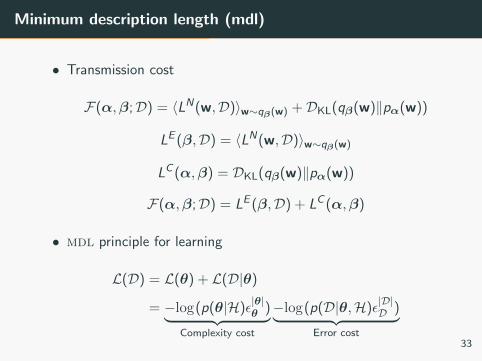
Minimum description length (mdl)
• Transmission cost
F(α,β;D) = 〈LN(w,D)〉w∼qβ(w) +DKL(qβ(w)‖pα(w))
LE (β,D) = 〈LN(w,D)〉w∼qβ(w)
LC (α,β) = DKL(qβ(w)‖pα(w))
F(α,β;D) = LE (β,D) + LC (α,β)
• mdl principle for learning
L(D) = L(θ) + L(D|θ)
= −log(p(θ|H)ε|θ|θ )︸ ︷︷ ︸
Complexity cost
−log(p(D|θ,H)ε|D|D )︸ ︷︷ ︸
Error cost33
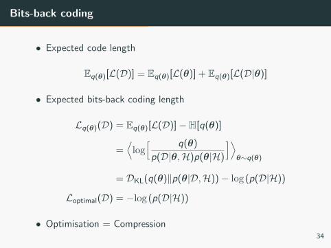
Bits-back coding
• Expected code length
Eq(θ)[L(D)] = Eq(θ)[L(θ)] + Eq(θ)[L(D|θ)]
• Expected bits-back coding length
Lq(θ)(D) = Eq(θ)[L(D)]−H[q(θ)]
=⟨log[ q(θ)
p(D|θ,H)p(θ|H)
]⟩θ∼q(θ)
= DKL(q(θ)‖p(θ|D,H))− log (p(D|H))
Loptimal(D) = −log (p(D|H))
• Optimisation = Compression34
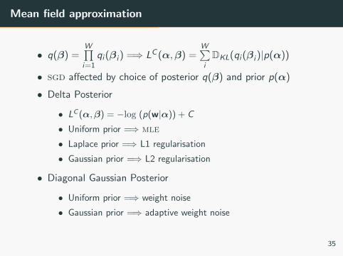
Mean field approximation
• q(β) =W∏i=1
qi (βi ) =⇒ LC (α,β) =W∑iDKL(qi (βi )|p(α))
• sgd affected by choice of posterior q(β) and prior p(α)
• Delta Posterior
• LC (α,β) = −log (p(w|α)) + C
• Uniform prior =⇒ mle
• Laplace prior =⇒ L1 regularisation
• Gaussian prior =⇒ L2 regularisation
• Diagonal Gaussian Posterior
• Uniform prior =⇒ weight noise
• Gaussian prior =⇒ adaptive weight noise
35
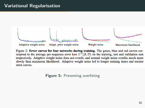
Variational Regularisation
Figure 5: Preventing overfitting
36
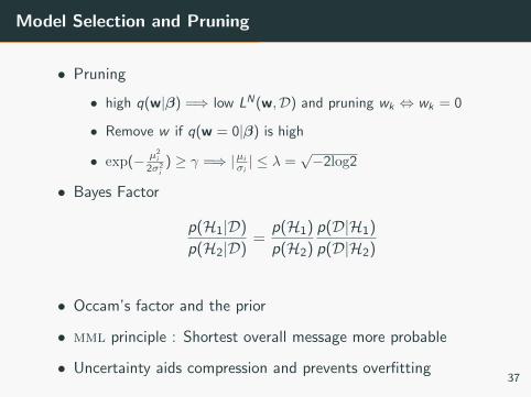
Model Selection and Pruning
• Pruning
• high q(w|β) =⇒ low LN(w,D) and pruning wk ⇔ wk = 0
• Remove w if q(w = 0|β) is high
• exp(− µ2i
2σ2i) ≥ γ =⇒ |µi
σi| ≤ λ =
√−2log2
• Bayes Factor
p(H1|D)
p(H2|D)=
p(H1)
p(H2)
p(D|H1)
p(D|H2)
• Occam’s factor and the prior
• mml principle : Shortest overall message more probable
• Uncertainty aids compression and prevents overfitting37
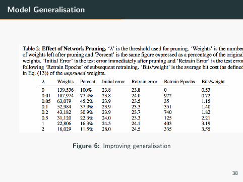
Model Generalisation
Figure 6: Improving generalisation
38
Weight Uncertainty in Neural Networks
Weight Uncertainty in Neural Networks
by Charles Blundell, Julien Cornebise, Koray Kavukcuoglu, and
Daan Wierstra
39
Problem Focused in the Work
• Utilize re-parametrization trick for limited amount of
parameters introduced through variational inference
• Formulate objective function to relax restrictions on prior and
variational posterior for requiring closed-form expression;
allowing more prior/variational posterior combinations
• Develop optimization algorithm for obtaining unbiased
gradient estimates, with small variances in gradient signals
40
Recap of Variational Inference
• Let P(w)|D) denote the actual posterior distribution on
weights provided with prior and data; Let q(w)|θ) denote
”variational posterior”: the distribution used to approximate
the actual posterior
• The essence of Variational Inference is to use Kullback-Leibler
divergence as the metric to obtain quality variational posterior
41
Mathematical Formulation for Optimization Problem
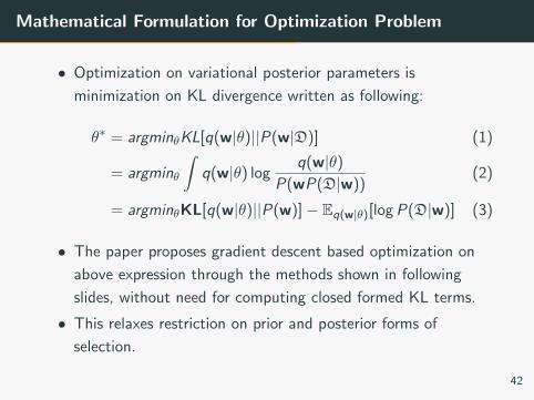
• Optimization on variational posterior parameters is
minimization on KL divergence written as following:
θ∗ = argminθKL[q(w|θ)||P(w|D)] (1)
= argminθ
∫q(w|θ) log
q(w|θ)
P(wP(D|w))(2)
= argminθKL[q(w|θ)||P(w)]− Eq(w|θ)[log P(D|w)] (3)
• The paper proposes gradient descent based optimization on
above expression through the methods shown in following
slides, without need for computing closed formed KL terms.
• This relaxes restriction on prior and posterior forms of
selection.
42
Defining the Objective Function for Optimization
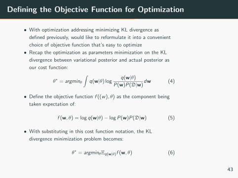
• With optimization addressing minimizing KL divergence as
defined previously, would like to reformulate it into a convenient
choice of objective function that’s easy to optimize
• Recap the optimization as parameters minimization on the KL
divergence between variational posterior and actual posterior as
our cost function:
θ∗ = argminθ
∫q(w|θ) log
q(w|θ)
P(w)P(D|w)dw (4)
• Define the objective function f ((w), θ) as the component being
taken expectation of:
f (w, θ) = log q(w|θ)− log P(w)P(D|w) (5)
• With substituting in this cost function notation, the KL
divergence minimization problem becomes:
θ∗ = argminθEq(w|θ)f (w, θ) (6)
43

Benefits for the Objective Function Choice
• With the objective function defined previously, a Monte Carlo
estimation is as following:
f (w, θ) ≈n∑
i=1
log q(w(i)|θ)− log P(w(i))− log P(D|w(i)) (7)
With weights samples w(i) drawn according to our variational
posterior• This formulation of objective function provides two computational
benefits:
1. Every term depends upon w(i) drawn from variational posterior, thus
utilizing a variance reduction technique common random numbers
(Owen, 2013) for the approximation.
2. Note that unlike original Variational Inference formulations
(maximizing ELBO):
ELBO = Ew q(w |θ)[log pθ(x |z)]− KL(q(w |θ)||p(z))︸ ︷︷ ︸complexity cost of the model
analytically computed for closed form term
(8)
This objective function doesn’t collect terms for getting this KL term,
and thus not requiring closed form solution to be computed. Thus this
allows richer prior/posterior combinations.
44
Optimization by Gradient Descent
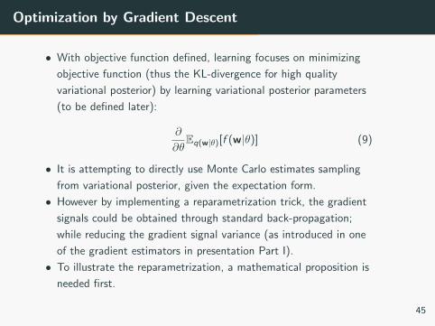
• With objective function defined, learning focuses on minimizing
objective function (thus the KL-divergence for high quality
variational posterior) by learning variational posterior parameters
(to be defined later):
∂
∂θEq(w|θ)[f (w|θ)] (9)
• It is attempting to directly use Monte Carlo estimates sampling
from variational posterior, given the expectation form.
• However by implementing a reparametrization trick, the gradient
signals could be obtained through standard back-propagation;
while reducing the gradient signal variance (as introduced in one
of the gradient estimators in presentation Part I).
• To illustrate the reparametrization, a mathematical proposition is
needed first.
45
An Important Mathematical Proposition
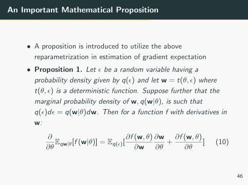
• A proposition is introduced to utilize the above
reparametrization in estimation of gradient expectation
• Proposition 1. Let ε be a random variable having a
probability density given by q(ε) and let w = t(θ, ε) where
t(θ, ε) is a deterministic function. Suppose further that the
marginal probability density of w, q(w|θ), is such that
q(ε)dε = q(w|θ)dw. Then for a function f with derivatives in
w:
∂
∂θEqw|θ[f (w|θ)] = Eq(ε)[
∂f (w, θ)
∂w
∂w
∂θ+∂f (w, θ)
∂θ] (10)
46
Reparametrization Trick on Variational Posterior
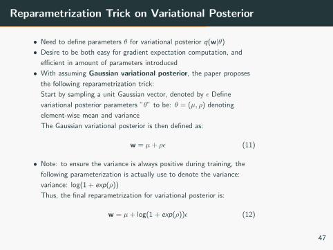
• Need to define parameters θ for variational posterior q(w|θ)
• Desire to be both easy for gradient expectation computation, and
efficient in amount of parameters introduced
• With assuming Gaussian variational posterior, the paper proposes
the following reparametrization trick:
Start by sampling a unit Gaussian vector, denoted by ε Define
variational posterior parameters ”θ” to be: θ = (µ, ρ) denoting
element-wise mean and variance
The Gaussian variational posterior is then defined as:
w = µ+ ρε (11)
• Note: to ensure the variance is always positive during training, the
following parameterization is actually use to denote the variance:
variance: log(1 + exp(ρ))
Thus, the final reparametrization for variational posterior is:
w = µ+ log(1 + exp(ρ))ε (12)
47
Optimize Network by Using Unbiased Monte Carlo Gradients
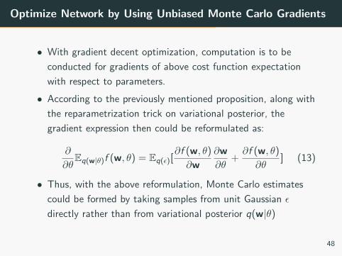
• With gradient decent optimization, computation is to be
conducted for gradients of above cost function expectation
with respect to parameters.
• According to the previously mentioned proposition, along with
the reparametrization trick on variational posterior, the
gradient expression then could be reformulated as:
∂
∂θEq(w|θ)f (w, θ) = Eq(ε)[
∂f (w, θ)
∂w
∂w
∂θ+∂f (w, θ)
∂θ] (13)
• Thus, with the above reformulation, Monte Carlo estimates
could be formed by taking samples from unit Gaussian ε
directly rather than from variational posterior q(w|θ)
48
Algorithm Steps for Optimization with Variational Inference on
Weights Posteriors
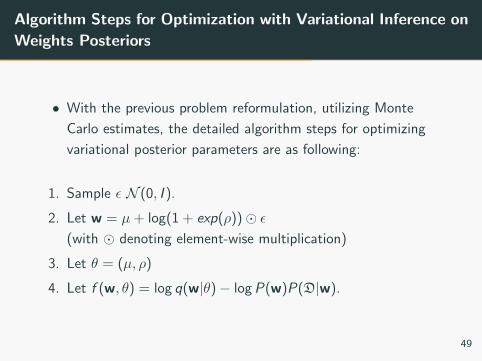
• With the previous problem reformulation, utilizing Monte
Carlo estimates, the detailed algorithm steps for optimizing
variational posterior parameters are as following:
1. Sample ε N (0, I ).
2. Let w = µ+ log(1 + exp(ρ))� ε(with � denoting element-wise multiplication)
3. Let θ = (µ, ρ)
4. Let f (w, θ) = log q(w|θ)− log P(w)P(D|w).
49
Continued: Algorithm Steps for Optimization with Variational
Inference on Weights Posteriors
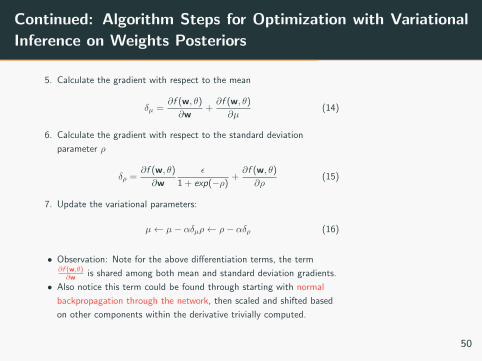
5. Calculate the gradient with respect to the mean
δµ =∂f (w, θ)
∂w+∂f (w, θ)
∂µ(14)
6. Calculate the gradient with respect to the standard deviation
parameter ρ
δρ =∂f (w, θ)
∂w
ε
1 + exp(−ρ)+∂f (w, θ)
∂ρ(15)
7. Update the variational parameters:
µ← µ− αδµρ← ρ− αδρ (16)
• Observation: Note for the above differentiation terms, the term∂f (w,θ)∂w is shared among both mean and standard deviation gradients.
• Also notice this term could be found through starting with normal
backpropagation through the network, then scaled and shifted based
on other components within the derivative trivially computed.
50
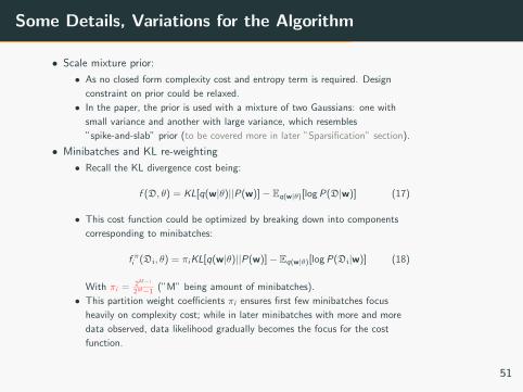
Some Details, Variations for the Algorithm
• Scale mixture prior:
• As no closed form complexity cost and entropy term is required. Design
constraint on prior could be relaxed.
• In the paper, the prior is used with a mixture of two Gaussians: one with
small variance and another with large variance, which resembles
”spike-and-slab” prior (to be covered more in later ”Sparsification” section).
• Minibatches and KL re-weighting
• Recall the KL divergence cost being:
f (D, θ) = KL[q(w|θ)||P(w)]− Eq(w|θ)[log P(D|w)] (17)
• This cost function could be optimized by breaking down into components
corresponding to minibatches:
f πi (Di, θ) = πiKL[q(w|θ)||P(w)]− Eq(w|θ)[log P(Di|w)] (18)
With πi = 2M−i
2M−1 (”M” being amount of minibatches).
• This partition weight coefficients πi ensures first few minibatches focus
heavily on complexity cost; while in later minibatches with more and more
data observed, data likelihood gradually becomes the focus for the cost
function.
51
Local Reparameterization Trick Variational Dropout and the
Local Reparameterization Trick
By Diederik P. Kingma, Tim Salimans, and Max Welling
52
Motivation
• If the variance in the gradients is too large, the stochastic
gradient ascent may not perform well.
• What’s the variance of the Stochastic Gradient Variational
Bayes (SGVB) estimator and how can we reduce it?
53
Variational Inference
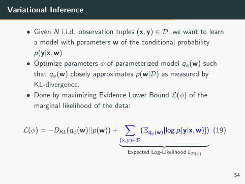
• Given N i.i.d. observation tuples (x, y) ∈ D, we want to learn
a model with parameters w of the conditional probability
p(y|x,w)
• Optimize parameters φ of parameterized model qφ(w) such
that qφ(w) closely approximates p(w|D) as measured by
KL-divergence.
• Done by maximizing Evidence Lower Bound L(φ) of the
marginal likelihood of the data:
L(φ) = −DKL(qφ(w)||p(w)) +∑
(x ,y)∈D
(Eqφ(w)[log p(y|x,w)])
︸ ︷︷ ︸Expected Log-Likelihood LD(φ)
(19)
54
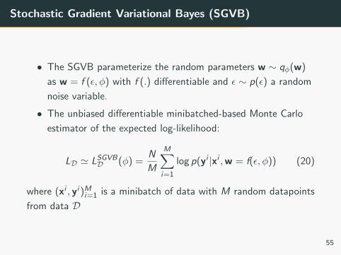
Stochastic Gradient Variational Bayes (SGVB)
• The SGVB parameterize the random parameters w ∼ qφ(w)
as w = f (ε, φ) with f (.) differentiable and ε ∼ p(ε) a random
noise variable.
• The unbiased differentiable minibatched-based Monte Carlo
estimator of the expected log-likelihood:
LD ' LSGVBD (φ) =
N
M
M∑i=1
log p(yi |xi ,w = f(ε, φ)) (20)
where (xi , yi )Mi=1 is a minibatch of data with M random datapoints
from data D
55
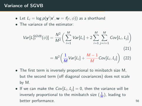
Variance of SGVB
• Let Li = log p(yi |xi ,w = f(ε, φ)) as a shorthand
• The variance of the estimator:
Var [LSGVBD (φ)] =
N2
M2
( M∑i=1
Var [Li ] + 2M∑i=1
M∑j=i+1
Cov [Li , Lj ]
)(21)
= N2
(1
MVar [Li ] +
M − 1
MCov [Li , Lj ]
)(22)
• The first term is inversely proportional to minibatch size M,
but the second term (off diagonal covariances) does not scale
by M.
• If we can make the Cov [Li , Lj ] = 0, then the variance will be
inversely proportional to the minibatch size ( 1M ), leading to
better performance. 56
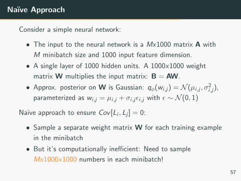
Naıve Approach
Consider a simple neural network:
• The input to the neural network is a Mx1000 matrix A with
M minibatch size and 1000 input feature dimension.
• A single layer of 1000 hidden units. A 1000x1000 weight
matrix W multiplies the input matrix: B = AW.
• Approx. posterior on W is Gaussian: qφ(wi ,j) = N (µi ,j , σ2i ,j),
parameterized as wi ,j = µi ,j + σi ,jεi ,j with ε ∼ N (0, 1)
Naıve approach to ensure Cov [Li , Lj ] = 0:
• Sample a separate weight matrix W for each training example
in the minibatch
• But it’s computationally inefficient: Need to sample
Mx1000x1000 numbers in each minibatch!
57
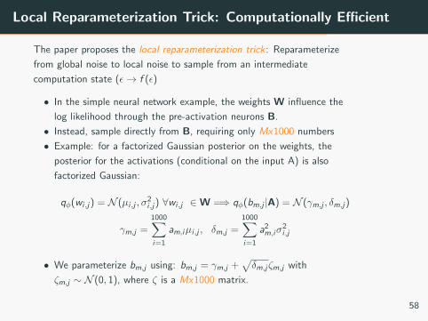
Local Reparameterization Trick: Computationally Efficient
The paper proposes the local reparameterization trick: Reparameterize
from global noise to local noise to sample from an intermediate
computation state (ε→ f (ε)
• In the simple neural network example, the weights W influence the
log likelihood through the pre-activation neurons B.
• Instead, sample directly from B, requiring only Mx1000 numbers
• Example: for a factorized Gaussian posterior on the weights, the
posterior for the activations (conditional on the input A) is also
factorized Gaussian:
qφ(wi ,j) = N (µi ,j , σ2i ,j) ∀wi ,j ∈W =⇒ qφ(bm,j |A) = N (γm,j , δm,j)
γm,j =1000∑i=1
am,iµi ,j , δm,j =1000∑i=1
a2m,iσ2i ,j
• We parameterize bm,j using: bm,j = γm,j +√δm,jζm,j with
ζm,j ∼ N (0, 1), where ζ is a Mx1000 matrix.
58
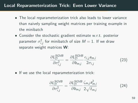
Local Reparameterization Trick: Even Lower Variance
• The local reparameterization trick also leads to lower variance
than naively sampling weight matrices per training example in
the minibatch
• Consider the stochastic gradient estimate w.r.t. posterior
parameter σ2i ,j for minibatch of size M = 1. If we draw
separate weight matrices W:
∂LSGVBD∂σ2i ,j
=∂LSGVBD
∂bm,j
εi ,jam,i2σi ,j
(23)
• If we use the local reparameterization trick:
∂LSGVBD∂σ2i ,j
=∂LSGVBD
∂bm,j
ζm,ja2m,i
2√δm,j
(24)
59
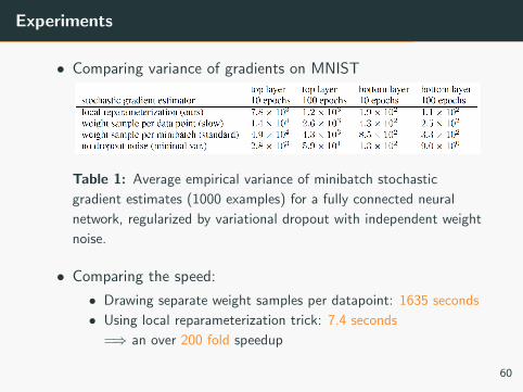
Experiments
• Comparing variance of gradients on MNIST
Table 1: Average empirical variance of minibatch stochastic
gradient estimates (1000 examples) for a fully connected neural
network, regularized by variational dropout with independent weight
noise.
• Comparing the speed:
• Drawing separate weight samples per datapoint: 1635 seconds
• Using local reparameterization trick: 7.4 seconds
=⇒ an over 200 fold speedup
60
Sparsification
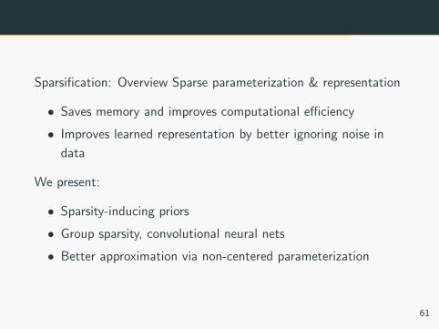
Sparsification: Overview Sparse parameterization & representation
• Saves memory and improves computational efficiency
• Improves learned representation by better ignoring noise in
data
We present:
• Sparsity-inducing priors
• Group sparsity, convolutional neural nets
• Better approximation via non-centered parameterization
61
Sparsity-inducing priors
• p(w |D) ∝ p(D|w)p(w) =⇒ structure of prior could affect
posterior
• What kind of priors could encourage sparsity:
• Having a mean/mode at zero?
• Having a lot of density near zero?
• Neither are sufficient as eg. a N (0, σ2) prior only squashes
weights.
62
Sparsity-inducing priors
• p(w |D) ∝ p(D|w)p(w) =⇒ structure of prior could affect
posterior
• What kind of priors could encourage sparsity:
• Having a mean/mode at zero?
• Having a lot of density near zero?
• Neither are sufficient as eg. a N (0, σ2) prior only squashes
weights.
62
Spike and slab priors
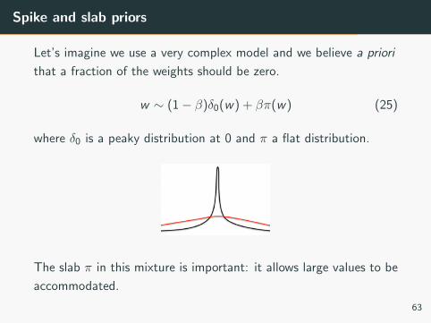
Let’s imagine we use a very complex model and we believe a priori
that a fraction of the weights should be zero.
w ∼ (1− β)δ0(w) + βπ(w) (25)
where δ0 is a peaky distribution at 0 and π a flat distribution.
The slab π in this mixture is important: it allows large values to be
accommodated.
63
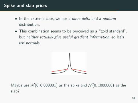
Spike and slab priors
• In the extreme case, we use a dirac delta and a uniform
distribution.
• This combination seems to be perceived as a “gold standard”,
but neither actually give useful gradient information, so let’s
use normals.
Maybe use N (0, 0.000001) as the spike and N (0, 1000000) as the
slab?
64
Scale mixture of normals
Instead of a finite mixture, we can take an infinite one. Define:
(w |λ) ∼ N (w |0, λ2), λ ∼ p(λ) (26)
The marginal distribution of w (integrating λ out) is the mixture
of various normal distributions that are centered at zero with
different scales
p(w) =
∫p(λ)N (w |0, λ2)dλ (27)
65
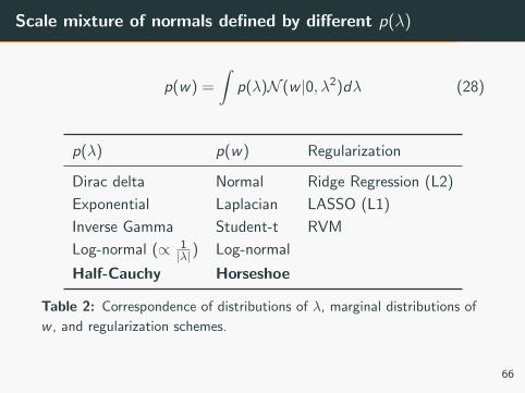
Scale mixture of normals defined by different p(λ)
p(w) =
∫p(λ)N (w |0, λ2)dλ (28)
p(λ) p(w) Regularization
Dirac delta Normal Ridge Regression (L2)
Exponential Laplacian LASSO (L1)
Inverse Gamma Student-t RVM
Log-normal (∝ 1|λ|) Log-normal
Half-Cauchy Horseshoe
Table 2: Correspondence of distributions of λ, marginal distributions of
w , and regularization schemes.
66
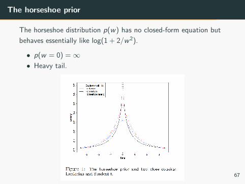
The horseshoe prior
The horseshoe distribution p(w) has no closed-form equation but
behaves essentially like log(1 + 2/w2).
• p(w = 0) =∞• Heavy tail.
67
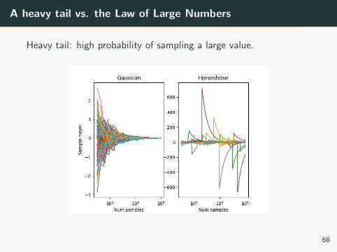
A heavy tail vs. the Law of Large Numbers
Heavy tail: high probability of sampling a large value.
68
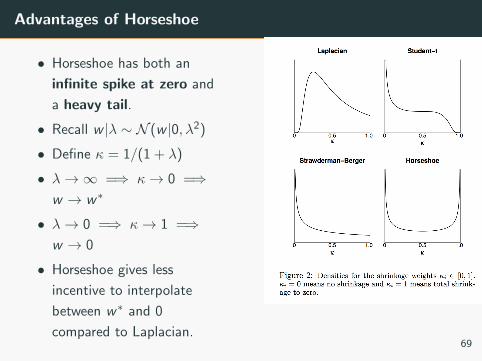
Advantages of Horseshoe
• Horseshoe has both an
infinite spike at zero and
a heavy tail.
• Recall w |λ ∼ N (w |0, λ2)
• Define κ = 1/(1 + λ)
• λ→∞ =⇒ κ→ 0 =⇒w → w∗
• λ→ 0 =⇒ κ→ 1 =⇒w → 0
• Horseshoe gives less
incentive to interpolate
between w∗ and 0
compared to Laplacian.69
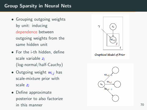
Group Sparsity in Neural Nets
• Grouping outgoing weights
by unit: inducing
dependence between
outgoing weights from the
same hidden unit
• For the i-th hidden, define
scale variable zi
(log-normal/half-Cauchy)
• Outgoing weight wi ,j has
scale-mixture prior with
scale zi
• Define approximate
posterior to also factorize
in this manner 70
Group Sparsity in Neural Nets
What we need for VI to work:
• Efficient Sampling from approximate posterior
• Achieved by ancestral sampling. Sample zi from q(zi ), then
sample wi,j from q(wi,j |zi )• Evaluating the KL(q(W ,Z )||p(W ,Z ))
• Eq(Z)[KL(q(W |Z )||p(W |Z ))] + KL(q(Z )||p(Z ))
• KL(q(W |Z )||p(W |Z )) can be computed in closed form when
q(W |Z ) and p(W |Z ) are Gaussians
• KL(q(Z )||p(Z )) can be computed in closed form when both
q(Z ) and p(Z ) are Gaussian OR q(Z ) is half-Cauchy and p(Z )
is log-normal
• Differentiability w.r.t. variational parameters is guaranteed
71
Group Sparsity in Neural Nets
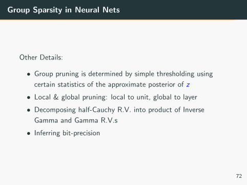
Other Details:
• Group pruning is determined by simple thresholding using
certain statistics of the approximate posterior of z
• Local & global pruning: local to unit, global to layer
• Decomposing half-Cauchy R.V. into product of Inverse
Gamma and Gamma R.V.s
• Inferring bit-precision
72
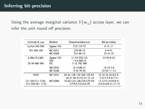
Inferring bit-precision
Using the average marginal variance V(wi ,j) across layer, we can
infer the unit round off precision.
73
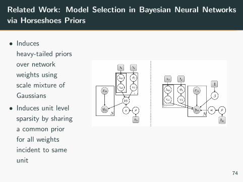
Related Work: Model Selection in Bayesian Neural Networks
via Horseshoes Priors
• Induces
heavy-tailed priors
over network
weights using
scale mixture of
Gaussians
• Induces unit level
sparsity by sharing
a common prior
for all weights
incident to same
unit
74
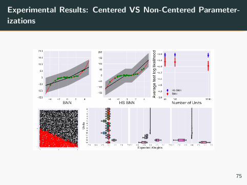
Experimental Results: Centered VS Non-Centered Parameter-
izations
75
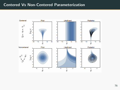
Centered Vs Non-Centered Parameterization
76
J. Ingraham and D. Marks, “Variational inference for sparse
and undirected models,” in Proceedings of the 34th
International Conference on Machine Learning (D. Precup and
Y. W. Teh, eds.), vol. 70 of Proceedings of Machine Learning
Research, (International Convention Centre, Sydney,
Australia), pp. 1607–1616, PMLR, 06–11 Aug 2017.
S. Ghosh and F. Doshi-Velez, “Model Selection in Bayesian
Neural Networks via Horseshoe Priors,” ArXiv e-prints, May
2017.
C. Louizos, K. Ullrich, and M. Welling, “Bayesian Compression
for Deep Learning,” ArXiv e-prints, May 2017.
C. M. Carvalho, N. G. Polson, and J. G. Scott, “Handling
sparsity via the horseshoe,” in Proceedings of the Twelth
International Conference on Artificial Intelligence and
76
Statistics (D. van Dyk and M. Welling, eds.), vol. 5 of
Proceedings of Machine Learning Research, (Hilton Clearwater
Beach Resort, Clearwater Beach, Florida USA), pp. 73–80,
PMLR, 16–18 Apr 2009.
76