Variation Dirichlet Blur Kernel Estimation doubledecsai.ugr.es/vip/files/journals/Variation...

JOURNAL OF LATEX CLASS FILES, VOL. 11, NO. 4, DECEMBER 2012 1

Variational Dirichlet Blur Kernel EstimationXu Zhou, Student Member, IEEE, Javier Mateos, Member, IEEE, Fugen Zhou, Member, IEEE,

Rafael Molina, Member, IEEE, and Aggelos K. Katsaggelos Fellow, IEEE

Abstract—Blind image deconvolution involves two key ob-jectives, latent image and blur estimation. For latent imageestimation, we propose a fast deconvolution algorithm, whichuses an image prior of nondimensional Gaussianity measureto enforce sparsity and an undetermined boundary conditionmethodology to reduce boundary artifacts. For blur estimation,a linear inverse problem with normalization and nonnegativeconstraints must be solved. However, the normalization constraintis ignored in many blind image deblurring methods, mainlybecause it makes the problem less tractable. In this paper, weshow that the normalization constraint can be very naturallyincorporated into the estimation process by using a Dirichletdistribution to approximate the posterior distribution of theblur. Making use of variational Dirichlet approximation, weprovide a blur posterior approximation that takes into accountthe uncertainty of the estimate and removes noise in the estimatedkernel. Experiments with synthetic and real data demonstratethat the proposed method is very competitive to state-of-the-artblind image restoration methods.

Index Terms—Blind Deconvolution, image deblurring, varia-tional distribution approximations, Dirichlet distribution, con-strained optimization, point spread function, inverse problem.

I. INTRODUCTION

BLIND image deconvolution (BID) refers to the problemof recovering the source image from a degraded obser-

vation when the blur kernel is unknown, using partial infor-mation about the imaging system [1]. Primary applicationsof BID include astronomical imaging, medical imaging, andcomputational photography [2].

Mathematically, the degraded observation y ∈ �M can beapproximately modeled as [2]

y = Hx+ n (1)

where x ∈ �N is the original image, H of size M ×N is theconvolution matrix whose row elements are obtained from theblur kernel h ∈ �K , and n ∈ �M is assumed to be additivezero-mean Gaussian white noise. BID is a severely ill-posedinverse problem, since multiple pairs of kernels and original

This work was sponsored in part by National Natural Science Foundationof China (61233005), Ministerio de Ciencia e Innovacion under ContractTIN2013-43880-R, the European Regional Development Fund (FEDER), theCEI BioTic with the Universidad de Granada and the Department of Energygrant DE-NA0002520.

X. Zhou and F. Zhou are with the Image Processing Center, Bei-hang University, Beijing 100191, China (e-mail: [email protected]; [email protected]). X. Zhou performed the work while at Universidad deGranada, as a joint-PhD student sponsored by Chinese Scholarship Council.

J. Mateos and R. Molina are with Departamento de Ciencias de laComputacion e I.A., Universidad de Granada, Granada 18071, Spain (e-mail:[email protected]; [email protected]).

A. Katsaggelos is with the Department of Electrical Engineering andComputer Science, Northwestern University, Evanston, IL 60208-3118 USA(e-mail: [email protected]).

images can match the model (1) equally well. To overcome theill-posed nature of BID, additional constraints or assumptionson both x and h must be introduced.

Many earlier works assume that the blur kernel followsa parametric model [1] [2] or satisfies some additional con-straints, e.g., centrosymmetric, nonnegative and normalizationconstraint [3] [4]. For the latent image, many BID methods[5]–[23] utilize image sparsity to estimate the image.

Fergus et al. [5] assume that the gradient of the latentimage ∇x obeys a heavy-tailed distribution, meaning thatmost elements of ∇x are zero or very small but a numberof elements are quite large. Specifically, they use a Mixture ofGaussians (MoG) to approximate a heavy-tailed distribution.However, as pointed out in [5], [24], and [17], using themaximum a posteriori (MAP) approach often yields deltakernels because the cost function favors a blurry explana-tion over sharp reconstructions. To avoid this problem, theVariational Bayesian (VB) approach [25] has been adoptedin [5], see also [26] [27] [17]. Using the VB approach, ageneral framework based on the Super Gaussian priors isproposed by Babacan et al. [17]. Instead of using MAPestimation, Levin et al. [24] [11] suggest a MAPh approach,namely marginalizing over latent images and then estimatingthe kernel alone. The rationale behind MAPh is that estimatingh alone is much better conditioned than estimating h and xtogether. Recently, following the MAPh approach and usinga majorization-minimization approach, Zhang and Wipf [23]propose a parameter free BID method for removing camerashake, in which the gradient image is modeled by an inde-pendent Gaussian distribution with zero mean and spatiallyvarying variance. Interested readers are referred to [28] for areview of of Bayesian blind deconvolution methods.

An alternative to enforce image sparsity in the transformdomain is to use the shock filter [29], see [7] and [9]. In fact,the shock filter not only promotes image sparsity, but alsopredicts step edges. Following this idea, Xu and Jia [14] pointout that not all predicted step edges are helpful. Therefore, theysuggest an edge selection strategy for removing texture edges,which improves the result significantly. Instead of predictingstep edges, a probably better idea is to model step edgesas local minima of a sparsity measure, e.g., ‖∇x‖1/‖∇x‖2,‖∇x‖0,

∑i |∇x(i)|/(|∇x(i)|+‖∇x‖1/N), see [12], [15] and

[22] for more details. Sun et al. [19] also propose a novelparameterized patch model to regularize step edges, usinglearned image statistics or synthetic structures. Making use ofdirectional filters, Zhong et al. [20] show that a good kernelcan be estimated from a blurred image with 1%− 10% noise.Step edge based methods are robust to noise since noise andsmall gradients are smoothed out, but may fail if the image isdominated by textures. By combining step edge prediction [9]


with covariance image [11] used in kernel estimation, Wanget al [18] propose a robust BID method.

In this work, a BID algorithm that alternates between theestimation of image and blur is proposed. For the latent imageestimation, we use the Nondimensional Gaussianity Measure(NGM) proposed in [22], to promote image sparsity. As theoptimization algorithm of [22] does not make use of the FFT,we propose a fast deconvolution algorithm with undeterminedboundary condition [30] to estimate the latent sharp image,which uses the variable splitting [31] and mask decoupling[32] [33] approaches. For the blur estimation part we proposea Variational Dirichlet (VD) method. This changes the regular-ization based approach to a variational Bayes approximationto estimate the posterior distribution of the blur. The benefit ofusing VD is that the resulting optimization problem does nothave any equality constraint but lower bound constraints only,so that it can be efficiently solved by the gradient projectionmethod [34]. The other benefit of VD is a new adaptivesparsity promoting term associated with the image, which ishelpful to remove the kernel noise. Furthermore as we willlater show, the VD approach can be applied to regularizationand variational based BID methods that alternate betweenimage and blur estimation, where the blur energy function(either from regularization or blur prior) is quadratic. This isthe case of many state-of-the-art BID methods. In summary,the main contributions of this paper include a novel efficientoptimization algorithm in the image space for NGM baseddeconvolution and a novel VD approach for kernel estimation.

This paper is organized as follows. In Section II, weintroduce the framework to be used in BID. In Section III,we propose a fast nonblind image deconvolution algorithmformulated in the image domain for the NGM model in [22].Section IV contains our blur kernel estimation algorithm.We derive the VD approximation and show the connectionbetween VD approximation and MAP estimation. An efficientgradient projection algorithm is proposed to solve the resultingoptimization problem. This section also discusses the appli-cations of the proposed VD in kernel estimation when theblur prior is quadratic. A multiscale implementation of the VDbased BID method is presented in Section IV-D, followed by adiscussion on parameter setting and implementation in SectionIV-E. In Section V, we compare our BID method with state-of-the-art BID methods. Experimental results on synthetic andreal data show that the proposed method is very competitivein comparison with state-of-the-art BID algorithms [15], [17],[19], [20]. Finally, Section VI concludes this paper.

II. REGULARIZATION BASED BLIND IMAGEDECONVOLUTION

Regularization based BID methods, [3], [4], [7], [10], [21],[26], [27], just to name a few, alternatively solve the followingtwo optimization problems,

xk+1 = argminx

1

2‖Hkx− y‖22 + λxRx(x), (2)

hk+1 = argminh

1

2‖Xk+1h− y‖22 +

λh

2Rh(h), (3)

subject to h ≥ 0 (4)∑j

h(j) = 1 (5)

where k denotes iteration index, Hk is the convolution matrixformed by the estimated impulse response of the blur at thek-th iteration step hk, Xk+1 is the convolution matrix formedby the restored image xk+1, Rx and Rh are regularizationfunctions, λx > 0 and λh ≥ 0 are penalty weights controllingthe tradeoff between the data fitting term and regularization.

Recent published papers, see for instance [9], [11], [15],[17] have shown, however, that using gradient images leads tobetter kernel estimation. Furthermore, the final output imageof (2) is often highly smoothed mainly due to the largepenalty weight λx, which is not a desirable result. After kernelestimation, to reconstruct the final sharp image a nonblindimage deconvolution method is required.

In this work we replace the blur estimation problem definedin (3)-(5) by the filter space formulation

hk+1 = argminh

∑i

1

2‖∇iX

k+1h−∇iy‖22 +λh

2Rh(h),(6)

subject to h ≥ 0 (7)∑j

h(j) = 1 (8)

where now ∇iXk+1 is the matrix formed by the gradient of

the image xk+1 utilizing the i-th filter (details on the filtersused will be provided later).

Note that we are formulating the image estimation in thespatial domain and the blur estimation in the gradient domain.Xu et al. [15] indicate that using this spatial/filter formulationis better than using the same space formulation. One of themerits of using the gradient domain for kernel estimation isthat the boundary artifacts are reduced significantly since mostof the gradients at the boundaries are zero. This spatial/filterformulation prevents us from using the same cost function tobe minimized on the image and blur and consequently makesit harder to establish the convergence of the iterative method,however, as we will show in the experimental section this dualformulation produces better image and blur estimates.

The above framework has two steps, namely, the latentimage estimation step according to (2) with a given h, andthe kernel estimation step according to (6)-(8) with a givenx. By alternatively solving (2) and (6)-(8), one obtains agood estimation of the kernel, provided that a good imageregularization Rx(x) and a good kernel regularization Rh(h)are used. It should be noted that both Rx(x) and Rh(h)might evolve during the iterations (e.g., edge-predicting basedmethod [9] and VB method [17]).

When the uncertainty of the image and blur are not tak-en into account and Rx(x) and Rh(h) do not incorporateinformation on the covariance of x and h respectively, thisiterative framework is also known as MAP approach in theBayesian formulation. It may not work well depending on the


initialization of the kernel, images priors/regularizations andkernel priors/regularizations. As shown in Levin et al. [24], theMAP approach may suffer from the delta kernel in the caseof lp regularization (Rx(x) =

∑j |∇x(j)|p with p ∈ (0, 2]),

since the cost function favors no-blur explanation (h is thedelta kernel and x = y) over other solutions.

III. FAST IMAGE DECONVOLUTION USING NGM

Let us now proceed with the solution of problem (2), thatis, the image estimation part. Let us assume that we have ablur estimation and face the problem of estimating the latentimage from the blurred observation.

In [22], to enforce sparsity, we proposed a NondimensionalGaussianity Measure (NGM),

∑2i=1

∑j |∇ix(j)|/(|∇ix(j)|+

E[|∇ix|]), where i = 1 and 2 denote horizontal and verticalfiltering respectively and E[|∇ix|] denotes the mean value ofthe vector |∇ix|, see [22] for details.

Decreasing NGM concentrates the energy at a small numberof elements with most of them being zero or very small values.In other words, NGM favors sharp step edges over blurry ones.An example of a 3-D NGM is shown in Fig. 1.

For a given kernel h, we propose here to estimate a sharpimage as the minimizer of

minx

1

2‖Hx− y‖22 + λx

2∑i=1

∑j

|∇ix(j)||∇ix(j)|+ E[|∇ix|] (9)

where λx > 0 is a penalty weight that controls the degree ofsparsity. This model differs from the one in [22], since theimage estimation step in [22] (Eq. (7)) is formulated in thegradient domain.

To mitigate boundary artifacts, we adopt here undeterminedboundary conditions [30] (see [35] for other boundary condi-tions). That is to say, H = MpTh, where Mp is an M × Nmatrix that extracts the Field of View (FOV) of image x and Th

is an N×N circulant matrix that performs circular convolutionwith kernel h (see [32], [33] and [35] for more details).

Making use of variable splitting [31] and mask decoupling[32], [33], we show how (9) can be solved efficiently. Asin [32], [33] and [31], we introduce two auxiliary variablesu = Thx and v = ∇x (specifically, vi = ∇ix). Usingthe augmented Lagrangian and penalty approach for the con-straints u = Thx and v = ∇x, respectively, we obtain theunconstrained problem

minx,u,v

1

2‖Mpu− y‖22 +

λu

2‖u− Thx− du‖22

+2∑

i=1

λv

2‖vi −∇ix‖22 + λx

∑j

|vi(j)||vi(j)|+ E[|vi|] , (10)

where λu and λv are the penalty weights and du is theLagrangian multiplier. To obtain a good approximate solutionto problem (9), λv has to be very large. In practice, a largepenalty weight makes the algorithm very inefficient, so acontinuous strategy, like the one in [31], is adopted for thepenalty weight λv . We use an alternative minimization scheme,namely minimizing over one variable with the other two fixed.Consequently, we have to solve three subproblems as follows.

Fig. 1. 3-D NGM = xx+1/3

+ yy+1/3

+ 1−x−y1−x−y+1/3

. It is clear thatminimizing NGM pushes (x, y, 1− x− y) away from (1/3, 1/3, 1/3) andmakes it more sparse, namely the third component increases while the othertwo decrease.

A. u-subproblem

Given x, du, and v, we need to solve

minu

1

2‖Mpu− y‖22 +

λu

2‖u− Thx− du‖22, (11)

Clearly, problem (11) has a closed form solution, given by

u = (MTp Mp + λuI)

−1(MTp y + λu(Thx+ du)), (12)

where MTp pads y to an image of size N with zeros in both

dimensions. Note that MTp Mp is a diagonal matrix and hence,

the inversion (MTp Mp + λuI)

−1 is trivial.After updating u, we update du by

du = du+ Thx− u. (13)

B. x-subproblem

Given u, du and v, we need to solve

minx

λu

2‖u− Thx− du‖22 +

2∑i=1

λv

2‖vi −∇ix‖22. (14)

Again, this problem also has a closed form solution. Assumingperiodic boundary conditions for ∇i, the solution can beefficiently computed with the use of a 2-D FFT.

C. v-subproblem

Given x, du, and u, we need to solve

minvi

=λv

2‖vi −∇ix‖22 + λx

∑j

|vi(j)||vi(j)|+ E[|vi|] , (15)

where i = 1, 2. The above cost function is nonconvex andinseparable. However, if we fix E[|vi|] from the previousiteration, it can be simplified as a single variable minimizationproblem, given by

minz

g(z) =1

2‖z − w‖22 + λ

|z||z|+ E

, (16)

where λ = λx

λv, E = E[|vi|] and w represents a component of

∇ix. Note that the minimizer z∗ must have the same sign as w,


Algorithm 1 Fast NGM DeconvolutionRequire: y, x0, λx, λu, λv .

1: precompute the Fourier transform of h, ∇1 and ∇2

2: u = MTp y, x = x0, du = 0

3: repeat4: update u using (12)5: update du using (13)6: vi = ∇ix, si = sign(∇ix), i = 1, 27: for j = 1 to 2 do8: Ei = mean(|vi|), i = 1, 29: vi = si max(|∇ix| − λxEi

λv(|vi|+Ei)2, 0), i = 1, 2

10: end for11: λv = min(λv

√2, 1)

12: update x by solving (14) in Fourier domain13: until convergence14: return x

since replacing z by zs = sign(w)|z| we have g(z) ≥ g(zs).Let us examine the case w ≥ 0, we aim at finding

minz≥0

g(z) =1

2‖z − w‖22 + λ

z

z + E. (17)

Letting g′(z) = 0, we have

z = max(w − λE

(z + E)2, 0) (18)

This equation implies a fixed point iteration formula zt+1 =max(w − λE/(zt + E)2, 0). Together with the case w < 0,we have the ultimate fixed point iteration for (16)

zt+1 = sign(w)max(|w| − λE

(|zt|+ E)2, 0), t = 0, 1, 2...

(19)The iterative formula (19) implies |z∗| ≤ |w|, which guidesus to use z0 = w. Noting that |w| − λE/(|z|+ E)2 ismonotonically decreasing as |z| decreases, it can be shownthat the sequence {zt} generated by (19) with the initializationz0 = w is also monotonic, and it converges to a stationarypoint of g or zero. We observe that only two iterations areusually needed to obtain a good approximate solution.

Equation (19) can be viewed as a shrinkage operator, sinceit always moves the input towards zero. Unlike the shrinkageoperator in (10) of [22], it has a new spatially variant thresholdthat better preserves edge and promotes smoothness. Moreimportantly, we fix only a scalar E[|vi|] in each inner iteration,whereas in [22] the whole denominator |vi|+E[|vi|] is fixed,which probably alters the properties of NGM.

D. AlgorithmThe alternating minimization algorithm for (10) is presented

in Alg. 1 which achieves state-of-the-art speed, since theupdates for u and v are element-wise operations and the x-update can be efficiently implemented using a 2-D FFT. Thepenalty weight λu is set to 0.1, more choices can be foundin [32], and λv is set initially to a small value, i.e., 0.001.Since the mean value E[|vi|] is not a constant in the wholeiterative process, we can not prove the convergence of Alg. 1theoretically, but we show its convergence empirically in theexperimental section.

IV. VARIATIONAL DIRICHLET

In this section, we approach the solution of (6) withconstraints (7) and (8) using variational inference, under theassumption that Rh(h) = hTQh with Q being a K × Ksemidefinite symmetric matrix. This is a regularization modelfrequently found in the BID literature where, for instance,Rh(h) takes into account the covariance matrix of the imageestimate (see Levin et al. [11] and Babacan et al. [17]).

The solution of (6) without considering the constraints in (7)and (8) can be rewritten as a quadratic optimization problem(for simplicity, the iteration index is removed),

h∗ = argmaxh

fx(h) ≡ 1

2hTAh+ bTh (20)

where

A =2∑

i=1

∇iXT∇iX + λhQ (21)

b = −2∑

i=1

∇iXT∇iy (22)

The cost function fx(h) can be derived from the MAPapproach, for the Gaussian conditional probability p(y|h) ∝e−

∑2

i=1

12‖∇iXh−∇iy‖2

2 and the blur Gaussian prior p(h) ∝e−

λh2 hTQh. A shortcoming of the MAP approach is that the

constraints (7) and (8) cannot be integrated with the costfunction.

The Variational Dirichlet approach we are about to proposeaims at approximating the solution in (20) by finding a Dirich-let distribution that is the closest one, in the Kullback−Leibler(KL) divergence sense, to the posterior distribution of theblur given the observation. The Dirichlet distribution generatesvalues always greater than zero, with their sum equal toone. The use of the Dirichlet distribution incorporates in anatural way the constraints in (7) and (8) without the need toexplicitly include them into the problem. The parameters ofthe distribution indicate how sparse the obtained solution willbe.

Let S = {h|hi > 0, i = 1, 2, ...K,∑

i hi = 1} be theK−1 dimensional simplex and qα(h) the Dirichlet probabilitydensity function (see p. 261 in [36]), defined as

qα(h) =1

B(α)

K∏i=1

hαi−1i , (h ∈ S andαi > 0), (23)

where B(α) is called the multinomial Beta function and hasthe form

B(α) =

∏Ki=1 Γ(αi)

Γ(Sα), (24)

with Γ denoting the gamma function and Sα =∑K

i=1 αi.Then, we aim at finding the Dirichlet distribution

qα(h) = arg minqα∈Ω

KL(qα(h), p(h|y)) (25)

where Ω denotes the set of Dirichlet distribution in (23)with α = (α1, ..., αK) and all its components greater than


a lower bound lb > 0. This is equivalent to finding a factor αsatisfying

α = arg minα≥lb

KL(qα(h), p(h|y))

= arg minα≥lb

∫S

qα(h) logqα(h)

p(h|y)dh

= arg minα≥lb

∫S

qα(h) logqα(h)

p(y|h)p(h)dh

= arg minα≥lb

∫S

qα(h) logqα(h)

e−12h

TAh−bThdh

= arg minα≥lb

Eqα [log qα(h)] +1

2Eqα [h

TAh] + Eqα [bTh] (26)

where α ≥ lb should be understood as α having all itscomponents greater or equal to lb. Theoretically, α > 0 isadequate. However, in practice, we need a lower bound for αto avoid numerical instability.

After finding a solution α to (26), one can use the ex-pectation α/Sα as an estimation of the kernel. However,preliminary experiments show that model (26) always leadsto very poor kernel estimation. Such failures, as we will showsoon, are indeed caused by the over-weighted negentropy termEqα [log qα(h)]. To avoid this problem, we introduce a weightγ on this term. As a result, we obtain a more general model

arg minα≥lb

γEqα [log qα(h)] +1

2Eqα [h

TAh] + Eqα [bTh], (27)

which includes (26) as a special case when γ = 1.The rationale behind the introduction of γ is the following.

Eq. (27) is equivalent to minimizing KL(qα(h), pγ(h|y))where pγ(h|y)) ∝ e−

∑2

i=1

12γ ‖∇iXh−∇iy‖2

2−λh2γ hTQh. By

making γ small we approach a degenerate posterior distribu-tion on h, pγ(h|y). So qα(h) minimizing (27) will provide aDirichlet approximation to a neighbour of the MAP. Further-more, since we are minimizing the reverse KL, also knownas I-projection or information projection (see [37] for details),where pγ(h|y) is small qα(h) will also have to be small.

As shown in [36], the negentropy term has the form

Eqα [log qα(h)] = (α− 1)T (ψ(α)− ψ(Sα)1)− log(B(α)),(28)

where ψ = Γ′/Γ is the digamma function. Making use ofthe expectation Eqα(h)[h] = α/Sα and covariance matrix Σα

given in [36], we obtain in a straightforward way

Eqα [hTAh]=Tr(AΣα) + Eqα(h)[h]

TAEqα(h)[h]

=SαA

Td α− αTAα

S2α(Sα + 1)

+αTAα

S2α

=αTAα+AT

d α

(Sα + 1)Sα, (29)

Eqα [bTh]=

αT b

Sα, (30)

where Ad is the vector formed with the diagonal elements ofA, i.e., Ad(i) = Aii, i = 1, 2, ...K. Together with (28), (29)

and (30), the cost function in (27) has the following form

L(α) = γ[(α− 1)T (ψ(α)− ψ(Sα)1)− log(B(α))]

+αTAα+AT

d α

2(Sα + 1)Sα+

bTα

Sα, (31)

whose gradient is

∇L(α) = γ(α− 1) ◦ (ψ′(α)− ψ′(Sα)1) +2Aα+Ad

2(Sα + 1)Sα

+b

Sα− (αTAα+AT

d α)(2Sα + 1)

2(Sα + 1)2S2α

− bTα

S2α

, (32)

where ◦ denotes element-wise product.Before showing how to optimize L(α), let us discuss the

connection between γ and Sα. As γ goes to zero, pγ(h|y)becomes degenerate and hence, pα will also have to be closeto a degenerate distribution. For a Dirichlet distribution to bedegenerate, we need Sα to be infinity. The larger the value ofSα, the closer we are to the MAP solution and therefore thesmaller the approximation of the distribution around the MAP.As we will see in the experimental section, approximating thedistribution around the MAP rather than finding the MAP leadsto reduced noise in the estimated kernel.

L(α) has three terms, the negentropy, quadratic and linearterms. Notice that, since ψ′(α) is strictly decreasing, thenegentropy term has a unique stationary point α = 1 and,hence, favors the uniform distribution, namely q(h) = const.Consequently, decreasing the negentropy term will push αto the point 1. AT

d α in the quadratic term can be viewas a weighted l1 term while AT

d α2(Sα+1)Sα

adaptively promotessparsity. Since the weights in Ad are formed from ∇iX

T∇iXand Q, sparsity is promoted adaptively regardless of the scaleof ∇iX

T∇iX . Of course, if Sα goes to infinity, this term willvanish. αTAα

2(Sα+1)Sα+ bTα

Sαcan be viewed as the data fidelity

term with regularization Rh.The benefit of the new model is twofold. On one hand, it has

an adaptive sparsity regularization term, which can be usefulin sparse kernel estimation. On the other hand, it does nothave the equality constraint, which allows the optimizationproblem to be efficiently solved by the gradient projectionmethod [34]. Note that, with the equality constraint, we cannot use the gradient projection method. As a disadvantage, thecost function becomes nonconvex.

A. Optimization Algorithm

Let us minimize L(α) with lower bound constraint α ≥ lb.As L(α) is nonconvex, we search for a local minimum. Withthe gradient ∇L(α) defined in (32) at hand, we can use thegradient projection method [34], which is very suitable forbox constrained optimization problems. Given a current pointα, we need to find a step size s such that the projection αp

(along the direction of negative gradient)

αp = max(α− s∇L(α), lb), (33)

satisfies

L(αp) ≤ L(α) + δ1(αp − α)T∇L(α). (34)


Algorithm 2 Backtracking Gradient Projection AlgorithmRequire: ∇iy, ∇ix, α0, λh, γ, lb.

1: precompute Ad, b, α = max(α0, lb), s =∑K

i=1 αi

2: repeat3: s = min(

∑Ki=1 αi, 1.2s)

4: αp = max(α− s∇L(α), lb)5: while L(αp) > L(α) + 0.01 ∗ (αp − α)T∇L(α) do6: s = 0.5 ∗ s7: αp = max(α− s∇L(α), lb)8: end while9: α = αp,

10: until convergence11: return α

If (34) does not hold, we shrink the step size by

s = s ∗ δ2, (35)

until (34) holds. Note that, since L(α) is continuous for allα > 0, we can always find such a small s for (34) to hold. Thisline search strategy is the so-called backtracking approach.It is used in the proposed gradient projection algorithm forkernel estimation shown in Alg. 2. The parameters lb = 1 andγ = 10−6 are chosen as default.

An important question is how to choose a good initial stepsize. If it is too small, then the cost function drops very slowlyat each iteration. If the step is too large, we may need to shrinkthe step size many times for (34) to hold. In fact, one can seethat ∇L is nearly zero when Sα is large. However, it is notthe case for Sα∇L. Based on this fact, we choose Sα as theinitial step size. In step 3 of Alg. 2, we choose min(Sα, 1.2s)as initial step size instead of Sα, because it saves computationwhen s is shrunk many times in the last iteration. In manyexperiments, we often observe that L(α) drops quickly andno extra calls to L(α) are needed.

B. VD approximation for other quadratic models

The proposed VD can also be applied with BID methods,such as Levin et al. [11] and Babacan et al. [17], whose kernelestimation models are quadratic. For example, in Babacan etal. [17], the kernel estimation model (see Eq. (14) in [17]) hasthe form

argminh

1

2hTAh+ bTh (36)

subject to h ≥ 0 and∑j

h(j) = 1,

where A(m,n) = 1σ2

∑i

∑j ∇ix(m + j)∇ix(n + j) +

Cxi(m + j, n + j) with Cxi

being the covariance matrix of∇ix and b(m) = − 1

σ2

∑i

∑j ∇ix(m+j)∇iy(j). In practice,

Cxiis approximated by the inverse of the diagonal of C−1

xi

(see [17] for more details).

C. Multiscale Blur Kernel Estimation

So far, we have shown how to estimate a blur kernel fora given image and an image for a given kernel, which arethe two key steps in most BID methods. By alternating the

two steps, we can obtain an estimation of the blur kernel andthe image. Unfortunately, directly applying this strategy to theinput image may not work if the blur has large support.

To handle large blur supports, most of the existing BIDmethods use a multiscale scheme which was first applied inmotion deblurring by Fergus et al. [5]. They point out thatsingle scale BID may suffer from local minimum, particularlyfor large blur. At the coarsest level, the blur is reducedsignificantly and hence, it is easy to estimate the kernelfrom downsampled image. At the next finer level, we canupsample the estimated kernel and use it as a good initialguess for single scale BID. Repeating this process until thefinest level, we can obtain a better kernel estimate. In short,the multiscale approach can alleviate the ill-posed nature ofBID substantially.

After the kernel is estimated, we need to reconstruct thefinal sharp image with the estimated kernel using a nonblinddeconvolution method (e.g., [38] and [35]), since the imageestimated by Alg. 1 is rather smooth.

D. Parameter Settings & Implementation Details

For Alg. 2, we set Q = CTC with C being the identity orthe Laplacian operator (see (21) in [2]). We stop the iterationwhen the relative variation of cost function is less than 10−5

or the number of iterations exceeds 20. We note that thetime and space complexity of computing ∇iX

T∇iX in (20)is O(K2N) and O(KN), respectively, indicating that it isvery time and memory consuming to calculate the matrix A.In our algorithm, we do not need to compute A, but ∇iXαand ∇iX

T∇iXα which can be obtained via a concatenationof 2-D convolutions. If there is no extra call to L(α), eachiteration of Alg. 2 costs four 2-D convolutions. We note thatthe most time consuming parts in computing ∇L, including∇iXα and αT∇iX

T∇iXα, have already been calculatedwhile computing L(α).

The values for λx and λh are crucial to obtain good kernelestimates, since the deblurring model depends on the twoweights. λh controls the smoothness of the kernel and alsohelps avoid delta kernels and over-fitting of the data fidelityterm. As λh increases, the kernel gets wider and exhibitsmore noise. Generally, λh is proportional to the noise leveland image size. Note that, since the image size is varyingat each scale, λh must be adjusted accordingly. The choiceof λx depends on many factors, such as the amount ofedge information, the degree of blur, noise level, etc. Typicalchoices for λx are in the range [0.0001, 0.001]. 0.0002 ischosen as the default value for λx. To understand how tochoose a suitable λx, readers are referred to Section V-C.

V. EXPERIMENTS

In this section we carry out a comprehensive set of ex-periments to analize the performance of the proposed BIDapproach. We begin by showing that formulating the kernelestimation in the filter space provides better results than usingthe image space. Then, assuming that the real underlyingimage is known, we analyze the importance of the blurnormalization constraint in Alg. 2. Next, we show how Alg.


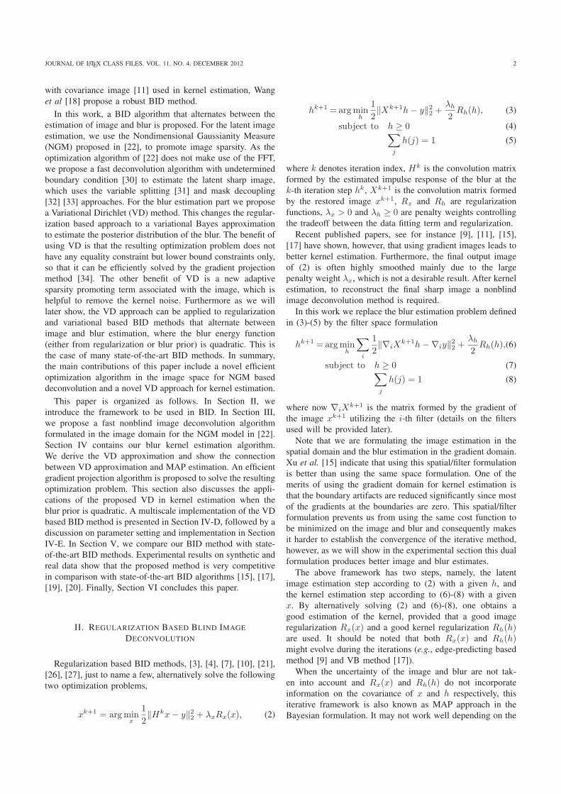
TABLE IIMAGE SPACE VS. FILTER SPACE FOR KERNEL ESTIMATION

Filter space Image spaceAverage Error Ratio 1.2257 2.1916

Average SSDs 31.9840 55.8135

2 can be applied to the quadratic regularization in [17] as anexample of how our method can be applied to other quadraticregularization methods. Before comparing our method withstate-of-the-art BID algorithms [15], [17], [19] and [20], wealso conduct two additional experiments aimed at analyzingthe numerical performance of the image estimation procedureand the impact of the regularization parameter.

All results are obtained by the default parameters unlessotherwise specified. All experiments are carried out usingMatlab 7.11 with the Intel Core i5-337U CPU @ 1.8GHz.The proposed BID method takes about 20 seconds to estimatea 19× 19 blur from a 256× 256 image.

A. Image vs. filter space for kernel estimation

The kernel estimation problem can be formulated either inthe image space (3)-(5) or the filter space, (6)-(8). In thismanuscript, we are formulating the image estimation in theimage space and the kernel estimation in the filter space.To show the superiority of this formulation, we conductedexperiments on the dataset [24], which consists of 32 blurredimages, corresponding to 4 groundtruth images and 8 motionblur kernels.

Table I reports the average SSD (sum of squared differences)and average error ratio (ratio between SSD errors of thedeconvolution with the estimated kernel and the deconvolutionwith the groundtruth kernel [24]) of all 32 restorations. It isclear that using filtered images for kernel estimation providesbetter results according to these two criteria. This conclusionis in agreement with the results obtained by Xu et al. [15].

B. Kernel Estimation with Groundtruth Image

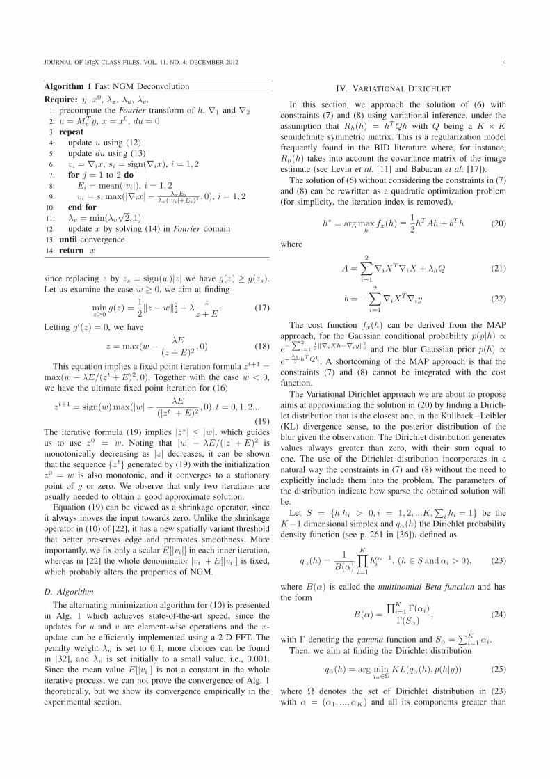
We now evaluate the performance of the backtrackinggradient projection algorithm in Alg. 2 for kernel estimation.For this purpose, we obtain the degraded image in Fig. 2(a) byblurring the cameraman image with the kernel h0 in Fig. 2(b)and corrupting the blurred image by 5% Gaussian noise. TheMATLAB function quadprog is used to solve the quadraticmodel (20) with and without the normalization constraint,where C = I . In contrast, Alg. 2 is used to find an approximatesolution to (20) with different initial points.

Table II shows the l2-norm errors between the true kerneland the ones estimated by quadprog and Alg. 2 with differentvalues for λh. The kernels obtained with λh = 1 are presentedin Fig. 2 for visual evaluation. As we can see from Table II,it is clear that quadprog with normalization constraint yieldsmore accurate solution than without normalization constraint.This occurs because the normalization constraint acts as l1regularization and therefore promotes sparsity. Consequently,the normalization constraint suppresses noise, see the notice-able noise in the background of kernel h1 in Fig. 2(c) and the

(a) Degraded2 4 6 8 10 12 14 16 18

2

4

6

8

10

12

14

16

18

(b) h0, 19× 192 4 6 8 10 12 14 16 18

2

4

6

8

10

12

14

16

18

(c) h1

2 4 6 8 10 12 14 16 18

2

4

6

8

10

12

14

16

18

(d) h2

2 4 6 8 10 12 14 16 18

2

4

6

8

10

12

14

16

18

(e) h3

2 4 6 8 10 12 14 16 18

2

4

6

8

10

12

14

16

18

(f) h4

0 5 10 15 20−0.02

0

0.02

0.04

0.06

0.08

0.1

h(i,1

2)

i

h0

h1

h2

h3

h4

(g)

21 200 500 1001−50

−40

−30

−20

−10

0

L(α)

Iterations

α0 = 1α0 = 100000

361

(h)

Fig. 2. Kernel estimation by solving model (20) with λh = 1. (a) Degradedimage. (b) Groundtruth kernel. (c) quadprog with nonnegative constraintsonly. (d) quadprog with nonnegative and normalization constraints. (e) Alg.2with α0 = 100000

361. (f) Alg.2 with α0 = 1. (g) The 12th column vectors of

the 5 kernels. (h) Evolutions of L(α) with different initial points. Plots (b)-(f)are best viewed on the screen.

TABLE IIl2-NORM ERROR OF THE KERNELS ESTIMATED BY SOLVING THE

QUADRATIC MODEL (20) WITH DIFFERENT λh AND OPTIMIZATIONMETHODS.

λh quadprog Alg. 2with (7) only with (7) and (8) α0 = 100000

361α0 = 1

0 0.0462 0.0315 0.0311 0.0304

0.01 0.0462 0.0315 0.0311 0.0304

0.1 0.0462 0.0315 0.0311 0.0303

1 0.0463 0.0314 0.0310 0.0303

5 0.0465 0.0312 0.0308 0.0301

10 0.0468 0.0310 0.0306 0.0300

50 0.0502 0.0327 0.0324 0.0321

100 0.0561 0.0397 0.0395 0.0394

little noise in kernel h2 in Fig. 2(d) for comparison. As we cansee from Fig. 2(g), kernel h1 has larger errors than the othersat many locations, especially at (5, 12), where h1 has an errorover 0.01 while the errors of the rest kernels are about 0.005.

Table II and Fig. 2 also show that Alg. 2 produces slightlybetter results than quadprog with both constraints. This isbecause the cost function L(α), derived from the VD ap-proach, has an adaptive sparsity term, which leads to a moresparse solution (see kernel h2 in Fig. 2(d) and h4 in Fig.2(f) with less noise). Fig. 2(e) looks slightly more noisy thanFig. 2(f) because the adaptive sparsity term is diminished by


(a) (b)

(c) (d)

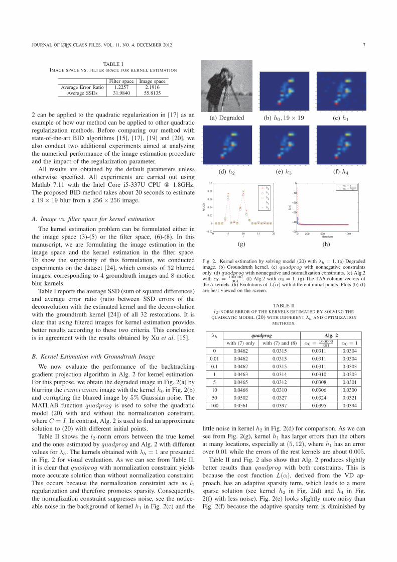
Fig. 3. Variational Dirichlet approximation vs. l1 regularization with non-negative constraints. (a) Cameraman, 256×256. (b) Degraded image withthe groundtruth kernel. (c) Restored image with the kernel estimated by [17],PSNR=24.37 dB, SSIM=0.8268. (d) Restored image with the kernel estimatedby [17] + Alg. 2, PSNR=27.61 dB, SSIM=0.8732.

large Sα. To further show that an approximate solution tomodel in (20) can be obtained by Alg. 2, we observe that||h3−h2||2 = 0.0017 and ||h4−h2||2 = 0.0052. ||h3−h2||2 is3 times smaller than ||h4−h2||2, indicating that large α0 yieldsa better approximate solution to model (20) since the adaptivesparsity term could be diminished by large Sα (see (31)). Theevolution of the cost function L(α), shown in Fig. 2(h), showsthat the proposed backtracking gradient projection algorithm isquite efficient, especially for small values of α0 (e.g., α0 = 1),since L(α) drops rapidly in less than 20 iterations.

In summary, this experiment indicates that the normalizationconstraint is important for a precise blur estimation and VDapproximation leads to a less noisy kernel than MAP.

C. Application of Alg. 2 to Babacan et al. [17]

Since matrix A in (36) is symmetric and positive definite,we can use the proposed VD to find an approximate solutionto (36). We just replace the kernel estimation in [17] with Alg.2 (default parameters) while keeping the rest unchanged, andcompare the resulting BID algorithm with [17]. We use thesynthetic image in Fig. 3(b) obtained by blurring the image inFig. 3(a) and adding a 1% Gaussian noise. To handle the noisein the images, once the kernels are obtained, we reconstructthe images using [38]. As we can see from Fig. 3(c) and (d),the proposed VD improves the result significantly, in termsof ringing artifacts, PSNR and SSIM [39]. Such a remarkableimprovement is mainly due to the normalization constraint andthe adaptive sparsity promoting term, which helps suppressthe noise in kernel (see the kernels in Fig. 3(c) and (d) for

(a) (b)

Fig. 4. The evolutions of F (x) and Rx(x), λx = 0.0002. (a) Withcontinuation. (b) Without continuation.

comparison). In addition, the method in [17] needs 122.03seconds to estimate the blur, whereas only 63.29 seconds areneeded when our Alg. 2 is incorporated into [17].

D. Numerical performance of Alg. 1

To show the convergence of Alg. 1, we use the blurredimage in Fig. 2(b) as the input image and test Alg. 1with the groundtruth kernel and 1000 iterations. The evo-lutions of F (x) = 1

2‖Hx − y‖22 + Rx(x) and Rx(x) =

λx

∑2i=1

∑Nj=1 |∇ix(j)|/(|∇ix(j)| +

∑j |∇ix(j)|/N) are

shown in Fig. 4. As we can see from Fig. 4(a), where thecontinuation scheme λv = min(

√2λv, 1) is applied, the values

of both the objective function and regularization term dropquickly and converge rapidly, but with a small jump when λv

reaches 1. In contrast, as shown in Fig. 4(b) where λv is fixedto 1, the two functions decrease slower but more smoothly.

E. The Impact of λx on Kernel Estimation

λx is the most important parameter in the proposed BIDmethod. Increasing λx makes images smoother. As a result,less gradient information is used in kernel estimation. Toutilize as much gradient information as possible, we shoulduse a small λx. However, we do not want the noise to alterthe kernel estimation. Hence, a tradeoff between removingnoise and preserving edge information should be made. Ingeneral, if the noise standard deviation increases, λx shouldalso be increased. Fig. 5 shows the impact of λx on kernelestimation, where the groundtruth and observation images areshown in Figs. 3 (a) and (b), respectively. Figs. 5(c) and5(d) show the corresponding estimation of x obtained by theproposed method. Figs. 5(c) and 5(d) are highly smoothed andcartoon like. Fig. 5(d) is more suitable for kernel estimationthan Fig. 5(c) because it has sufficient gradient informationand much less noise. Clearly, λx determines how much andwhich gradient information is allowed to participate in kernelestimation.

F. Blind Image Deconvolution on Synthetic Data

We start with the widely used dataset [24], which consists of32 blurred images, corresponding to 4 groundtruth images and8 motion blur kernels. We compare the proposed BID method,using NGM and identity or Laplacian operator, with the state-of-the-art BID methods Cho and Lee [9], Levin et al. [11],


(a) (b)

(c) (d)

Fig. 5. (a) Restored image by λx = 0.0002 and λh = 0.01, PSNR=24.03dB, SSIM=0.8418. (b) Restored image by λx = 0.0005 and λh = 0.01,PSNR=28.01, SSIM=0.8869. (c) The final x that produces the kernel shownin (a). (d) The final x that produces the kernel shown in (b).

Babacan et al. [17] and Sun et al. [19]. In [19], two imagepriors are proposed, i.e., natural and synthetic priors (see [19]for details). Since the overall performance with both priorsis similar, we report their results obtained by synthetic priorsonly. For fair comparison, once the kernel has been estimatedby each method, we use the nonblind deconvolution method[40] with the same parameters in [11] to reconstruct the finalsharp image. The parameters of the proposed algorithm arefixed to λx = 0.00015 and λh = 0.01 for all input images. Fig.6(a) shows that the proposed method has the best performancein terms of error ratio with 93.75% of the results under errorratio 2 and 96.88% less than 3. One deblurring example, whichis very challenging, is shown in Fig. 6(b-g). To the best of ourknowledge, most of the existing BID methods do not reach anerror ratio below 2 for this blurred image. In what follows, forsimplicity, all of the kernels are obtained by using C = I .

As the dataset [24] is nearly noise free, we also carry outa set of experiments on Sun’s dataset [19], which contains640 images synthesized by blurring 80 natural images with8 motion blur kernels borrowed from [24]. In this dataset,1% Gaussian noise is added to every blurred image. Insteadof using the whole dataset, we select 40 images synthesizedfrom the 5 natural images shown in the top row of Fig. 7.Again, we fix the parameters λx = 0.0002 and λh = 100

1 1.5 2 2.5 3 3.5 4 4.5 50

10

20

30

40

50

60

70

80

90

100

Error ratios

Succ

ess

perc

ent

Levin et alBabacan et alCho & LeeSun et alNGM+identityNGM+Laplacian

(a) (b) (c)

(d) (e) (f) (g)

Fig. 6. Quantitative and qualitative evaluation on data set [24]. (a) Cumulativehistograms of the error ratios across the data set [24]. (b) One blurred imageof the data set. (c) Groundtruth. (d) Babacan et al [17], error ratio =15.327. (e) Levin et al [11], error ratio = 2.462. (f) NGM+indentity,error ratio = 1.656. (g) NGM+Laplacian, error ratio = 1.687

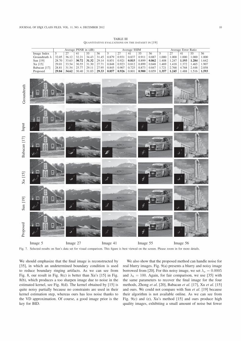
for all input images. Note that a much higher value for λh isused to deal with noise and large image size. We compare theproposed method with Babacan et al. [17], Xu et al. [15] andSun et al. [19]. Since [19] provides better results than manyexisting methods for this data set, including [9], [14], [11] and[12], we do not report the results by these methods. For faircomparison, we use the nonblind deconvolution method [38]to reconstruct the final sharp image with the PSF estimatedwith each method. We choose PSNR, SSIM [39] and errorratio [24], calculated by using the MATLAB code providedby [19], to evaluate the recovered images. Table III showsthe overall performance of the four compared methods. Theaverage error ratio in Table III shows that all methods canhandle 1% Gaussian noise very well, except [17]. The resultsobtained by the proposed method are much better than the restfor the images number 5 and 27, in terms of all measures,and similar to the results of Sun et al. [19] for the otherimages. We present the estimated images and kernels in Fig.7 for visual comparison. Our kernels are clean and visuallyaccurate, thanks to the VD approximation, except for image55 where the kernel is a bit too smooth. All the restoredimages by the proposed method are of high quality with fewerringing artifacts. For example, for image 5, our result exhibitsfewer ringing artifacts around the gate region than the others,indicating that our kernel is more accurate. For that particularimage, we report that the PSNR is 30.36 dB, just about 0.8dB less than the known kernel restoration (PSNR=31.12 dB),and the SSIM is 0.8439, just about 0.007 below the knownkernel case (SSIM=0.8506).

G. Blind Image Deconvolution on Real Data

First of all, we show that our deblurring algorithm removeslarge motion blurs. We select one severely blurred image (seeFig. 8(a)) from the dataset [41]. For this image, we set lb = 0.1and λh = 100 to deal with large blur and image, respectively.


TABLE IIIQUANTITATIVE EVALUATIONS ON THE DATASET IN [19]

Average PSNR in (dB) Average SSIM Average Error RatioImage Index 5 27 41 55 56 5 27 41 55 56 5 27 41 55 56Groundtruth h 32.05 36.12 32.21 34.43 31.45 0.879 0.931 0.837 0.911 0.887 1.000 1.000 1.000 1.000 1.000Sun [19] 28.70 33.63 30.72 31.32 29.14 0.851 0.921 0.815 0.899 0.862 1.408 1.247 1.193 1.284 1.642Xu [15] 29.01 33.54 30.55 31.30 27.71 0.848 0.923 0.812 0.899 0.848 1.469 1.418 1.372 1.465 1.907Babacan [17] 28.81 31.54 25.77 29.11 27.95 0.845 0.907 0.725 0.873 0.847 1.721 2.768 4.768 2.448 2.058Proposed 29.84 34.62 30.40 31.03 29.33 0.857 0.926 0.801 0.900 0.859 1.357 1.245 1.488 1.516 1.593

Gro

undt

ruth

Inpu

tB

abac

an[1

7]X

u[1

5]Su

n[1

9]Pr

opos

ed

Image 5 Image 27 Image 41 Image 55 Image 56Fig. 7. Selected results on Sun’s data set for visual comparison. This figure is best viewed on the screen. Please zoom in for more details.

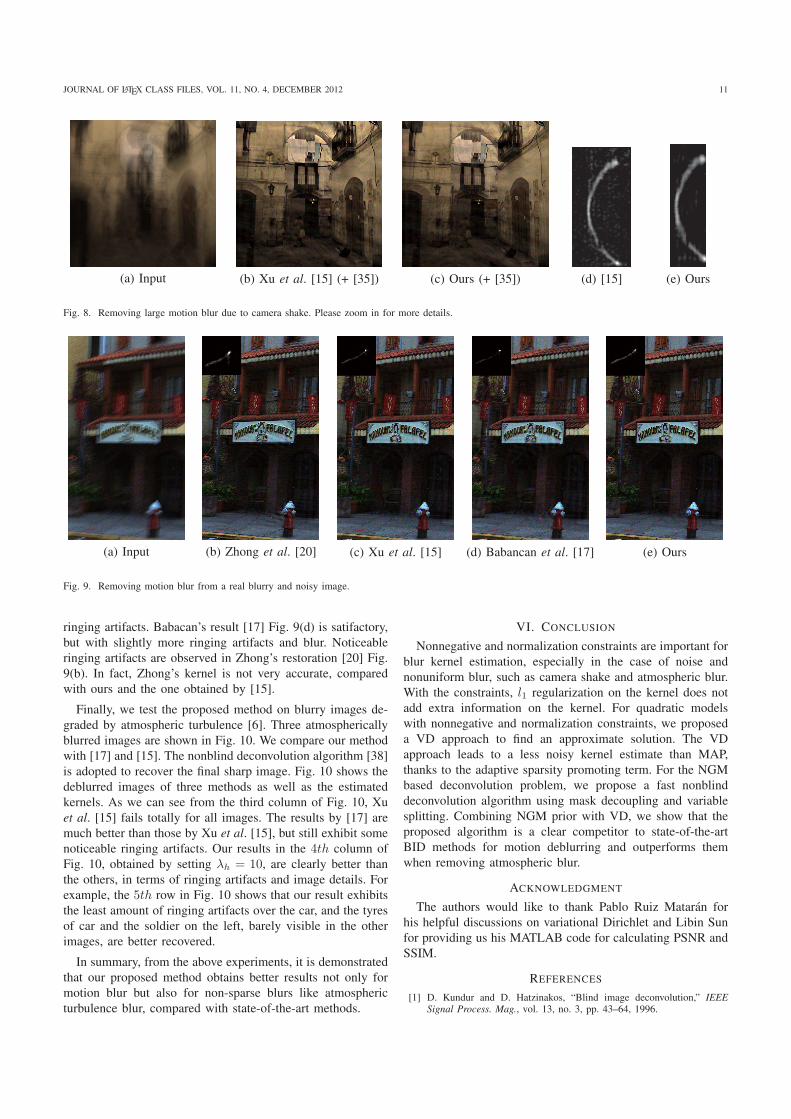
We should emphasize that the final image is reconstructed by[35], in which an undetermined boundary condition is usedto reduce boundary ringing artifacts. As we can see fromFig. 8, our result in Fig. 8(c) is better than Xu’s [15] in Fig.8(b), which produces a too sharpen image due to noise in theestimated kernel, see Fig. 8(d). The kernel obtained by [15] isquite noisy partially because no constraints are used in theirkernel estimation step, whereas ours has less noise thanks tothe VD approximation. Of course, a good image prior is thekey for BID.

We also show that the proposed method can handle noise forreal blurry images. Fig. 9(a) presents a blurry and noisy imageborrowed from [20]. For this noisy image, we set λx = 0.0005and λh = 100. Again, for fair comparison, we use [35] withthe same parameters to recover the final image for the fourmethods, Zhong et al. [20], Babacan et al. [17], Xu et al. [15]and ours. We could not compare with Sun et al. [19] becausetheir algorithm is not available online. As we can see fromFig. 9(c) and (e), Xu’s method [15] and ours produce highquality images, exhibiting a small amount of noise but fewer


(a) Input (b) Xu et al. [15] (+ [35]) (c) Ours (+ [35]) (d) [15] (e) Ours

Fig. 8. Removing large motion blur due to camera shake. Please zoom in for more details.

(a) Input (b) Zhong et al. [20] (c) Xu et al. [15] (d) Babancan et al. [17] (e) Ours

Fig. 9. Removing motion blur from a real blurry and noisy image.

ringing artifacts. Babacan’s result [17] Fig. 9(d) is satifactory,but with slightly more ringing artifacts and blur. Noticeableringing artifacts are observed in Zhong’s restoration [20] Fig.9(b). In fact, Zhong’s kernel is not very accurate, comparedwith ours and the one obtained by [15].

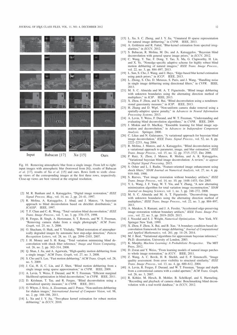
Finally, we test the proposed method on blurry images de-graded by atmospheric turbulence [6]. Three atmosphericallyblurred images are shown in Fig. 10. We compare our methodwith [17] and [15]. The nonblind deconvolution algorithm [38]is adopted to recover the final sharp image. Fig. 10 shows thedeblurred images of three methods as well as the estimatedkernels. As we can see from the third column of Fig. 10, Xuet al. [15] fails totally for all images. The results by [17] aremuch better than those by Xu et al. [15], but still exhibit somenoticeable ringing artifacts. Our results in the 4th column ofFig. 10, obtained by setting λh = 10, are clearly better thanthe others, in terms of ringing artifacts and image details. Forexample, the 5th row in Fig. 10 shows that our result exhibitsthe least amount of ringing artifacts over the car, and the tyresof car and the soldier on the left, barely visible in the otherimages, are better recovered.

In summary, from the above experiments, it is demonstratedthat our proposed method obtains better results not only formotion blur but also for non-sparse blurs like atmosphericturbulence blur, compared with state-of-the-art methods.

VI. CONCLUSION

Nonnegative and normalization constraints are important forblur kernel estimation, especially in the case of noise andnonuniform blur, such as camera shake and atmospheric blur.With the constraints, l1 regularization on the kernel does notadd extra information on the kernel. For quadratic modelswith nonnegative and normalization constraints, we proposeda VD approach to find an approximate solution. The VDapproach leads to a less noisy kernel estimate than MAP,thanks to the adaptive sparsity promoting term. For the NGMbased deconvolution problem, we propose a fast nonblinddeconvolution algorithm using mask decoupling and variablesplitting. Combining NGM prior with VD, we show that theproposed algorithm is a clear competitor to state-of-the-artBID methods for motion deblurring and outperforms themwhen removing atmospheric blur.

ACKNOWLEDGMENT

The authors would like to thank Pablo Ruiz Mataran forhis helpful discussions on variational Dirichlet and Libin Sunfor providing us his MATLAB code for calculating PSNR andSSIM.

REFERENCES

[1] D. Kundur and D. Hatzinakos, “Blind image deconvolution,” IEEESignal Process. Mag., vol. 13, no. 3, pp. 43–64, 1996.


Input Babacan [17] Xu [15] Ours

Fig. 10. Removing atmospheric blur from a single image. From left to right:input images with atmospheric blur (borrowed from [6]), results of Babacanet al. [17], results of Xu et al. [15] and ours. Rows forth to sixth: close-up views of the corresponding images at the first three rows, respectively.Close-up views are best viewed at the original resolution.

[2] M. R. Banham and A. Katsaggelos, “Digital image restoration,” IEEESignal Process. Mag., vol. 14, no. 2, pp. 24–41, 1997.

[3] R. Molina, A. Katsaggelos, J. Abad, and J. Mateos, “A bayesianapproach to blind deconvolution based on dirichlet distributions,” inICASSP. IEEE, 1997.

[4] T. F. Chan and C.-K. Wong, “Total variation blind deconvolution,” IEEETrans. Image Process., vol. 7, no. 3, pp. 370–375, 1998.

[5] R. Fergus, B. Singh, A. Hertzmann, S. T. Roweis, and W. T. Freeman,“Removing camera shake from a single photograph,” ACM Trans.Graph, vol. 25, no. 3, 2006.

[6] O. Shacham, O. Haik, and Y. Yitzhaky, “Blind restoration of atmospher-ically degraded images by automatic best step-edge detection,” PatternRecognition Letters, vol. 28, no. 15, pp. 2094–2103, 2007.

[7] J. H. Money and S. H. Kang, “Total variation minimizing blind de-convolution with shock filter reference,” Image and Vision Computing,vol. 26, no. 2, pp. 302–314, 2008.

[8] Q. Shan, J. Jia, and A. Agarwala, “High-quality motion deblurring froma single image,” ACM Trans. Graph, vol. 27, no. 3, 2008.

[9] S. Cho and S. Lee, “Fast motion deblurring,” ACM Trans. Graph, vol. 28,no. 5, 2009.

[10] J. Cai, H. Ji, C. Liu, and Z. Shen, “Blind motion deblurring from asingle image using sparse approximation,” in CVPR. IEEE, 2009.

[11] A. Levin, Y. Weiss, F. Durand, and W. T. Freeman, “Efficient marginallikelihood optimization in blind deconvolution,” in CVPR. IEEE, 2011.

[12] D. Krishnan, T. Tay, and R. Fergus, “Blind deconvolution using anormalized sparsity measure,” in CVPR. IEEE, 2011.

[13] O. Whyte, J. Sivic, A. Zisserman, and J. Ponce, “Non-uniform deblurringfor shaken images,” International Journal of Computer Vision, vol. 98,no. 2, pp. 168–186, 2011.

[14] L. Xu and J. Y. Jia, “Two-phase kernel estimation for robust motiondeblurring,” in ECCV, 2010.

[15] L. Xu, S. C. Zheng, and J. Y. Jia, “Unnatural l0 sparse representationfor natural image deblurring,” in CVPR. IEEE, 2013.

[16] A. Goldstein and R. Fattal, “Blur-kernel estimation from spectral irreg-ularities,” in ECCV, 2012.

[17] S. Babacan, R. Molina, M. Do, and A. Katsaggelos, “Bayesian blinddeconvolution with general sparse image priors,” in ECCV, 2012.

[18] C. Wang, Y. Yue, F. Dong, Y. Tao, X. Ma, G. Clapworthy, H. Lin,and X. Ye, “Nonedge-specific adaptive scheme for highly robust blindmotion deblurring of natural imagess,” IEEE Trans. Image Process.,vol. 22, no. 3, pp. 884–897, 2013.

[19] L. Sun, S. Cho, J. Wang, and J. Hays, “Edge-based blur kernel estimationusing patch priors,” in ICCP. IEEE, 2013.

[20] L. Zhong, S. Cho, D. Metaxas, S. Paris, and J. Wang, “Handling noisein single image deblurring using directional filters,” in CVPR. IEEE,2013.

[21] M. S. C. Almeida and M. A. T. Figueiredo, “Blind image deblurringwith unknown boundaries using the alternating direction method ofmultipliers,” in ICIP. IEEE, 2013.

[22] X. Zhou, F. Zhou, and X. Bai, “Blind deconvolution using a nondimen-sional gaussianity measure,” in ICIP. IEEE, 2013.

[23] H. Zhang and D. Wipf, “Non-uniform camera shake removal using aspatially-adaptive sparse penalty,” in Advances in Neural InformationProcessing Systems, 2013.

[24] A. Levin, Y. Weiss, F. Durand, and W. T. Freeman, “Understanding andevaluating blind deconvolution algorithms,” in CVPR. IEEE, 2009.

[25] J. Miskin and D. MacKay, “Ensemble learning for blind image sep-aration and deconvolution,” in Advances in Independent ComponentAnalysis. Springer, 2000.

[26] C. Likas and N. Galatsanos, “A variational approach for bayesian blindimage deconvolution,” IEEE Trans. Signal Process., vol. 52, no. 8, pp.2222–2233, Aug 2004.

[27] R. Molina, J. Mateos, and A. Katsaggelos, “Blind deconvolution usinga variational approach to parameter, image, and blur estimation,” IEEETrans. Image Process., vol. 15, no. 12, pp. 3715–3727, Dec 2006.

[28] P. Ruiz, X. Zhou, J. Mateos, R. Molina, and A. K. Katsaggelos,“Variational bayesian blind image deconvolution: A review,” to appearin Digital Signal Processing, 2015.

[29] S. Osher and L. I. Rudin, “Feature-oriented image enhancement usingshock filters,” SIAM Journal on Numerical Analysis, vol. 27, no. 4, pp.919–940, 1990.

[30] S. Reeves, “Fast image restoration without boundary artifacts,” IEEETrans. Image Process., vol. 14, no. 10, pp. 1448–1453, Oct 2005.

[31] Y. L. Wang, J. F. Yang, W. T. Yin, and Y. Zhang, “A new alternatingminimization algorithm for total variation image reconstruction,” SIAMJournal on Imaging Sciences, vol. 1, no. 3, pp. 248–272, 2008.

[32] M. S. C. Almeida and M. A. T. Figueiredo, “Deconvolving imageswith unknown boundaries using the alternating direction method ofmultipliers,” IEEE Trans. Image Process., vol. 22, no. 3, pp. 884–897,2013.

[33] A. Matakos, S. Ramani, and J. A. Fessler, “Accelerated edge-preservingimage restoration without boundary artifacts,” IEEE Trans. Image Pro-cess., vol. 22, no. 5, pp. 2019–2029, 2013.

[34] J. Nocedal and S. J. Wright, Numerical Optimization. New York, NY:Springer New York, 1999.

[35] X. Zhou, F. Zhou, X. Bai, and B. Xue, “A boundary condition based de-convolution framework for image deblurring,” Journal of Computationaland Applied Mathematics, vol. 261, pp. 14–29, 2014.

[36] M. J. Beal, “Variational algorithms for approximate bayesian inference,”Ph.D. dissertation, University of London, 2003.

[37] K. Murphy, Machine Learning: A Probabilistic Perspective. The MITPress, 2012.

[38] D. Zoran and Y. Weiss, “From learning models of natural image patchesto whole image restoration,” in ICCV. IEEE, 2011.

[39] Z. Wang, A. C. Bovik, H. R. Sheikh, and E. P. Simoncelli, “Imagequality assessment: from error visibility to structural similarity,” IEEETrans. Image Process., vol. 13, no. 4, pp. 600–612, 2004.

[40] A. Levin, R. Fergus, F. Durand, and W. T. Freeman, “Image and depthfrom a conventional camera with a coded aperture,” ACM Trans. Graph,vol. 26, no. 3, 2007.

[41] R. Kohler, M. Hirsch, B. Mohler, B. Scholkopf, and S. Harmeling,“Recording and playback of camera shake: Benchmarking blind decon-volution with a real-world database,” in ECCV, 2012.


Xu Zhou received the B.S. degree in applied mathe-matics from the Central South University, Changsha,China, in 2009. He is currently pursuing the Ph.D.degree from the Image Processing Center, BeihangUniversity, Beijing, China.

From October 2013 to October 2014, sponsoredby the Chinese Scholarship Council, he was a Vis-iting Student with the Department of ComputerScience and Artificial Intelligence, University ofGranada, Spain. His research interests include imagerestoration, machine learning, and optimization.

Javier Mateos received the degree in computerscience in 1991 and the Ph.D. degree in com-puter science in 1998, both from the Universityof Granada. He was an Assistant Professor withthe Department of Computer Science and ArtificialIntelligence, University of Granada, from 1992 to2001, and then he became a permanent AssociateProfessor. He is coauthor of Superresolution of Im-ages and Video (Claypool, 2006) and MultispectralImage fusion Using Multiscale and Super-resolutionMethods (VDM Verlag, 2011). He received the IEEE

International Conference on Signal Processing Algorithms, Architectures,Arrangements, and Applications best paper award (2013) and was finalist forthe IEEE International Conference on Image Processing Best Student PaperAward (2010). He is conducting research on image and video processing,including image restoration, image and video recovery, super-resolution from(compressed) stills and video sequences, pansharpening and image classifica-tion.

Dr. Mateos is a member of the IEEE, Asociacion Espanola de Re-conocimento de Formas y Analisis de Imagenes (AERFAI) and InternationalAssociation for Pattern Recognition (IAPR). He is editor of “Digital SignalProcessing” and serves the IEEE as an Associate Editor for the “IEEETransactions on Image Processing”.

Fugen Zhou received the B.S. degree in electronicengineering, M.S. degree and Ph.D. degree in patternrecognition and intelligent system from BeihangUniversity (formerly, Beijing University of Aeronau-tics and Astronautics), Beijing, China, in 1986, 1989,and 2006, respectively.

He joined the Image Processing Center at BeihangUniversity in 1989. Since 2007, he has been a Pro-fessor with the School of Space, Beihang University.In 2004, as a Visiting Scholar, he cooperated withthe research Institute of William Beaumont Hospital,

USA. Since 2000, He has been the Director of Image Processing Center atBeihang University. He currently serves as Associate Director of MedicalImaging Committee, Chinese Society of Medical Physics and a StandingMember of Chinese Society for Optical Engineering. One of his Ph.D.students, under his supervision, has been awarded the best doctoral thesisof BUAA in 2010 and the nomination prize of the national best doctoralthesis of China in 2011. His research interests include target detection andrecognition, multi-modality image processing, biomedical image processing& recognition. He has authored or coauthored over 70 research papers.

Rafael Molina (M88) was born in 1957. He receivedthe degree in mathematics (statistics) in 1979 andthe Ph.D. degree in optimal design in linear modelsin 1983. He became Professor of Computer Sci-ence and Artificial Intelligence at the University ofGranada, Granada, Spain, in 2000. Former Dean ofthe Computer Engineering School at the Universityof Granada (1992-2002) and Head of the ComputerScience and Artificial Intelligence department of theUniversity of Granada (2005-2007). His researchinterest focuses mainly in using Bayesian modeling

and inference in problems like image restoration (applications to astronomyand medicine), super resolution of images and video, blind deconvolution,computational photography, source recovery in medicine, compressive sens-ing, low rank matrix decomposition, active learning, fusion and classification.See http://decsai.ugr.es/∼rms for publications, funded projects and grants.

Dr. Molina serves the IEEE and other Professional Societies: Applied SignalProcessing, Associate Editor (2005-2007), IEEE Trans. on Image Processing,Associate Editor (2010–), Progress in Artificial Intelligence, Associate Editor(2011–) and Digital Signal Processing, Area Editor (2011–). He is therecipient of an IEEE International Conference on Image Processing PaperAward (2007), an ISPA Best Paper Award (2009) and coauthor of a paperawarded the runner-up prize at Reception for early-stage researchers at theHouse of Commons.

Aggelos K. Katsaggelos received the Diploma de-gree in electrical and mechanical engineering fromthe Aristotelian University of Thessaloniki, Greece,in 1979, and the M.S. and Ph.D. degrees in ElectricalEngineering from the Georgia Institute of Technol-ogy, in 1981 and 1985, respectively.

In 1985, he joined the Department of ElectricalEngineering and Computer Science at NorthwesternUniversity, where he is currently a Professor holderof the AT&T chair. He was previously the holderof the Ameritech Chair of Information Technology

(1997-2003). He is also the Director of the Motorola Center for SeamlessCommunications, a member of the Academic Staff, NorthShore UniversityHealth System, an affiliated faculty at the Department of Linguistics and hehas an appointment with the Argonne National Laboratory.

He has published extensively in the areas of multimedia signal processingand communications (over 230 journal papers, 500 conference papers and40 book chapters) and he is the holder of 25 international patents. He isthe co-author of Rate-Distortion Based Video Compression (Kluwer, 1997),Super-Resolution for Images and Video (Claypool, 2007), Joint Source-Channel Video Transmission (Claypool, 2007), and Machine Learning Refined(Cambridge University Press, forthcoming). He has supervised 50 Ph.D. thesesso far.

Among his many professional activities Prof. Katsaggelos was Editor-in-Chief of the IEEE Signal Processing Magazine (1997-2002), a BOGMember of the IEEE Signal Processing Society (1999-2001), a member of thePublication Board of the IEEE Proceedings (2003-2007), and he is currentlya Member of the Award Board of the IEEE Signal Processing Society. Heis a Fellow of the IEEE (1998) and SPIE (2009) and the recipient of theIEEE Third Millennium Medal (2000), the IEEE Signal Processing SocietyMeritorious Service Award (2001), the IEEE Signal Processing SocietyTechnical Achievement Award (2010), an IEEE Signal Processing SocietyBest Paper Award (2001), an IEEE ICME Paper Award (2006), an IEEE ICIPPaper Award (2007), an ISPA Paper Award (2009), and a EUSIPCO paperaward (2013). He was a Distinguished Lecturer of the IEEE Signal ProcessingSociety (2007-2008).

Variation Dirichlet Blur Kernel Estimation doubledecsai.ugr.es/vip/files/journals/Variation...

Documents

Transcript of Variation Dirichlet Blur Kernel Estimation doubledecsai.ugr.es/vip/files/journals/Variation...