The Effect of Jumps and Discrete Sampling on

Volatility and Variance Swaps∗

Mark Broadie# Ashish Jain†

This is the working paper version of: Broadie, M., and A. Jain, 2008, “The Effect of Jumps

and Discrete Sampling on Volatility and Variance Swaps,” International Journal of Theoretical

and Applied Finance, Vol.11, No.8. 761-797. This version fixes several typographical errors in

Table 1 in addition to other minor changes.

Abstract

We investigate the effect of discrete sampling and asset price jumps on fair variance and volatility

swap strikes. Fair discrete volatility strikes and fair discrete variance strikes are derived in differ-

ent models of the underlying evolution of the asset price: the Black-Scholes model, the Heston

stochastic volatility model, the Merton jump-diffusion model and the Bates and Scott stochastic

volatility and jump model. We determine fair discrete and continuous variance strikes analyti-

cally and fair discrete and continuous volatility strikes using simulation and variance reduction

techniques and numerical integration techniques in all models. Numerical results show that the

well-known convexity correction formula may not provide a good approximation of fair volatility

strikes in models with jumps in the underlying asset. For realistic contract specifications and

model parameters, we find that the effect of discrete sampling is typically small while the effect

of jumps can be significant.

#Columbia University, Graduate School of Business, 3022 Broadway, New York, NY, 10027-6902.

email: mnb2@columbia.edu.†Columbia University, Graduate School of Business, 3022 Broadway, New York, NY, 10027-6902.

email: aj2109@columbia.edu.

∗This paper was presented at the Fall 2006 INFORMS annual conference, the London Business School, the

2005 Winter Simulation Conference and at the Columbia Business School. We thank Peter Carr for helpful

comments. This work was partly supported by NSF grant DMS-0410234.

1

1 Introduction

Volatility and variance swaps are forward contracts in which one counterparty agrees to pay the

other a notional amount times the difference between a fixed level and a realized level of variance

and volatility, respectively. The fixed level is called the variance strike for variance swaps and

the volatility strike for volatility swaps. This is typically set initially so that the net present

value of the payoff is zero. Realized variance, or the floating leg of the swap, is determined by

the average variance of the asset over the life of the swap.

The variance swap payoff is defined as

(Vd(0, n, T ) − Kvar(n)) × N

where Vd(0, n, T ) is the realized stock variance (as defined below) over the life of the contract,

[0, T ], n is the number of sampling dates, Kvar(n) is the variance strike, and N is the notional

amount of the swap in dollars. The holder of a variance swap at expiration receives N dollars for

every unit by which the stock’s realized variance Vd(0, n, T ) exceeds the variance strike Kvar(n).

The variance strike is quoted as volatility squared, e.g., (20%)2.

The volatility swap payoff is defined as

(√

Vd(0, n, T ) − Kvol(n)) × N

where√

Vd(0, n, T ) is the realized stock volatility (quoted in annual terms as defined below) over

the life of the contract, n is the number of sampling dates, Kvol(n) is the volatility strike, and N

is the notional amount of the swap in dollars. The volatility strike Kvol(n) is typically quoted as

volatility, e.g., 20%. The procedure for calculating realized volatility and variance is specified in

the contract and includes details about the source and observation frequency of the price of the

underlying asset, the annualization factor to be used in moving to an annualized volatility and

the method of calculating the variance.

Let 0 = t0 < t1 < ... < tn = T be a partition of the time interval [0, T ] into n equal segments

of length �t, i.e., ti = iT/n for each i = 0, 1, ..., n. Most traded contracts define the realized

variance to be

Vd(0, n, T ) =AF

m

n−1∑i=0

(ln

(Si+1

Si

))2

(1)

1

for a swap covering n return observations. Typically contracts m is set to n − 1, though n is

sometimes used. Here Si is the price of the asset at the ith observation time ti and AF is the

annualization factor, e.g., 252 (= n/T ) if the maturity of the swap, T , is one year with daily

sampling. This definition of realized variance differs from the usual sample variance because the

sample average is not subtracted from each observation. Since the sample average is approxi-

mately zero, the realized variance is close to the sample variance.

Demeterfi, Derman, Kamal and Zou (1999) examined properties of variance and volatility swaps.

They derived an analytical formula for the variance strike in the presence of a volatility skew.

Brockhaus and Long (2000) provided an analytical approximation for the pricing of volatility

swaps. Javaheri, Wilmott and Haug (2002) discussed the valuation of volatility swaps in the

GARCH(1,1) stochastic volatility model. They used a partial differential equation approach to

determine the first two moments of the realized variance and then used a convexity approxima-

tion formula to price the volatility swaps. Little and Pant (2001) developed a finite difference

method for the valuation of variance swaps in the case of discrete sampling in an extended Black-

Scholes framework. Detemple and Osakwe (2000) priced European and American options on spot

volatility when volatility follows a diffusion process. Carr, Geman, Madan and Yor (2005) priced

options on realized variance by directly modeling the quadratic variation of the underlying asset

using a Levy process. Carr and Lee (2005) priced arbitrary payoffs of realized variance under a

zero correlation assumption between the stock price process and variance process. Lipton (2000)

priced volatility swaps using a partial differential equation approach. Sepp (2008) priced options

on realized variance in the Heston stochastic volatility model by solving a partial differential

equation. Buehler (2006) proposed a general approach to model a term structure of variance

swaps in an HJM-type framework. Meddahi (2002) presented quantitative measures of the real-

ized volatility in the eigenfunction stochastic volatility model for different sampling sizes.

The analysis in most of these papers is based on an idealized contract where realized variance and

volatility are defined with continuous sampling, e.g., a continuously sampled realized variance,

Vc(0, T ), defined by:

Vc(0, T ) ≡ limn→∞

Vd(0, n, T ) (2)

In this paper we analyze the differences between actual contracts based on discrete sampling and

idealized contracts based on continuous sampling. Another objective of this paper is to analyze

the effect of ignoring jumps in the underlying on fair variance swap strikes.

2

Financial models typically specify the dynamics of the stock price and variance using stochastic

differential equations (SDE) and discrete and continuous realized variance depend on the mod-

eling assumptions. The Black-Scholes model proposed in the early 1970s assumes that a stock

price follows geometric Brownian motion with a constant volatility term. This constant volatility

assumption is not typically satisfied by options trading in the market and subsequently many

different models have been proposed. Merton (1973) extended the constant volatility assumption

in Black-Scholes model to a term structure of volatility, i.e., σ = σ(t). Derman and Kani (1994)

and Derman, Kani and Zou (1996) extended this to local volatility models where volatility is

a function of two parameters, time and the current level of the underlying, i.e., σ = σ(t, S(t)).

Several models have been developed where volatility is modeled as a stochastic process often

including mean reversion. Hull and White (1987) proposed a lognormal model for the variance

process with independence between the driving Brownian motions of the stock price and variance

processes. Heston (1993) proposed a mean reverting model for variance that allows for correla-

tion between volatility and the asset level. Stein and Stein (1991) and Schobel and Zhu (1999)

proposed a stochastic volatility model in which volatility of underlying asset follows Ornstein-

Uhlenbeck process. Bates (1996) and Scott (1997) proposed a stochastic volatility with jumps

model by adding log-normal jumps in stock price process in the Heston stochastic volatility model.

Continuous realized variance depends on the model assumed for the underlying asset price.

Depending on the model, discrete realized variance and continuous realized variance can be

different. The fair strike of a variance swap (with discrete or continuous sampling) is defined to

be the strike which makes the net present value of the swap equal to zero. We call it the fair

variance strike. The fair discrete volatility strike and fair discrete variance strikes are defined

similarly. In this paper we analyze discrete variance swaps and continuous variance swaps and the

effect of the number of sampling dates on fair variance strikes and fair volatility strikes. Various

authors have proposed to replicate a variance swap using a static portfolio of out-of-the-money

call and put options. This ignores the effect of jumps in the underlying. The fair variance swap

strike will differ from the static replicating portfolio of options if the underlying has jumps. In

this paper we investigate the following questions:

• What is the effect of ignoring jumps in the underlying on fair variance swap strikes?

• What is the relationship between fair variance strikes and fair volatility strikes?

• How do fair variance strikes and fair volatility strikes vary in different models?

3

• What is the convergence rate of expected discrete realized variance to expected continuous

realized variance with the number of sampling dates? Are fair discrete variance strikes and

fair discrete volatility strikes with daily, weekly or monthly sampling significantly different

than fair continuous variance strikes and fair continuous volatility strikes, respectively?

• How well does the convexity correction formula approximate fair volatility strikes?

In this paper, we analyze all these issues under four different models of underlying evolution

of asset price: the Black Scholes model (BS), the Heston stochastic volatility model (SV), the

Merton jump-diffusion model (J) and stochastic volatility with jumps model (SVJ).

The rest of the paper is organized as follows. We begin briefly by introducing volatility derivatives

in section 2 and provide formulas to price these derivatives. Convergence rates of discrete variance

strikes to continuous variance strikes in the Black-Scholes model are derived. In sections 3, 4

and 5, we present analysis for the models J, SV, and SVJ, respectively. In section 6 we present

numerical results and concluding remarks are given in section 7.

2 Volatility derivatives

2.1 Variance swaps

In this section, we provide definitions of discretely sampled realized variance and continuously

sampled realized variance and review how to replicate variance swaps when the stock price process

is continuous. We assume the risk neutral dynamics of the underlying asset St are given by:

dSt

St= rdt + σtdW Q

t (3)

where r is the risk free rate, W is a standard Brownian motion under the risk-neutral measure

Q. We assume throughout in this paper that there exists a unique risk-neutral measure Q. The

parameter σt represents the level of volatility. The standard Black-Scholes model assumes that

this parameter is constant, while in stochastic volatility models σt is specified by another diffu-

sion process, as in the Heston stochastic volatility model (SV) in section 4.

A variance swap is a forward contract on the realized variance of underlying security. The floating

leg of variance swap is the realized variance and is calculated using the second moment of log

4

returns of the underlying asset:

Ri = ln

(Sti

Sti−1

), i = 1, 2, ..., n

where 0 = t0 < t1 < ... < tn = T is a partition of the time interval [0, T ] into n equal segments

of length �t, i.e., ti = iT/n for each i = 0, 1, ..., n. The discrete realized variance, Vd(0, n, T ),

from equation (1) can be written as:

Vd(0, n, T ) =1

(n − 1)Δt

n∑i=1

R2i =

∑n−1i=0 (ln(Si+1

Si))2

(n − 1)Δt(4)

The floating leg of the variance swap, or the discretely sampled realized variance, in the limit

approaches the continuously sampled realized variance, Vc(0, T ), that is:

Vc(0, T ) ≡ limn→∞

Vd(0, n, T ) = limn→∞

n

(n − 1)T

n∑i=1

R2i (5)

Jacod and Protter (1998) provide necessary and sufficient conditions for the rate of convergence of

the Euler scheme approximation of the solution to a stochastic differential equation to be 1/√

n.

The discrete realized variance, Vd(0, n, T ), is the Euler scheme approximation of the stochastic

differential equation (3) followed by underlying asset St when sampling size is n. Thus, the rate

of convergence of discrete realized variance, Vd(0, n, T ), to continuous realized variance, Vc(0, T ),

is 1/√

n.

In the case of the Black-Scholes model and the Heston stochastic volatility model, continuous

realized variance is given by:1

Vc(0, T ) =1

T

∫ T

0

σ2t dt (6)

Continuous realized variance can be replicated by a static position in a log contract (Demeterfi

et al. 1999) and a dynamic trading strategy in the underlying asset. Applying Ito’s lemma to

equation (3) we get

ln

(ST

S0

)=

∫ T

0

(r − 1

2σ2

t

)dt +

∫ T

0

σtdW Qt (7)

Subtracting equation (7) from equation (3) and rearranging we get

2

T

( ∫ T

0

dSt

St− ln

ST

S0

)=

1

T

∫ T

0

σ2t dt = Vc(0, T ) (8)

1Equation (6) holds for asset price models following the dynamics in (3). When jumps are introduced the

definition of Vc(0, T ) will be different.

5

Equation (8) shows that continuous realized variance can be replicated by a short position in

the log contract and payoffs from a dynamic trading strategy which holds 1/St shares of the

underlying stock at each instant of time t. In particular, equation (8) holds in the Black-Scholes

model and the Heston stochastic volatility model.

Next, we give definitions of realized variance and accumulated variance with discrete sampling

and continuous sampling. Continuous realized variance between time t and T is given by

Vc(t, T ) =1

T

∫ T

t

σ2sds (9)

Continuous accumulated variance from the start of the contract (time 0) until time t is defined

by

Ic(t, T ) =1

T

∫ t

0

σ2sds (10)

From equations (9) and (10) we can write

Vc(0, T ) = Ic(t, T ) + Vc(t, T )

We define Pc(t, T, K, Ic) to be the expected present value at time t of the payoff of a continuous

variance swap with variance strike, K, i.e.,

Pc(t, T, K, Ic) = EQt

(e−r(T−t)

(Ic + Vc(t, T ) − K

))(11)

where the superscript Q denotes the risk-neutral measure and the subscript t denotes expectation

at time t and Ic = Ic(t, T ) . Throughout this paper expectation is always in the risk-neutral

measure so we will drop the superscript. The fair continuous variance strike, K∗var, is defined to

be the strike such that the net present value of the swap at time t = 0 is zero, i.e.,

Pc(0, T, K∗var, Ic) = E0

(e−rT

(Vc(0, T ) − K∗

var

))= 0 (12)

where Ic = Ic(0, T ) = 0. Solving (12) for K∗var gives

K∗var = E0[Vc(0, T )] = E0

[1

T

∫ T

0

σ2sds

](13)

The discrete realized variance between times ti = iT/n and T when there are n sampling dates

between the start of contract at t = 0 and its maturity at t = T is given by

Vd(i, n, T ) =

∑n−1j=i (ln(

Sj+1

Sj))2

(n − 1)Δt(14)

6

The discrete accumulated variance from the start of the contract, t = 0, until time ti is

Id(i, n, T ) =

∑i−1j=0(ln(

Sj+1

Sj))2

(n − 1)Δt(15)

From equations (14) and (15) we can write

Vd(0, n, T ) = Id(i, n, T ) + Vd(i, n, T )

We define Pd(i, n, T, K, Id(i, n, T )) to be the expected present value at time ti = iT/n of the

payoff of a discrete variance swap with strike K and it is given by

Pd(i, n, T, K, Id) = Eti

(e−r(T−ti)

(Id + Vd(i, n, T ) − K

))(16)

where Id = Id(i, n, T ). The fair discrete variance strike, K∗var(n), is defined to be the strike such

that the expected net present value of the swap at time t = 0 is zero. i.e.,

Pd(0, n, T, K∗var(n), Id) = E0

(e−rT

(Vd(0, n, T ) − K∗

var(n)

))= 0 (17)

where Id = Id(0, n, T ) = 0.At time t = 0, Pd(0, n, T, K, Id) can be written as

Pd(0, n, T, K, Id) = Pc(0, T, K, Ic) + E0

(e−rT

(Vd(0, n, T ) − Vc(0, T )

))= Pc(0, T, K, Ic) + e−rT

(K∗

var(n) − K∗var

)(18)

In above equation both Id and Ic equals zero. We will use these definitions to show the linear

convergence rate of Pd(0, n, T, K, Id) to Pc(0, T, K, Ic).

2.2 Volatility swaps

The floating leg of a volatility swap on an asset S is the realized volatility of that asset’s price.

This volatility is commonly calculated using the square root of the realized variance defined in

equation (4). The fair strike K∗vol of a continuous volatility swap is set at the initiation of the

contract so that the contract’s net present value is equal to zero, i.e.,

E0

[e−rT (

√Vc(0, T ) − K∗

vol)

]= 0 (19)

Solving (19) for the fair continuous volatility strike, K∗vol, we get

K∗vol = E[

√Vc(0, T )] = E0

[√1

T

∫ T

0

σ2sds

]Similarly, the fair discrete volatility strike is given by:

K∗vol(n) = E0

[√Vd(0, n, T )

](20)

7

2.3 Convexity correction formula

In this section we present the convexity correction formula (Brockhaus and Long 2000) to ap-

proximate fair volatility strikes. Then we present an argument to show why in some cases it may

not provide an accurate approximation.

Jensen’s inequality shows that the fair volatility strike is bounded above by the square root of

the fair variance strike:2

K∗vol = E0[

√Vc(0, T )] ≤

√E0[Vc(0, T )] =

√K∗

var (21)

A similar result holds in the discrete case:

K∗vol(n) = E0[

√Vd(0, n, T )] ≤

√E0[Vd(0, n, T )] =

√K∗

var(n) (22)

Brockhaus and Long (2000) provide a convexity correction formula for calculating the fair volatil-

ity strike using a Taylor’s expansion of the square root function. A second order Taylor’s expan-

sion of f(x) =√

x around x0 gives

√x =

√x0 +

(x − x0)

2√

x0− (x − x0)

2

8x032

+ f (3)(ε)(x − x0)

3

3!(23)

where f (3) is the 3rd derivative of function f(x) for some ε in (x0, x). The first three terms on

the right hand side provide a good approximation of√

x for all values of x in the neighborhood

of x0 for which Taylor’s series converges. For Taylor’s series to converge, x− x0 should lie in the

radius of convergence, which for the square root function is

|x − x0| ≤ x0 (24)

When this condition holds, the last term in equation (23) is bounded and the first three terms

provide a good estimate to compute the value of function at a point, in this case√

x. Now,

substitute x = Vc(0, T ) and x0 = E[Vc(0, T )] in equation (23) to get:

√Vc(0, T ) ≈

√E[Vc(0, T )] +

(Vc(0, T ) − E[Vc(0, T )])

2√

E[Vc(0, T )]− (Vc(0, T ) − E[Vc(0, T )])2

8E[Vc(0, T )]32

(25)

2For the concave square root function Jensen’s inequality is:

E(√

x) ≤√

E(x)

8

The terms on the right hand side in equation (25) provide a good estimate of the square root

of the realized variance√

Vc(0, T ) on a single stock price path if the realized variance Vc(0, T )

satisfies the condition:

|Vc(0, T ) − E(Vc(0, T ))| ≤ E(Vc(0, T )) (26)

which can also be rewritten as

0 ≤ Vc(0, T ) ≤ 2E(Vc(0, T )) (27)

If condition (27) holds on all stock price paths under the risk-neutral measure then the right

hand side of equation (25) provides a good estimate of square root of realized variance√

Vc(0, T )

on all stock price paths. Taking expectations under the risk-neutral measure on both sides of

(25) gives:

K∗vol ≈

√K∗

var −Var(Vc(0, T ))

8E[Vc(0, T )]32

(28)

The convexity correction formula (28) can be used to approximate fair volatility strikes. The

2nd order term in (28) is the convexity correction term. This approximation should work well if

condition (27) holds on all sample paths. Noting that the excess probability

p ≡ P (Vc(0, T ) ≥ 2E(Vc(0, T ))), (29)

condition (27) is equivalent to the excess probability, p, being equal to zero. A discrete version

of (28) can be used to approximate fair discrete volatility strikes and this approximation should

work well if (27) is satisfied by the discrete realized variance.

When the excess probability (29) is not equal to zero then the higher order terms in the Taylor’s

expansion are not negligible compared to the first three terms in the expansion. If we include

the 3rd and 4th order expansion terms in (28) we get

E[√

Vc(0, T )] ≈√

E[Vc(0, T )] +(Vc(0, T ) − E[Vc(0, T )])

2√

E[Vc(0, T )]− (Vc(0, T ) − E[Vc(0, T )])2

8E[Vc(0, T )]32

+(Vc(0, T ) − E[Vc(0, T )])3

16E[Vc(0, T )]52

− 5(Vc(0, T ) − E[Vc(0, T )])4

128E[Vc(0, T )]72

(30)

When p is not equal to zero then the higher moments of Vc(0, T )−E(Vc(0, T )) are not negligible.

9

In the Black-Scholes model, the excess probability is equal to zero in the continuous case and

the higher moments of continuous realized variance are zero since volatility is constant. Hence,

the convexity correction formula holds with equality in (28) in the Black-Scholes model and can

be used to compute the fair continuous volatility strike.

In the discrete case, i.e., for a finite number of sampling dates n, the excess probability is not

equal to zero and the higher moments of the discrete realized variance in the Black-Scholes model

are not zero. The magnitude of the 3rd and 4th order terms are comparable to first two terms and

the excess probability p is not zero with discrete sampling in the Black-Scholes model. Hence,

the convexity correction formula (28) will not provide a good approximation of the fair volatility

strike in the Black-Scholes model when the number of sampling dates n is small.

In the Heston stochastic volatility model, the excess probability p is not equal to zero, the 3rd

and 4th order terms in equation (30) are not small and hence the convexity correction approxi-

mation will not provide a good estimate of the fair volatility strike. This is true in the Merton

jump-diffusion model as well. Section 6 provides numerical results illustrating the computation

of volatility strikes from the convexity correction formula, the 3rd and 4th order terms in equation

(30) and the excess probability in all three models.

3 Merton jump-diffusion model

In this section, we present an analysis of the convergence of discrete variance strikes to continuous

variance strikes with number of sampling dates in the Merton jump-diffusion (J) model. The

risk-neutral dynamics of the jump-diffusion model are given by:

dSt

S−t

= (r − λm)dt + σdW Qt + dJt (31)

where Jt =∑Nt

i=1(Yj − 1) and Nt is a Poisson process with rate λ and Yj is the relative jump size

in the stock price. When jump occurs at time τj , then S(τ+j ) = S(τ−

j )Yj, where the distribution

of Yj is LN[a, b2] and m is the mean proportional size of jump E(Yj − 1) = m. The parameters a

and m are related to each other by the equation: ea+ 12b2 = m+1 and only one of them needs to be

specified. Results for the Black-Scholes model are given by setting the jump parameter, λ, to zero.

10

In the case of continuous sampling, realized variance consists of two components. The first is

the accumulated variance contributed from the diffusive component of the underlying asset price

process and second is the contribution from jumps. If there are N(T ) price jumps in [0, T ], the

contribution to the realized variance from jumps is

1

T

( N(T )∑i=1

(ln(Yi))2

)Thus, the continuous realized variance in the Merton jump-diffusion model can be expressed as

Vc(0, T ) =1

T

∫ T

0

σ2dt +1

T

( N(T )∑i=1

(ln(Yi))2

)= σ2 +

1

T

( N(T )∑i=1

(ln(Yi))2

)(32)

The fair continuous variance strike is obtained by taking the expectation of the continuous

realized variance:

K∗var = E0[Vc(0, T )] = σ2 + λ(a2 + b2) (33)

In the jump-diffusion model, the fair continuous variance strike depends on the continuous volatil-

ity parameter σ and the volatility of the stock from the jumps during the life of contract. Depend-

ing on the relative size of the jump parameters, realized variance can be significantly different

than in other models.

3.1 Jump-Diffusion Model: Continuous Volatility Strike

In this section we derive a formula for the fair continuous volatility strike in the Merton jump-

diffusion model. The continuous realized variance in the Merton jump-diffusion model is given

by equation (32). The square root function can be expressed (Schurger 2002) as:

√x =

1

2√

π

∫ ∞

0

1 − e−sx

s32

ds (34)

Taking expectations on both sides of (34) and interchanging the expectation and integral using

Fubini’s theorem we get

E(√

x) =1

2√

π

∫ ∞

0

1 − E(e−sx)

s32

ds (35)

The fair continuous volatility strike can be evaluated using (35), numerical integration, and the

expression for expectation in the integral given in the next proposition.

11

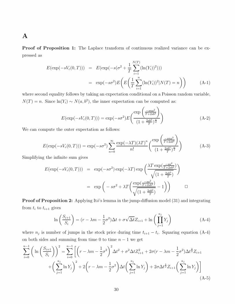
Proposition 1 In the Merton jump-diffusion model, the Laplace transform of the continuous

realized variance E(exp(−sVc(0, T ))) is given by:

E(exp(−sVc(0, T ))) = exp

(− sσ2 + λT

(exp( −sa2

T+2sb2)√

(1 + 2sb2

T)− 1

))(36)

All proofs are given in Appendix A.

3.2 Merton jump-diffusion model: discrete variance strike

Proposition 2 In the Merton jump-diffusion model

E0

(Vd(0, n, T )

)= E0

(Vc(0, T )

)+ f(r, a, b, σ, λ, m, T, n)

= σ2 + (a2 + b2)λ + f(r, a, b, σ, λ, m, T, n) (37)

where the function f(r, a, b, σ, λ, m, T, n) converges to zero linearly with number of sampling dates

n and

f(r, a, b, σ, λ, m, T, n) =σ2 + (a2 + b2)λ + (r − λm − 1

2σ2)2T + a2λ2T + 2(r − λm − 1

2σ2)aλT

n − 1

The expectation of discrete realized variance converges to the expected continuous realized variance

linearly with the sampling size (n = T/Δt). Consequently

K∗var(n) = K∗

var + f(r, a, b, σ, λ, m, T, n) (38)

and the fair discrete variance strike converges to the fair continuous variance strike linearly with

number of sampling dates (n= T/Δt).

Hence, from equation (18) the initial value of a discrete variance swap, Pd(0, n, T, K, I), converges

linearly to the initial value of a continuous variance swap, Pc(0, T, K, I), with the number of

sampling dates.

3.3 Merton jump-diffusion model: discrete volatility strike

In this section we compute the fair discrete volatility strike in the Merton jump-diffusion model.

We can compute the fair discrete volatility strike by using formula (35).

12

Proposition 3 In the Merton jump-diffusion model, the Laplace transform of the discrete real-

ized variance E(exp(−sVd(0, n, T ))) is given by:

E

(exp(−sVd(0, n, T ))

)=

( ∞∑ni=0

exp(−λΔt)(λΔt)ni

ni!

(exp

(−s((r−λm− 1

2σ2)Δt+ani)

2

(n−1)Δt+2s(σ2Δt+b2ni)

)√

(1 + 2s(σ2Δt+b2ni)(n−1)Δt

)

))n

(39)

The expectation in (39) can be computed numerically since the sum converges very fast. We

use the Laplace transform and formula (35) to compute the fair discrete volatility strike in the

Merton jump-diffusion model.

4 Heston stochastic volatility model

In this section, we present an analysis of the convergence of discrete variance strikes to continuous

variance strikes with number of sampling dates in the Heston stochastic volatility (SV) model.

The Heston (1993) model is given by:

dSt = rStdt +√

vtSt(ρdW 1t +

√1 − ρ2dW 2

t ) (40)

dvt = κ(θ − vt)dt + σv

√vtdW 1

t (41)

Equation (40) gives the dynamics of the stock price: St denotes the stock price at time t, r is

the risk-neutral drift, and√

vt is the volatility. Equation (41) gives the evolution of the variance

which follows a square root process: θ is the long run mean variance, κ represents the speed of

mean reversion, and σv is a parameter which determines the volatility of the variance process. The

processes W 1t and W 2

t are independent standard Brownian motions under risk-neutral measure

Q, and ρ represents the instantaneous correlation between the return process and the volatility

process. First we derive the continuous variance strike.

4.1 SV model: continuous variance strike

Proposition 4 In the Heston stochastic volatility model, the fair continuous variance strike

K∗var = E[Vc(0, T )] is given by:

E

(1

T

∫ T

0

vsds

)= θ +

v0 − θ

κT(1 − e−κT ) (42)

13

The fair continuous variance strike in the Heston stochastic volatility model is independent of the

volatility of variance σv. Similarly, the variance of the continuous realized variance, Var(Vc(0, T )),

can be derived by calculating the second moment of the Laplace transform:

Var

(1

T

∫ T

t

vsds

)=

σ2ve

−2κ(T−t)

2κ3T 2

(2(e2κ(T−t) − 2eκ(T−t)κ(T − t) − 1)(vt − θ)

+(4eκ(T−t) − 3e2κ(T−t) + 2e2κ(T−t)κ(T − t) − 1)θ

)(43)

The variance of the continuous realized variance (43) depends on the volatility of variance. Since

the variance of the continuous realized variance is not equal to zero, there will be a convexity

correction (28) in the volatility strike and the fair volatility strike will not be equal to the square

root of the fair variance strike. However, in the Heston stochastic volatility model, the realized

variance on a sample path doesn’t satisfy condition (27), and the convexity correction formula

(28) may not provide a good estimate of the fair volatility strike. Numerical results are given in

section 6.

We compute the fair continuous volatility strike in the stochastic volatility model by using the

formula (34) and the Laplace transform of the realized variance from equation (42). Broadie and

Jain (2008) present an alternative partial differential equation approach to compute the same

quantities, as well as to price variance options. Next, we compute the fair discrete variance strike

in the Heston stochastic volatility model and show that the expected discrete realized variance

converges linearly to the expected continuous realized variance with the number of sampling

dates.

4.2 SV model: discrete variance strike

Proposition 5 In the Heston stochastic volatility model:

E0

(Vd(0, n, T )

)= E0

(Vc(0, T )

)+ g(r, ρ, σv, κ, θ, n) (44)

The function g(·) is given explicitly in appendix A. It converges to zero linearly with the number

of sampling dates:

g(r, ρ, σv, κ, θ, n) = O

(1

n

)and the expectation of discrete realized variance converges to the expected continuous realized

variance linearly with the sampling size (n = T/Δt). Hence,

K∗var(n) = K∗

var + g(r, ρ, σv, κ, θ, n) (45)

14

and the discrete variance strike converges to the continuous variance strike linearly with the

number of sampling dates (Δt = T/n).

A proof is given in appendix A. Hence, from equation (18) the initial value of a discrete variance

swap, Pd(0, n, T, K, I), converges linearly to the initial value of a continuous variance swap,

Pc(0, T, K, I), with the number of sampling dates.

5 Stochastic volatility with jumps model

In this section, we present an analysis of the convergence of discrete variance strikes to continuous

variance strikes with number of sampling dates in the stochastic volatility (SVJ) model with

jumps. The Bates (1996) and Scott (1997) stochastic volatility with jumps model (SVJ) is an

extension of the SV model to include jumps in the stock price process. The risk-neutral dynamics

are:

dSt

S−t

= (r − λm)dt +√

vt(ρdW 1t +

√1 − ρ2dW 2

t ) + dJt

dvt = κ(θ − vt)dt + σv

√vtdW 1

t (46)

The specifications of different parameters are same as in the Heston stochastic volatility model

specified in equations (40) and (41) and the Merton jump-diffusion (J) model specified by equa-

tion (31). The jump process, Nt, and the Brownian motion are independent.

From equation (32) the continuous realized variance in the SVJ model is

Vc(0, T ) =1

T

∫ T

0

vtdt +1

T

( N(T )∑i=1

(ln(Yi))2

)(47)

The fair continuous variance strike in the SVJ model is obtained by taking the expectation of

the continuous realized variance and using equations (42) and (33) we get:

K∗var = E0[Vc(0, T )] = θ +

v0 − θ

κT(1 − e−κT ) + λ(a2 + b2) (48)

5.1 SVJ model: continuous volatility strike

In this section we derive the fair continuous volatility strike in SVJ model. The continuous

realized variance in the SVJ model is given by equation (47).

15

Proposition 6 In the SVJ model, the fair continuous volatility strike is given by:

K∗vol = E

√Vc(0, T ) =

1

2√

π

∫ ∞

0

1 − E(e−sVc(0,T ))

s32

ds (49)

where the Laplace transform of the continuous realized variance E(exp(−sVc(0, T ))) is:

E(exp(−sVc(0, T ))) = exp

(A(T, s) − B(T, s)v0 + λT

(exp( −sa2

T+2sb2)√

(1 + 2sb2

T)− 1

))(50)

A(T, s) and B(T, s) are given by equation (A-12).

Proof: Equation (49) follows from (34) and equation (50) follows from Propositions 1 and 5. �

5.2 SVJ model: discrete variance strike

Proposition 7 In the SVJ model

E0

(Vd(0, n, T )

)= E0

(Vc(0, T )

)+ h(r, ρ, σv, κ, θ, λ, m, b, n) (51)

The function h(·) is given explicitly in appendix A. It converges to zero linearly with the number

of sampling dates:

h(r, ρ, σv, κ, θ, λ, m, b, n) = O

(1

n

)and the expectation of discrete realized variance converges to the expected continuous realized

variance linearly with the sampling size (n = T/Δt). Hence

K∗var(n) = K∗

var + h(r, ρ, σv, κ, θ, λ, m, b, n) (52)

and the discrete variance strike converges to the continuous variance strike linearly with the

number of sampling dates (Δt = T/n).

A proof is given in appendix A. Hence, from equation (18) the initial value of a discrete variance

swap, Pd(0, n, T, K, I), converges linearly to the initial value of a continuous variance swap,

Pc(0, T, K, I), with the number of sampling dates.

16

6 Numerical Results

In this section we answer the questions posed in section 1. In section 6.1 we analyze the effect of

ignoring jumps in the underlying on the fair variance strike. Demeterfi et al. (1999) show that

when the price process for the underlying asset is continuous, a variance swap can be replicated

by a static portfolio of out-of-the-money put and call options. We analyze the impact of jumps

in the SVJ model by computing the fair variance strike and value of the portfolio of options

and show the difference between them. In section 6.2 we analyze the effect of discrete sampling

on variance and volatility strikes and present different numerical and analytical approaches to

compute these strikes. We also present the computation of volatility strikes using the convexity

correction formula and show that in some cases it does not provide a good approximation to

the fair volatility strike. We also illustrate how variance swap strikes change with respect to

the swap maturity. In practice many variance swaps are actively traded and price quotes are

readily available in the market. Fair volatility strikes must be priced consistently with market

prices of variance swaps. We investigate how fair volatility strikes depend on model assumptions

by choosing model parameters so that the fair variance strike is the same in all models under

comparison.

6.1 Effect of jumps on fair variance strikes

In this section we analyze the effect of ignoring jumps in the computation of the fair variance

strike. When there are no jumps in the underlying asset price (e.g., in the BS and SV models),

realized variance can be replicated (Demeterfi et al. 1999) by a short position in a log contract

and payoffs from a dynamic trading strategy which holds 1/St shares of the underlying stock

at each instant of time t. Using equation (8) Demeterfi et al. (1999) further showed that the

continuous realized variance (or floating leg of a variance swap contract) can be replicated using a

static portfolio of out-of-the-money call and put options. The discretized version of (8) is used to

compute the value of the VIX index. The VIX index provides the one-month volatility computed

from a portfolio of out-of-the-money S&P 500 (SPX) index put and call options of one-month

maturity. Carr and Wu (2006) show that the square of the VIX index is an approximation of the

one-month variance swap rate up to discretization error (from using a finite number of options in

the VIX definition) under the assumption that the SPX index does not jump. They also showed

that the effect of jumps is third order. Broadie and Jain (2007) analyze the discretization error,

and use VIX to denote the theoretical value of the VIX without any discretization error. If the

17

underlying has no jumps, VIX and the fair variance strike are the same and a static portfolio

of out-of-the-money call and put options replicates the one-month continuous realized variance.

When there are jumps in the underlying asset price, VIX (i.e., the value of the portfolio of options)

and the square-root of the fair variance strike are not equal. We investigate the magnitude of

this difference, i.e., we quantify the effect of ignoring jumps and incorrectly computing the fair

variance strike from the portfolio of options. Broadie and Jain (2007) show that VIX in the SVJ

model is given by

VIX =

√θ +

1 − e−κτ

κτ(v0 − θ) + 2λ(m − a) (53)

where τ = 30/365. The fair variance strike in the SVJ model is given by (48). Hence the effect

of ignoring jumps is:

√K∗

var − VIX =

√θ +

1 − e−κτ

κτ(vt − θ) + λ(a2 + b2)) −

√θ +

1 − e−κτ

κτ(vt − θ) + 2λ(m − a)(54)

Equation (54) shows the difference between the fair variance strike value and the VIX value which

is computed from the market prices of a weighted portfolio of S&P 500 (SPX) index options.

Recall λ represents the arrival rate of jumps and the jump size follows a lognormal distribution,

LN[a, b2], where m is the mean proportional jump size. The parameters a and m are related to

each other by ea+ 12b2 = m + 1. Equation (54) shows that when there are no jumps, i.e., λ = 0,

the fair variance strike is the same as the VIX index value (which can replicated from a portfolio

of options). In the case of jumps the two values will be different. We expand terms on the right

hand side of equation (54) to understand the effect of jumps on the fair variance swap strike. On

squaring the variance swap strike and VIX and then expanding the difference we get

K∗var − VIX

2= −λ

(ab2 +

1

4b4 +

1

3(a +

1

2b2)3 + O((a +

1

2b2)3)

)(55)

We compute the variance strike and VIX value using the parameters of the SVJ model in Table 2

and obtain: √K∗

var = 12.29% and VIX = 12.11% (56)

Thus for the parameters in Table 2 (negative jumps) the VIX value under-approximates the

square root of the variance strike, in other words the weighted portfolio of options under-

approximates the variance strike value.

18

Equation (55) shows that the difference between VIX index and the fair variance strike depends

on the jump model parameters a, λ and b. The parameters λ and b are always positive. When

a ≥ 0, the value of the right hand side in equation (55) is always negative and hence VIX index

is more than the fair variance strike. In the case a < 0, the relative magnitude of the parameters

a and b determine the value of the right hand side in equation (55). For large negative values

of a, the right hand side in equation (55) is positive and hence VIX index is less than the fair

variance strike. To study the effect of different parameters on relative value between variance

strike and VIX value we compute both quantities by varying the jump parameters (a, b and λ)

in Table 1. We keep the other parameters the same as in Table 2. These jump parameters are

representative of the SVJ model parameters obtained by different authors using historical data

from different time periods as reported in Gatheral (2006).

Table 1: Effect of jumps in the fair variance strike

a

λ = 0.3 -0.2 0 0.2 -0.2 0 0.2 -0.2 0 0.2

b√

K∗var (%) VIX (%) Diff. (%)

0.0 15.00 10.24 15.00 14.74 10.24 15.27 0.26 0.00 -0.28

0.1 15.96 11.61 15.96 15.55 11.62 16.43 0.41 0.00 -0.47

0.2 18.57 15.00 18.57 17.79 15.04 19.53 0.78 -0.04 -0.96

0.3 22.25 19.36 22.25 21.06 19.52 23.89 1.19 -0.16 -1.64

0.4 26.55 24.18 26.55 25.03 24.59 29.05 1.52 -0.40 -2.50

This table shows the fair variance strike and the VIX value and their difference with

different jump parameters. The first column shows the jump size volatility b and

the first row shows the jump size mean, a. The other parameters are taken from

the SVJ model parameters of Table 2.

The first three columns in Table 1 show the fair variance strikes with different jump size mean

a and jump size volatility b. The next three columns show the VIX value (i.e., the portfolio of

options value) and the last three columns show the difference between the fair variance strike

and VIX index value. When there are positive jumps (a = 0.2), the strike from the portfolio of

options, or the VIX index value, over approximates the fair variance strike. When the jump size

is equal to zero (a = 0), the VIX index value is still larger than the variance strike value. As jump

size becomes negative, the VIX index value is smaller than the variance strike value. For small

19

negative jump sizes the difference between VIX index value and the fair variance strike depends

on the magnitude of volatility parameter (b). Hence the jump size mean strongly influences

whether the portfolio of options (or the VIX index) under- or over-approximates the variance

strike value. We know from theoretical results that the fair discrete variance strike is more than

the fair continuous variance strike. Hence when the underlying asset has negative jumps (which

is typically the case in equity markets), the effect of discrete sampling and jumps can cause the

fair discrete variance strike to be significantly different from the continuous fair variance strike

value.

6.2 Computation of fair strikes in the SVJ model

In this section we present the numerical techniques used to compute the fair discrete and con-

tinuous variance and volatility strikes in the SVJ model. We price variance swaps and volatility

swaps of one-year maturity with monthly, weekly and daily sampling, i.e., with n = 12, 52, 252

respectively. For each sampling size n we compute variance strikes and volatility strikes using

analytical formulas and simulation. Using Monte Carlo simulation, we calculate the realized vari-

ance, the realized volatility, the convexity correction term and the 3rd and 4th order correction

terms in equation (30). We use model parameters similar to those in Duffie, Pan and Single-

ton (2000) which were found by minimizing the mean squared errors for market S&P500 option

prices on November 2, 1993. To analyze the effect of different models on the fair volatility strike,

we adjust the parameters slightly so that the fair continuous variance strike, (13.261%)2, is the

same in all models. We used the stochastic volatility jump model parameters and equation (42)

to calculate the volatility in the Merton jump-diffusion (J) model. Table 2 gives these parameters.

In the stochastic volatility with jumps model (SVJ) we compute fair discrete variance strikes

from equation (52) and fair continuous variance strikes from equation (48). We compute fair

continuous volatility strikes by numerical integration using (49). Equation (35) can be written:

E

(√Vc(0, T )

)=

1

2√

π

∫ c

0

1 − E(e−sVc(0,T ))

s32

ds +1

2√

π

∫ ∞

c

1 − E(e−sVc(0,T ))

s32

ds (57)

We can bound the second integral as follows:

1

2√

π

∫ ∞

c

1 − E(e−sVc(0,T ))

s32

ds ≤ 1

2√

π

∫ ∞

c

1

s32

ds =1√πc

(58)

There are two types of errors in computing the fair volatility strike numerically using the integra-

tion formula. The first one is the discretization error in evaluating the first integral in equation

20

Table 2: Model parameters used in numerical experiments

Parameters BS model SV model J model SVJ model

risk free rate r 3.19% 3.19% 3.19% 3.19%

initial volatility√

V0 13.26% 10.11% 11.39% 9.94%

correlation ρ n/a -0.70 n/a -0.79

long run mean variance θ n/a 0.019 n/a 0.014

speed of mean reversion κ n/a 6.21 n/a 3.99

volatility of variance σv n/a 0.31 n/a 0.27

jump arrival rate λ n/a n/a 0.11 0.11

jump size mean a n/a n/a -0.14 -0.12

jump size volatility b n/a n/a 0.15 0.15

(57) and second is the tail sum error in the second integral in equation (57). We compute discrete

volatility strikes so that both errors are less than 10−8. Thus, we choose the parameter c = 1016

and evaluate first integral between 0 and c = 1016 such that the discretization error in the first

integral is less than 10−8.

We also compute fair discrete variance strikes and fair discrete volatility strikes using Monte

Carlo simulation. To simulate the stochastic volatility component of the SVJ model, we used

the Euler discretization with modified drift to simulate the paths of the stock price and the

variance process on a discrete time grid with continuous approximation to the drift part. Let

0 = t0 < t1 < ... < tn = T be a partition of [0, T ] into n equal segments of length Δt = T/n, i.e.

ti = iT/n for each i = 0, 1, ..., n. The discretization of the variance process is:

vti = θ(1 − e−κΔt) + vti−1e−κΔt +

√vti−1

σvΔW 1ti

Here, we used the exact solution of the drift part of the variance process. In our simulation we

set the variance process to zero if variance goes negative. The discretization of the stock price

process is:

S∗ti

= Sti−1+ rSti−1

Δt +√

vti−1Sti−1

(ρΔW 1ti

+√

1 − ρ2ΔW 2ti)

where ΔW jti = W j

ti − W jti−1

, j = 1, 2. Then we add the jumps in the stock price at each date:

Sti = S∗ti

N(ti+1)∏j=N(ti)

Yj (59)

21

where N(ti) refers to total jumps in time [0, ti]. We used the parameters in Table 2 for simulation.

We simulated N = 1,000,000 paths of stock prices to compute the fair strikes and the convexity

approximation terms for different number of sampling dates.

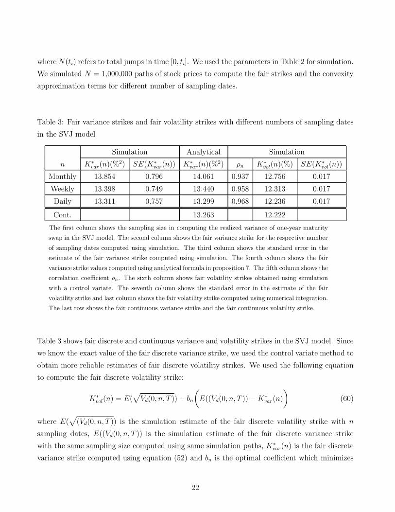
Table 3: Fair variance strikes and fair volatility strikes with different numbers of sampling dates

in the SVJ model

Simulation Analytical Simulation

n K∗var(n)(%2) SE(K∗

var(n)) K∗var(n)(%2) ρn K∗

vol(n)(%) SE(K∗vol(n))

Monthly 13.854 0.796 14.061 0.937 12.756 0.017

Weekly 13.398 0.749 13.440 0.958 12.313 0.017

Daily 13.311 0.757 13.299 0.968 12.236 0.017

Cont. 13.263 12.222

The first column shows the sampling size in computing the realized variance of one-year maturity

swap in the SVJ model. The second column shows the fair variance strike for the respective number

of sampling dates computed using simulation. The third column shows the standard error in the

estimate of the fair variance strike computed using simulation. The fourth column shows the fair

variance strike values computed using analytical formula in proposition 7. The fifth column shows the

correlation coefficient ρn. The sixth column shows fair volatility strikes obtained using simulation

with a control variate. The seventh column shows the standard error in the estimate of the fair

volatility strike and last column shows the fair volatility strike computed using numerical integration.

The last row shows the fair continuous variance strike and the fair continuous volatility strike.

Table 3 shows fair discrete and continuous variance and volatility strikes in the SVJ model. Since

we know the exact value of the fair discrete variance strike, we used the control variate method to

obtain more reliable estimates of fair discrete volatility strikes. We used the following equation

to compute the fair discrete volatility strike:

K∗vol(n) = E(

√Vd(0, n, T )) − bn

(E((Vd(0, n, T )) − K∗

var(n)

)(60)

where E(√

(Vd(0, n, T )) is the simulation estimate of the fair discrete volatility strike with n

sampling dates, E((Vd(0, n, T )) is the simulation estimate of the fair discrete variance strike

with the same sampling size computed using same simulation paths, K∗var(n) is the fair discrete

variance strike computed using equation (52) and bn is the optimal coefficient which minimizes

22

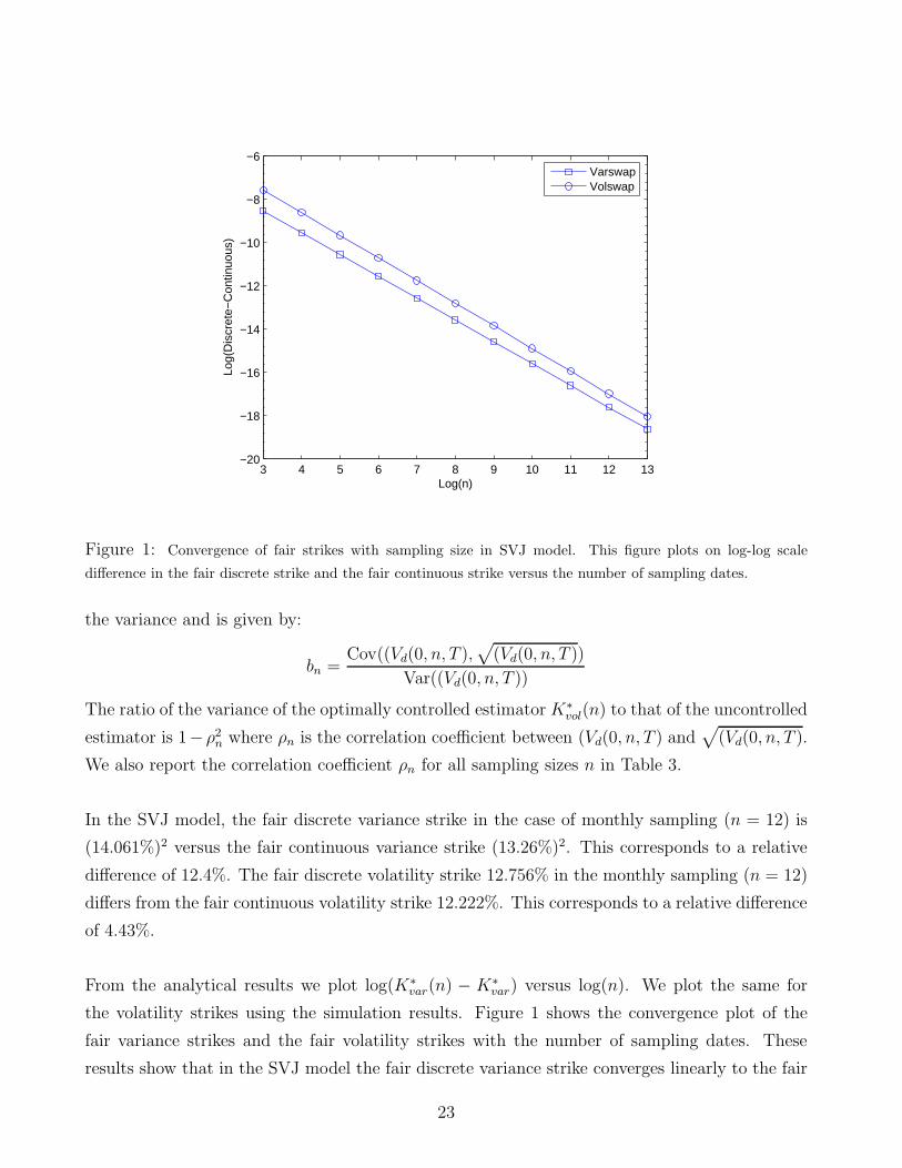
3 4 5 6 7 8 9 10 11 12 13−20

−18

−16

−14

−12

−10

−8

−6

Log(n)

Log(

Dis

cret

e−C

ontin

uous

)

VarswapVolswap

Figure 1: Convergence of fair strikes with sampling size in SVJ model. This figure plots on log-log scale

difference in the fair discrete strike and the fair continuous strike versus the number of sampling dates.

the variance and is given by:

bn =Cov((Vd(0, n, T ),

√(Vd(0, n, T ))

Var((Vd(0, n, T ))

The ratio of the variance of the optimally controlled estimator K∗vol(n) to that of the uncontrolled

estimator is 1− ρ2n where ρn is the correlation coefficient between (Vd(0, n, T ) and

√(Vd(0, n, T ).

We also report the correlation coefficient ρn for all sampling sizes n in Table 3.

In the SVJ model, the fair discrete variance strike in the case of monthly sampling (n = 12) is

(14.061%)2 versus the fair continuous variance strike (13.26%)2. This corresponds to a relative

difference of 12.4%. The fair discrete volatility strike 12.756% in the monthly sampling (n = 12)

differs from the fair continuous volatility strike 12.222%. This corresponds to a relative difference

of 4.43%.

From the analytical results we plot log(K∗var(n) − K∗

var) versus log(n). We plot the same for

the volatility strikes using the simulation results. Figure 1 shows the convergence plot of the

fair variance strikes and the fair volatility strikes with the number of sampling dates. These

results show that in the SVJ model the fair discrete variance strike converges linearly to the fair

23

continuous variance strike with the number of sampling dates, consistent with Proposition 7.

We determine the convergence rate of the fair discrete volatility strike to the fair continuous

volatility strike numerically using regression. The regression equation of the volatility strike is

log(K∗vol(n) − K∗

vol) = −1.046 log(n) − 4.428 R2 = 0.99 (61)

These results show that in SVJ model the fair discrete volatility strike converges linearly to the

fair continuous volatility strike with sampling size.

Table 4: Approximation of the fair volatility strike using the convexity correction formula in the

SVJ model

Convexity 3rd 4th Excess K∗vol(n)(%) K∗

vol(n)(%)

n correction(cc) order order Prob.(p) using cc correct value Diff (%)

Monthly 2.980 12.759 99.433 0.061 10.874 12.756 1.882

Weekly 2.915 12.488 97.879 0.062 10.483 12.313 1.830

Daily 3.039 13.454 122.090 0.072 10.272 12.131 1.859

The first column shows the number of sampling dates in computing the realized variance of one-year maturity

volatility swap. The second column shows the convexity correction term (28) with the different number of sampling

dates. The third and fourth columns show the 3rd and 4th order term in equation (30). The fifth column shows

the excess probability (29). The sixth column column shows the fair volatility strike computed using convexity

correction formula. The seventh column shows the fair volatility strike computed using simulation and the last

column shows the difference between the fair volatility strike computed using the simulation in Table 3 and the

convexity correction formula (28).

Table 4 shows the results of computing the fair volatility strike by the convexity correction for-

mula. The excess probability p from (29) is not equal to zero and the 3rd and 4th order terms in

equation (30) are comparable in magnitude with convexity correction term. We can see from the

last column that the differences between the exact fair volatility strike computed using numeri-

cal integration and the approximation using the convexity correction formula is quite significant,

i.e., the convexity correction formula does not provide a good approximation to the fair volatility

strike in the SVJ model.

24

6.3 Discrete strikes and convexity corrections in different models

Next we analyze fair variance strikes and fair volatility strikes in different models with different

sampling sizes. Table 5 shows these results. In these results we compute discrete and continuous

variance strikes using analytical formulas in all four models. We compute the fair continuous

volatility strike using numerical integration in all four models. The discrete volatility strike is

computed using numerical integration in the BS and J models and using simulation with control

variates in the SV and SVJ models. It can be seen from the results that the fair volatility strike

is less than the square root of the fair variance strike since the payoff of the volatility swap is

concave in the realized variance. This is true for all models and all sampling sizes except for

continuous sampling in the Black-Scholes model in which case they are equal. Even though fair

continuous variance strikes are identical in all models, the fair volatility strikes in SVJ model are

less compared to the SV and J model, i.e., there is more convexity value in the SVJ model. Fair

discrete strikes under monthly and weekly sampling are considerably different than under con-

tinuous sampling. Formulas and results derived for idealized contracts with continuous sampling

should be applied with caution to instruments which use discrete sampling.

Table 5: Comparison of fair variance strikes and fair volatility strikes in different models

Sampling K∗var(%

2) K∗vol(%)

Size (n) BS SV J SVJ BS SV J SVJ

Monthly 13.86 13.92 13.87 14.06 13.54 13.40 12.80 12.76

Weekly 13.33 13.41 13.39 13.44 13.33 13.14 12.56 12.31

Daily 13.27 13.29 13.29 13.30 13.28 13.10 12.50 12.24

Continuous 13.26 13.26 13.26 13.26 13.26 13.09 12.48 12.22

The first column shows the number of sampling dates. Then next four columns show

fair variance strikes in the Black-Scholes (BS), the Heston stochastic volatility (SV), the

Merton jump-diffusion model (J) and stochastic volatility model with jumps (SVJ) respec-

tively. The last three columns show fair volatility strikes in respective models.

Next we compute variance strikes and volatility strikes with an alternative definition of the re-

alized variance in equation (1). All the results so far were computed for a maturity of one year

and with m = n − 1 in the realized variance definition specified in equation (1). We have seen

that with this definition (m = n − 1) discrete variance strikes are different than the continu-

25

Table 6: Comparison of fair variance strikes with an alternative definition of realized variance

and with maturities in the SVJ model

Sampling 1 month 6 months 1 year 30 years

Size n m = n − 1 m = n m = n − 1 m = n m = n − 1 m = n m = n − 1 m = n

Monthly 14.59 13.32 14.06 13.46 13.71 13.69

Weekly 14.74 12.76 13.31 13.05 13.44 13.31 13.65 13.64

Daily 12.56 12.35 13.04 12.99 13.30 13.27 13.63 13.63

Continuous 12.29 12.97 13.26 13.63

The first column shows the sampling size. The first row shows the maturity of the variance strike. The columns

m = n− 1 refers to the variance strike computed when m = n− 1 in the realized variance definition in equation

(1). The columns m = n refers to the variance strike computed when m = n in the realized variance definition

in equation (1).

ous variance strikes. Table 6 shows the variance strikes computed using two definitions of the

realized variance and with different maturities in the SVJ model. The results show that using

m = n in the definition of realized variance removes the effect of discrete sampling in the fair

variance strike. The effect of discrete sampling is more pronounced for shorter maturity swaps.

In practice, the typical maturity of swaps varies from one month to 30 years with one month

being most the popular. In practice most of the contracts sampling is done daily or weekly

and sometimes monthly. Using these parameters there is a 27 basis point difference between

one-month fair variance strikes using discrete sampling (daily) and continuous sampling. The

effect of discreteness decreases as maturity increases.

Next we analyze the accuracy of the convexity correction formula in computing volatility strikes

across different models. The difference in the fair volatility strike and the square root of the

fair variance strike is called the convexity value. Table 7 shows fair volatility strikes computed

using the convexity correction formula and true fair volatility strikes in all models. The convex-

ity correction formula works well in the Black-Scholes model and but tends to perform poorly

in the Heston stochastic volatility model and even worse in models with jumps (J and SVJ). It

can be seen from the results that the convexity value depends on the model and the sampling size.

26

Table 7: Comparison of fair volatility strikes and approximations using the convexity correction

formula in different models

Sampling BS K∗vol(%) SV K∗

vol(%) J K∗vol(%) SVJ K∗

vol(%)

Size n cc true cc true cc true cc true

Monthly 13.54 13.54 13.31 13.40 10.99 12.80 10.87 12.76

Weekly 13.33 13.33 13.12 13.14 10.61 12.56 10.48 12.31

Daily 13.28 13.28 13.09 13.10 10.44 12.50 10.27 12.13

The first column shows the number of sampling dates. Then next two columns show

fair volatility strikes in the Black-Scholes (BS) model computed using the convexity

correction formula and true fair volatility strikes. The fourth and the fifth columns

provide results in the Heston stochastic volatility (SV) and the sixth and seventh

columns give results for the Merton jump-diffusion (J) model and last two columns

give results for the stochastic volatility model with jumps (SVJ).

7 Conclusion

In this paper we study the pricing of variance swaps and volatility swaps in four financial models.

We derive analytical formulas for fair discrete variance strikes in the Black-Scholes model, the

Heston stochastic volatility model, the Merton jump-diffusion model and the Bates and Scott

stochastic volatility with jumps model. We investigate the effect of discrete sampling and jumps

on fair variance strikes. The effect of jumps depends on direction and magnitude of jumps,

e.g., the one-month discrete variance strike can be significantly different from the continuous fair

variance strike when the underlying has negative jumps. We also present an argument to show

that the convexity correction formula to approximate fair volatility strikes may not provide good

estimates in jump-diffusion models. We present numerical approaches to compute fair volatility

strikes. In particular we compute fair discrete volatility strikes from numerical integration and

Monte Carlo simulation techniques. We also show that in all models fair discrete variance and

volatility strikes converge linearly to fair continuous variance and volatility strikes, respectively,

as the sampling size increases.

27

References

Bates, D. (1996), ‘Jump and stochastic volatility: Exchange rate processes implict in deutche

mark in options’, Review of Financial Studies 9, 69–107.

Broadie, M. and Jain, A. (2007), Vix index and vix futures. Working paper, Columbia Business

School.

Broadie, M. and Jain, A. (2008), ‘Pricing and hedging of volatility derivatives’, The Journal of

Derivatives 15(3), 7–24.

Brockhaus, O. and Long, D. (2000), ‘Volatility swaps made simple’, Risk 19(1), 92–95.

Buehler, H. (2006), ‘Consistent variance curve models’, Finance and Stochastics 10(2), 178–203.

Cairns, A. (2000), ‘Interest rate models: An introduction’. Princeton University Press.

Carr, P., Geman, H., Madan, D. and Yor, M. (2005), ‘Pricing options on realized variance’,

Finance and Stochastics 9(4), 453–475.

Carr, P. and Lee, R. (2005), Robust replication of volatility derivatives. Working paper, Courant

Institute and University of Chicago, http://math.nyu.edu/research/carrp/research.html.

Carr, P. and Wu, L. (2006), ‘A tale of two indices’, Journal of Derivatives 13, 13–29.

Demeterfi, K., Derman, E., Kamal, M. and Zou, J. (1999), ‘A guide to volatility and variance

swaps’, Journal of Derivatives 4, 9–32.

Derman, E. and Kani, I. (1994), ‘Riding on a smile’, RISK magazine 7, 32–39.

Derman, E., Kani, I. and Zou, J. Z. (1996), ‘The local volatility surface unlocking the information

in index option prices’, Financial Analysts Journal 52(4), 25–36.

Detemple, J. B. and Osakwe, C. (2000), ‘The valuation of volatility options’, European Finance

Review 4(1), 21–50.

Duffie, D., Pan, J. and Singleton, K. (2000), ‘Transform analysis and asset pricing for affine jump

diffusions’, Econometrica 68, 1343–1376.

Gatheral, J. (2006), ‘The volatility surface: A practitioner’s guide’. John Wiley & Sons, Inc.

28

Heston, S. (1993), ‘A closed form solution of options with stochastic volatility with applications

to bond and currency options’, The Review of Financial Studies 6(2), 327–343.

Hull, J. C. and White, A. (1987), ‘The pricing of options on assets with stochastic volatility’,

Journal of Finance 42, 281–300.

Jacod, J. and Protter, P. (1998), ‘Asymptotic error distributions for the euler method for stochas-

tic difefrential equations’, The Annals of Probability 26(1), 267–307.

Javaheri, A., Wilmott, P. and Haug, E. (2002), Garch and volatility swaps. Working Paper,

http://www.wilmott.com.

Lipton, A. (2000), ‘Mathematical methods for foreign exchange: A financial engineer’s approach’.

World Scientific.

Little, T. and Pant, V. (2001), ‘A finite difference method for the valuation of variance swaps’,

Journal of Computational Finance 5(1), 81–103.

Meddahi, N. (2002), ‘A theoretical comparison between integrated and realized volatility’, Jour-

nal of Applied Economics 17, 479–508.

Merton, R. C. (1973), ‘Theory of rational option pricing’, Bell Journal of Economic Management

Science 4, 141–183.

Schobel, R. and Zhu, J. (1999), ‘Stochastic volatility with an Ornstein Uhlenbeck process: An

extension’, European Finance Review 3(1), 23–46.

Schurger, K. (2002), Laplace transforms and suprema of stochastic processes. In: K. Sandmann,

P. J. Schonbucher (Ed.), Advances in Finance and Stochastics. Springer, Berlin, pp.287-293.

Scott, L. (1997), ‘Pricing stock options in a jump-diffusion model with stochastic volatility and

interest rates: Applications of fourier inversion methods’, Mathematical Finance 7(4), 413–

424.

Sepp, A. (2008), ‘Pricing options on realized variance in the heston model with jumps in returns

and volatility’, Journal of Computational Finance 11(4), 37–70.

Stein, E. M. and Stein, J. (1991), ‘Stock price distribution with stochastic volatility: An analytic

approach’, Review of Financial Studies 4, 727–752.

29

A

Proof of Proposition 1: The Laplace transform of continuous realized variance can be ex-

pressed as

E(exp(−sVc(0, T ))) = E(exp(−s(σ2 +1

T

N(T )∑i=1

(ln(Yi))2)))

= exp(−sσ2)E

(E

(1

T

n∑i=1

(ln(Yi))2|N(T ) = n

))(A-1)

where second equality follows by taking an expectation conditional on a Poisson random variable,

N(T ) = n. Since ln(Yi) ∼ N(a, b2), the inner expectation can be computed as:

E(exp(−sVc(0, T ))) = exp(−sσ2)E

(exp

(−sna2

T+2sb2

)(1 + 2sb2

T)

n2

)(A-2)

We can compute the outer expectation as follows:

E(exp(−sVc(0, T ))) = exp(−sσ2)∞∑

n=0

exp(−λT )(λT )n

n!

(exp

(−sna2

T+2sb2

)(1 + 2sb2

T)

n2

)(A-3)

Simplifying the infinite sum gives

E(exp(−sVc(0, T ))) = exp(−sσ2) exp(−λT ) exp

(λT exp( −sa2

T+2sb2)√

(1 + 2sb2

T)

)

= exp

(− sσ2 + λT

(exp( −sa2

T+2sb2)√

(1 + 2sb2

T)− 1

))�

Proof of Proposition 2: Applying Ito’s lemma in the jump-diffusion model (31) and integrating

from ti to ti+1 gives

ln

(Si+1

Si

)= (r − λm − 1

2σ2)Δt + σ

√ΔtZi+1 + ln

( nj∏j=1

Yj

)(A-4)

where nj is number of jumps in the stock price during time ti+1 − ti. Squaring equation (A-4)

on both sides and summing from time 0 to time n − 1 we get

n−1∑i=0

(ln

(Si+1

Si

))2

=

n−1∑i=0

[(r − λm − 1

2σ2

)2

Δt2 + σ2ΔtZ2i+1 + 2σ(r − λm − 1

2σ2)Δt

32 Zi+1

+

( nj∑j=1

ln Yj

)2

+ 2

(r − λm − 1

2σ2

)Δt

( nj∑j=1

ln Yj

)+ 2σΔt

12 Zi+1

( nj∑j=1

ln Yj

)](A-5)

30

The fair discrete variance strike can be calculated by dividing equation (A-5) on both sides by

(n − 1)Δt and taking expectation under the risk-neutral measure:

K∗var(n) = E

[Vd(0, n, T )

]= E

[(r − λm − 1

2σ2

)2

Δtn

n − 1+ σ2Z2

i+1

n

n − 1

+2σ(r − λm − 1

2σ2)Δt

12 Zi+1

n

n − 1+ (Σ

nj

j=1 ln Yj)2 n

(n − 1)Δt

+2(r − λm − 1

2σ2)(Σ

nj

j=1 ln Yj)n

n − 1

+2σZi+1(Σnj

j=1 ln Yj)n

(n − 1)Δt12

](A-6)

Using properties of the normal and Poisson distributions

E(Zi) = 0 E[Z2i+1] = 1 E

[ nj∑j=1

ln Yj

]= aλΔt

E

[ nj∑j=1

ln Yj

]2

= b2E[nj ] + a2(E(nj)2) = (a2 + b2)(λΔt) + (λΔt)2a2

Substituting these in equation (A-6) we get

K∗var(n) = (r − λm − 1

2σ2)2 T

n − 1+ σ2 n

n − 1+

(a2 + b2)λn

n − 1+

a2λ2T

n − 1+ 2(r − λm − 1

2σ2)

aλT

n − 1(A-7)

The previous expression gives the fair discrete variance strike. Rearranging terms gives (38). �

Proof of Proposition 3: The Laplace transform of discrete realized variance is

E

(exp(−sVd(0, n, T ))

)= E

(exp

(−s∑n−1

i=0

(ln

(Si+1

Si

))2

(n − 1)Δt

))

= E

(E

(exp

(−s

( ∑n−1i=0 ln

(Si+1

Si

))2

(n − 1)Δt

)∣∣∣∣N(0), N(t1)...., N(T ))

)

= E

( n−1∏0

E

(exp

(−s

(ln

(Si+1

Si

))2

(n − 1)Δt

)∣∣∣∣N(0), N(t1)...., N(T ))

)(A-8)

31

The third equality follows since a Poisson process has stationary and independent increments

where

ln

(Si+1

Si

)= (r − λm − 1

2σ2)Δt + σ

√ΔtZi+1 +

ni∑j=1

(ln(Yj)

)(A-9)

and ni is number of jumps in the stock price during the time ti+1 − ti. The random variables

ni are independent and identically distributed with Poisson rate λΔt for each i = 0, 1, ..., n − 1.

Since ln(Yj) ∼ N(a, b2) the distribution of log return given ni jumps is

ln

(Si+1

Si

)∼ N((r − λm − 1

2σ2)Δt + ani, σ

2Δt + b2ni) (A-10)

The inner expectation in equation (A-8) can be solved using property (A-10):

E

(exp(−sVd(0, n, T ))

)= E

( n−1∏i=0

(exp

(−s((r−λm− 1

2σ2)Δt+ani)

2

(n−1)Δt+2s(σ2Δt+b2ni)

)√

(1 + 2s(σ2Δt+b2ni)(n−1)Δt

)

))

=

( ∞∑ni=0

exp(−λΔt(λΔt)ni)

ni!

(exp

(−s((r−λm− 1

2σ2)Δt+ani)2

(n−1)Δt+2s(σ2Δt+b2ni)

)√

(1 + 2s(σ2Δt+b2ni)(n−1)Δt

)

))n

(A-11)

The second equality follows since ni are independent. �

Proof of Proposition 4: The Laplace transform of∫ T

0vsds is given by (Cairns 2000)

E0[e−s 1

T

R T0

vtdt | v(0) = v0] = exp[A(T, s) − B(T, s)v0] (A-12)

where

A(T, s) =2κθ

σ2v

log

(2γ(s)e

(γ(s)+κ)T2

(γ(s) + κ)(e(γ(s))T − 1) + 2γ(s)

)B(T, s) =

2s(e(γ(s))T − 1)

T (γ(s) + κ)(e(γ(s))T − 1) + 2γ(s)

γ(s) =

√κ2 + 2

σ2vs

T

From the Laplace transform of∫ T

0vsds we can derive the first moment:

E

[ ∫ T

t

vsds

]= − d

dν

(EQ[e−ν

R Tt

vsds | v(t) = vt]

)∣∣∣∣(ν=0)

= θ(T − t) +vt − θ

κ(1 − e−κ(T−t))

32

which proves (42). �

Proof of Proposition 5:

The discrete variance strike can be derived as follows. Applying Ito’s lemma to ln(St) in equation

(40) we get

d(lnSt) =

(r − 1

2vt

)dt +

√vt

(ρdW 1

t +√

1 − ρ2dW 2t

)(A-13)

Integrating equation (A-13) from ti to ti+1 squaring and taking expectations in the risk-neutral

measure we get

E

[ln

(Sti+1

Sti

)]2

= E

[ ∫ ti+1

ti

(r − 1

2vt)dt +

∫ ti+1

ti

√vt(ρdW 1

t +√

1 − ρ2dW 2t )

]2

= E

[(rΔt −

∫ ti+1

ti

1

2vtdt

)2

+

( ∫ ti+1

ti

√vt(ρdW 1

t +√

1 − ρ2dW 2t )

)2

+2

(rΔt −

∫ ti+1

ti

1

2vtdt

)( ∫ ti+1

ti

√vt(ρdW 1

t +√

1 − ρ2dW 2t )

)]Applying Ito’s isometry rule on second term and simplifying other terms we get:

E

[ln

(Sti+1

Sti

)]2

= (rΔt)2 +1

4E

[( ∫ ti+1

ti

vtdt

)2]− (rΔt)E

[( ∫ ti+1

ti

vtdt

)]+E

[ ∫ ti+1

ti

vtdt

]+ 2rΔtE

[ ∫ ti+1

ti

√vt(ρdW 1

t +√

1 − ρ2dW 2t )

]−E

[( ∫ ti+1

ti

vtdt

)( ∫ ti+1

ti

√vt(ρdW 1

t +√

1 − ρ2dW 2t )

)](A-14)

The variance process has the following properties:

E(vt) = exp(−kt)(v0 − θ) + θ

E(vtvs) = σv2 exp(−k(t + s)

(exp(ks) − 1

k(v0 − θ) +

exp(2ks) − 1

2k(θ)

)+ exp(−k(t + s))(v0 − θ)2 + exp(−kt)(v0 − θ)θ + exp(−ks)(v0 − θ)θ + θ2

E

[ ∫ ti+1

ti

√vt(ρdW 1

t +√

1 − ρ2dW 2t )

]= 0 (A-15)

Using properties (A-15) we solve for the last term in equation (A-14):

E

[( ∫ ti+1

ti

vtdt

)( ∫ ti+1

ti

√vt(ρdW 1

t +√

1 − ρ2dW 2t )

)]= E

[( ∫ ti+1

ti

vtdt

)( ∫ ti+1

ti

√vtρdW 1

t

)]+ E

[( ∫ ti+1

ti

vtdt

)( ∫ ti+1

ti

√vt

√1 − ρ2dW 2

t

)](A-16)

33

The 2nd expectation in equation (A-16) is zero and first term can be rewritten using (41) as

E

[ρ

σv

( ∫ ti+1

ti

vtdt

)(vti+1

− vti −∫ ti+1

ti

κ(θ − vt)dt)

]= E

[ρ

σv

( ∫ ti+1

ti

vtdt

)(vti+1

− vti

)]− ρ

σvκθΔtE

( ∫ ti+1

ti

vtdt

)+

ρκ

σvE

( ∫ ti+1

ti

∫ ti+1

ti

vtvsdtds

)(A-17)

Next we compute the first term in equation (A-17):

E

[( ∫ ti+1

ti

vtdt

)(vti

)]=

(1 − exp(−κti))σ2v(v0 − θ)

κ2

(+ exp(−κti) − exp(−κti+1)

)+

σ2vθ

2κ2

((exp(κti) − exp(−κti))(− exp(−κti+1) + exp(−κti))

)+

exp(−κti)(v0 − θ)2

κ

(− exp(−κti+1) + exp(−κti)

)+

(v0 − θ)θ

κ

(− exp(−κti+1) + exp(−κti)

)+ exp(−κti)(v0 − θ)θΔt + θ2Δt

(A-18)

E

[( ∫ ti+1

ti

vti+1vtdt

)]=

exp(−κti+1)σ2v(v0 − θ)

κ2

(κΔt − exp(−κti) + exp(−κti+1)

)+

exp(−κti+1)σ2vθ

2κ2

(exp(κti+1) − exp(κti) + exp(−κti+1) − exp(−κti)

)+

exp(−κti+1)(v0 − θ)2

κ

(− exp(−κti+1) + exp(−κti)

)+

(v0 − θ)θ

κ

(− exp(−κti+1) + exp(−κti)

)+ exp(−κti+1)(v0 − θ)θΔt + θ2Δt

(A-19)

Subtracting equation (A-18) from (A-19) and simplifying we get

E

[( ∫ ti+1

ti

vtdt

)(vti+1

− vti

)]=

σ2v(v0 − θ)

κ2

(exp(−κti+1)(1 + κΔt − exp(κΔt))

)−

(σ2

v(θ − 2v0)

2κ2+

(v0 − θ)2

κ

)(exp(−2κti)

(1 − exp(−κΔt)

)2)+(v0 − θ)θΔt

(exp(−κti+1)

(1 − exp(κΔt)

))(A-20)

34

Summing equation (A-20) from time 0 to time n − 1 we get

n−1∑i=0

E

[( ∫ ti+1

ti

vtdt

)(vti+1

− vti

)]=

σ2v(v0 − θ)

κ2

((1 + κΔt − exp(κΔt))

)(1 − exp(−κT )

−1 + exp(κTn

)

)−

(σ2

v(θ − 2v0)

2κ2+

(v0 − θ)2

κ

)((1 − exp(−2κT )

1 − exp(−2κTn

)

)(

1 − exp(−κΔt)

)2)+(v0 − θ)θΔt

((1 − exp(−κT )

−1 + exp(κTn

)

)(1 − exp(κΔt)

))(A-21)

All terms on right hand side of equation (A-21) are of the order O(Δt). We expand the terms

to show this:

((1 + κΔt − exp(κΔt))

)(1 − exp(−κT )

−1 + exp(κTn

)

)≡ −

((κΔt)2

2+

(κΔt)3

6+ ...

)(1 − exp(−κT )

(κΔt) + (κΔt)2

2+ ...

)≡ O(Δt)

(1 − exp(−2κT )

1 − exp(−2κTn

)

)(1 − exp(−κΔt)

)2

≡(

1 − exp(−2κT )

(2κΔt) + (2κΔt)2

2+ ...

)((κΔt) − (κΔt)2

2+ ...

)2

≡ O(Δt)

Δt

((1 − exp(−κT )

−1 + exp(κTn

)

)(1 − exp(κΔt)

))≡ O(Δt)

Hence the left hand side of the equation (A-21) is of the order O(Δt).

Next we compute the last term in equation (A-17):

n−1∑i=0

E

[( ∫ ti+1

ti

vtdt

)2]=

n−1∑i=0

E

( ∫ ti+1

ti

∫ ti+1

ti

vtvsdtds

)

=n−1∑i=0

Var

( ∫ ti+1

ti

vsds

)+

n−1∑i=0

(E

( ∫ ti+1

ti

vsds

))2

(A-22)

35

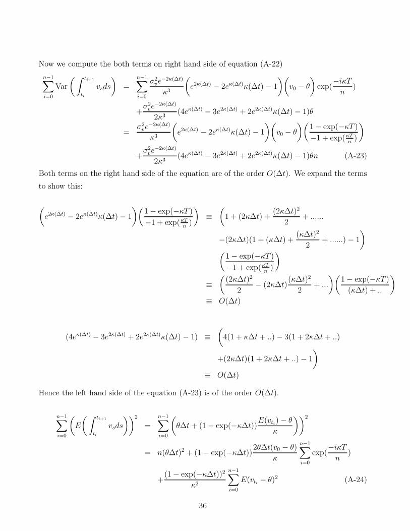
Now we compute the both terms on right hand side of equation (A-22)

n−1∑i=0

Var

(∫ ti+1

ti

vsds

)=

n−1∑i=0

σ2ve

−2κ(Δt)

κ3

(e2κ(Δt) − 2eκ(Δt)κ(Δt) − 1

)(v0 − θ

)exp(

−iκT

n)

+σ2

ve−2κ(Δt)

2κ3(4eκ(Δt) − 3e2κ(Δt) + 2e2κ(Δt)κ(Δt) − 1)θ

=σ2

ve−2κ(Δt)

κ3

(e2κ(Δt) − 2eκ(Δt)κ(Δt) − 1

)(v0 − θ

)(1 − exp(−κT )

−1 + exp(κTn

)

)+

σ2ve

−2κ(Δt)

2κ3(4eκ(Δt) − 3e2κ(Δt) + 2e2κ(Δt)κ(Δt) − 1)θn (A-23)

Both terms on the right hand side of the equation are of the order O(Δt). We expand the terms

to show this:

(e2κ(Δt) − 2eκ(Δt)κ(Δt) − 1

)(1 − exp(−κT )

−1 + exp(κTn

)

)≡

(1 + (2κΔt) +

(2κΔt)2

2+ ......

−(2κΔt)(1 + (κΔt) +(κΔt)2

2+ ......) − 1

)(

1 − exp(−κT )

−1 + exp(κTn

)

)≡

((2κΔt)2

2− (2κΔt)

(κΔt)2

2+ ...

)(1 − exp(−κT )

(κΔt) + ..

)≡ O(Δt)

(4eκ(Δt) − 3e2κ(Δt) + 2e2κ(Δt)κ(Δt) − 1) ≡(

4(1 + κΔt + ..) − 3(1 + 2κΔt + ..)

+(2κΔt)(1 + 2κΔt + ..) − 1

)≡ O(Δt)

Hence the left hand side of the equation (A-23) is of the order O(Δt).

n−1∑i=0

(E

( ∫ ti+1

ti

vsds

))2

=n−1∑i=0

(θΔt + (1 − exp(−κΔt))

E(vti) − θ

κ

))2

= n(θΔt)2 + (1 − exp(−κΔt))2θΔt(v0 − θ)

κ

n−1∑i=0

exp(−iκT

n)

+(1 − exp(−κΔt))2

κ2

n−1∑i=0

E(vti − θ)2 (A-24)

36

n−1∑i=0

E(vti − θ)2 =

n−1∑i=0

E(vti)2 − nθ2 − 2θ(v0 − θ)

n−1∑i=0

exp(−iκT

n) (A-25)

n−1∑i=0

E(vti)2 =

((v0 − θ)2 − (v0 − θ)σ2

v

κ− σ2

vθ

2κ

) n−1∑i=0

exp(−i2κT

n)

+

(2(v0 − θ)θ +

(v0 − θ)σ2v

κ

) n−1∑i=0

exp(−iκT

n) + n(θ2 +

σ2vθ

2κ) (A-26)

All terms on right hand side of equation (A-24) are of the order O(Δt). We expand the terms

to show this:

(1 − exp(−κΔt))Δtn−1∑i=0

exp(−iκT

n) ≡ (1 − exp(−κΔt))Δt

(1 − exp(−κT )

1 − exp(−κΔt)

)≡ O(Δt)

(1 − exp(−κΔt))2

n−1∑i=0

E(vti − θ)2 ≡ (1 − exp(−κΔt))2

( n−1∑i=0

E(vti)2

−nθ2 − 2θ(v0 − θ)

n−1∑i=0

exp(−iκT

n)

)≡ O(Δt)

Using equations (A-25) and (A-26) we can compute (A-24). Using equations (A-24) and (A-23)

we can compute (A-22). The fair discrete variance strike is the expectation of the discrete realized

variance

K∗var(n) = E[Vd(0, n, T )] = EQ

0

[∑n−1i=0 (ln(Si+1

Si))2

(n − 1)Δt

]Dividing equation (A-14) on both sides by (n − 1)Δt and summing from time 0 to time n − 1

37

we get

E[Vd(0, n, T )] =r2T

n − 1+

∑n−1i=0 E

( ∫ ti+1

ti

∫ ti+1

tivtvsdtds

)4(n − 1)Δt

−rE[∫ T

0vtdt]

(n − 1)+

nE[∫ T

0vtdt]

T (n − 1)+

ρκθE[∫ T

0vtdt]

(n − 1)σv

−∑n−1

i=0 E

(ρκ

∫ ti+1

ti

∫ ti+1

tivtvsdtds

)σv(n − 1)Δt

−∑n−1

i=0 E

[ρ

( ∫ ti+1

tivtdt

)(vti+1

− vti

)]σv(n − 1)Δt

(A-27)

This equation can be simplified as

E[Vd(0, n, T )] =1

TE[

∫ T

0

vtdt] +E[

∫ T

0vtdt]

T (n − 1)+

r2T

n − 1− rE[

∫ T

0vtdt]

(n − 1)

+ρκθE[

∫ T

0vtdt]

(n − 1)σv+

∑n−1i=0 E

( ∫ ti+1

ti

∫ ti+1

tivtvsdtds

)(n − 1)Δt

(1

4− ρκ

σv

)

−∑n−1

i=0 E

[ρ

( ∫ ti+1

tivtdt

)(vti+1

− vti

)]σv(n − 1)Δt

(A-28)

The last term in equation (A-28) is given by equation (A-21). The second last term in equation

(A-28) is given by equation (A-22). All terms except the first one on right hand side in expression

(A-28) is of the order O(Δt) or O( 1n) . The first term on the right hand side is the fair continuous

variance strike, i.e., 1TE[

∫ T

0vtdt] = K∗

var. It is given by equation (42). Hence, the discrete variance

strike can be represented as:

K∗var(n) = K∗

var + g(r, ρ, σv, κ, θ, n) (A-29)

where

g(r, ρ, σv, κ, θ, n) =r2T

n − 1+

1

TE

( ∫ T

0

vtdt

)(1

(n − 1)− rT

(n − 1)+

ρκθT

(n − 1)σv

)

+

∑n−1i=0 E

( ∫ ti+1

ti

∫ ti+1

tivtvsdtds

)(n − 1)Δt

(1

4− ρκ

σv

)

−∑n−1

i=0 E

[ρ

( ∫ ti+1

tivtdt

)(vti+1

− vti

)]σv(n − 1)Δt

(A-30)

38

g(r, ρ, σv, κ, θ, n) = O

(1

n

)(A-31)

Hence

K∗var(n) → E

[1

T

∫ T

0

vtdt

]= K∗

var as Δt → 0 � (A-32)

Proof of Proposition 7: The discrete variance strike can be derived as follows. Applying Ito’s

lemma to ln(St) in equation (46) and integrating from ti to ti+1 gives

ln

(Si+1

Si

)=

∫ ti+1

ti

(r − λm − 1

2vt)dt +

∫ ti+1

ti

√vt(ρdW 1

t +√

1 − ρ2dW 2t ) + ln

( nj∏j=1

Yj

)(A-33)

where nj is number of jumps in the stock price during time ti+1 − ti. Squaring equation (A-33),

summing from time 0 to time n− 1, dividing on both sides by (n − 1)Δt and taking expectation

under the risk-neutral measure we get

E

[ n−1∑i=0

1

(n − 1)Δt

(ln

(Sti+1

Sti

))2]

= En−1∑i=0

1

(n − 1)Δt

[((r − λm)Δt −

∫ ti+1

ti

1

2vtdt

)2

+

( ∫ ti+1

ti

√vt(ρdW 1

t +√

1 − ρ2dW 2t )

)2

+2

((r − λm)Δt −

∫ ti+1

ti

1

2vtdt

)( ∫ ti+1

ti

√vt(ρdW 1

t +√

1 − ρ2dW 2t )

)+

( nj∑j=1

lnYj

)2

+ 2

((r − λm)Δt −

∫ ti+1

ti

1

2vtdt

)( nj∑j=1

ln Yj

)

+2

( ∫ ti+1

ti

√vt(ρdW 1

t +√

1 − ρ2dW 2t )

)( nj∑j=1

ln Yj

)](A-34)

The first two lines of expressions on the right hand side of equation (A-34) can be computed

using Proposition 5 and it is equal to

1

TE

[ ∫ T

0

vtdt

]+ g(r − λm, ρ, σv, κ, θ, n) (A-35)

and using equation(A-31) we get

g(r − λm, ρ, σv, κ, θ, n) = O

(1

n

)(A-36)

39

The last two lines of expressions on the right hand side of equation (A-34) can be computed

using Proposition 2 and it is equal to

λ(a2 + b2) +

λ(a2 + b2) + λ2a2T + λa

(2(r − λm)T − E[

∫ T

0vtdt]

)n − 1

(A-37)

where E[∫ T

0vtdt] is given by equation (42). Hence using equations (A-34), (A-35) and (A-35)

the fair discrete variance strike is given by:

K∗var(n) = E

[Vd(0, n, T )

]= E

[ n−1∑i=0

1

(n − 1)Δtln

(Sti+1

Sti

)]2

=1

TE

[ ∫ T

0

vtdt

]+ λ(a2 + b2) + g(r − λm, ρ, σv, κ, θ, n)

+

λ(a2 + b2) + λ2a2T + λa

(2(r − λm)T − E[

∫ T

0vtdt]

)n − 1

(A-38)

Hence, the fair discrete variance strike can be represented as:

K∗var(n) = K∗

var + h(r, ρ, σv, κ, θ, m, b, n) (A-39)

where

K∗var = θ +

v0 − θ

κT(1 − e−κT ) + λ(a2 + b2) (A-40)

and

h(r, ρ, σv, κ, θ, m, b, n) = g(r − λm, ρ, σv, κ, θ, n)

+

λ(a2 + b2) + λ2a2T + λa

(2(r − λm)T − E[

∫ T

0vtdt]

)n − 1

(A-41)

h(r, ρ, σv, κ, θ, m, b, n) = O

(1

n

)(A-42)

40