Variance options, Skorokhod embeddings and … options, Skorokhod embeddings and Obstacle problems...
48
Transcript of Variance options, Skorokhod embeddings and … options, Skorokhod embeddings and Obstacle problems...
Variance options, Skorokhod embeddings andObstacle problems
Gonçalo dos Reis (joint work with H. Oberhauser)
TU Berlin
Oxford OMI, 04 Dez. 2012
I. Motivation from nance
II. Skorohod embedding problem and Root embedding
III. Root's barrier and Obstacle PDEs
1..1 From barrier to PDE2..2 From PDE to barrier

I. Financial Motivation: pricing exotic options
How to price? Standard approach
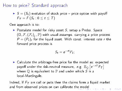
I S = (St) evolution of stock price price option with payoFT = F (St : 0 ≤ t ≤ T )
One approach is to:
I Postulate model for risky asset S , setup a Proba. Space(Ω,F , (Ft)t ,P) with usual assumps. carrying a price processP = (Pt)t for the liquid asset. With const. interest rate r theforward price process is
St = e−rtPt ;
I Calculate the arbitrage-free price for the model as: expectedpayo under the risk-neutral measure, .e.g. EQ
[e−rTFT
]where Q is equivalent to P and under which S is alocal-Martingale.
Indeed, if FT are call or puts then the claims form a liquid marketand from observed prices on can calibrate the model
How to price? Standard approach
I S = (St) evolution of stock price price option with payoFT = F (St : 0 ≤ t ≤ T )
One approach is to:
I Postulate model for risky asset S , setup a Proba. Space(Ω,F , (Ft)t ,P) with usual assumps. carrying a price processP = (Pt)t for the liquid asset. With const. interest rate r theforward price process is
St = e−rtPt ;
I Calculate the arbitrage-free price for the model as: expectedpayo under the risk-neutral measure, .e.g. EQ
[e−rTFT
]where Q is equivalent to P and under which S is alocal-Martingale.
Indeed, if FT are call or puts then the claims form a liquid marketand from observed prices on can calibrate the model
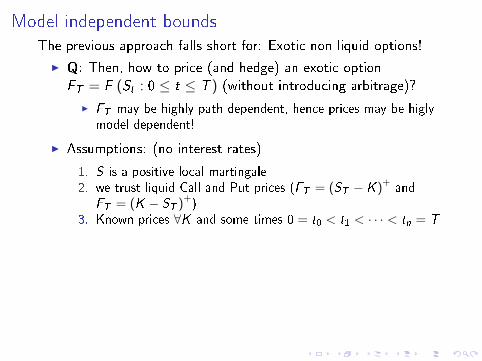
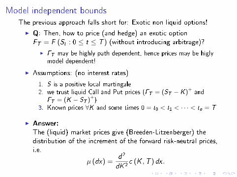
Model independent boundsThe previous approach falls short for: Exotic non-liquid options!
I Q: Then, how to price (and hedge) an exotic optionFT = F (St : 0 ≤ t ≤ T ) (without introducing arbitrage)?
I FT may be highly path dependent, hence prices may be higlymodel dependent!
I Assumptions: (no interest rates)
1. S is a positive local martingale2. we trust liquid Call and Put prices (FT = (ST − K )+ and
FT = (K − ST )+)3. Known prices ∀K and some times 0 = t0 < t1 < · · · < tn = T
I Answer:The (liquid) market prices give (Breeden-Litzenberger) thedistribution of the increment of the forward risk-neutral prices,i.e.
µ (dx) =d2
dK 2c (K ,T ) dx .
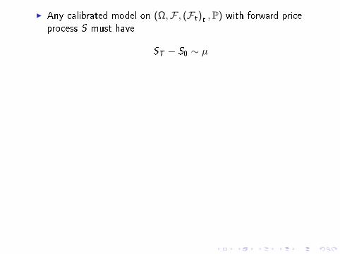
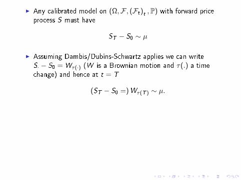
I Any calibrated model on (Ω,F , (Ft)t ,P) with forward priceprocess S must have
ST − S0 ∼ µ
I Assuming Dambis/Dubins-Schwartz applies we can writeS· − S0 = Wτ(·) (W is a Brownian motion and τ(.) a timechange) and hence at t = T
(ST − S0 =)Wτ(T ) ∼ µ.
Now, from the above we can conclude that all arbitragefree pricefor FT are in[infτE [F (Wt : t ∈ [0, τ ])] , sup
τE [F (Wt : t ∈ [0, τ ])]
]τ s.t. Wτ ∼ µ
I Bounds attained by St − S0 := Wτ?∧t/(T−t) with extremalsolution τ? of Skorohod problem Wτ? ∼ µ
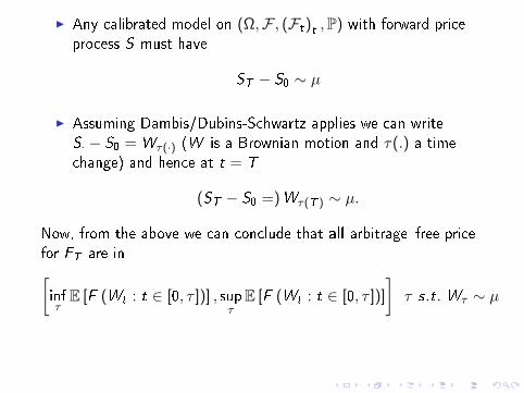
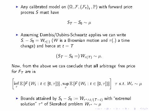
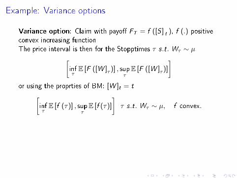
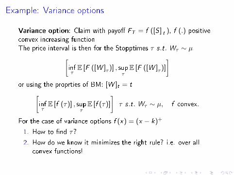
Example: Variance options
Variance option: Claim with payo FT = f ([S ]T
), f (.) positiveconvex increasing function
The price interval is then for the Stopptimes τ s.t. Wτ ∼ µ[infτE [F ([W ]τ )] , sup
τE [F ([W ]τ )]
]or using the proprties of BM: [W ]t = t[
infτE [f (τ)] , sup
τE [f (τ)]
]τ s.t. Wτ ∼ µ, f convex.
For the case of variance options f (x) = (x − k)+
1. How to nd τ?
2. How do we know it minimizes the right rule? i.e. over allconvex functions!
Example: Variance options
Variance option: Claim with payo FT = f ([S ]T
), f (.) positiveconvex increasing functionThe price interval is then for the Stopptimes τ s.t. Wτ ∼ µ[
infτE [F ([W ]τ )] , sup
τE [F ([W ]τ )]
]or using the proprties of BM: [W ]t = t[
infτE [f (τ)] , sup
τE [f (τ)]
]τ s.t. Wτ ∼ µ, f convex.
For the case of variance options f (x) = (x − k)+
1. How to nd τ?
2. How do we know it minimizes the right rule? i.e. over allconvex functions!
II. Skorokhod embedding problem
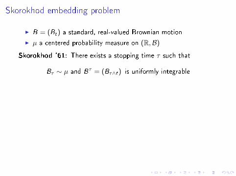
Skorokhod embedding problem
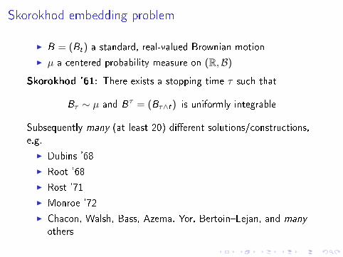
I B = (Bt) a standard, real-valued Brownian motion
I µ a centered probability measure on (R,B)
Skorokhod '61: There exists a stopping time τ such that
Bτ ∼ µ and Bτ = (Bτ∧t) is uniformly integrable
Subsequently many (at least 20) dierent solutions/constructions,e.g.
I Dubins '68
I Root '68
I Rost '71
I Monroe '72
I Chacon, Walsh, Bass, Azema, Yor, BertoinLejan, and many
others
Skorokhod embedding problem
I B = (Bt) a standard, real-valued Brownian motion
I µ a centered probability measure on (R,B)
Skorokhod '61: There exists a stopping time τ such that
Bτ ∼ µ and Bτ = (Bτ∧t) is uniformly integrable
Subsequently many (at least 20) dierent solutions/constructions,e.g.
I Dubins '68
I Root '68
I Rost '71
I Monroe '72
I Chacon, Walsh, Bass, Azema, Yor, BertoinLejan, and many
others
Many solutions!
I Dierent stopping times which solve the embedding of µ inBrownian motion,
I Criteria to choose a good solution
I Computable?I Natural?I Unique in some sense?
The nance says look at those that
I minimize over convex functions −→ Root embedding!
I maximize over convex function −→ Rost embedding!
Root's solution
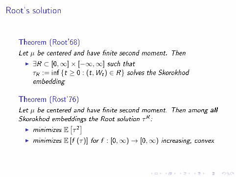
Theorem (Root'68)
Let µ be centered and have nite second moment. Then
I ∃R ⊂ [0,∞]× [−∞,∞] such that
τR := inf t ≥ 0 : (t,Wt) ∈ R solves the Skorokhodembedding
Theorem (Rost'76)
Let µ be centered and have nite second moment. Then among all
Skorokhod embeddings the Root solution τR :
I minimizes E[τ2]
I minimizes E [f (τ)] for f : [0,∞)→ [0,∞) increasing, convex
Root's solution
Theorem (Root'68)
Let µ be centered and have nite second moment. Then
I ∃R ⊂ [0,∞]× [−∞,∞] such that
τR := inf t ≥ 0 : (t,Wt) ∈ R solves the Skorokhodembedding
Theorem (Rost'76)
Let µ be centered and have nite second moment. Then among all
Skorokhod embeddings the Root solution τR :
I minimizes E[τ2]
I minimizes E [f (τ)] for f : [0,∞)→ [0,∞) increasing, convex
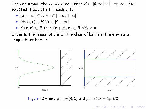
One can always choose a closed subset R ⊂ [0,∞]× [−∞,∞], theso-called Root barrier, such that
I (x ,+∞) ∈ R ∀x ∈ [−∞,+∞]
I (±∞, t) ∈ R ∀t ∈ [0,+∞]
I if (t, x) ∈ R then (t + ∆, x) ∈ R ∀∆ ≥ 0
Under further assumptions on the class of barriers, there exists aunique Root barrier.
Figure: BM into µ = N (0, 1) and µ = (δ−1 + δ+1)/2
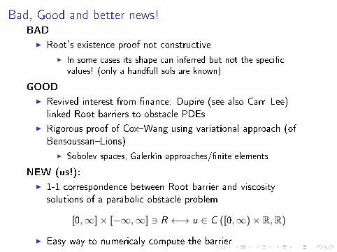
Bad, Good and better news!BAD
I Root's existence proof not constructive
I In some cases its shape can inferred but not the specicvalues! (only a handfull sols are known)
GOOD
I Revived interest from nance: Dupire (see also CarrLee)linked Root barriers to obstacle PDEs
I Rigorous proof of CoxWang using variational approach (ofBensoussanLions)
I Sobolev spaces, Galerkin approaches/nite elements
NEW (us!):
I 1-1 correspondence between Root barrier and viscositysolutions of a parabolic obstacle problem
[0,∞]× [−∞,∞] 3 R ←→ u ∈ C ([0,∞)× R,R)
I Easy way to numericaly compute the barrier
III.Root's barrier and Obstacle PDEs
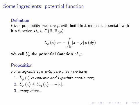
Some ingredients: potential function
DenitionGiven probability measure µ with nite rst moment, associate withit a function Uµ ∈ C (R,R≤0)
Uµ (x) := −ˆR|x − y |µ (dy)
We call Uµ the potential function of µ.
Proposition
For integrable v , µ with zero mean we have
1. Uµ (.) is concave and Lipschitz continuous,
2. Uµ (x) ≤ Uδ0 (x) = −|x |.3. many more...
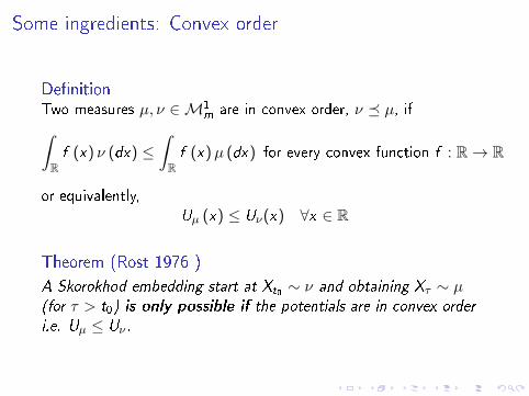
Some ingredients: Convex order
DenitionTwo measures µ, ν ∈M1
m are in convex order, ν µ, ifˆRf (x) ν (dx) ≤
ˆRf (x)µ (dx) for every convex function f : R→ R
or equivalently,Uµ (x) ≤ Uν(x) ∀x ∈ R
Theorem (Rost 1976 )
A Skorokhod embedding start at Xt0 ∼ ν and obtaining Xτ ∼ µ(for τ > t0) is only possible if the potentials are in convex order
i.e. Uµ ≤ Uν .
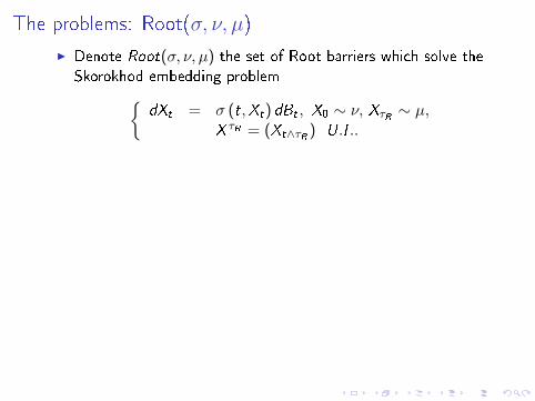
The problems: Root(σ, ν, µ)
I Denote Root(σ, ν, µ) the set of Root barriers which solve theSkorokhod embedding problem
dXt = σ (t,Xt) dBt , X0 ∼ ν, XτR ∼ µ,X τR = (Xt∧τR ) U.I ..
Proposition (GdR & H.Oberhauser 2012)
Let ν, µ ∈M2m , ν µ; σ > 0 and Lip & Lin. Grow.
dXt = σ (t,Xt) dBt , X0 ∼ ν,
where [X ]∞ =∞ or [lnX ]∞ =∞.
Then Root (σ, ν, µ) is not empty, i.e. there exists a Root barrier
s.t. X τR is UI and XτR ∼ µ.The barrier R is unique in the class of (ν, µ)-regular barriers, i.e.
R = R ∪ ([0,+∞]× x : Uν(x) = Uµ(x))
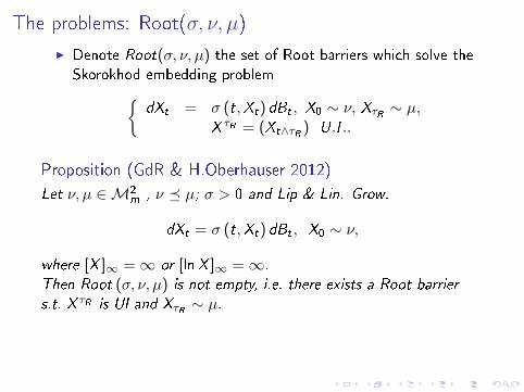
The problems: Root(σ, ν, µ)
I Denote Root(σ, ν, µ) the set of Root barriers which solve theSkorokhod embedding problem
dXt = σ (t,Xt) dBt , X0 ∼ ν, XτR ∼ µ,X τR = (Xt∧τR ) U.I ..
Proposition (GdR & H.Oberhauser 2012)
Let ν, µ ∈M2m , ν µ; σ > 0 and Lip & Lin. Grow.
dXt = σ (t,Xt) dBt , X0 ∼ ν,
where [X ]∞ =∞ or [lnX ]∞ =∞.
Then Root (σ, ν, µ) is not empty, i.e. there exists a Root barrier
s.t. X τR is UI and XτR ∼ µ.
The barrier R is unique in the class of (ν, µ)-regular barriers, i.e.
R = R ∪ ([0,+∞]× x : Uν(x) = Uµ(x))
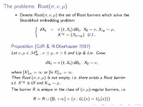
The problems: Root(σ, ν, µ)
I Denote Root(σ, ν, µ) the set of Root barriers which solve theSkorokhod embedding problem
dXt = σ (t,Xt) dBt , X0 ∼ ν, XτR ∼ µ,X τR = (Xt∧τR ) U.I ..
Proposition (GdR & H.Oberhauser 2012)
Let ν, µ ∈M2m , ν µ; σ > 0 and Lip & Lin. Grow.
dXt = σ (t,Xt) dBt , X0 ∼ ν,
where [X ]∞ =∞ or [lnX ]∞ =∞.
Then Root (σ, ν, µ) is not empty, i.e. there exists a Root barrier
s.t. X τR is UI and XτR ∼ µ.The barrier R is unique in the class of (ν, µ)-regular barriers, i.e.
R = R ∪ ([0,+∞]× x : Uν(x) = Uµ(x))
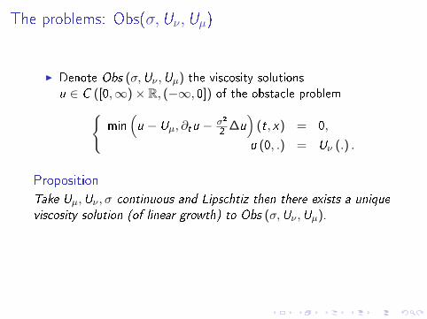
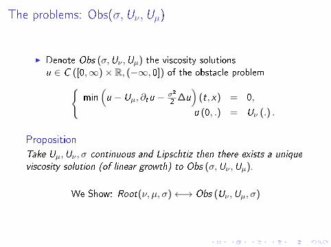
The problems: Obs(σ,Uν,Uµ)
I Denote Obs (σ,Uν ,Uµ) the viscosity solutionsu ∈ C ([0,∞)× R, (−∞, 0]) of the obstacle problem
min(u − Uµ, ∂tu − σ2
2∆u)
(t, x) = 0,
u (0, .) = Uν (.) .
Proposition
Take Uµ,Uν , σ continuous and Lipschtiz then there exists a unique
viscosity solution (of linear growth) to Obs (σ,Uν ,Uµ).
We Show: Root(ν, µ, σ)←→ Obs (Uν ,Uµ, σ)
From Barrier to PDE
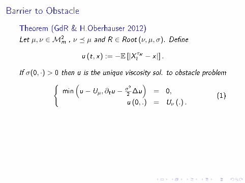
Barrier to Obstacle
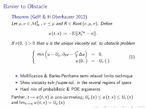
Theorem (GdR & H.Oberhauser 2012)
Let µ, ν ∈M2m , ν µ and R ∈ Root (ν, µ, σ). Dene
u (t, x) := −E [|X τRt − x |] .
If σ(0, ·) > 0 then u is the unique viscosity sol. to obstacle problemmin
(u − Uµ, ∂tu − σ2
2∆u)
= 0,
u (0, .) = Uν (.) .(1)
I Mollication & Barles-Perthame semi-relaxed limits technique
I Show viscosity sub-/super-sol. in the several regions of space
I Hard mix of probabilistic & PDE arguments
Further, t 7→ u (t, x) is non-increasing; Uµ (x) ≤ u (t, x) ≤ Uν (x)and limt→∞ u (t, x) = Uµ (x)
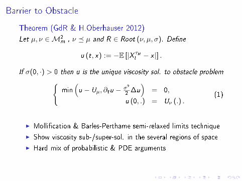
Barrier to Obstacle
Theorem (GdR & H.Oberhauser 2012)
Let µ, ν ∈M2m , ν µ and R ∈ Root (ν, µ, σ). Dene
u (t, x) := −E [|X τRt − x |] .
If σ(0, ·) > 0 then u is the unique viscosity sol. to obstacle problemmin
(u − Uµ, ∂tu − σ2
2∆u)
= 0,
u (0, .) = Uν (.) .(1)
I Mollication & Barles-Perthame semi-relaxed limits technique
I Show viscosity sub-/super-sol. in the several regions of space
I Hard mix of probabilistic & PDE arguments
Further, t 7→ u (t, x) is non-increasing; Uµ (x) ≤ u (t, x) ≤ Uν (x)and limt→∞ u (t, x) = Uµ (x)
From PDE to barrier
Obstacle to Barrier
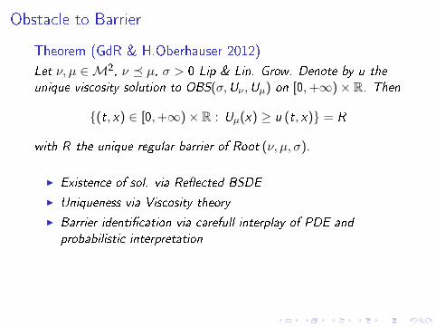
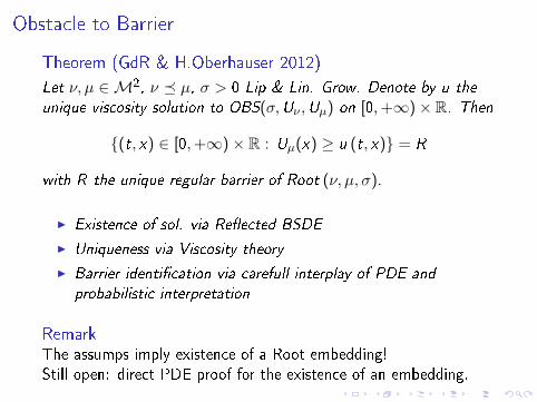
Theorem (GdR & H.Oberhauser 2012)
Let ν, µ ∈M2, ν µ, σ > 0 Lip & Lin. Grow. Denote by u the
unique viscosity solution to OBS(σ,Uν ,Uµ) on [0,+∞)× R. Then
(t, x) ∈ [0,+∞)× R : Uµ(x) ≥ u (t, x) = R
with R the unique regular barrier of Root (ν, µ, σ).
I Existence of sol. via Reected BSDE
I Uniqueness via Viscosity theory
I Barrier identication via carefull interplay of PDE and
probabilistic interpretation
RemarkThe assumps imply existence of a Root embedding!Still open: direct PDE proof for the existence of an embedding.
Obstacle to Barrier
Theorem (GdR & H.Oberhauser 2012)
Let ν, µ ∈M2, ν µ, σ > 0 Lip & Lin. Grow. Denote by u the
unique viscosity solution to OBS(σ,Uν ,Uµ) on [0,+∞)× R. Then
(t, x) ∈ [0,+∞)× R : Uµ(x) ≥ u (t, x) = R
with R the unique regular barrier of Root (ν, µ, σ).
I Existence of sol. via Reected BSDE
I Uniqueness via Viscosity theory
I Barrier identication via carefull interplay of PDE and
probabilistic interpretation
RemarkThe assumps imply existence of a Root embedding!Still open: direct PDE proof for the existence of an embedding.

For the numerics
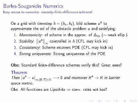
Barles-Souganidis NumericsEasy access to numerics: viscosity-nite-dierences schemes!
On a grid with timestep h = (hx , ht), bild scheme uh toapproximate the sol of the obstacle problem u and satisfying:
1. Monotonicity: of scheme in the approx. of ∆xx (∼ weak ellip.)
2. Stability:∥∥uh∥∥∞ controlled in h (CFL may kick in)
3. Consistency: Scheme recovers PDE (CFL may kick in)
4. Strong uniqueness: Strong uniqueness of the PDE
Obs: Standard nite-dierence schemes verify this! Great news!
TheoremThen
∣∣uh − u∣∣∞;[0,T ]×R −→ 0 and moreover Rh → R in barrier
space metric.
Obs: All functions are Lipschitz ⇒ conv. rates not bad!
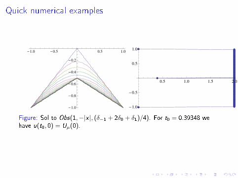
Quick numerical examples
-1.0 -0.5 0.5 1.0
-1.0
-0.8
-0.6
-0.4
-0.2
0.5 1.0 1.5 2.0
-1.0
-0.5
0.5
1.0
Figure: Sol to Obs(1,−|x |, (δ−1 + 2δ0 + δ1)/4). For t0 = 0.39348 wehave u(t0, 0) = Uµ(0).

Quick numerical examples
-1.0 -0.5 0.5 1.0
-1.0
-0.8
-0.6
-0.4
-0.2
0.5 1.0 1.5 2.0
-1.0
-0.5
0.5
1.0
Figure: Sol to Obs(1,−|x |, (δ−1 + 2δ0 + δ1)/4). For t0 = 0.39348 wehave u(t0, 0) = Uµ(0).
[1, 2, 5, 3, 4, 6]
A. M. G. Cox and J. Wang.Root's Barrier: Construction, Optimality and Applications toVariance Options.April 2011.
D. Hobson.The Skorokhod Embedding Problem and Model-IndependentBounds for Option Prices.In Paris-Princeton Lectures on Mathematical Finance 2010,volume 2003 of Lecture Notes in Mathematics, pages 267318.Springer Berlin / Heidelberg, 2011.
J. Obªój.On some aspects of Skorokhod embedding problem and itsapplications in mathematicas nance.Notes for the students of the 5th European summer school innancial mathematics, 2012.
D. H. Root.The existence of certain stopping times on Brownian motion.
Ann. Math. Statist., 40:715718, 1969.
H. Rost.The stopping distributions of a Markov Process.Invent. Math., 14:116, 1971.
A. V. Skorokhod.Studies in the theory of random processes.Translated from the Russian by Scripta Technica, Inc.Addison-Wesley Publishing Co., Inc., Reading, Mass., 1965.

THANK YOU FOR YOUR ATTENTION!


![Active Learning through Adversarial Exploration in ... · The typical NCE [5] approach in tasks such as word embeddings[18], order embeddings[27], and knowledge graph embeddings can](https://static.fdocuments.in/doc/165x107/5f1eea0ab232cb03ba65fafc/active-learning-through-adversarial-exploration-in-the-typical-nce-5-approach.jpg)