British Astronomical Association

VARIABLE STAR SECTION CIRCULAR

No 122, December 2004

Contents

ISSN 0267-9272

Office: Burlington House, Piccadilly, London, W1V 9AG

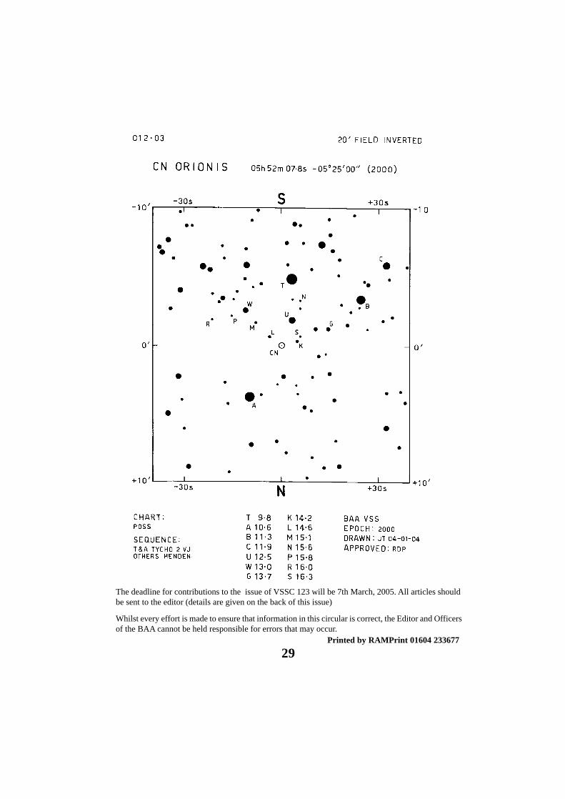
New Chart for CZ Orionis ..................................................... inside front coverFrom the Director ............................................................................................. 1An Unreconstructed Visual Observer - an Observer Profile ............................ 2Report on the Joint VS/I&I section CCD Photometry Meeting (Part 2) ......... 4An Exo-Planet Transit Search Programme ...................................................... 8Sunmmary of the Recent VSS Officers Meeting ........................................... 22Binocular Priority List ................................................................................... 24CCD Mentoring Scheme ................................................................................ 25Eclipsing Binary Predictions .......................................................................... 25New Chart for CN Orionis ..................................................... inside back cover

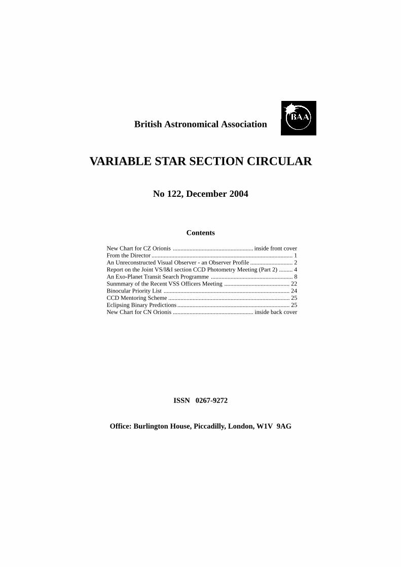
NEWLY ISSUED CHARTSJOHN TOONE

1

FROM THE DIRECTORROGER PICKARD

Dr Frank Bateson

Dr Frank Bateson, OBE, FRASNZ, retired at the beginning of December 2004 after 80 yearsof contributing to New Zealand and international Astronomy. I was therefore delighted whenJohn Toone announced that he would be attending the retirement ceremony, and would beable to personally deliver messages from the President, Tom Boles, and myself.

As a teenager in 1924, Frank Bateson published his first observation of variable stars, whilstin Sydney. In 1927 he joined the New Zealand Astronomical Society, now the Royal Astro-nomical Society of New Zealand, formed the Variable Star Section, and has been Directorever since. Under his Directorship it has grown to have an international reputation as theprincipal variable star organization in the Southern Hemisphere. Frank has been recognisedwith many awards from around the world for his services to astronomy.

His will be a hard act to follow. Congratulations, Frank on a most distinguished career.

VSS Meeting at Alston Hall

For those of you unable to attend this meeting, I regret to advise you that it was probably thebest yet! It was a truly excellent long weekend, thoroughly enjoyed by all. Make sure youdon’t miss the next one, although there are no plans at the moment, it is hoped that this will bein two or three years time, again at Alston Hall. But the meeting wouldn’t have been thesuccess it was without the excellent organisational skills of Denis Buczynski and his team,and the many excellent speakers, especially Mike Simonsen, who we worked quite hard.Thank you all. But even if you missed the meeting, you can start to read about it in the nextCircular thanks to Melvyn Taylor and Karen Holland who recorded details of all the talks.

No charge for charts

Following a recent discussion amongst the Officers, it has been agreed that charges for chartswill be abolished forthwith (although a large SAE will always be welcome, and will speed updelivery). Requests should still be made to the Chart or EB Secretarys as appropriate.

Reporting Observations

Although many observers now report their observations by email, there are still a numberwho report their observations on paper. Whilst we will always accept observations reportedin this way, it would be appreciated if those observers could consider reporting by email (ordisc) i.e. that they type up their own observations. This will relieve the small band of helperswho currently undertake this task, to concentrate on clearing the backlog of older observa-tions.

2

AN UNRECONSTRUCTED VISUAL OBSERVER, ANOBSERVER PROFILEMIKE GAINSFORD

I first became interested in astronomy at a very early age, late in the war, when we lived inLancashire (only seven miles from Alston Hall, where the 2004 BAA meeting was held).The first astronomy book I can recall, was Ball’s Romance of the Heavens. This was fol-lowed by other books from the library, culminating in Hutchinson’s Splendour of the Heav-ens, which was a major stimulus. I can remember my dad buying me George Philip’s Sign-post to the Stars. Along with the usual comics I took The Children’s Newspaper, which hadexcellent astronomical articles. At grammar school when I was 11 or 12, a teacher kindlyloaned me his 3” refractor. This was on a pillar and claw stand, and, although wobbly,enabled me to observe the summer objects I had only read about, by getting up at 3 in themorning. My parents weren’t too happy about this!

When we moved down to Leicester, for successive Christmas presents, I had a Broadhurstand Clarkson 2.25” refractor, and my own copy of Splendour of the Heavens. I spent manyhappy hours chasing Struve objects with the aid of the Cottam’s star maps in the back of thisbook. I now consider this somewhat of an achievement, and it was certainly a very soundgrounding in star-hopping. Have a look at these star maps sometime, if you are able. Whoneeds a GoTo facility? But at that time, I thought that variable stars could not possibly beinteresting.

National Service, studying, girls, marriage, and a family then meant that astronomy had totake a back seat for about ten years. But as a surveyor in the Royal Artillery, with Suezthreatening, two of us (both with astronomical interests) were speedily taught how to do starshots with a theodolite. We used Arcturus, and managed to pinpoint our position on Salis-bury Plain to within 3 miles.

My interest was rekindled in 1964 or 5 (possibly stimulated by the nearby Barwell meteoritefall). After much heart-searching as to whether it was right to do this with a young family tolook after, I approached the Midland Bank for a £200 loan (!), and got myself a Fullerscopes8.5” Newtonian. I joined the BAA (although I’d been buying their Handbook for years), andstarted to observe everything in sight, sending off the results to the various observing sec-tions. I also subscribed to The Astronomer, and sent my results there as well. I was on theBAA Council for two years in the early seventies.

In 1996, a number of moderately bright comets appeared, and I was so excited at my firstsight of one of these, my first ever comet (Kilston, I think), that I decided to submit estimatesof their brightness. How better to do this, but to practice on variable stars? But the practicebecame an obsession, and today I seldom observe anything else. To date, I have records ofaround 56,000 VS observations from 1966, but unfortunately, for eleven of these years Ihave no record. The real total may be more like 60,000.

But I’ll never make ‘the ton’. At 68, and going at my usual rate of 3000 in a good year, it willtake me at least until I’m 81! Age and creeping light-pollution will win, I’m afraid. I shouldn’thave wasted all those years on observing Mars, Jupiter, Saturn, meteors and various comets(only joking!).

3

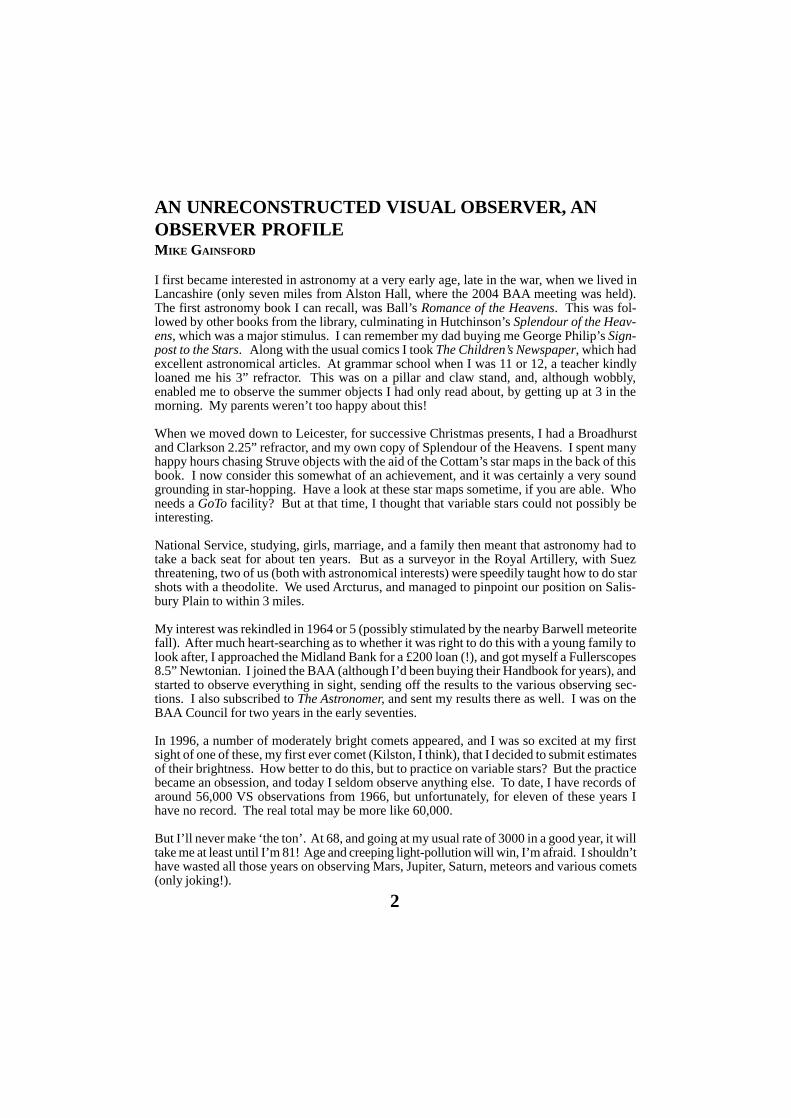
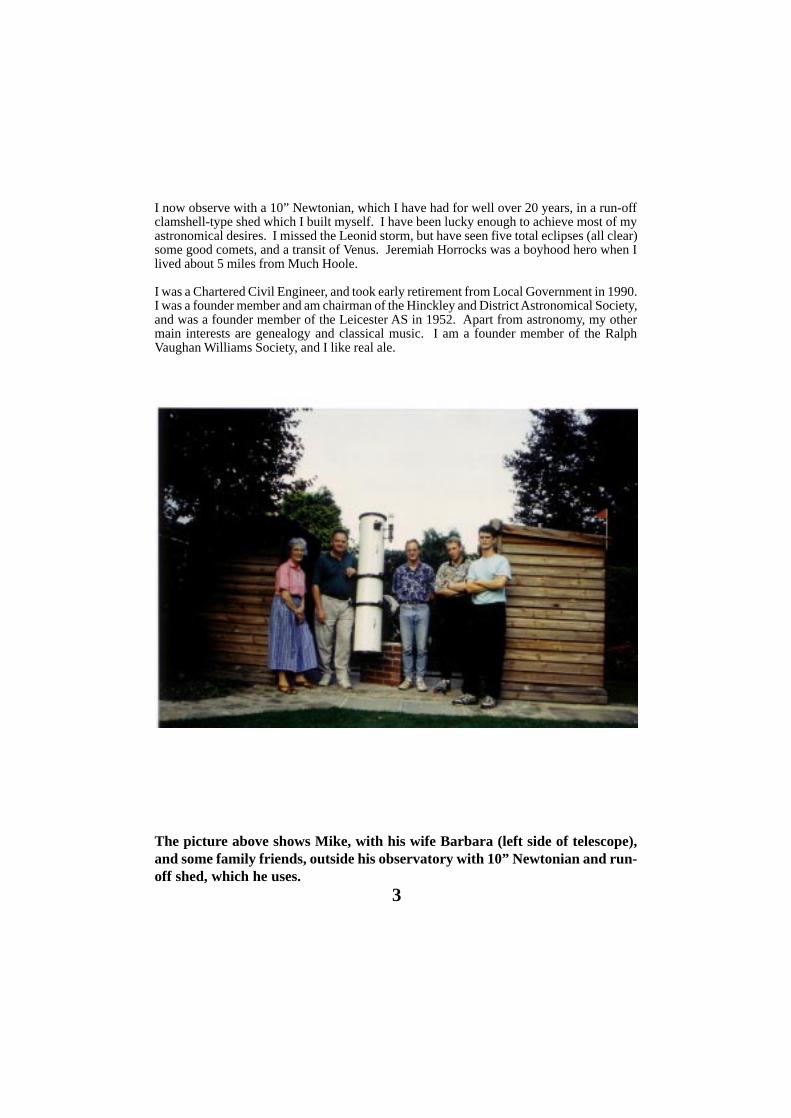
The picture above shows Mike, with his wife Barbara (left side of telescope),and some family friends, outside his observatory with 10” Newtonian and run-off shed, which he uses.

I now observe with a 10” Newtonian, which I have had for well over 20 years, in a run-offclamshell-type shed which I built myself. I have been lucky enough to achieve most of myastronomical desires. I missed the Leonid storm, but have seen five total eclipses (all clear)some good comets, and a transit of Venus. Jeremiah Horrocks was a boyhood hero when Ilived about 5 miles from Much Hoole.

I was a Chartered Civil Engineer, and took early retirement from Local Government in 1990.I was a founder member and am chairman of the Hinckley and District Astronomical Society,and was a founder member of the Leicester AS in 1952. Apart from astronomy, my othermain interests are genealogy and classical music. I am a founder member of the RalphVaughan Williams Society, and I like real ale.

4

REPORT ON THE JOINT VS/I&I SECTION CCD PHO-TOMETRY MEETING (PART 2)GARY POYNER AND KAREN HOLLAND

The Chairman for the Sunday morning session, Bob Marriott, introduced the first speaker ofthe day, who was David Boyd talking about A VS Section Excel spreadsheet to aid datareduction, a live demonstration in its use.

David introduced the MS Excel CCD data entry spreadsheet, which was available for CCDobservers, and which was an important tool for checking and standardising those observa-tions made with a CCD camera. Although it was now widely in use by UK observers, furtherdesign layouts would probably be available in the future.

David described the various entry fields in more detail, showing how they were colour-codedfor ease of use. These fields included in-depth information on the CCD (chip, noise etc),filter information, general observer information, information on the star under observationand the check star, sky brightness details and how the spreadsheet read data from AIP4WIN.

An example was shown with the Spreadsheet using data from KV Dra from personal obser-vations, and the procedures for loading data from AIP4WIN were described in some detail.The end result was then displayed as a light curve for the variable and check star. TheSummary sheet contained all of the relevant information used when reporting the informa-tion. David also showed how the output sheet read data from the spreadsheet, and convertedit to the AAVSO and BAAVSS reporting formats.

There were a few questions related to uploading data to the AAVSO, and the availability ofthe spreadsheet; it would be made available to download from the BAAVSS website. Nor-man Walker suggested that the JD date should be converted to HJD, and there was a discus-sion about this.

The Chairman thanked David for his presentation, and then introduced the Belgian CCDCBA observer Tonny Vanmunster to talk about A Demonstration of Peranso Software forTime Series Analysis of Lightcurves.

Tonny started by saying that his presentation on Peranso followed on nicely from David’soutline of his MS Excel spreadsheet, in that Peranso took data from other sources such asExcel, text files etc in a similar way. Peranso is, however, a complex and detailed dataanalysis program with many different functions. Tonny described Peranso in some detail,displaying the Observation, Period and Phase windows, which also included a HJD correc-tion. A light curve was displayed, in order to show how the properties of the graph could bealtered. Data from various observers could be entered using a variety of JD and magnitudeformats, including multiple observation sets, colour-coded for different observers.

Tonny then gave an example of the operation of Peranso using a large data set for Z UMafrom the AAVSO database, which included some 59,000 observations, in which a perioddetermination in a graphic and tabular form was shown. Following this, data on a Delta Scutistar was used to calculate multi-periods and perform a period accuracy check. Peranso alsochecked the analysis to determine whether the peaks displayed were real or false. A full help

5

facility and a very handy tutorial was included with the software. Norman Walker suggestedseveral improvements for future releases, but was very impressed with the software as itstood. Richard Miles asked whether Peranso could be used for Asteroid work, and Tonnyreplied that it was suitable for such analysis.

Next, Stan Waterman spoke about CCD photometry in Dense Star fields. This talk was verywell received, and many people wished to speak to Stan about his work during the day. As aresult of this, Stan has written up his talk as a separate article in this circular (starting on page8)

After the tea break, Arto Oksanen, who had travelled from Finland specifically for the meeting,gave an introduction to the CCD projects of Nyrola Observatory. This local society hadabout 250 members, of whom around 10% were observationally active. Arto showed picturesof some of the domes, and mentioned a new radio telescope project that the group wereinvolved in.

The group's main instruments were 16" and 10" Meade LX200 telescopes, together with anSBIG ST8XE and AO7 adaptive optics device. They had B,V and R filters which were usedon a slider. An Optec TCF-S focusser, Optec focal reducer, and a video camera with GPStime-setter for occulation work, all helped to make for a well-equipped observatory, whichwas completed by a permanent internet connection. All images collected were stored in FITsformat on a web server in real time, so that members could access the images collected inreal-time.

The first images started to be collected in 1999, initially practising taking images, and rapidlymoving on to more scientific work, including the monitoring of CVs, GRBs, blazar-monitoring,the collection of asteroid light-curves, the monitoring of Jovian moons (together with ArmaghUniversity) and exoplanet work.

The team appeared to be very dedicated. The eclipsing dwarf nova IY UMa had been observedthrough every single outburst since it was discovered; WZ Sge had been observed through itsrecent unexpectedly early outburst; they followed-up Sloan Digital Sky Survey CVs; GYCnc, an eclipsing dwarf nova of interest was a favorite target, as was the Delta Scuti variable(GSC3693) that they had discovered whilst observing OY Per when it was in outburst on oneoccasion.

Asteroid light curves were plotted for many asteroids, including the NEO Hermes 2003-10-18 which was originally discovered in 1911, and was lost, only to be rediscovered last year.

The group had spent a considerable amount of effort on exoplanet detection, collecting 900V-filtered images , each with a 10s integration time towards this project. They had found thatscintillation of the earth's atmosphere was a big problem in this field of study. In spite of thefact that the field of view was sufficiently small that they couldn't get the comparison star inthe image, they still managed to detect an exoplanet transit of the star HD209458, by averagingmany measurements together.

Blazars are a subclass of AGNs, that are billions of light years away. They are thought tohave one or more super-massive black holes at their centres. The group had been monitoring3C66A, at a rate of one image per night, and had also contributed to light curves of the blazar

6

S5 0716+71 during an international observing campaign.

The group were active supporters of the GRB network. They had a system up and runningwhich sent SMS alerts to members’ mobile telephones, so that they could look for afterglows.The first success that they had was in tracking the afterglow of GRB000926 on September28th, 2000. They followed this by producing multi-colour light curves of fading GRBafterglows, achieving the distinction of being the first amateurs to produce such a lightcurve.Arto also showed an interesting GRB afterglow lightcurve, which appeared to indicate thatthere was a delay in the red light, compared to the green light, but as Arto had been the onlyperson that was observing this at the time, it was difficult to confirm this unusual effect.

The society had plans to build an 80cm telescope that would be remotely-operable, and theyhad applied for EU funding to do this.

The next speaker of the day was James Weightman, who was talking about PhotometryExperiments with a Digital Camera. James described how he had been using a digitalcamera to take pretty pictures of the sky. He had decided to see if he could use it for photometry.His camera was a Canon EOS 300D DSLR CMOS sensor. It had an 85mm f1.2 lens. Heused it to obtain some images to try to create a light curve of a simple eclipsing binary, WUMa. He showed a range of images that he had taken using the camera, and the resultinglight curve. He felt that, whilst not of fantastic accuracy (the standard deviation on themeasurements appeared to be around 0.l magnitude), he felt that it had been a usefulexperiment.

Richard Miles commented that it was quite important, in this case, to ensure that the imagewas defocussed so that it occupied several pixels, as some of the CMOS sensor circuitryoccupied part of the chip’s area (the fill factor is not 100%). Defocussing to occupy manypixels reduces this effect.

After lunch David Boyd talked with a title of It's Surprising What you can Measure. Davidpresented his recent work on the CV DO Dra. This system was reported to be in outburstrecently, and so he followed the system over a night, and produced a light curve. He removeda low frequency variation which was not the orbital period, by calculating a running average,and this left him with a high frequency modulation. He used Tonny Vannmunster's Peransosoftware to do a period analysis on this remaining signal, and folded the light curve on thespin period of the system. This folding and binning process gave a much clearer indicationof the period of the system. He concluded that he had successfully detected the white dwarfspin period, and commented that, if this is the case, then it was the first ever direct detectionof the white dwarf spin period in the V band.

Gary pointed out that DO Dra showed interesting behaviour in that it occasionally rose inmagnitude up to around magnitude 13, which was not classed as a full-blown outburst, butwas only a partial outburst.

Next Norman Walker spoke with the title Amateur Photometry, a Strategy for Survival inthe Terabytes per day era of Professional Photometry. Norman wanted to focus on theareas where amateurs could still compete to do useful original work, in this day of robotictelescopes. He thought that if the professionals really could achieve the 1% accuracy thatthey hoped to, then this might reduce the numbers of projects available to amateurs, but hefelt that the 1% target might not necessarily be acheived. He had made measurements with a

7

precision of millimagnitude accuracy in the past, and felt that there were lots of potentialprojects, if amateurs were willing to work to achieve this level of accuarcy.

Norman showed a truly weird evolving light curve of Cygnus X1, that he had taken. Apparentlyno other B supergiant like Cygnus X1 had ever been investigated like this, and he felt thatthere was a lot of opportunity here.

Solar oscillations, at a level of 10-5 were too small a variation to monitor, and pulsars weretoo faint, but almost all the rest of the universe was up for grabs! Norman went on to describelots of the interesting projects available for amateurs, especially for CCD precision projects.He was particularly interested in non-radial oscillations that might exist in Mira-type stars.Non-radial pulsations exhibit equally-spaced frequencies, and Norman felt that there wassome evidence for this type of behaviour in Miras, which had not been properly investigatedto date.

Norman finished his talk by commenting that he felt that the cost of £250 per hour for the useof the Faulkes telescope was too expensive for most amateurs, particularly when you coulddo good work at home with currently available equipment.

The next speaker was John Saxton, who spoke about CCD Photometry at Lymm Observatory.Inspired by Don Kurtz's talk at Alston Hall last year, John had decided to monitor the whitedwarf ZZ PSc with his CCD camera. He showed his measurements which varied by about a10th of a magnitude. White dwarf oscillations have very short cycles, of the order of 4 perhour.

John then went on to describe his photometry software that he had developed based on TimNaylor's Optimal Extraction algorithm. This method used the Signal to Noise ratio in eachpixel to weight each pixel for the purpose of photometry. John had used his software toanalyse a series of stars in a field, and he had analysed the scatter to compare the results fromdoing the photometry using different methods (standard PSF and Optimal Extraction).

His trials seemed to indicate that optimal extraction gave a better standard deviation than asoft aperture; he compared the percentage scatter for both techniques. He did find that theoptimal extraction technique was the most troublesome for the faintest stars, and he developeda system by which he set the mask using the faintest star, and then used this for all other stars.The difficulty was that the mask was then not optimal for all the other stars. John's work wasvery interesting, and left us all with a lot to think about!

Richard Miles then spoke about the Calibration of Unfiltered Photometry. He started byshowing some examples of unusual spectra, in order to emphasize the range of targets thatwas available, which meant that filtering of CCD measurements was essential in almost allmeasurements.

In addition to the range of targets, CCD responses varied considerably too, and using a filteralso reduced the transmission. Most CCD users would choose filters that, when combinedwith their CCD responses, would ensure that their system approximated to either the Johnsonor the Hipparcos systems. Once a filter system was selected, M67 was a favorite target forproviding a selection of standard stars for the calculation of transformation coefficients.Richard had done a considerable amount of work to look at the transformation of Landolt V

8

standards to Hipparcos stars. He went on to say that he felt that his method of using Hipparcosred-blue pairs was a useful one. Although there was only one Hipparcos red-blue pair inM67, there were a great number of others available for use. Richard had examined theHipparcos catalogue, and had identified many red-blue pairs; they were all bright stars, whichmeant that the integration times for image acquisition would be short. Richard had acquiredthese images unfiltered, and had then calculated his transformation coefficients using these.He had used the unfiltered system applying a transformation to the results to obtain a Vmagnitude, and had used this method for different CCD cameras and felt that it worked verywell.

Richard went on to show how atmospheric extinction affected colours, and felt that it wasimportant to determine the dependence on colour of the extinction coefficient. He suggesteda number of targets for unfiltered photometry. He suggested that very faint supernovae, andasteroids with reflectance spectra, that show no absorption or emission lines, were suitabletargets. He thought that objects that were either very red or very blue in colour were notsuitable for this method.

Richard then went on to describe the Linearity Testing Kit that had been developed by JohnSaxton for testing CCD cameras. The kit was designed to reflect light on to the camera inthat same way that a flat field would, but the amount of light was altered by changing theLED’s duty cycle. Using this, it was possible to obtain some images, and selecting a nice flatpart of the flat field, the linearity measurements could be performed.

He showed the results for several CCD cameras including the Starlight MX916, which hadvery good linearity; the MX516, which was not quite as linear, but was acceptable for use ifrestricted to half its dynamic range; and the SXV H8 which had good linearity. Richardcommented that he had noticed other subtle effects that appeared to be taking place withmicrolensed chips, and he stressed that it was important to fully understand these systems inorder to perform good photometry with them.

After a brief discussion, the meeting was closed.

Editors note: Richard Miles has written up the aforementioned linearity measurements, andthey will be published in a future circular.

9

AN EXO-PLANET TRANSIT SEARCH PROGRAMSTAN WATERMAN

Introduction

This article is a modified version of the talk that I gave at the Pro-am CCD PhotometrySymposium on 15/16th May 2004 in Northampton. It covers more topics than the talk (I’veincluded those topics which I hope will be of particular interest or use to people), but in lessdetail, and is more of an overview of the highlights of the work to date.

Historical Note

I decided to attempt this project following a talk that was given to my local society in Octo-ber 2000, which included a mention of the transit of HD 209458. I thought to myself I coulddo that!, and that’s how all this work started. If I had known then, what I know now, I ratherdoubt I’d have started at all! Here is a sentence extracted from a recent email from TimBrown, who used to run STARE, and is a co-discoverer of the first, recent, and so far onlytransit discovery, TrES-1. I had originally supposed that I was going to do this whole projectmyself, put in a few months, find a bunch of planets, and show the world how easy it was.Well, it didn’t turn out that way.

Anyway, that’s now, not then, so I did make a start early in 2001, and although the first twoand a half years yielded no useful data, I learnt a lot. All the important elements of theanalysis programs were developed during that period, so it was a productive time from thatpoint of view. In the first observing season 2001/2002, I used a 12" reflector with a StarlightExpress MX camera, taking images in 30 contiguous areas of the sky in Cygnus on everyclear night, for as long as possible. Things have changed a lot since then; I now image one,much larger, area of Cygnus, and collect more data in 2 hours than I used to in the whole ofthat first season!

Equipment

For the 2003/2004 season, I used an Apogee AP16E camera with a Takahashi FS128 refrac-tor, and a focal reducer/ flattener to bring it to F/6; this gave me a 2.7 degree square field ofview. This season, I’ve been using a TMB130 F/6 refractor with a field flattener, and thesame CCD camera, which gives me the same field of view. Neither telescope is ideal for thejob: the Takahashi has a superior image quality over the field compared to the TMB (whichwas both a surprise and a disappointment), but it has very poor vignetting, which amounts toup to 50% in the corners of my field, a diameter of 52mm, compared to only 10% with theTMB.

Basic Concepts

The aim of the project remains to detect an extra solar planet by the transit method. What weare looking for is a Hot Jupiter similar to the HD209458 system (and indeed to TReS-1),which is likely to give a brightness dip of around 1-2% lasting in the region of 3 hours. Thatseems a pretty straightforward task on the face of it; the trouble is, there does not seem to bemany transits that are suitably aligned and timed for us, so one has to measure a lot of stars.

10

The other constraint is that you have to measure them for as long a continuous period aspossible, and for as many nights as are available. In addition, you need a high data rate toallow good noise-averaging within that approximate time frame of 3 hours. So all this meansthat you can’t go jumping around the sky to get lots of stars, you must stay in the same place.A large field of view is therefore essential, as is a rich target area. My chosen target area iscentred at 21 08 30/ 46 30 0. I imaged it from September to January last season, and frommid-August this year up to the current date. After quality filtering, I have 9522 good imagesfrom last season and (up to October ) 8,500 so far this season.

Data Flow

a) Images are collected in Fits format. A good October night can yield 9 hours or 600 images,sadly there are very few good nights in the UK!

b) The date and time is extracted, and they are converted to APL* files, dark-subtracted, flat-divided, and a global background is subtracted from the image. At this stage the brightnessof the image is assessed, and the background level across it measured. Cloud-affected orotherwise poor images are flagged at this stage.

c) The first step in the analysis is to find the brightest 6000 or so stars in each image, andmeasure their approximate brightness and accurate centroids.

d) Knowing the scale factor, these are then pattern-matched to a set from the same area of skyfrom the USNO B 1.0 catalogue. An iterative procedure is used to derive the picture coeffi-cients from the co-ordinates of the matching set, there is more detail on that below.

e) The co-ordinates (RA and Dec) from a pre-made starlist are converted to x and y pixelpositions for each image; the images are then probed at those points and a square of pixelscentred on each star is extracted. The samples vary from 23 pixels square for the brighteststars, to 13 pixels square for the faintest, with the star centroids in the centre pixel. Theapproximate magnitude range in the starlist is from magnitude 8 to 14; these are the 21,000brightest stars. This process reduces the amount of data that I need to store by about 10times: 6000 images take up 40Gb in APL format, but only about 4Gb if just the informationaround the target stars is retained. This is done image by image of course, but then thesamples are re-filed star by star, and added to the previous data for each star. The net resultis 21,000 files, one for each star (the ‘starbook’), and each with n pixel samples, where n isthe number of good images from the season. This makes a convenient database, which canbe stored and accessed from one hard drive, whilst containing all the information needed foreach star.

f) In addition to the above, each image is probed at 2401 (49 by 49) fixed RA and Dec co-ordinates, and samples of 91 pixels square are taken. These are added and averaged in sets of20 and 100 to provide a further database covering the whole image, rather then just the areaaround preselected stars. This is for the new object-finding program, see below. These formthe working databases for subsequent analysis.

Picture Coefficients

This is a vital link in the data reduction, so I provide a few more details here. There areobviously several ways of tracking a set of objects from images over a long period of time,

11

and one doesn’t need to use sky co-ordinates to do so. However, although more complicatedto set up, once it works, it enables one to have a fixed co-ordinate (J2000 equatorial RA andDec) for each object, which can be related to external catalogues. Also it allows one to imageany part of the sky, and then to get an automatic identification of all (well, most!) of theobjects in the image. The method I use is to pattern match from the brightest 6000 stars in theimage to a catalogue. That generally finds about 2,000 matches and a few wrong matches.The wrong ones can be removed by a first order fit. The rest are then sorted into 144 squaresacross the picture, and thinned to one per square. Generally some squares are empty at thisstage, so the program goes through sucessive approximations using second, third and fourthorder fits until it has a stable 4th order polynomial with a reference star in each square and alow rms error, of generally around 0.1 arcseconds. The reason for using this complex proce-dure is to take account of the moderately large field of view of the system (2.7degrees square).There is appreciable curvature of RA and Dec over that area, and there are also significantoptical system distortions (in terms of microns over the chip), so I found that a fourth orderpolynomial was necessary to get an rms error on the fit of the order of 0.1 arcseconds. Thereason for insisting that it fits all 144 reference stars, is that a higher order curve can rapidlydeviate if not constrained, particularly at the edges. Doing it this way, one can be certain thatthe picture will be probed wth an x/y error much less than a pixel, so a mis-identificationcan’t happen.

New Object Finding

I’ve been conscious for the last 12 months, that the system of probing the images only at apreset list of co-ordinates would mean that if, say, a nova was to pop up in the field of view,there is a 90% chance that it would not be noticed! So I’ve now got a simple but effectivesystem for avoiding that calamity, which uses the 100 and 20 average sets mentioned above.The reason for dividing each image up into lots of sub-squares is two-fold. There are minuteangle changes of the order of 0.01 degrees during a night, and even bigger errors from nightto night because I rotate the camera by 180 degrees at the E/W switchover, and the accuracyof repositioning is, at best, 0.1 degree. At the chip corners, 0.1 degree is 5 pixels, whichwould complicate the process of adding images and comparing the sums from night to night.

Using the sub-squares, with each one precisely centred at a particular RA and Dec, sucherrors are negligible. I had naively hoped that a simple correlation coefficient comparison ofeach of the 2401 averaged sample squares with ones from that night and previous ones wouldwork, but of course it doesn’t, beause a faint new object in a square containing some brightstars just wouldn’t be noticed. A much better method is to log an approximate brightness forall the objects in every square and look for changes. By averaging one hundred images, onecan see much deeper of course, and the program, in fact, finds and tracks 250,000 objects intotal, down to somewhere between magnitude 19 and 20. I run this program the day afterevery observing night, and it flags up, and presents a bitmap image, of anything which hasbrightened above mag 17, or has brightened by more than 2 magnitudes, or any new object.So far it has found between one and three new objects every time it has been run, but thesehave all so far been cosmic ray hits!

The Kodak Blue-Plus Pixels

There is no doubt that I bought the wrong camera for this project! The two-part nature of the‘E’ pixels led me into months of investigations to find the reason for the extra ‘noise’ and odd

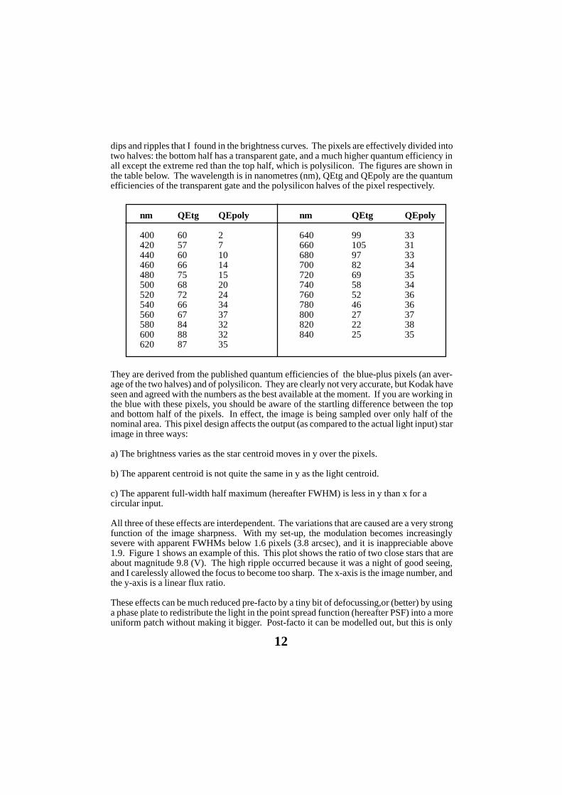
dips and ripples that I found in the brightness curves. The pixels are effectively divided intotwo halves: the bottom half has a transparent gate, and a much higher quantum efficiency inall except the extreme red than the top half, which is polysilicon. The figures are shown inthe table below. The wavelength is in nanometres (nm), QEtg and QEpoly are the quantumefficiencies of the transparent gate and the polysilicon halves of the pixel respectively.

nm QEtg QEpoly nm QEtg QEpoly

400 60 2 640 99 33420 57 7 660 105 31440 60 10 680 97 33460 66 14 700 82 34480 75 15 720 69 35500 68 20 740 58 34520 72 24 760 52 36540 66 34 780 46 36560 67 37 800 27 37580 84 32 820 22 38600 88 32 840 25 35620 87 35

They are derived from the published quantum efficiencies of the blue-plus pixels (an aver-age of the two halves) and of polysilicon. They are clearly not very accurate, but Kodak haveseen and agreed with the numbers as the best available at the moment. If you are working inthe blue with these pixels, you should be aware of the startling difference between the topand bottom half of the pixels. In effect, the image is being sampled over only half of thenominal area. This pixel design affects the output (as compared to the actual light input) starimage in three ways:

a) The brightness varies as the star centroid moves in y over the pixels.

b) The apparent centroid is not quite the same in y as the light centroid.

c) The apparent full-width half maximum (hereafter FWHM) is less in y than x for acircular input.

All three of these effects are interdependent. The variations that are caused are a very strongfunction of the image sharpness. With my set-up, the modulation becomes increasinglysevere with apparent FWHMs below 1.6 pixels (3.8 arcsec), and it is inappreciable above1.9. Figure 1 shows an example of this. This plot shows the ratio of two close stars that areabout magnitude 9.8 (V). The high ripple occurred because it was a night of good seeing,and I carelessly allowed the focus to become too sharp. The x-axis is the image number, andthe y-axis is a linear flux ratio.

These effects can be much reduced pre-facto by a tiny bit of defocussing,or (better) by usinga phase plate to redistribute the light in the point spread function (hereafter PSF) into a moreuniform patch without making it bigger. Post-facto it can be modelled out, but this is only

12

13

easy with good quality circularly-symmetric PSFs. Alternatively, one can use a better posi-tioned reference star. If the centroids of the two stars are separated in y by n+0.5 pixels (asin the cases in the figure), the modulation is at its maximum, whereas at integral separationsit almost disappears.

I now know that this is, in any case, not as serious a problem as I once thought, as the dipsearching routines are not seriously disturbed by these modulations.

Background Estimating

How to get the best possible estimate of the background level has been something I’ve spenta lot of time on over the years. I find that the errors that arise from this process are the mostimportant source of deviations in the faintest stars. For a star totalling 300 analogue todigital units (hereafter ADU), the faintest on my starlist, a random error of just one ADU canaffect the measurement by 6 or 7 %. If the effect were truly random, then it wouldn’t matter,because it could be reduced to a very reasonable 1% just by averaging about 40 images(about 36 minutes for me), but it almost certainly isn’t a random effect. The simplest methodto deal with this, is to find the mode of the pixels around the star, and then take an average ofthose within a few ADU of the mode. However, in Cygnus, this does not work reliablyenough, because of the high density of background stars. A better estimate can be found byaveraging a few hundred image samples from a star, so that the true background pixels can beidentified. This only needs to be done once, since the star centroid is always in the sameposition relative to those background pixels. They can then be used on each image to esti-mate the background.

That is still not ideal though, because with a limited number of pixels, the read-noise and thenoise in the background itself imposes a variation on the estimate. One has to either sacrificesome spatial variability or some temporal variability, to reduce the noise by averaging. I do

14

it spatially, by grouping the stars in 100 subsquares across the image, and then taking anaverage of the lowest half of the values for the stars in that box, except for those stars veryclose to a bright one; they have to be treated individually. How well the background isknown will determine the optimum strategy for forming brightness ratios. With good back-ground knowledge, it is generally better to use a selection of brighter stars to form ratios(with the same size circles or with a correction for FWHM). If the background is at alluncertain, then it is better to ratio stars of the same brightness as long as the stars are close toeach other and the same value of background is used for both.

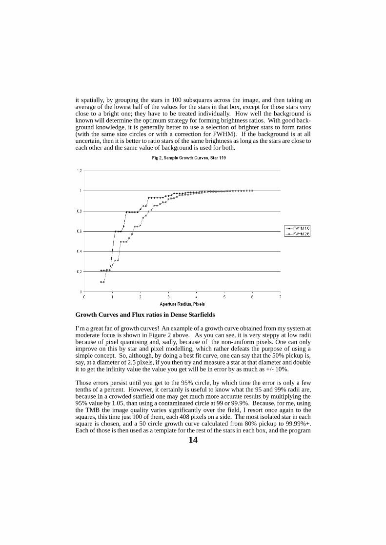
Growth Curves and Flux ratios in Dense Starfields

I’m a great fan of growth curves! An example of a growth curve obtained from my system atmoderate focus is shown in Figure 2 above. As you can see, it is very steppy at low radiibecause of pixel quantising and, sadly, because of the non-uniform pixels. One can onlyimprove on this by star and pixel modelling, which rather defeats the purpose of using asimple concept. So, although, by doing a best fit curve, one can say that the 50% pickup is,say, at a diameter of 2.5 pixels, if you then try and measure a star at that diameter and doubleit to get the infinity value the value you get will be in error by as much as +/- 10%.

Those errors persist until you get to the 95% circle, by which time the error is only a fewtenths of a percent. However, it certainly is useful to know what the 95 and 99% radii are,because in a crowded starfield one may get much more accurate results by multiplying the95% value by 1.05, than using a contaminated circle at 99 or 99.9%. Because, for me, usingthe TMB the image quality varies significantly over the field, I resort once again to thesquares, this time just 100 of them, each 408 pixels on a side. The most isolated star in eachsquare is chosen, and a 50 circle growth curve calculated from 80% pickup to 99.99%+.Each of those is then used as a template for the rest of the stars in each box, and the program

15

uses 95 or 99% circles as appropriate to the environs of that particular star. It’s very quick todo, and a star can be calculated for a whole season (10,000 ish samples) in a couple ofseconds.

For closely spaced stars a simple correction can be made for the influence of one on theother. Consider Fig 3 (above), the two circles represent the 95 or 99% circles for the stars(both the same). One star has a total true flux of a, the other of b, and these are the numbersthat we seek. The true amount of a in the overlap region is a1, similarly the overlap for b is

Figure 3, Closely-Spaced Stars need a Correction

b1. We can measure the apparent flux (just the aperture output) for the two stars, m1 and m2and also the combined total for both, T. Clearly we can write:

T=a+b .............................................................. 1m1=a+b1 .........................................................2m2=b+a1 ......................................................... 3a1/a=b1/b ........................................................ 4

So with these four equations we can find the 4 unknowns:

a=T(T -m2)/ 2T-(m1+m2)

and the rest follow.

Here is an example: the measured values are T=2000, m1=1500 and m2=1000. So, substi-tuting into the formula, a is 1333 and b is 667, which is a considerable difference from themeasured values, and substantially more accurate. A further small correction can be made,particularly if 95% circles are being used. Essentially all of that missing 5% is in an annulusa couple of pixels wide outside the 95% circle, so some of it is being collected by the otherstar, and this is pretty closely equal to the angles subtended or (arctan r/s)180 where r is themeasuring circle radius and s is the centroid separation. A typical value is about one fifth;

16

5%/5 is 1% so 1% of b needs to be subtracted from a and vice versa, and both of these needto be multiplied by 1.05 to get infinity values.Another simple correction can be used for faint stars close to much brighter ones. It isusually inaccurate to use 95 or 99% circles on very faint stars, and small circles are ill de-fined. I’ve found that, a better method is to use the ratio of the star and a close reference star,by using just the middle 9 pixels which generally covers about 70% of the total for me, withthe centroid somewhere in the middle pixel; this produces a result which is less noisy and lessprone to other errors compared to using circles.

If the faint star is close to a much brighter one, a not uncommon occurence in Cygnus, asimple correction can be applied that greatly improves the estimate for the faint star. For me,a typical 99% radius is 4 pixels. As an example, consider the case of a faint star just 5 pixelsaway from a star that is 5 magnitudes brighter, so that it is just outside the 99% circle. The 9pixels will then intercept (closely enough) one tenth of that 1% (or 10% of the faint star).This represents a substantial error and a large (but not uncommon) change in the PSF suchthat the 98% circle grows to where the 99% one was would double that. So simply taking offthese extra amounts contributed by the bright star, can greatly reduce the variability of thefaint star. By using tricks such as these I find it becomes possible to detect a 2% dip in eventhe faintest stars in the list.

Results so far: Noise and Precision

Averaging over a time interval of 30 minutes (33 images), the rms noise levels on a goodnight can vary from around 0.1% (S/N=1000) for stars of magnitude 8 to 9 up to 0.5% (S/N=200) for the faintest stars that I can sensibly measure at magnitude 13 to 14. This impliesa resolution, at best, of about 1millimagnitude for objects varying on timescales of not lessthan an hour. Fig 4 is a plot of a fast, low amplitude and irregular pulsator to illustrate thepoint. This is plotted for a running average of 30 data points, but is otherwise almost rawdata. The resolution is, of course, very different from my day to day accuracy, and I don’t yetknow what that is. This stability is of great importance for variable star work, but of almostno consequence as far as transit searching is concerned.

Results so far: Variable Stars

I haven’t yet produced an exhaustive listing of all the variable stars in ‘my’ small area ofCygnus, but of the 17,000 stars being monitored, more than a thousand vary in some way, andI suspect that number will grow to over 2,000. Most of the remaining ones will be uncoveredduring the transit searching, because the data has to be carefully cleaned and levelled for that.The stars that I have looked at, cover the expected range from long period, high amplitudered stars to low amplitude pulsators, down to periods of 50 minutes. I’m hoping to producea paper summarising the statistics in 6 to 12 months time.

Results so far: Transit Searching

As I write this (November 3rd), I’m within about a month of being able to search the databases for transit dips. The method has been tested, and the final figures show some simula-tion results. The detection method is very simple, and is just a matter of doing a runningcorrelation coefficient between the data, and a rectangular dip of the required length. I have

17

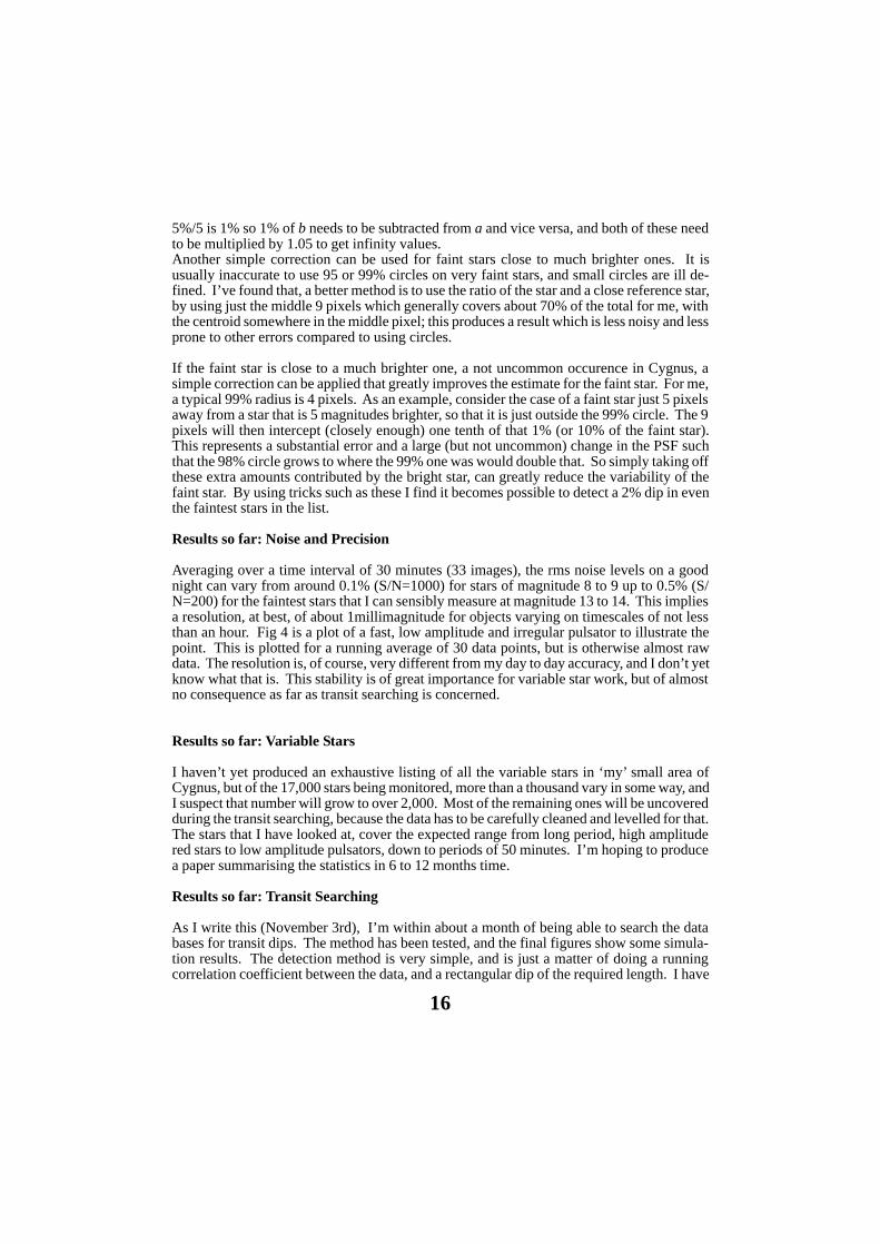
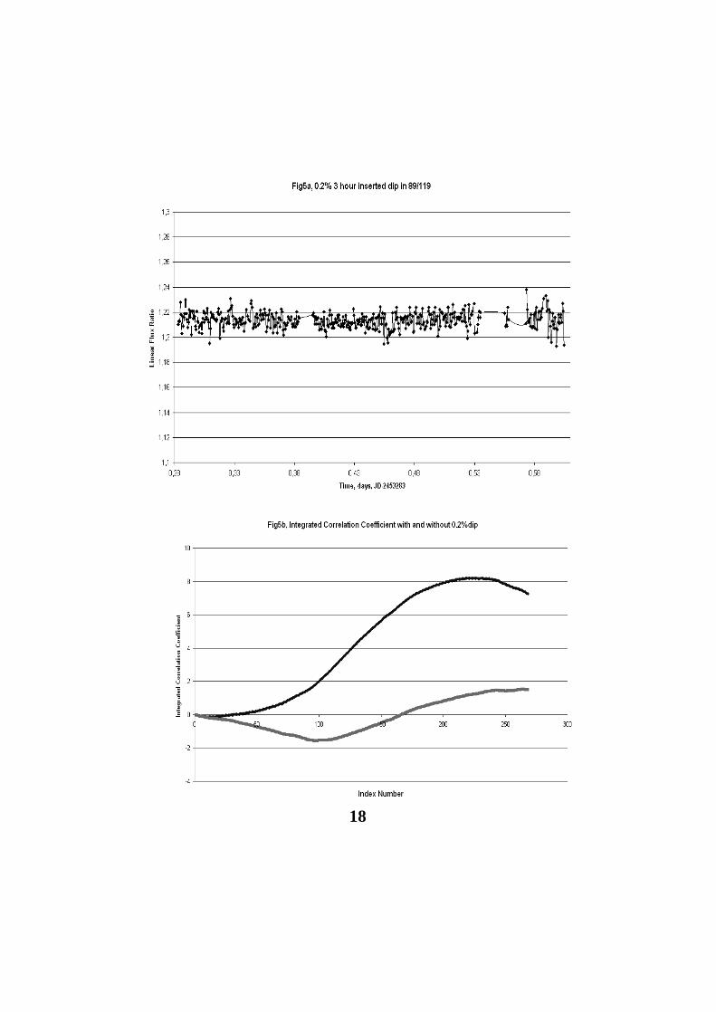
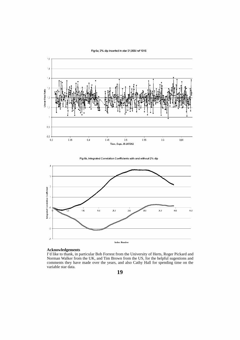
found the results to be more generally robust, if the correlator is followed by an integrator. Inprinciple it is all very simple: if the output from the integrator routine exceeds a threshold, adip has been found, so setting the threshold to minimise false alarms and maximise the chancesof a detection is the key to the process. On good data it works very well. In Fig 5a a 3 hour0.2% dip has been inserted into the brightness ratio data for a magnitude 9.8 (V) star. Theintegrator output for that input is shown in Fig 5b. The top curve is the output with the dipand the bottom curve the output without the dip. Clearly, if the threshold were set to anypositive value, a very clear detection would be achieved in this particular case, although thedip cannot be seen by eye in the data (though it can be with a 100pt running average). A morechallenging case is shown in Figs 6a and 6b. These are for one of the faintest stars in the fieldand are therefore much noisier; this time a 2% dip has been inserted. It so happens that thedata had a small positive movement in it, which is why the curve with no dip goes negative. Itcould equally well have gone positive though, so a threshold of at least 2.5 should be used.Even so, the detection is quite definite.

These results are extremely encouraging, in that they suggest that a 2% dip should be detect-able on a good proportion of the 17,000 stars being monitored. However, it is by no meansthat simple in reality, because a lot of the data is not as good as the examples I’ve shown andthe system still needs a lot of work to bring it to a state where the false alarm rate is accept-able. Even then, there will be a lot of false alarms from data artifacts to be examined. Addi-tionally, I expect that there will be astrophysical false alarms that I will need outside helpwith. I am told that these are likely to include, among other things, eclipsing binaries with abright companion which dilutes the dip and brings it down to the 1-2% level; eclipsing bina-ries with a line-of-sight companion; and eclipsing systems where one star is much brighterthan the other, producing a dip that is almost indistinguishable from a planet transit.

From the statistics behind the TrES-1 discovery, I know realistically that my chances of get-ting a confirmed transit out of the 2003/4 plus the 2004/5 data is only about 20%, but it’sgoing to be a lot of fun looking!

18

19

AcknowledgementsI’d like to thank, in particular Bob Forrest from the University of Herts, Roger Pickard andNorman Walker from the UK, and Tim Brown from the US, for the helpful sugestions andcomments they have made over the years, and also Cathy Hall for spending time on thevariable star data.

20

A SUMMARY OF THE MINUTES OF THE VSS OFFICERSMEETING, HELD ON MARCH 6TH 2004, AT SHOBDONMELVYN TAYLOR

Present: Roger Pickard, John Saxton, John Toone, Tony Markham, Gary Poyner, RichardMiles, Karen Holland

Apologies were received from Guy Hurst

The Database (Visual only)

John Saxton described how he was working to ensure that the database could be automati-cally-generated in the future; he was facilitating this by providing observers with appropri-ate software. If observers ran their observations through this software, it generated a checkedfile that was in the correct format for being accepted into the database. John usually ran thissoftware himself, but the beauty of asking the original observer to run the software, was thatthey could then correct the mistakes that the software would detect, which resulted in a fargreater degree of automation in the creation of the database.

There were a few minor “bugs” in the software, as with any new software, that John wasironing out. Once this had been completed, then John intended to proceed with an explana-tory article (see VS 119 p5).

Paper records

Roger commented that he was intending to collect all the outstanding paper records that stillneeded to be PC-entered from Crayford, for storing at Shobdon. There were possibly 4 filingcabinets of records left; he estimated that around 90% of all records were now in electronicformat. Currently, entering the data into PC format was being done by 6 people. Melvyncommented that 13 to 15 members were still reporting on paper.

It was noted that S Dunlop might have some years of data for AG Peg and CH Cyg, andMelvyn agreed to check on this. John Toone also thought that there might be some old SSCyg observations held by some members. Roger had been handed some observations byJ.Friends at the last BAA exhibition meeting, but had yet to check if they were already in thedatabase.

The Telescopic and Binocular Programmes

It was agreed that the status of telescopic stars that had no estimates in the database should bereviewed, and John Saxton agreed to check the database to identify which these were.

Melvyn was sure that several Miras and long period variables were under-observed. Binocu-lar variables had been categorised into three groups, and the priority list which appears ineach edition of the VSSC should be reviewed.

Norman Walker had offered to have a quick look to see if any possible periods could beidentified in the LB class of binocular variables, by performing a fourier analysis on the data.

21

The 2003 telescopic and binocular stars, for which observations had been reported on paper,still needed totalling for the Director’s report.

The Recurrent Objects Programme

Charts for this programme were being improved through the help of Henden and Simonsen.About 10 stars per year were added to the ROP. There were a few CCD observers of ROPstars, but most of the observers were visual observers, numbering around 4 at the start of theproject (ROP) in 1990, and numbering up to 20 to 30 at best.

Outbursts (numbering around 10 to 15 per year) were mainly reported by visual methods,with all UK estimates going to the database. There was a general rule that if a ROP object didnot have an observed outburst within 1 year of starting to be observed, then it was taken offthe list. Gary noted that the All Sky Survey was also monitoring recurrent novae, and othertypes of objects that were included on the ROP.

The Eclipsing Binary Programme

Tony reported that he was planning on reducing the eclipsing binary programme from 140stars to 95. The proposed transitional list appeared in VSSC 119 starting on page 11. Theeventual aim, was to try to reduce this further to around 70-80 stars.

The predicted times of minimum of programme objects continued to appear in the VSSC.The number of active observers was from around 8 to 10, and Tony was keen to encouragenew observers; his Winchester workshop article was to be in the August JBAA, which wouldbe appearing at about the right time for potential new observers to take on long runs ofestimates over the winter. The forthcoming Eta Gem eclipse minimum was discussed, with asubsequent article in VS120 page 17.

The “New” VS Programme

This programme consisted of 20 of Mike Collin’s discoveries, and were mainly being fol-lowed by Hazel McGee, Chris Jones, Graham Salmon and Richard Hunt.

Charts and sequences

The International Chart working group, of which John had been a member, appeared to have“fizzled-out”. John mentioned that assistance from Henden and Simonsen had been veryuseful in the amendment of comparison star sequences, especially for some ROP objects.John had been offered some assistance with drawing charts, and had been working with up tothree assistants on charts.

A request was made for all good charts to be put on the web pages for ease of access. DavidGriffin had scanned many charts, and so this should be possible. The chart catalogue nowhad all telescopic and binocular variables in constellation order.

The Faulkes Telescope

Roger wondered if it might be possible to use the Faulkes Telescope to check comparison

22

star sequences. It was agreed that a list should be drawn up to include all stars for whichsequences needed measuring. This should include RA and Dec for each star, treating ROPstars as priority, then miras and long period variables, followed by semi-regulars. Richardsuggested that the TASS sky survey could also be used for sequence-checking, and that itwas accessible via the Web. This had the advantage of providing V-I colour magnitudes, andmight therefore help in the selection of comparison stars of a similar colour to the variable, aswell as checking for the possibility of intrinsic variability of comparison stars.

Circulars

Karen reported that over the 8 years that she had been producing the circular, the number ofsubscribers had increased from less than 150 to 170. The next issue was to be a bumper sizeissue again. Karen commented that there was a general shortage of articles, and requestedreadable, news articles, observer profiles along with any other contributions. Six subscribershad converted to PDF subscriptions, and this appeared to be an attractive way of accessingthe circulars, leaving a few more paper copies spare for selling at meetings, or offering topotential new members. Several CDs of VSSCs in PDF format had been sold.

Pro-Am Liason Committee

Roger told the group that whilst this group had served a useful purpose during its existence,it had now wound-up.

CCD Photometry and the CCD Database

The CCD target list was now on the web site, and for ease of display at meetings the list hadbeen reproduced as a poster. The list contains four different categories of project: 1) basicphotometry, 2) time-series photometry, 3) approximate differential photometry, 4) precisionphotometry. Some objects have CCD charts to ease measurement of the objects, but it wasnoted that more were required. It was agreed that, except where there was a danger of mis-identification of a star, the CCD sequence would not need to be reproduced in chart form, butcould take the form of a list including the relevant information.

Richard said that he was working to finalise a simplified form of the PEP template in readi-ness for the May CCD Workshop. The CCD committee currently consisted of David Boyd,Richard Miles, Roger Pickard, Karen Holland and Andy Wilson.

CCD Photometry Workshop

Karen reported that the arrangements for this two-day meeting, to be held in Northampton,were well in hand. Karen was looking for suitable overnight accommodation, and noted thatthe meeting might be a good time to launch a CCD mentoring scheme.

The workshop programme currently had David Boyd, John Saxton, Roger Pickard, RichardMiles, Karen Holland and Nick James contributing. Richard said that he would email detailsof the Symposium to known international groups e.g. the Yahoo e-Group on CCD-Astrometry-Photometry. Melvyn suggested that members of the IOTA ESOP group might also be inter-ested.

23

Section meeting at Alston Hall

Another two day VSS meeting was planned at Alston Hall for 2004, over the weekend ofOctober 22 to 24. It had been decided that the meeting would start on the Friday afternoon,and would finish at lunchtime on the Sunday in the hope that travel would be easier with thisarrangement.

Professor Don Kurtz was already booked, and it was hoped that Mike Simonsen, BruceSumner and Professor Tom Harquist (Leeds University) might also attend.

Observing Guide

Roger reported that this was an A5 sized 64 page booklet, containing general informationregarding observing, and including some charts for various telescopic, binocular and eclips-ing binary stars. This was to include some charts on an accompanying CD, but plans for thishad now been abandoned. Don Miles had been contacted with the material and art work forthe production of this guide, but progress to date had been slow.

Web Site

Roger reported that the VSS Web site now contained notice of the May CCD Symposium.The chart cataloging had not been a success. Since Peter Moreton’s resignation, it wasnecessary to find a new webmaster, and David Grover, David Griffin and John Fairweatherwere all possible replacements.

UK alert group

This had been started on January 17th, 2004, and there were now a total of 33 members/subscribers; 64 messages had been transferred at the date of this meeting. Gary noted thatthere were several overseas subscribers, including VSNET members.

Mentoring Scheme

Karen noted that after a relatively slow start there were now 5 visual mentees, 3 CCD menteesand 19 mentors. Karen was hoping to launch the CCD mentoring scheme at the May 16/17event.

Posters

Karen asked if anyone had any ideas for possible themes for posters in size A3 to A1. A2sizes were best suited to our display boards, but small-sized A4 to A3 posters were the opti-mum size for being laminated.

AOB

Karen wondered if the increasing number of CCD photometry specific articles that werebeing contributed for the VSSC, should be presented in a separate occasional CCD specificpublication, but it was agreed that they should continue to be published in the existing VSSC.

24

Variable Range Type PeriodChart

AQ And 8.0-8.9 SRC 346d 82/08/16EG And 7.1-7.8 ZA 072.01V Aql 6.6-8.4 SRB 353d 026.03UU Aur 5.1-6.8 SRB 234d 230.01.AB Aur 7.2-8.4 INA 83/10/01V Boo 7-12 SRA 258d 037.01RW Boo 6.4-7.9 SRB 209d 104.01RX Boo 6.9-9.1 SRB 160d 219.01ST Cam 6.0-8.0 SRB 300d? 111.01XX Cam 7.3-9.7? RCB? 068.01X Cnc 5.6-7.5 SRB 195d 231.01RS Cnc 5.1-7.0 SRC 120d? 84/04/12V CVn 6.5-8.6 SRA 192d 214.01WZ Cas 6.9-8.5 SRB 186d 82/08/16V465 Cas 6.2-7.2 SRB 60d 233.01γ γ γ γ γ Cas 1.6-3.0 GC 064.01rho Cas 4.1-6.2 SRD 320d 064.01W Cep 7.0-9.2 SRC 83/10/01AR Cep 7.0-7.9 SRB 85/05/06mu Cep 3.4-5.1 SRC 730d 112.01ΟΟΟΟΟ Cet 2.0-10.1 M 332d 039.02R CrB 5.7-14.8 RCB 041.02W Cyg 5.0-7.6 SRB 131d 062.1AF Cyg 6.4-8.4 SRB 92d 232.01CH Cyg 5.6-10.0ZA+SR 089.02U Del 5.6-7.5 SRB 110d? 228.01EU Del 5.8-6.9 SRB 60d? 228.01TX Dra 6.8-8.3 SRB 78d? 106.01

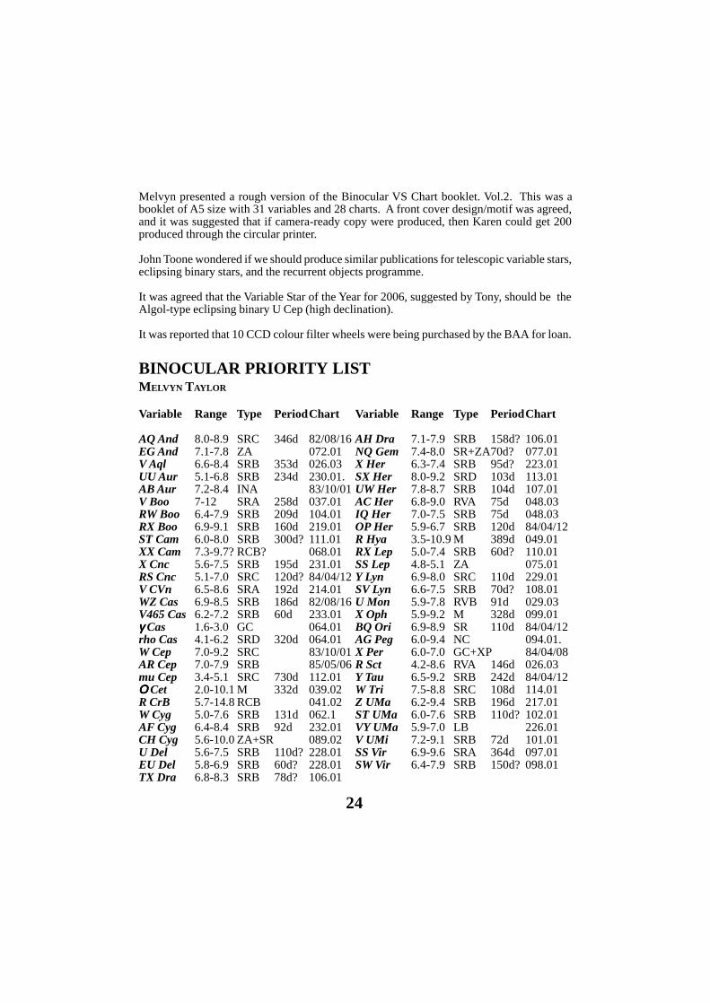
BINOCULAR PRIORITY LISTMELVYN TAYLOR

Variable Range Type PeriodChart

AH Dra 7.1-7.9 SRB 158d? 106.01NQ Gem 7.4-8.0 SR+ZA70d? 077.01X Her 6.3-7.4 SRB 95d? 223.01SX Her 8.0-9.2 SRD 103d 113.01UW Her 7.8-8.7 SRB 104d 107.01AC Her 6.8-9.0 RVA 75d 048.03IQ Her 7.0-7.5 SRB 75d 048.03OP Her 5.9-6.7 SRB 120d 84/04/12R Hya 3.5-10.9 M 389d 049.01RX Lep 5.0-7.4 SRB 60d? 110.01SS Lep 4.8-5.1 ZA 075.01Y Lyn 6.9-8.0 SRC 110d 229.01SV Lyn 6.6-7.5 SRB 70d? 108.01U Mon 5.9-7.8 RVB 91d 029.03X Oph 5.9-9.2 M 328d 099.01BQ Ori 6.9-8.9 SR 110d 84/04/12AG Peg 6.0-9.4 NC 094.01.X Per 6.0-7.0 GC+XP 84/04/08R Sct 4.2-8.6 RVA 146d 026.03Y Tau 6.5-9.2 SRB 242d 84/04/12W Tri 7.5-8.8 SRC 108d 114.01Z UMa 6.2-9.4 SRB 196d 217.01ST UMa 6.0-7.6 SRB 110d? 102.01VY UMa 5.9-7.0 LB 226.01V UMi 7.2-9.1 SRB 72d 101.01SS Vir 6.9-9.6 SRA 364d 097.01SW Vir 6.4-7.9 SRB 150d? 098.01

Melvyn presented a rough version of the Binocular VS Chart booklet. Vol.2. This was abooklet of A5 size with 31 variables and 28 charts. A front cover design/motif was agreed,and it was suggested that if camera-ready copy were produced, then Karen could get 200produced through the circular printer.

John Toone wondered if we should produce similar publications for telescopic variable stars,eclipsing binary stars, and the recurrent objects programme.

It was agreed that the Variable Star of the Year for 2006, suggested by Tony, should be theAlgol-type eclipsing binary U Cep (high declination).

It was reported that 10 CCD colour filter wheels were being purchased by the BAA for loan.

25

ECLIPSING BINARY PREDICTIONSTONY MARKHAM

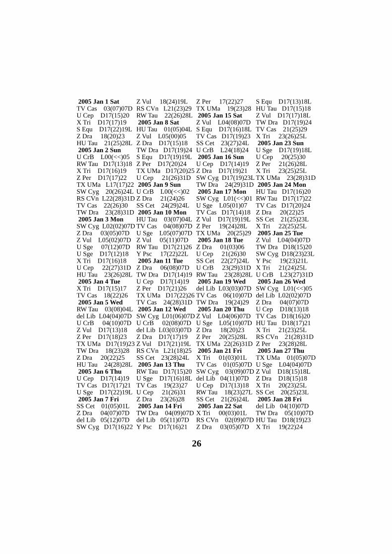
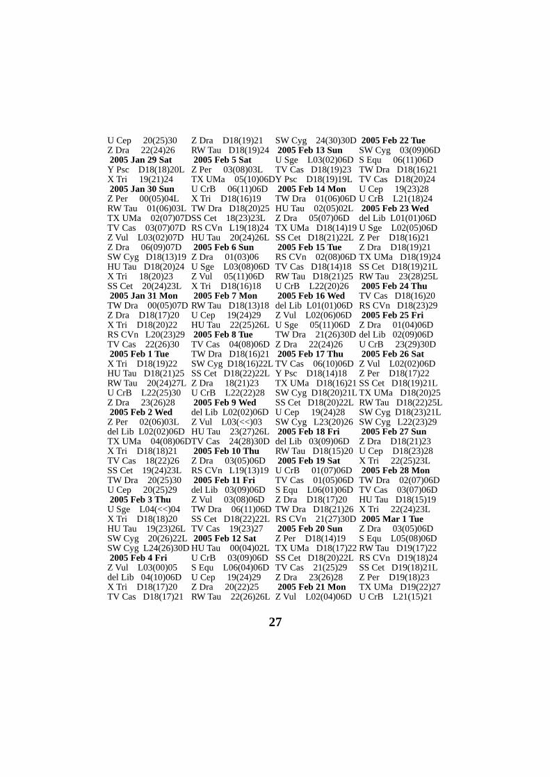
The following predictions, based on the latest Krakow elements, should be usable for observers through-out the British Isles. The times of mid-eclipse appear in parentheses, with the start and end times ofvisibility on either side. The times are hours UT, with a value greater than 24 indicating atime after midnight. D indicates that the eclipse starts/end in daylight, L indicates low alti-tude at the start/end of the visibility and << indicates that mid eclipse occurred on an earlierdate.

Thus, for example, on Jan 8, TW Dra D17(19)24 indicates that TW Dra will be in mideclipse at approx 19h UT. The eclipse will be observable between approx 17h UT and mid-night UT, with the start of the eclipse having occurred during daylight. Please contact the EBsecretary if you require any further explanation of the format.

The variables covered by these predictions are :

RS CVn 7.9-9.1V Z Dra 10.8-14.1p U Sge 6.45-9.28VTV Cas 7.2-8.2V TW Dra 8.0-10.5v RW Tau 7.98-11.59VU Cep 6.75-9.24V S Equ 8.0-10.08V HU Tau 5.92-6.70VSS Cet 9.4-13.0v delta Lib 4.9-5.9V X Tri 8.88-11.27VU CrB 7.7-8.8V Z Per 9.7-12.4p TX UMa 7.06-8.80VSW Cyg 9.24-11.83 VY Psc 9.44-12.23V Z Vul 7.25-8.90V

Note that predictions for RZ Cas, Beta Per and Lambda Tau can be found in the BAAHandbook.

Several long period eclipsing variables have eclipses due during this interval. Theseinclude BL Tel (mid eclipse Jan 08), BM Cas (Jan 20), mu Sgr (Feb 10) and W Cru (Mar09). For further details, see VSSC 114.

THE VS CCD MENTORING SCHEMEKAREN HOLLAND

The Variable Star Mentoring Scheme was set up a couple of years ago specifically to assistnew visual observers, or observers who were new to the field of Variable Star Observing.Following the success of this scheme, and after a number of requests, a CCD Mentoringscheme has now been set up. The aim is to provide newcomers to CCD photometry, a mentorto whom they can turn for guidance or advice, whilst they learn the techniques essential togood photometry. As much, or as little, assistance as is required can be offered. As with theVisual mentoring scheme, it is thought that some CCD observers will require a mentor for ashort time, to provide confirmation of their already good methods, whilst others may requireguidance for a longer period. If you feel a CCD mentor would be useful to you, pleasecontact Karen Holland (details on the back cover) to be allocated a mentor.

26

2005 Jan 1 SatTV Cas 03(07)07DU Cep D17(15)20X Tri D17(17)19S Equ D17(22)19LZ Dra 18(20)23HU Tau 21(25)28L 2005 Jan 2 SunU CrB L00(<<)05RW Tau D17(13)18X Tri D17(16)19Z Per D17(17)22TX UMa L17(17)22SW Cyg 20(26)24LRS CVn L22(28)31DTV Cas 22(26)30TW Dra 23(28)31D 2005 Jan 3 MonSW Cyg L02(02)07DZ Dra 03(05)07DZ Vul L05(02)07DU Sge 07(12)07DU Sge D17(12)18X Tri D17(16)18U Cep 22(27)31DHU Tau 23(26)28L 2005 Jan 4 TueX Tri D17(15)17TV Cas 18(22)26 2005 Jan 5 WedRW Tau 03(08)04Ldel Lib L04(04)07DU CrB 04(10)07DZ Vul D17(13)18Z Per D17(18)23TX UMa D17(19)23TW Dra 18(23)28Z Dra 20(22)25HU Tau 24(28)28L 2005 Jan 6 ThuU Cep D17(14)19TV Cas D17(17)21U Sge D17(22)19L 2005 Jan 7 FriSS Cet 01(05)01LZ Dra 04(07)07Ddel Lib 05(12)07DSW Cyg D17(16)22

Z Vul 18(24)19LRS CVn L21(23)29RW Tau 22(26)28L 2005 Jan 8 SatHU Tau 01(05)04LZ Vul L05(00)05Z Dra D17(15)18TW Dra D17(19)24S Equ D17(19)19LZ Per D17(20)24TX UMa D17(20)25U Cep 21(26)31D 2005 Jan 9 SunU CrB L00(<<)02Z Dra 21(24)26SS Cet 24(29)24L 2005 Jan 10 MonHU Tau 03(07)04LTV Cas 04(08)07DU Sge L05(07)07DZ Vul 05(11)07DRW Tau D17(21)26Y Psc 17(22)22L 2005 Jan 11 TueZ Dra 06(08)07DTW Dra D17(14)19U Cep D17(14)19Z Per D17(21)26TX UMa D17(22)26TV Cas 24(28)31D 2005 Jan 12 WedSW Cyg L01(06)07DU CrB 02(08)07Ddel Lib L03(03)07DZ Dra D17(17)19Z Vul D17(21)19LRS CVn L21(18)25SS Cet 23(28)24L 2005 Jan 13 ThuRW Tau D17(15)20U Sge D17(16)18LTV Cas 19(23)27U Cep 21(26)31Z Dra 23(26)28 2005 Jan 14 FriTW Dra 04(09)07Ddel Lib 05(11)07DY Psc D17(16)21

Z Per 17(22)27TX UMa 19(23)28 2005 Jan 15 SatZ Vul L04(08)07DS Equ D17(16)18LTV Cas D17(19)23SS Cet 23(27)24LU CrB L24(18)24 2005 Jan 16 SunU Cep D17(14)19Z Dra D17(19)21SW Cyg D17(19)23LTW Dra 24(29)31D 2005 Jan 17 MonSW Cyg L01(<<)01U Sge L05(01)07TV Cas D17(14)18Z Vul D17(19)19LZ Per 19(24)28LTX UMa 20(25)29 2005 Jan 18 TueZ Dra 01(03)06U Cep 21(26)30SS Cet 22(27)24LU CrB 23(29)31DRW Tau 23(28)28L 2005 Jan 19 Weddel Lib L03(03)07DTV Cas 06(10)07DTW Dra 19(24)29 2005 Jan 20 ThuZ Vul L04(06)07DU Sge L05(10)07DZ Dra 18(20)23Z Per 20(25)28LTX UMa 22(26)31D 2005 Jan 21 FriX Tri 01(03)01LTV Cas 01(05)07DSW Cyg 03(09)07Ddel Lib 04(11)07DU Cep D17(13)18RW Tau 18(23)27LSS Cet 21(26)24L 2005 Jan 22 SatX Tri 00(03)01LRS CVn 02(09)07DZ Dra 03(05)07D

S Equ D17(13)18LHU Tau D17(15)18Z Vul D17(17)18LTW Dra D17(19)24TV Cas 21(25)29X Tri 23(26)25L 2005 Jan 23 SunU Sge D17(19)18LU Cep 20(25)30Z Per 21(26)28LX Tri 23(25)25LTX UMa 23(28)31D 2005 Jan 24 MonHU Tau D17(16)20RW Tau D17(17)22TV Cas D17(20)24Z Dra 20(22)25SS Cet 21(25)23LX Tri 22(25)25L 2005 Jan 25 TueZ Vul L04(04)07DTW Dra D18(15)20SW Cyg D18(23)23LY Psc 19(23)21LX Tri 21(24)25LU CrB L23(27)31D 2005 Jan 26 WedSW Cyg L01(<<)05del Lib L02(02)07DZ Dra 04(07)07DU Cep D18(13)18TV Cas D18(16)20HU Tau D18(17)21X Tri 21(23)25LRS CVn 21(28)31DZ Per 23(28)28L 2005 Jan 27 ThuTX UMa 01(05)07DU Sge L04(04)07DZ Vul D18(15)18LZ Dra D18(15)18X Tri 20(23)25LSS Cet 20(25)23L 2005 Jan 28 Fridel Lib 04(10)07DTW Dra 05(10)07DHU Tau D18(19)23X Tri 19(22)24

27

U Cep 20(25)30Z Dra 22(24)26 2005 Jan 29 SatY Psc D18(18)20LX Tri 19(21)24 2005 Jan 30 SunZ Per 00(05)04LRW Tau 01(06)03LTX UMa 02(07)07DTV Cas 03(07)07DZ Vul L03(02)07DZ Dra 06(09)07DSW Cyg D18(13)19HU Tau D18(20)24X Tri 18(20)23SS Cet 20(24)23L 2005 Jan 31 MonTW Dra 00(05)07DZ Dra D18(17)20X Tri D18(20)22RS CVn L20(23)29TV Cas 22(26)30 2005 Feb 1 TueX Tri D18(19)22HU Tau D18(21)25RW Tau 20(24)27LU CrB L22(25)30Z Dra 23(26)28 2005 Feb 2 WedZ Per 02(06)03Ldel Lib L02(02)06DTX UMa 04(08)06DX Tri D18(18)21TV Cas 18(22)26SS Cet 19(24)23LTW Dra 20(25)30U Cep 20(25)29 2005 Feb 3 ThuU Sge L04(<<)04X Tri D18(18)20HU Tau 19(23)26LSW Cyg 20(26)22LSW Cyg L24(26)30D 2005 Feb 4 FriZ Vul L03(00)05del Lib 04(10)06DX Tri D18(17)20TV Cas D18(17)21

Z Dra D18(19)21RW Tau D18(19)24 2005 Feb 5 SatZ Per 03(08)03LTX UMa 05(10)06DU CrB 06(11)06DX Tri D18(16)19TW Dra D18(20)25SS Cet 18(23)23LRS CVn L19(18)24HU Tau 20(24)26L 2005 Feb 6 SunZ Dra 01(03)06U Sge L03(08)06DZ Vul 05(11)06DX Tri D18(16)18 2005 Feb 7 MonRW Tau D18(13)18U Cep 19(24)29HU Tau 22(25)26L 2005 Feb 8 TueTV Cas 04(08)06DTW Dra D18(16)21SW Cyg D18(16)22LSS Cet D18(22)22LZ Dra 18(21)23U CrB L22(22)28 2005 Feb 9 Weddel Lib L02(02)06DZ Vul L03(<<)03HU Tau 23(27)26LTV Cas 24(28)30D 2005 Feb 10 ThuZ Dra 03(05)06DRS CVn L19(13)19 2005 Feb 11 Fridel Lib 03(09)06DZ Vul 03(08)06DTW Dra 06(11)06DSS Cet D18(22)22LTV Cas 19(23)27 2005 Feb 12 SatHU Tau 00(04)02LU CrB 03(09)06DS Equ L06(04)06DU Cep 19(24)29Z Dra 20(22)25RW Tau 22(26)26L

SW Cyg 24(30)30D 2005 Feb 13 SunU Sge L03(02)06DTV Cas D18(19)23Y Psc D18(19)19L 2005 Feb 14 MonTW Dra 01(06)06DHU Tau 02(05)02LZ Dra 05(07)06DTX UMa D18(14)19SS Cet D18(21)22L 2005 Feb 15 TueRS CVn 02(08)06DTV Cas D18(14)18RW Tau D18(21)25U CrB L22(20)26 2005 Feb 16 Weddel Lib L01(01)06DZ Vul L02(06)06DU Sge 05(11)06DTW Dra 21(26)30DZ Dra 22(24)26 2005 Feb 17 ThuTV Cas 06(10)06DY Psc D18(14)18TX UMa D18(16)21SW Cyg D18(20)21LSS Cet D18(20)22LU Cep 19(24)28SW Cyg L23(20)26 2005 Feb 18 Fridel Lib 03(09)06DRW Tau D18(15)20 2005 Feb 19 SatU CrB 01(07)06DTV Cas 01(05)06DS Equ L06(01)06DZ Dra D18(17)20TW Dra D18(21)26RS CVn 21(27)30D 2005 Feb 20 SunZ Per D18(14)19TX UMa D18(17)22SS Cet D18(20)22LTV Cas 21(25)29Z Dra 23(26)28 2005 Feb 21 MonZ Vul L02(04)06D

2005 Feb 22 TueSW Cyg 03(09)06DS Equ 06(11)06DTW Dra D18(16)21TV Cas D18(20)24U Cep 19(23)28U CrB L21(18)24 2005 Feb 23 Weddel Lib L01(01)06DU Sge L02(05)06DZ Per D18(16)21Z Dra D18(19)21TX UMa D18(19)24SS Cet D18(19)21LRW Tau 23(28)25L 2005 Feb 24 ThuTV Cas D18(16)20RS CVn D18(23)29 2005 Feb 25 FriZ Dra 01(04)06Ddel Lib 02(09)06DU CrB 23(29)30D 2005 Feb 26 SatZ Vul L02(02)06DZ Per D18(17)22SS Cet D18(19)21LTX UMa D18(20)25RW Tau D18(22)25LSW Cyg D18(23)21LSW Cyg L22(23)29 2005 Feb 27 SunZ Dra D18(21)23U Cep D18(23)28X Tri 22(25)23L 2005 Feb 28 MonTW Dra 02(07)06DTV Cas 03(07)06DHU Tau D18(15)19X Tri 22(24)23L 2005 Mar 1 TueZ Dra 03(05)06DS Equ L05(08)06DRW Tau D19(17)22RS CVn D19(18)24SS Cet D19(18)21LZ Per D19(18)23TX UMa D19(22)27U CrB L21(15)21

28

X Tri 21(23)23LTV Cas 22(26)30D 2005 Mar 2 Weddel Lib L00(00)06DU Sge L02(00)05HU Tau D19(16)20X Tri 20(23)23LTW Dra 21(26)30D 2005 Mar 3 ThuZ Vul L01(00)05SW Cyg D19(13)19TV Cas D19(22)26X Tri 19(22)23LZ Dra 20(22)25 2005 Mar 4 Fridel Lib 02(08)06DSS Cet D19(17)21LHU Tau D19(18)21Z Per D19(20)25U Cep D19(23)27X Tri 19(21)22LTX UMa 19(24)28U CrB 21(26)30D 2005 Mar 5 SatU Sge 03(09)06DZ Dra 05(07)06DZ Vul 05(11)06DTV Cas D19(17)22X Tri D19(21)22LTW Dra D19(22)27 2005 Mar 6 SunRS CVn D19(13)19HU Tau D19(19)23X Tri D19(20)22L 2005 Mar 7 MonSS Cet D19(17)21LX Tri D19(19)22Z Per D19(21)25LTX UMa 20(25)29DZ Dra 22(24)27SW Cyg L22(27)29D 2005 Mar 8 TueZ Vul L01(<<)03S Equ L04(05)05DTW Dra D19(17)22X Tri D19(19)21HU Tau D19(20)24Ldel Lib L24(24)29D

2005 Mar 9 WedTV Cas 04(08)05DX Tri D19(18)20U Cep D19(22)27RW Tau 20(24)24L 2005 Mar 10 ThuZ Vul 03(09)05DSS Cet D19(16)20LX Tri D19(17)20Z Dra D19(17)20HU Tau D19(22)24LZ Per D19(23)25LTX UMa 22(27)29DTV Cas 24(28)29D 2005 Mar 11 Fridel Lib 01(08)05DRS CVn 02(08)05DX Tri D19(16)19U CrB L20(24)29DZ Dra 23(26)28 2005 Mar 12 SatU Sge L01(03)05DSW Cyg D19(16)20LRW Tau D19(19)23HU Tau 19(23)24LTV Cas 19(23)28SW Cyg L22(16)22 2005 Mar 13 SunZ Vul L01(<<)01SS Cet D19(15)20Z Per 19(24)25LTX UMa 23(28)29D 2005 Mar 14 MonTW Dra 03(08)05DTV Cas D19(19)23Z Dra D19(19)21U Cep D19(22)27HU Tau 21(24)24L 2005 Mar 15 TueZ Vul 01(06)05DS Equ L04(02)05DU CrB 05(11)05DRS CVn 21(27)29Ddel Lib L23(23)29D 2005 Mar 16 WedZ Dra 01(04)05DSS Cet D19(15)19Z Per 20(25)25L

HU Tau 22(26)24LTW Dra 22(27)29D 2005 Mar 17 ThuSW Cyg 00(06)05DTX UMa 01(06)05DU Cep 05(10)05D 2005 Mar 18 Fridel Lib 01(07)05DZ Dra D19(21)23U CrB L19(22)28HU Tau 23(27)23L 2005 Mar 19 SatU Sge L01(<<)03U Cep D19(22)26TW Dra D19(23)28Z Per 22(27)24L 2005 Mar 20 SunZ Vul L00(04)05DTV Cas 01(05)05DTX UMa 02(07)05DZ Dra 03(05)05DRS CVn D19(22)29RW Tau 21(26)24L 2005 Mar 21 MonTV Cas 21(25)29DSW Cyg L21(20)26 2005 Mar 22 TueU Sge 01(07)05DU CrB 03(09)05DS Equ L04(<<)04U Cep 05(09)05DTW Dra D19(18)23Z Dra 20(23)25del Lib L23(23)29DZ Per 23(28)24L 2005 Mar 23 WedTX UMa 04(09)05DTV Cas D19(20)25RW Tau D19(21)23L 2005 Mar 24 ThuZ Dra 05(07)05DU Cep D19(21)26Z Vul L24(26)29D 2005 Mar 25 Fridel Lib 01(07)05DS Equ 04(09)05DTV Cas D19(16)20RS CVn D19(17)24

U CrB D19(19)25 2005 Mar 26 SatSW Cyg 04(10)05DZ Per L05(05)05DRW Tau D19(15)20Z Dra 22(24)27 2005 Mar 27 SunU Cep 04(09)05D 2005 Mar 28 MonTW Dra 04(09)05D 2005 Mar 29 TueU Sge L00(01)05DU CrB 00(06)05DTV Cas 03(07)05DZ Per L04(07)05DZ Dra D19(17)20U Cep D19(21)26del Lib L22(23)29DZ Vul L23(24)29D 2005 Mar 30 WedSW Cyg L20(23)28DTV Cas 22(26)28DTW Dra 23(28)28DZ Dra 24(26)28

29Printed by RAMPrint 01604 233677

Whilst every effort is made to ensure that information in this circular is correct, the Editor and Officersof the BAA cannot be held responsible for errors that may occur.

The deadline for contributions to the issue of VSSC 123 will be 7th March, 2005. All articles shouldbe sent to the editor (details are given on the back of this issue)

SECTION OFFICERSDirector Roger D Pickard3 The Birches, Shobdon, Leominster,Herefordshire HR6 9NG T:01568 708136E:rdp@star.ukc.ac.ukSecretary John Saxton11 Highfield Road, Lymm,Cheshire, WA13 0DS T:01925 758009E:lymmobservatory@hotmail.comChart Secretary John TooneHillside View, 17 Ashdale Road,Cressage, Shrewsbury, SY5 6DT.T:01952 510794 E:john.toone@dial.pipex.comBinocular Secretary Melvyn D. Taylor17 Cross Lane, Wakefield, West Yorks,WF2 8DAT:01924374651E:melvyn.taylor@breathemail.netNova/Supernova Secretary Guy M Hurst16 Westminster Close, Basingstoke,Hants, RG22 4PP .T& F:01256 471074 E:Guy@tahq.demon.co.ukEclipsing Binary Secretary Tony Markham20 Hillside Drive, Leek, Staffs, ST13 8JQT: 01538 381174E: tonymarkham@compuserve.com

Recurrent Objects Co-ordinatorGary Poyner67 Ellerton Road, Kingstanding,Birmingham, B44 0QE.T:0121 6053716E:garypoyner@blueyonder.co.ukCCD Advisor Richard MilesGrange Cottage,Golden Hill, Stourton Caundle,Dorset, DT10 2JPT:01963 364651E:rmiles@baa.u-net.comCirculars Editor Karen Holland136 Northampton Lane North, Moulton,Northampton, NN3 7QWT: 01604 671373 Fax: 01604 671570E: karen.holland@xcam.co.ukWebmaster David Grover12 Lonewood Way, Hadlow, Kent, TN11 0JBT: 01732 850864E: david.grover@virgin.net

TELEPHONE ALERT NUMBERSNova and Supernova discoveriesFirst telephone the Nova/Supernova Secretary. If only answering machine response, leave amessage and then try the following: Denis Buczynski 01524 68530, Glyn Marsh 01772 690502, orMartin Mobberley 01284 828431.Variable Star Alerts Telephone Gary Poyner (see above for number)

BAAVSS web pages:http://www.britastro.org/vss

Charges for Section PublicationsThe following charges are made for the Circulars. These cover one year (4 issues). Make chequesout to the BAA. Send to the Circulars editor. PDF format subscriptions are £3.00 per year.

UK Europe Rest of WorldBAA Members £4.00 £5.00 £7.50Non-Members £6.00 £7.00 £9.50The charges for other publications are as follows. Make cheques out to the BAA and pleaseenclose a large SAE with your order. ...................Order From .................................... ChargeTelescopic Charts .................................................. Chart Secretary ................................ FreeBinocular Charts ................................................... Chart Secretary ................................ FreeEclipsing Binary Charts ........................................ Eclipsing Binary Secretary .............. FreeObservation Report Forms ................................... Director or Binocular Secretary ...... FreeGuide to Making Visual Observations ................. Director or Binocular Secretary ...... 40pChart Catalogue .................................................... Director ........................................... 60pSample Charts for NE and Binoculars ................. Director or Binocular Secretary ...... FreeSample Charts for Smaller Telescopes ................. Director or Binocular Secretary ...... FreeSample Charts for Larger Telescopes .................. Director or Binocular Secretary ...... Free