VARIABLE SELECTION AND PREDICTION WITH INCOMPLETE …yl2802/mirl_final.pdf · VARIABLE SELECTION...

Submitted to the Annals of Applied Statistics

VARIABLE SELECTION AND PREDICTION WITH INCOMPLETEHIGH-DIMENSIONAL DATA

By Ying Liu, Yuanjia Wang, Yang Feng, and Melanie M. Wall

Columbia University

We propose a Multiple Imputation Random Lasso (MIRL) methodto select important variables and to predict the outcome for an epi-demiological study of Eating and Activity in Teens in the presence ofmissing data. In this study, 80% of individuals have at least one vari-able missing. Therefore, using variable selection methods developedfor complete data after listwise deletion substantially reduces pre-diction power. Recent work on prediction models in the presence ofincomplete data cannot adequately account for large numbers of vari-ables with arbitrary missing patterns. We propose MIRL to combinepenalized regression techniques with multiple imputation and stabil-ity selection. Extensive simulation studies are conducted to compareMIRL with several alternatives. MIRL outperforms other methodsin high-dimensional scenarios in terms of both reduced prediction er-ror and improved variable selection performance, and it has greateradvantage when the correlation among variables is high and missingproportion is high. MIRL is shown to have improved performancewhen comparing with other applicable methods when applied to thestudy of Eating and Activity in Teens for the boys and girls sepa-rately, and to a subgroup of low social economic status (SES) Asianboys who are at high risk of developing obesity.

1. Motivating Example. In large epidemiological studies, accurately predicting out-comes and selecting variables important for explaining the outcomes are two main researchgoals. One commonly encountered complication in these studies is missing data due tosubjects’ loss to follow up or non-responses. It is not straightforward to handle missingdata when performing variable selection since most existing variable selection approachesrequire complete data.

Our motivating study is the Eating and Activity in Teens (Project EAT) with a focus ofidentifying risk and protective factors for adolescent obesity (Neumark-Sztainer et al., 2012;Larson et al., 2013). A primary research goal is to identify the most important household,family, peer, school, and neighborhood environmental characteristics predicting a teenagers’weight status in order to provide recommendations for potential prevention strategies. Astrength of Project EAT is the breadth of potential predictors of weight status collectedon 2793 7th and 10th grade teens from 20 schools in Minneapolis/St. Paul school districts.

Keywords and phrases: Missing data; Random Lasso; Multiple imputation; Variable Selection; Stabilityselection; Variable ranking.

1imsart-aoas ver. 2013/03/06 file: mirl_final.tex date: October 19, 2015

2

Weight status was obtained by direct measurements of height and weight. Predictors wereobtained from self-reported questionnaires from teens themselves as well as from peers(i.e., derived from friendship nominations) and parents (i.e. from a separate questionnairesent home to parents). School administrators were surveyed to obtain variables about foodand physical activity policies at schools. Potential predictors describing the neighborhoodbuilt environment (e.g. density of fast food restaurants) were measured using informationfrom Geographic Information System (GIS) centered at the home residence of each teen.In total there are 62 predictor variables across the different context which are of interestto examine in terms of their relationship with weight status. This multi-contextual sourcedesign is consistent with recent research paradigms for obesity which view it as impactedby not only individual behaviors but also social and physical contexts (Frerichs, Perin andHuang, 2012).

Several risk factors for children’s body mass index (bmi) z-score including higher parentalweight status and peer weight status and lack of safety were identified in Neumark-Sztaineret al. (2012) and Larson et al. (2013). For instance, high social economic status is a protec-tive factor. Some family behavior covariates associated with children’s weight status maybe reactive to weight status rather than causes of it. For example, when the bmi scores ofchildren are high, parents may apply higher restrictions of high-calorie food and imposeless pressure to eat.

One challenge in analyzing the Project EAT data is that since many measures were col-lected with different instruments, 81% of individuals have at least one variable missing data(only 523 of 2793 teenagers had all 62 predictors). We present some of the most frequentmissing patterns in Table 1 for 9 variables shown to be important from the analyses byvarious methods. The proportion of missing for each data source is different (e.g. 15− 20%missing from the parent survey, 40− 44% missing from peer surveys, 2− 10% missing fromGIS variables). The missingness is non-monotone, i.e., does not satisfy monotone miss-ingness: for variables (X1, · · · , Xp), Xj on an individual is missing implies all subsequentvariables Xk is missing for k > j; and there are a total of 247 distinct complex patternsfor all 46 variables with missing entries, which makes it complicated to model missingness.Another challenge is that many predictors are moderately or highly correlated which makesit difficult to separate their effects. The candidate predictors in Project EAT are naturallyclassified into family, peer, school and neighborhood measures. The variables within eachclass can be highly correlated because students in the same neighborhood tend to go tothe same school, and share the same peer groups.

Our goal is to develop a method to perform variable selection for studies similar toProject EAT where the number of predictors is large, some predictors are highly correlated,and there is substantial missingness with complicated arbitrary missing data patterns.

2. Review of Variable Selection Methods in the Presence of Missing Data.The most common practice for dealing with missing data is listwise deletion where anyobservation missing at least one variable is removed from the analysis and variable selection

imsart-aoas ver. 2013/03/06 file: mirl_final.tex date: October 19, 2015

MULTIPLE IMPUTATION RANDOM LASSO 3

is applied to complete data. However, complete case analysis may cause bias when missingcompletely at random (MCAR) assumption is not satisfied and will often cause severe lossof information particularly for high-dimensional data involving non-monotone missing datapatterns. There are three main types of method to handle missing data. The first groupof methods specify the joint distribution of the variables with and without missing dataand compute the observed data marginal likelihood by integrating over the missing datadistribution and performing variable selection by adapting likelihood-based informationcriteria developed for complete data (Garcia, Ibrahim and Zhu, 2010a,b; Ibrahim et al.,2011; Claeskens and Consentino, 2008; Laird and Ware, 1982; Shen and Chen, 2012).However, none of these methods are easily applicable to our motivating example, ProjectEAT, where the number of variables with missing data is large and missing data patternsare complicated. It maybe computationally intractable to specify a forty-six-dimensionalmissing data distribution (both continuous and categorical variables with missing entries)and integrate with respect to this distribution. In addition, these methods are not applicablewhen the number of variables p exceeds the number of observations n, which is the casefor the subgroup analysis of Project EAT data.

A second approach to handle missing data in a variable selection setting is throughinverse probability weighting. Johnson, Lin and Zeng (2008) introduced/ a general variableselection method based on penalized weighted estimating equations. However this approachis only applicable to monotone missing pattern, whereas the project EAT data has a largenumber of missing data patterns that are non-monotone and the probability of completedata for some subgroup of subjects are close to zero. Thus the inverse probability weightingmethods are not applicable.

A third group of methods based on multiple imputation are flexible to deal with non-monotone and complex missing patterns, thus applicable to our motivating example. Atraditional way of conducting multiple imputation analysis is to conduct linear regressionfor each imputation and combine inferences by Rubin’s Rule (Rubin, 1987). Wood, Whiteand Royston (2008) recommended applying classical variable selection methods such asstepwise selection where at each step, the inclusion and exclusion criterion for a variablewere based on overall least square estimators with standard errors computed from Rubin’sRule (Rubin, 1987). Chen and Wang (2013) proposed to apply the group lasso penaltyto merged data sets of all imputations, treating the same variable from different imputa-tions as a group. The advantages of techniques based on multiple imputation include theconvenience of implementation by using standard software modules and the feasibility forhigh-dimensional data with complex missing patterns. There are limitations for classicalvariable selection method such as stepwise selection include over-fitting, difficulties to dealwith collinearity and relying on p-value based statistics which do not have the claimedF -distribution (Tibshirani, 1996; Hurvich and Tsai, 1990; Derksen and Keselman, 1992).Chen and Wang (2013) (CW) is a first attempt to combine multiple imputation and pe-nalized predicting models. It is feasible for high dimensional cases with complex missingstructure, however, group lasso may be vulnerable to high correlation between variables,


4

therefore we aim at developing an alternative way to combine the two.

3. Multiple Imputation Random Lasso (MIRL).

3.1. Rationale and algorithm. Here we develop a new method, Multiple ImputationRandom Lasso (MIRL), which combines multiple imputation and random lasso (Wanget al., 2011). Random Lasso is shown to have advantages dealing with highly-correlatedpredicting variables in variable selection and prediction (Wang et al., 2011). In a nutshell,MIRL performs simultaneous parameter estimation and variable selection across bootstrapsamples of multiply imputed data sets. The final parameter estimates are aggregated acrosssamples and important variables are chosen and ranked according to stability selection cri-terion (Meinshausen and Buhlmann, 2010). To accommodate highly correlated variables,we incorporate similar strategy as random lasso (Wang et al., 2011) where for each boot-strap sample, half of the variables are used for variable selection. The developed approachcan handle arbitrary non-monotone missing pattern under the missing at random (MAR)assumption and accommodate p > n case. There are a few new features of MIRL. First,MIRL extends random lasso to deal with data with missing entries by multiple imputation.Second, it improves the hard thresholding in random lasso by stability selection to yieldhigher prediction accuracy, better variable selection performance, and produce an impor-tance ranking of the variables. The procedure shares some similarities with random forestregression (Breiman, 2001) where multiple models are fitted and a final model is obtainedthrough aggregation.

MIRL has four steps. In the first step, multiple imputation is performed to generateseveral sets of imputed data. In the second step, bootstrap samples are obtained for eachimputed data set and an importance measure is created for each variable. In the third step,lasso-ols estimates are produced for bootstrapped data sets where variables are sampledfrom importance measures. In the fourth step, final estimators are obtained through ag-gregation and use stability selection to get a final sparse model. The MIRL algorithm ispresented below and illustrated by a flowchart in Figure 1.

MIRL algorithm:

Start with a sample of n observations and p predictors with missing entries. As anexample, we consider the linear model Y = β0 + Xβ + ε, where Y denotes a continuousresponse variable, X is a n × p design matrix, and ε is the random error. The parameterof interest is β = (β1, β2, . . . , βp).

1. Let m denote the number of imputations. Impute the sample m times and standardizeall variables to have mean 0 and variance 1.

2. For each imputed data set, generate B bootstrap samples and compute importancemeasures of predictors as follows:



(a) For the b1th bootstrap sample in the ith imputation, b1 ∈ {1, . . . , B}, apply

lasso-OLS to obtain estimates β(b1)ij for βj , where i = 1, . . . ,m and j = 1, . . . , p.

(b) Compute the importance measure of variable xj by

Ij = (mB)−1|m∑i=1

B∑b1=1

β(b1)ij |.

3. Compute the initial MIRL estimates:

(a) For the b2th bootstrap sample, randomly select dp/2e candidate variables withselection probability of xj proportional to its importance measure Ij . Let Λbe a grid of K exponential decaying sequence of tuning parameters λ’s, apply

lasso-OLS to obtain estimates β(b2)ijλ for βj , j = 1, . . . , p and λ ∈ Λ.

(b) Average the m×B coefficients to get the initial MIRL estimate

βinitj = (mB)−1m∑i=1

B∑b2=1

β(b2)ijλib2

,

where λib2 is the tuning parameter chosen by cross validation and β(b2)ijλib2

= 0 ifvaraible j is not sampled.

4. Compute selection probability and MIRL estimates:

(a) Calculate the empirical probability

Πλj = (mB)−1

m∑i=1

B∑b2=1

I{β(b2)ijλ 6= 0}.

(b) Selection probability is given by maxλ∈Λ Πλj .

(c) The important variables are those in the stable variable set:

(1) Sstable = {j : maxλ∈Λ

Πλj ≥ πthr},

and the probability threshold πthr is chosen by cross validation with 1-standard-error rule.

(d) The final MIRL estimates are defined as

βj = βinitj × I{j ∈ Sstable}.The lasso-OLS estimator (Efron et al., 2004; Belloni and Chernozhukov, 2013) in the secondand third step of the algorithm is a two-step procedure. First, we compute the lasso esti-mator β = arg min ‖y−Xβ‖22 + λ‖β‖1, where the tuning parameter λ is chosen from crossvalidation. Next, the lasso-OLS estimator is the ordinary least squares (OLS) estimatorobtained by regressing the outcome on the subset of variables chosen by lasso. Belloni andChernozhukov (2013) showed that lasso-OLS has the advantage of smaller bias comparedto the original lasso.


6

3.2. Implementation details. We now describe some details on the implementation ofthe algorithm in each step. In Step 1, multiple imputation is performed. Under the MARassumption, we impute data through the multivariate imputation by chained equations(MICE) (Azur et al., 2011). As initial values, MICE imputes every missing value of avariable by the mean of observed values or a simple random draw from the data. Next,missing values on one particular variable are imputed by the predicted values from a suit-able regression where the predictors are all other variables. Cycling through each of thevariables with missing constitutes one cycle. Several cycles are repeated and the final im-putations are retained as one imputed data set. The number of cycles can be specifiedby the researcher. Lastly, the entire imputation process is repeated to generate multipleimputed data sets. The imputation regression models are provided for continuous data(predictive mean matching, normal), binary data (logistic regression), unordered categori-cal data (polytomous logistic regression) and ordered categorical data (proportional odds).For non-ignorable missing data, there are also some procedures for multiple imputation.We refer the readers to Glynn, Laird and Rubin (1993) and Siddique and Belin (2008) fordetails.

In Step 2, bootstrap samples are generated for each imputed data and an importancemeasure is created for each predictor variable. Specifically, for each bootstrap sample, lasso-OLS is applied where the tuning parameter is selected by cross validation. A measure ofimportance for each covariate is calculated as the absolute value of the average of coefficientsacross bootstrap samples and imputations.

In Step 3, for each imputed data, MIRL applies lasso-OLS where half of the variablesare randomly selected with probability proportional to the importance measures obtainedfrom Step 2, and lasso-OLS is applied. We explored other choices of number of variablesto sample in numerical study, and found the result was insensitive to choices p/2 or p/3.Next, the initial MIRL estimators are obtained by averaging random lasso coefficientsacross bootstrap samples and imputations.

The initial MIRL estimators, however, are not sparse. As long as a predictor is selectedat least once in a bootstrap sample, the corresponding coefficient will not be zero. Anatural approach to yield sparse model is through thresholding. The original random lassoalgorithm (Wang et al., 2011) introduced a threshold of tn = 1/n, that is, consider a variablexj to be selected in the final model only when the corresponding averaged coefficient satisfies

|βj | > tn. This threshold may produce sparse model for situations where p � n. Howeverfor some epidemiological applications where p < n, it sets only a few coefficients to zero.For incomplete data, it is also difficult to determine whether n should be the sample size ofthe complete case data or the original data, or some value in between. In contrast, MIRLprovides a systematic way to choose the threshold.

In Step 4 , MIRL ranks the variables and determines the informative ones by stabilityselection (Meinshausen and Buhlmann, 2010). The central idea of stability selection isto refit the model on bootstrap sampled data sets and choose variables that are mostfrequently selected across the refitted models. It is sufficiently general to be applicable to



many selection algorithms, and shown to achieve consistent variable selection using lassopenalty under weak assumptions on the design matrix (Meinshausen and Buhlmann, 2010).Note the empirical selection probabilities in (1) involves πthr as a predetermined thresholdprobability to be selected. Here, we use 4-fold cross validation with an one-standard-errorrule to choose selection probability threshold πthr. That is, we obtain the threshold thatminimizes the mean squared prediction error (MSPE), and set πthr as the largest thresholdwhose MSPE does not exceed one standard deviation band of the minimizer. The empiricalselection probabilities, maxλ∈Λ Πλ

j , are natural measures of the importance of variables.For example, if determining the top 10 most important variables is desirable, instead ofcalculating πthr, one can choose the top 10 variables with the highest selection probabilities.

4. Simulation Studies.

4.1. Simulation design. We conduct extensive simulations to compare MIRL with al-ternatives including listwise deletion least squares regression (LDLS), listwise deletion lasso(LDlasso), multiple imputation with least squares regression (MILS) combined by Rubin’sRule, MIRL without stability selection (MIRL−). LDLS is the least squares estimation forlistwise deleted data after setting the coefficients not significant at 5% level to be 0; MILSis the least squares estimation for multiply imputed data setting the combined coefficientsnot significant at 5% level by Rubin’s rule to be 0; LDlasso is applying lasso to listwisedeleted data with tuning parameter chosen by cross validation; MIRL− is the multipleimputed random lasso without stability selection, that is, MIRL− uses a hard thresholdand sets the coefficients to be 0 if the absolute values of coefficients are less than 1

n wheren is the total sample size.

We simulated 100 data sets of size 400 from the linear model, Y = Xβ+ ε, where X is an by p matrix of multivariate normal random variables with a pairwise correlation of ρ, andε ∼ N (0, In). The first 10 variables have non-zero coefficients as (0.1, 0.2, 0.3, 0.4, 0.5,−0.1, −0.2, −0.3, −0.4, −0.5), and the others are noise variables. Each data set is sepa-rated into a training set and a testing set with 200 observations each.

We consider 24 scenarios including 2 missing data schemes (MCAR or MAR), 2 missingproportions (50% or 75%), 3 sizes of non-informative variables (p = 25, 50, 100), and 2 pair-wise correlations (ρ = 0.2, 0.6). Specifically, MAR data are generated as follows: covariatesX1 and X6 are complete, outcome Y , and covariates X5, X10 are missing with probabilities{1 + exp(−X6 + 2.5)}−1, {1 + exp(−X1 −X6 + 2)}−1 and {1 + exp(X1 + 0.5X6 + 2)}−1,respectively. The other variables are missing completely at random and the missing prob-ability is set such that overall the proportion of samples with missing entries on at leastone variable is approximately 50% or 75%.

The goal is to evaluate MIRL’s ability in predicting the outcome and its variable selectionproperties. The MSPE is used as a measure of prediction ability and Matthews Correlation


8

Coefficient (MCC) proposed in Matthews (1975), defined as following,

MCC =TP ∗ TN − FP ∗ FN√

(TP + FP ) ∗ (TP + FN) ∗ (TN + FP ) ∗ (TN + FN),

is considered as a measure of overall variable selection performance. Here TP, TN, FP andFN stand for true positive, true negative, false positive and false negative, respectively.

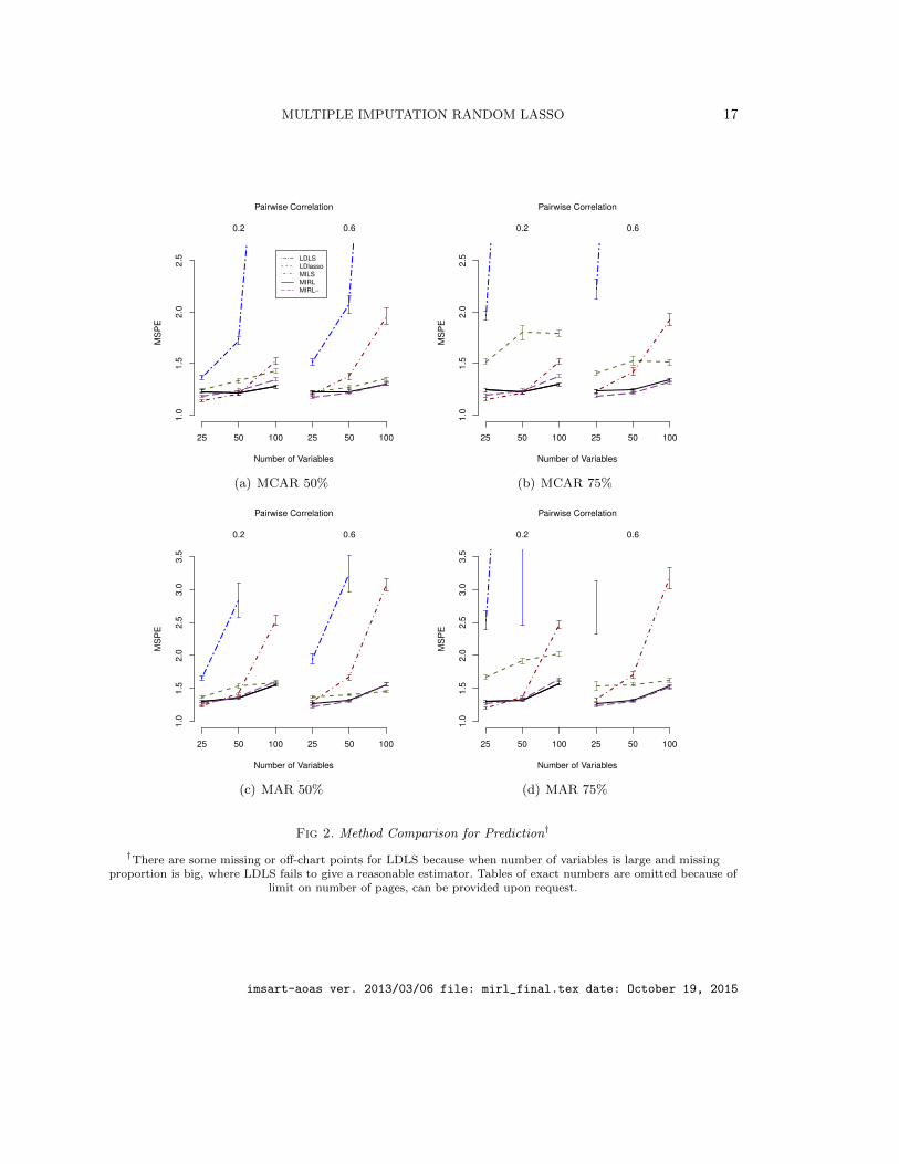
4.2. Simulation results. We present simulation results in Figures 2 and 3. Firstly, thesimulations demonstrate that stability selection enhances MIRL’s ability in variable selec-tion. MIRL− selects many noise variables, which may decrease the prediction accuracy.The MCC of MIRL− is much smaller than that of MIRL in almost all scenarios, whichshows that the stability selection step substantially improves the variable selection abilityof MIRL compared to the hard threshold used in the random lasso. As for the predictionperformance, MIRL has slightly larger MSPE than MIRL− for some scenarios with p = 25,although these differences are within the one standard error band. As the number of noisevariable increases, MIRL shows more significant advantages. For MCAR 50% and 75% withpairwise correlation 0.2 and p = 100 scenario, MIRL has significantly smaller MSPE thanMIRL− as presented in Figure 2 (a) and (b).

Secondly, the simulations show that the multiple imputation step makes better use of theavailable information than listwise deletion. MILS and MIRL are much better than LDLSin both MSPE and MCC in all scenarios. LDLS is not feasible when p is large and missingproportion is large because the sample size after listwise deletion is less than the numberof variables. LDlasso outperforms MIRL in the MAR scenario when p = 100, pairwisecorrelation 0.6 and missing proportion 50%. In this scenario, there is high correlationbetween all the informative variables and noise variables. MIRL selects more noise variablesthan LDlasso due to their correlation with important variables. When none or not all of thenoise variables are highly correlated with influential variables, MIRL is expected to showclear advantage. To demonstrate this, we run additional simulation and present results inFigure 4. The three scenarios are all MAR and the common missing proportion is 50%,the common pairwise correlation is 0.6. The number of variables is fixed to be 100 withdifferent numbers of noise variables correlated with informative ones, 0, 40, 90, respectively.We observe that when decreasing the number of noise variables correlated with informativeones, MCC increases for MIRL and decreases for LDlasso. For example, when there is nonoise variable correlated with informative variables, the MCC of LDlasso is 0.126, which is34.1% for MIRL. In the new scenarios, the MSPE of the two methods are not significantlydifferent.

Thirdly, MILS is MIRL’s closest competitor, and MIRL has comparative advantage overMILS when the number of variables is large and the correlation between variables arelarge. MIRL is significantly better than MILS in both MSPE and MCC when p = 100. Forsmaller number of variables, i.e. p = 50, MSPE of MIRL and MILS are not significantlydifferent when pairwise correlation is 0.2, but MIRL has significantly smaller MSPE than



MILS when the pairwise correlation is 0.6. Moreover, the increase of pairwise correlationdoes not affect the predictive ability of MIRL much, but it increases MSPE for MILS. Forexample, in Figure 2 (a), for MCAR 50% scenario with p = 50 and pairwise correlation 0.2,MSPE is 1.208 for MIRL and 1.205 for MILS; when pairwise correlation is 0.6, MSPE is1.226 for MIRL and 1.372 for MILS. In addition, for multiple imputation based methods,MSPE and MCC are not significantly different between two missing proportions 50% and75% with the other parameters fixed. Changing the missing data scheme from MCAR toMAR increases MSPE and decreases MCC; but this does not affect the ranking of methods.

4.3. Simulation summary. Compared with other existing methods, MIRL shows ad-vantages when the data have high proportion of missing and highly correlated influentialvariables. In addition, in contrast to alternative choices, MIRL has the advantage in scal-ing up to high-dimensional data with large n and p: MIRL uses a parallel algorithm suchthat it can be easily distributed in parallel to multiple computing cores and the results aresummarized in the end. Additional simulation results of comparisons with other existingmethods are provided in Appendix A.

5. Data Analyses of Project EAT.

5.1. Main analyses. Here we present analyses of the proposed MIRL and other methodsidentifying risk and protective factors for adolescent obesity in Project Eat. Because ofthe non-monotone and complicated missing structure, large number of missing variables,diverse types of variables, the application of Johnson et al. (2008) and Garcia et al. (2011)is difficult. Hence, we compared MIRL with LDLS, MILS and CW. The analysis of ProjectEAT data were stratified by gender for comparability with prior work (Larson et al., 2013).Our proposed method and competitors were applied to select the most important of the 62multi-contextual environmental predictors of BMI z-score among 1307 teenage boys and1486 teenage girls separately. The estimated coefficient are provided in Table 2 for boysand Table 3 for girls.

The MSPE are based on 500 replications with training and testing sets of equal sizes.The MSPEs of LDLS, MILS, CW, and MIRL are 1.2762(se = 0.0015), 1.2274(se =0.0021), 1.2291(se = 0.0022), and 1.2248(se = 0.0021) for boys; and 0.8447(se = 0.0015),0.8422(se = 0.0015), 0.8354(se = 0.0015), and 0.8393(se = 0.0015) for girls. LDLS yieldsthe largest MSPE, MILS is the second largest for both gender. MIRL has smaller MSPEthan CW for boys and slightly larger for girls. The empirical selection probability of MIRLnaturally provides a ranking of the variable importance as shown in Table 2. The rank-ing does not rely on a single tuning parameter from one model fit and thus it reducessensitivity of the model selection to the tuning parameter. The chosen variable set is there-fore more stable than those selected based on a single model. Cross validation with theone-standard-error rule chose selection probability threshold as 0.9 for both genders.

MIRL selected 9 variables for boys. In addition to Hispanic, Native American, and Asianboys having significantly higher BMI z-score, it showed that high social economic status is


10

a protective factor, higher parental weight status and weight of same gender friends wererisk factors. As shown in the original Project EAT investigation (Neumark-Sztainer et al.,2012; Larson et al., 2013), we found some reactive factors, such as more unhealthy food athome and higher parental pressure to eat are associated with lower BMI z-score and higherparental restriction of high-calorie food is associated with higher BMI z-score.

MIRL also picked 9 variables for girls. It picked 3 new variables compared with boys,which are family meal frequency, safety during the night and day as well as parental rolemodeling of food choices. Fewer family meal frequency , lack of safety for day and night,and poorer parental role modeling for food choice are selected as risk factors for higherBMI. The common influential risk factors chosen by MIRL for both genders include socialeconomic class, parental weight status, parental pressure to eat, parental restriction of high-calorie food, home unhealthy food availability, and weight status of same gender friend.The estimated effect direction and magnitude are close to boys’ estimates.

Consistent with the previous simulation results, MILS performed similarly with MIRL,since p = 62 is only a small fraction of n = 1307. For boys, in addition to the 9 variablespicked by MIRL, MILS also identified age and family meal frequency to be significantlyassociated with lower BMI z-score at level 0.05. The two additional variables chosen byMILS have > 80% selection probability estimated by MIRL. For girls, MILS also selected9 variables very close to MIRL selected, except it selected the variable encouragement toeat healthy foods (selection probability 89.6% by MIRL) , and missed the variable weightstatus same gender friends. MIRL was able to identify weight status same gender friendsfor both boys and girls while MILS would have missed that for girls. MILS also selected fewvariables with large selection probabilities from MIRL but not above the threshold 90%.

For both genders, CW selected all variables chosen by MIRL, as well as 10 additionalvariables for each gender. The variables it chose for girls were the top 19 ranked by MIRLwith the lowest selection probability 79.6%. For boys, the chosen set consists of top 14variables ranked by MIRL, as well as a few variables with lower selection probabilities,such as household food insecurity (55%) and black ethnicity group (53.7%).

LDLS identified 3 common variables for both genders, including parental pressure toeat, parental weight status and weight status of same sex friends which are also selectedby MIRL. It missed the other variables chosen by MIRL, MILS and CW, and selectedparental role modeling of food choices for boys, which is not picked by any other methodand with low selection probability from MIRL (31.1%). LDLS chose parental restriction ofhigh-calorie food for girls which is a common risk factor picked by other methods. Theseanalyses suggested that loss of information due to listwise deletion reduces the power toidentify some potentially important variables.

The magnitudes of the coefficients obtained directly from MIRL, MILS and CW canbe different for some variables. One reason is that MIRL’s coefficients are averaged acrossbootstrapped samples including zero for the variables either not sampled in step 3 orshrunk to 0 when applying lasso regression. Thus although we expect these coefficients tobe consistent asymptotically, for finite sample, the shrinkage effect for the magnitude of



covariates might be evident. The same phenomenon was observed for random lasso (Wanget al., 2011). One way to mitigate the difference is to refit the model using the selectedvariables as suggested in CW. We present the refitted coefficients in Table 2 and 3 forMIRL, MILS and LDLS, where we can see that the coefficients for the chosen variableshave the same signs, and MIRL and MILS results are close since they chose similar sets ofvariables. LDLS chose less number of variables. The difference of the magnitudes for therefitted variables are due to collinearity of covariates.

5.2. Subgroup analyses. Next, we compare the methods in a targeted subsample pre-viously identified as at high risk of being overweight (Larson et al., 2013). One strengthof Project EAT is its ethnically diverse sample including: 19% non-Hispanic White, 29%Black, 17% Hispanic, 20% Asian, 4% Native Americans, and 11% Mixed/Other as well asa large proportion of low-income adolescents. Hence, in addition to identifying risk andprotective factors for the whole population, it is feasible to identify risk factors among spe-cific at-risk ethnic population so that interventions can be targeted. Asian teenage boys inMinneapolis/St. Paul were found to have the largest secular increases in overweight statusgoing from 30% overweight in 1999 to 50% in 2010 (Neumark-Sztainer et al., 2012). Thusit is of interest to consider specifically risk and protective factors within the sub-sample ofn = 99 low social economic status (SES) Asian boys.

There were only 20 subjects with complete data which is less than the number of pre-dictors. We excluded SES, ethnicity indicators and 6 variables, which are degenerated inthis analysis. We compared MIRL, MILS, and CW where only MIRL identified an im-portant predictor. For MIRL, cross validation chose 90% as the threshold, and parentalweight status was identified with selection probability 91.2%. All other variables have se-lection probability lower than 80%. Parental weight status is a strong predictor from abehavioral genetics perspective (Kral and Faith, 2009) and it is also picked in the largersample analysis by all available methods. For MILS, the p-value of parental weight statusis 0.5188. Table B1 in the appendix presents coefficients from MIRL and MILS for the top10 variables with highest ranking in MIRL. The analysis for this subgroup demonstratesMIRL’s advantages when the variable number p is relatively large compared to the samplesize n: MIRL detected some influential variables while MILS and CW detected none. Theseresults are consistent with our simulation results where MIRL shows greater comparativeadvantages over MILS and other methods in the cases with larger p and smaller n.

6. Conclusion and Discussion. Here we propose a procedure to address missingdata issue in variable selection for high-dimensional data through multiple imputation.When the number of variables with missing is large, alternative methods to adjust formissingness (e.g., likelihood-based methods through EM algorithm or inverse probabil-ity weighting) become difficult or infeasible. Our simulation results show that for low-dimensional case (e.g., p = 25, n = 200), the least squares regression for multiply imputeddata (MILS) can outperform more sophisticated lasso-based variable selection methods.


12

However, when the dimension increases, the advantage of lasso-based methods can be sub-stantial. Regarding the influence of missing, the efficiency loss in terms of MSPE for acomplete data analysis is considerable even when missing proportion is moderate (e.g.,50% complete data left after listwise deletion).

MIRL is especially suitable for cases where the informative variables are likely to becorrelated and it performs adequately when the noise variables are correlated with theinformative ones. In this case, the bootstrap samples and random draw of variables ac-cording to the importance measure enable variables highly correlated with the outcome tohave high selection probability and other noise variables to have low selection probabilitydespite their correlation with the informative ones. Another advantage of MIRL lies in itsflexibility in dealing with many missing data structures and variable selection techniques.In the imputation step, other imputation approaches such as MCMC can replace MICE. Inthe second step where penalized regression for each bootstrap sample is performed, othermethods such as regression with SCAD penalty (Fan and Li, 2001) and elastic net penalty(Zou and Hastie, 2005) can be used instead of lasso. In addition, although we focus onMIRL using linear model for continuous outcomes, it can be easily extended to generalizedlinear models for categorical outcomes, Cox regression model for censored outcomes andmixed effects models for longitudinal outcomes.

One extension of MIRL is to consider mixed effects models to allow random effects (e.g.,class-specific random effects in Project EAT). Groll and Tutz (2014) proposed variableselection method to introduce L1 penalty in mixed effects model. A possible solution is toconduct variable selection with random effects for each bootstrapped samples of imputeddata, and combine coefficients from imputed data sets by taking the average. Furtherinvestigations are needed to draw inference for combining the multiply imputed correlateddata or bootstrapped sample.

Lastly, since MIRL combines random lasso (Wang et al., 2011) and stability selection(Meinshausen and Buhlmann, 2010) to analyze multiply imputed data, it is of interestto consider whether theorems developed for stability selection can be applied. Since theimputation is performed for the covariates in the deign matrix, the random errors are inde-pendent when treating design matrix X as fixed in a regression problem. It is conjecturedthat an adapted version of Theorem 2 in Meinshausen and Buhlmann (2010) can be used toprovide some insights for variable selection consistency of MIRL when the imputed designmatrices satisfy sparse eigenvalue Assumption 1 in Meinshausen and Buhlmann (2010).However, rigorous theoretical investigation of MIRL is beyond the scope of this work.

Acknowledgements. We would like to thank Dianne Neumark-Sztainer for providingthe motivating Project EAT dataset and useful feedback. The Project EAT was supportedby grant number R01HL084064 (D. Neumark-Sztainer, principal investigator) from theNational Heart, Lung, and Blood Institute. This work is supported in part by NIH grantsNS073671, NS082062 and NSF grant DMS-1308566. The authors would like to thank theeditor, the associate editor and the reviewers for their constructive comments which have



helped to improve the quality of this work.


14

Fig 1. Flowchart of the MIRL Algorithm

Input: A sample of n observations with p predictor variables with possiblemissing

Step 1. Impute the sample m times and standardize all variables

Step 2. For each imputed data set, generate B bootstrap samplesa) Compute lasso-OLS coefficients for each bootstrapped sampleb) Compute the importance measure for each of the p variables as the ab-solute value of the simple average of the m×B coefficients

Step 3.a) For each m × B dataset, randomly select p/2 variables with probabilityproportional to importance measures; compute lasso-OLS coefficients forp/2 variables and set the rest to be 0b) Average m×B coefficients to get initial MIRL estimates

Step 4.Compute empirical selection probabilities and chose probability thresholdby cross-validation, under which the MIRL estimates are set to be zero



Table 1Most Frequent (>=1%) Missing Patterns of Some Important Variables in Project EAT data (“X”

indicates non-missing and “.” indicates missing)

Variables % Missing Missing Patterns

Parental pressure to eat 18 X X . . X X X X XParental restriction of high-calorie food 18 X X . . X X X X .

Asian 0 X X X X X X X X XParental weight status 21 X X . . . . X X X

Home unhealthy food availability 0 X X X X X X X X XHispanic 0 X X X X X X X X X

Social economical status 5 X X X X X X . . XWeight status male friends 36 X . X . X . X . X

Native american 0 X X X X X X X X XMissing Pattern Percentage (%) 48 26 9 5 2 2 1 1 1

∗: Marginal missing proportion for each variable.


16

Table 2Comparison of MIRL with MILS, LDLS and CW for Project EAT data (Boys)

Variables MIRL MILS LDLS CWrefit raw est. Prob refit raw est. p-value refit raw est. p-value

Parental pressure to eat -0.2664 -0.1779 1.0000 -0.2604 -0.2676 < 0.0001 -0.1830 -0.1108 < 0.0001 -0.2633Parental restriction of high-calorie food 0.2166 0.2301 0.9980 0.2044 0.2001 < 0.0001 0 0.0303 0.0613 0.1804

Asian 0.1765 0.0843 0.9970 0.1727 0.1903 0.0001 0 0.2753 0.3189 0.1713Parental weight status 0.2117 0.1662 0.9960 0.2044 0.1925 < 0.0001 0.2175 0.0269 0.0341 0.1922

Home unhealthy food availability -0.1058 -0.1313 0.9610 -0.1017 -0.0875 0.0115 0 -0.0229 0.4993 -0.0981Hispanic 0.1361 0.0118 0.9595 0.1408 0.1312 0.0033 0 -0.1621 0.5623 0.1225

Social economical status -0.1090 -0.0787 0.9580 -0.1032 -0.0928 0.0187 0 -0.0200 0.7636 -0.0784Weight status male friends 0.0861 0.0985 0.9470 0.0861 0.0844 0.0258 0.1116 0.5116 0.0106 0.0862

Native american 0.0911 0.0383 0.9180 0.0825 0.1021 0.0092 0 0.5176 0.2762 0.0813

During the night and day 0 0.0567 0.8605 0 0.0559 0.0968 0 -0.0211 0.9227 0.0690Age 0 -0.0773 0.8230 -0.0774 -0.1281 0.0147 0 -0.0448 0.5384 -0.0753

Presence of convenience store in 800 m 0 -0.0539 0.8080 0 -0.1668 0.0503 0 -0.6854 0.1605 -0.0769Family meal frequency 0 -0.0143 0.8065 -0.0589 -0.0701 0.0411 0 0.0117 0.7446 -0.0559

Park/recreation space (% of area) 0 -0.0373 0.7925 0 -0.0518 0.1471 0 -0.3328 0.0523 -0.0458Encouragement to eat healthy foods 0 0.0144 0.7715 0 0.0721 0.0583 0 0.1106 0.2884 0

Presence of convenience store in 1200 m 0 0.0116 0.7640 0 0.0578 0.1062 0 -0.1481 0.6209 0.0563Number of male friends in sample 0 0.0161 0.7310 0 0.0497 0.2322 0 0.1559 0.1703 0.0407Sedentary behavior female friends 0 0.0043 0.6460 0 -0.0337 0.3895 0 0.0025 0.5103 0

During the night 0 -0.0167 0.6430 0 -0.0459 0.1724 0 -0.2547 0.1777 0Moderate-to-vigorous PA female friends 0 -0.0087 0.6360 0 -0.0196 0.6340 0 -0.0133 0.4987 -0.0459Parental time spent watching TV with 0 0.0305 0.6315 0 0.0352 0.3346 0 -0.0121 0.7611 0

Healthy food served at family meals 0 -0.0013 0.6045 0 -0.0447 0.2206 0 -0.0141 0.6569 0Fast-food frequency male friends 0 0.0101 0.5815 0 0.0696 0.1346 0 0.0447 0.1848 0

Household food insecurity 0 0.0405 0.5500 0 0.0207 0.5901 0 0.2160 0.2115 0.0349Limited variety of fruits and veges 0 -0.0425 0.5435 0 -0.0598 0.1744 0 -0.1286 0.3444 0

Black 0 -0.0210 0.5370 0 -0.0069 0.8864 0 -0.1754 0.5081 -0.0071Weight status female friends 0 0.0167 0.5200 0 0.0309 0.4901 0 0.1742 0.3890 0

Friends’ support for PA 0 -0.0069 0.5095 0 -0.0265 0.4385 0 -0.0050 0.9018 0Friends’ attitudes of eating healthy foods 0 0.0191 0.5080 0 0.0461 0.1860 0 0.0119 0.8967 0

. . .Parental role modeling of food choices 0 0.0015 0.3110 0 -0.0225 0.5766 -0.0392 -0.0542 0.0487 0

. . .

Table 3Comparison of MIRL with MILS, LDLS and CW for Project EAT data (girls)

Variables MIRL MILS LDLS CWrefit raw est. Prob refit raw est. p-value refit raw est. p-value

Social Economic Status -0.1037 -0.1206 1.0000 -0.1147 -0.0900 0.0022 0 -0.0700 0.1790 -0.0889Parental pressure to eat -0.2079 -0.2528 1.0000 -0.2068 -0.2150 <0.0001 -0.1830 -0.1023 < 0.0001 -0.2065

Parental restriction of high-calorie food 0.2191 0.2679 1.0000 0.2165 0.2317 <0.0001 0.2313 0.0443 0.0004 0.2160Parental weight status 0.1855 0.1646 1.0000 0.1987 0.1714 <0.0001 0.1994 0.0296 0.0065 0.1811

Home unhealthy food availability -0.1005 -0.1001 0.9960 -0.0888 -0.1060 0.0001 0 -0.0071 0.7479 -0.1007Family meal frequency -0.0776 -0.0814 0.9880 -0.0882 -0.0843 0.0011 0 -0.0364 0.1480 -0.0802

Weight status female friends 0.0735 0.0183 0.9360 0 0.0534 0.1434 0.0799 0.3500 0.0282 0.0540Safety during the night and day 0.0557 0.0470 0.9240 0.0518 0.0642 0.0161 0 0.2550 0.0922 0.0553

Parental role modeling of food choices -0.0410 -0.0211 0.9200 -0.0742 -0.0659 0.0311 0 -0.0105 0.6068 -0.0720

Hispanic 0 0.0338 0.8960 0 0.0478 0.1748 0 0.2774 0.2258 0.0497Encouragement to eat healthy foods 0 0.0043 0.8960 0.0787 0.0822 0.0066 0 0.0964 0.2165 0.0818

Schools commitment to promoting PA 0 -0.0243 0.8960 0 -0.0299 0.7120 0 -0.1069 0.6960 -0.0605Asian 0 -0.0458 0.8680 0 -0.0482 0.2300 0 0.1633 0.4959 -0.0507

Parental fast food intake 0 0.0280 0.8560 0 0.0414 0.1976 0 0.0242 0.6410 0.0372Presence of convenience store in 1200 m 0 0.0306 0.8560 0 0.0520 0.0592 0 0.2049 0.3285 0.0314Moderate-to-vigorous PA female friends 0 -0.0327 0.8440 0 -0.0522 0.0683 0 -0.0236 0.1632 -0.0383

Parental time spent supporting PA 0 0.0195 0.8080 0 0.0599 0.1410 0 0.0130 0.6853 0.0525Weight status male friends 0 0.0276 0.8080 0 0.0368 0.2137 0 0.1555 0.3021 0.0447

Park/recreation space (% of area) 0 -0.0516 0.7960 0 -0.0360 0.1927 0 -0.0467 0.7186 -0.0356Schools commitment to promoting healthy eating 0 -0.0143 0.7480 0 -0.1173 0.1330 0 0.0784 0.7962 0

TV during dinner 0 -0.0015 0.6760 0 0.0224 0.3769 0 0.0005 0.9931 0Limited variety of available fruits and vegetables 0 -0.0129 0.6480 0 -0.0375 0.2462 0 0.0589 0.5608 0

Students allowed to drink during class 0 0.0182 0.6440 0 0.0244 0.7891 0 -0.1200 0.8501 0Indoor campus PA facilities 0 -0.0042 0.6240 0 -0.0434 0.4623 0 -0.0819 0.4320 0

Home healthy food availability 0 -0.0141 0.6000 0 -0.0137 0.6533 0 -0.0299 0.2173 0Distance to nearest gym/fitness center (m) 0 -0.0055 0.5880 0 0.0288 0.2899 0 0.0870 0.4931 0

Poor quality of fruits or vegetables 0 -0.0205 0.5520 0 -0.0237 0.4762 0 -0.0704 0.5297 0Age 0 -0.0009 0.4520 0 -0.0516 0.2040 0 -0.0112 0.8407 0

Density of total crime incidents 0 0.0107 0.4440 0 0.0083 0.7629 0 0.0634 0.6367 0Native American 0 0.0068 0.4240 0 0.0207 0.4669 0 -0.0210 0.9548 0

. . .



Number of Variables

MS

PE

25 50 100 25 50 100

1.0

1.5

2.0

2.5

0.2 0.6

Pairwise Correlation

LDLS

LDlasso

MILS

MIRL

MIRL−

(a) MCAR 50%

Number of Variables

MS

PE

25 50 100 25 50 100

1.0

1.5

2.0

2.5

0.2 0.6


(b) MCAR 75%

Number of Variables

MS

PE

25 50 100 25 50 100

1.0

1.5

2.0

2.5

3.0

3.5

0.2 0.6


(c) MAR 50%

Number of Variables

MS

PE

25 50 100 25 50 100

1.0

1.5

2.0

2.5

3.0

3.5

0.2 0.6


(d) MAR 75%

Fig 2. Method Comparison for Prediction†

†There are some missing or off-chart points for LDLS because when number of variables is large and missingproportion is big, where LDLS fails to give a reasonable estimator. Tables of exact numbers are omitted because of

limit on number of pages, can be provided upon request.


18

Number of Variables

MC

C

25 50 100 25 50 100

0.0

0.2

0.4

0.6

0.8

1.0

0.2 0.6


LDLS

LDlasso

MILS

MIRL

MIRL−

(a) MCAR 50%

Number of Variables

MC

C

25 50 100 25 50 100

0.0

0.2

0.4

0.6

0.8

1.0

0.2 0.6


(b) MCAR 75%

Number of Variables

MC

C

25 50 100 25 50 100

0.0

0.2

0.4

0.6

0.8

1.0

0.2 0.6


(c) MAR 50%

Number of Variables

MC

C

25 50 100 25 50 100

0.0

0.2

0.4

0.6

0.8

1.0

0.2 0.6


(d) MAR 75%

Fig 3. Method Comparison for Variable Selection†

†Tables of exact numbers are omitted because of limit on number of pages, can be provided upon request.



(a) MSPE

(b) MCC

Fig 4. MAR scenario with p = 100, pairwise correlation 0.6 and missing proportion 50%imsart-aoas ver. 2013/03/06 file: mirl_final.tex date: October 19, 2015

20

APPENDIX A: FURTHER COMPARISONS WITH EXISTING LITERATURE

We compare MIRL with methods in Johnson et al. (2008), Garcia, Ibrahim and Zhu(2010a), Chen and Wang (2013) (CW), and RRstep under Rubin’s rule (e.g., stepwiseregression with p-value computed based on Rubin’s rule standard error). We follow thesame simulation settings reported in Johnson et al. (2008) and Garcia et al. (2010a). Theresults for the scenario in section 5.2 of Johnson et al. (2008) are presented in Table B7.We can see that MIRL, RRstep and MILS show good performance in variable selection andprediction in all four cases, and they outperform Johnson et al. (2008). MILS and RRstepperform similarly in this scenario and using stepwise selection does not lead to betterresults than one-step backward selection (MILS). The simulation results from section 4.1in Garcia et al. (2008) are shown in Table B8. MIRL outperforms all its competitors interms of variable selection. RRstep and MILS also have high MCC for scenario 1 and 3. CWgives good MSPE for scenario 2 but the MCC is small. In these simulation settings, CWtends to select more variables, where gains a larger true positives at the cost of selectingmore noise variables.

Table B9 presents simulation results comparing MIRL with RRstep and CW for p > ncases. The simulation settings contain two pairs of n and p: n = 50, p = 100 and n =100, p = 200. The coefficients for x1, x2, . . . xp are β = (3, 1.5, 0, 0, 2, 0, . . . , 0), σ = 3, X1

and X2 missing at random depending on X3 to X8 and outcome, and about 30% of subjectsremain after listwise deletion. In this case, MIRL outperforms the other two methods interms of smaller prediction error, and has similar performance in terms of MCC.



APPENDIX B: SIMULATION RESULTS

Table B1Results for p = 25 with pairwise correlation 0.2

Approx.% leftafter listwisedeletion

L1 L2 MSPE TP TN MCC

LDLS 1.705(0.044) 0.371(0.016) 1.363(0.021) 5.97(0.119) 14.16(0.097) 0.603(0.012)MILS 1.069(0.031) 0.154(0.008) 1.138(0.013) 7.38(0.095) 14.25(0.098) 0.725(0.012)

50% LD lasso cv 1.75(0.041) 0.289(0.014) 1.242(0.015) 8.4(0.147) 8.69(0.292) 0.437(0.017)MIRLnoSS 1.489(0.03) 0.21(0.009) 1.18(0.014) 9.51(0.063) 4.37(0.157) 0.301(0.013)

MIRL 1.407(0.03) 0.262(0.011) 1.227(0.016) 6.02(0.122) 14.82(0.061) 0.673(0.01)MCAR LDLS 3.086(0.073) 1.105(0.049) 1.969(0.044) 3.14(0.186) 14.3(0.104) 0.381(0.018)

MILS 1.119(0.032) 0.169(0.008) 1.153(0.012) 7.13(0.105) 14.32(0.091) 0.711(0.012)25% LD lasso cv 2.576(0.067) 0.64(0.027) 1.518(0.026) 6.35(0.263) 9.76(0.367) 0.324(0.019)

MIRLnoSS 1.541(0.032) 0.223(0.009) 1.188(0.014) 9.45(0.067) 4.33(0.171) 0.288(0.014)MIRL 1.473(0.035) 0.288(0.012) 1.243(0.015) 5.83(0.134) 14.82(0.052) 0.658(0.01)

LDLS 2.376(0.064) 0.701(0.032) 1.651(0.036) 4.4(0.16) 14.21(0.105) 0.474(0.016)MILS 1.431(0.035) 0.241(0.01) 1.229(0.015) 7.39(0.121) 13.54(0.115) 0.663(0.015)

50% LD lasso cv 2.192(0.052) 0.434(0.019) 1.373(0.02) 7.63(0.171) 8.92(0.352) 0.372(0.021)MAR MIRLnoSS 1.784(0.033) 0.302(0.011) 1.266(0.015) 9.41(0.065) 4.28(0.168) 0.283(0.014)

MIRL 1.654(0.036) 0.35(0.014) 1.31(0.016) 6.06(0.147) 14.62(0.09) 0.658(0.011)LDLS 3.747(0.151) 1.716(0.168) 2.53(0.143) 2.37(0.166) 14.1(0.138) 0.294(0.021)MILS 1.385(0.034) 0.234(0.01) 1.207(0.016) 7.33(0.129) 13.82(0.098) 0.681(0.015)


MIRL 1.67(0.034) 0.358(0.013) 1.304(0.017) 5.84(0.143) 14.73(0.066) 0.65(0.01)


22




LDLS 2.418(0.06) 0.724(0.03) 1.514(0.037) 4.28(0.156) 14.31(0.088) 0.475(0.016)MILS 1.536(0.037) 0.307(0.013) 1.203(0.017) 6.05(0.123) 14.38(0.089) 0.631(0.011)


MIRL 1.912(0.04) 0.46(0.018) 1.219(0.014) 5.21(0.171) 14.46(0.123) 0.576(0.013)MCAR LDLS 3.79(0.097) 1.694(0.09) 2.224(0.097) 1.87(0.147) 14.25(0.105) 0.248(0.017)

MILS 1.593(0.039) 0.337(0.014) 1.231(0.019) 5.8(0.123) 14.37(0.085) 0.609(0.012)25% LD lasso cv 3.02(0.071) 0.928(0.033) 1.407(0.019) 4.47(0.296) 11.4(0.326) 0.262(0.022)

MIRLnoSS 2.104(0.038) 0.414(0.015) 1.186(0.012) 9.27(0.074) 3.58(0.161) 0.212(0.016)MIRL 1.956(0.044) 0.483(0.02) 1.23(0.013) 4.97(0.181) 14.55(0.091) 0.569(0.014)

LDLS 3.207(0.065) 1.2(0.045) 1.942(0.076) 2.46(0.144) 14.32(0.089) 0.305(0.016)MILS 2.056(0.047) 0.487(0.018) 1.308(0.02) 6.07(0.128) 13.28(0.121) 0.528(0.014)


MIRL 2.073(0.039) 0.517(0.018) 1.264(0.015) 5.38(0.171) 13.97(0.118) 0.537(0.014)LDLS 4.125(0.176) 2.233(0.303) 2.735(0.402) 1.14(0.121) 14.23(0.114) 0.142(0.024)MILS 2.003(0.044) 0.476(0.017) 1.328(0.024) 5.96(0.133) 13.57(0.112) 0.545(0.013)


MIRL 2.06(0.04) 0.513(0.018) 1.272(0.016) 5.47(0.177) 14.02(0.114) 0.549(0.015)






LDLS 2.742(0.087) 0.796(0.036) 1.721(0.039) 4.87(0.166) 37.83(0.206) 0.512(0.016)MILS 1.403(0.036) 0.234(0.01) 1.205(0.015) 7.43(0.102) 38.22(0.135) 0.726(0.011)


MIRL 1.424(0.031) 0.253(0.01) 1.208(0.016) 6.83(0.105) 39.29(0.13) 0.75(0.01)MCAR LDLS 5.946(0.624) 6.475(1.443) 6.637(1.181) 0.875(0.215) 38.286(0.507) 0.175(0.042)

MILS 1.428(0.037) 0.245(0.011) 1.218(0.017) 7.16(0.104) 38.36(0.133) 0.714(0.011)25% LD lasso cv 3.539(0.186) 0.985(0.082) 1.799(0.066) 5.38(0.261) 30.56(0.845) 0.307(0.017)

MIRLnoSS 2.366(0.034) 0.299(0.009) 1.238(0.015) 9.59(0.057) 9.01(0.263) 0.188(0.008)MIRL 1.458(0.03) 0.266(0.01) 1.223(0.016) 6.59(0.114) 39.34(0.109) 0.734(0.01)

LDLS 4.179(0.238) 2.021(0.32) 2.837(0.258) 2.152(0.171) 38.152(0.239) 0.28(0.019)MILS 2.203(0.07) 0.446(0.019) 1.424(0.021) 7.14(0.119) 35.49(0.267) 0.581(0.015)


MIRL 1.891(0.043) 0.382(0.013) 1.35(0.017) 6.67(0.144) 37.24(0.351) 0.642(0.013)LDLS 5.303(1.752) 9.472(8.068) 10.149(7.689) 0(0) 40(0) NaN(NA)MILS 2.087(0.057) 0.428(0.017) 1.366(0.019) 6.89(0.117) 36.28(0.206) 0.591(0.013)


MIRL 1.893(0.041) 0.384(0.013) 1.321(0.016) 6.59(0.133) 37.28(0.344) 0.635(0.013)




LDLS 3.746(0.119) 1.44(0.067) 2.072(0.084) 3.39(0.16) 37.71(0.211) 0.365(0.019)MILS 2.043(0.055) 0.478(0.019) 1.372(0.031) 5.87(0.104) 37.99(0.162) 0.598(0.012)


MIRL 2.13(0.044) 0.472(0.016) 1.226(0.015) 6.07(0.146) 37.14(0.316) 0.588(0.011)MCAR LDLS 6.986(0.962) 9.495(2.528) 7.595(1.885) 0.607(0.178) 38.071(0.571) 0.059(0.035)

MILS 2.064(0.056) 0.496(0.02) 1.422(0.035) 5.62(0.099) 38.12(0.153) 0.586(0.011)25% LD lasso cv 3.782(0.183) 1.245(0.103) 1.521(0.044) 3.65(0.274) 32.97(0.742) 0.249(0.017)

MIRLnoSS 3.099(0.045) 0.517(0.015) 1.218(0.014) 9.54(0.063) 8.01(0.281) 0.163(0.009)MIRL 2.158(0.045) 0.48(0.015) 1.243(0.014) 6.09(0.141) 37.05(0.384) 0.592(0.013)

LDLS 5.375(0.316) 3.631(0.422) 3.238(0.278) 1.273(0.129) 38.071(0.277) 0.169(0.022)MILS 3.287(0.094) 0.921(0.035) 1.667(0.042) 5.53(0.142) 34.92(0.242) 0.425(0.016)


MIRL 2.778(0.067) 0.651(0.021) 1.324(0.016) 6.32(0.169) 33.3(0.564) 0.462(0.015)LDLS NaN(NA) NaN(NA) NaN(NA) NaN(NA) NaN(NA) NaN(NA)MILS 3.248(0.088) 0.914(0.034) 1.704(0.046) 5.36(0.138) 35.24(0.217) 0.421(0.015)


MIRL 2.757(0.064) 0.645(0.021) 1.326(0.016) 6.22(0.174) 33.36(0.564) 0.455(0.015)


24




LDLS 6.662(0.946) 5.162(1.031) 6.018(1.106) 0.739(0.212) 86.283(1.332) 0.104(0.033)MILS 2.466(0.078) 0.544(0.021) 1.526(0.029) 6.43(0.111) 85.39(0.307) 0.583(0.012)


MIRL 1.745(0.041) 0.311(0.011) 1.273(0.015) 7.1(0.095) 87(0.302) 0.689(0.009)MCAR LDLS NaN(NA) NaN(NA) NaN(NA) NaN(NA) NaN(NA) NaN(NA)

MILS 2.374(0.075) 0.533(0.021) 1.517(0.028) 6.18(0.111) 86.05(0.282) 0.586(0.012)25% LD lasso cv 3.551(0.105) 0.946(0.028) 1.794(0.032) 4.01(0.24) 79.11(1.04) 0.294(0.013)

MIRLnoSS 3.712(0.049) 0.429(0.012) 1.376(0.016) 9.49(0.064) 21.4(0.476) 0.136(0.005)MIRL 1.761(0.044) 0.325(0.012) 1.299(0.016) 6.92(0.099) 87.23(0.373) 0.688(0.009)

LDLS NaN(NA) NaN(NA) NaN(NA) NaN(NA) NaN(NA) NaN(NA)MILS 6.023(0.204) 1.737(0.072) 2.535(0.071) 5.87(0.134) 75.02(0.645) 0.326(0.014)




MIRL 3.015(0.082) 0.664(0.02) 1.579(0.023) 6.26(0.163) 80.18(0.848) 0.467(0.014)




LDLS 8.317(1.357) 8.944(1.951) 7.478(1.716) 0.63(0.187) 86.261(1.273) 0.079(0.032)MILS 3.576(0.11) 1.136(0.044) 1.959(0.077) 4.64(0.128) 85.5(0.292) 0.444(0.013)


MIRL 2.633(0.077) 0.571(0.019) 1.303(0.018) 6.02(0.146) 82.37(0.912) 0.506(0.013)MCAR LDLS NaN(NA) NaN(NA) NaN(NA) NaN(NA) NaN(NA) NaN(NA)

MILS 3.404(0.101) 1.095(0.043) 1.927(0.059) 4.34(0.124) 86.21(0.258) 0.444(0.013)25% LD lasso cv 3.829(0.148) 1.193(0.048) 1.509(0.025) 2.29(0.241) 82.56(1.03) 0.209(0.018)

MIRLnoSS 4.827(0.063) 0.715(0.02) 1.316(0.016) 9.31(0.072) 17.86(0.439) 0.099(0.007)MIRL 2.639(0.071) 0.587(0.02) 1.338(0.018) 5.97(0.138) 82.93(0.796) 0.505(0.013)

LDLS NaN(NA) NaN(NA) NaN(NA) NaN(NA) NaN(NA) NaN(NA)MILS 9.291(0.248) 3.574(0.122) 3.08(0.092) 4.4(0.162) 72.09(0.597) 0.18(0.013)




MIRL 4.957(0.137) 1.16(0.036) 1.531(0.025) 6.11(0.21) 64.59(1.637) 0.245(0.014)



Table B7Comparison for Johnson’s Scenario

L1 L2 MPSE TP TN MCC

MILS 0.52 0.07 1.07 5.65 3.81 0.90LDlasso 0.97 0.16 1.15 5.98 1.73 0.62

Setting 1 MIRL 0.65 0.11 1.09 5.30 3.84 0.85σ = 1 CW 0.59 0.07 1.06 5.99 2.75 0.75

RRstep 0.56 0.08 1.06 5.63 3.85 0.90JohnLas 5.91 2.42 0.67

JohnALas 5.77 3.55 0.86

MILS 1.08 0.30 1.25 4.92 3.81 0.76LDlasso 2.37 1.02 2.08 5.67 2.01 0.57

Setting 1 MIRL 1.28 0.40 1.31 4.75 3.87 0.76σ = 2 CW 1.10 0.23 1.17 5.70 2.89 0.71

RRstep 1.13 0.28 1.19 5.07 3.79 0.78JohnLas 4.88 3.70 0.72

JohnALas 5.60 2.54 0.61

MILS 0.29 0.04 1.03 3.00 6.67 0.94LDlasso 0.87 0.16 1.14 3.00 3.48 0.52

Setting 2 MIRL 0.27 0.03 1.02 3.00 6.60 0.95σ = 1 CW 0.48 0.06 1.04 3.00 4.95 0.66

RRstep 0.31 0.04 1.03 3.00 6.63 0.93JohnLas 3.00 4.11 0.55

JohnALas 3.00 6.25 0.85

MILS 0.56 0.15 1.15 3.00 6.64 0.93LDlasso 2.14 0.99 2.01 3.00 3.79 0.55

Setting 2 MIRL 0.50 0.10 1.12 3.00 6.69 0.95σ = 2 CW 0.85 0.19 1.18 3.00 5.02 0.67

RRstep 0.54 0.12 1.13 3.00 6.72 0.95JohnLas 2.98 4.56 0.59

JohnALas 2.98 6.08 0.81


26

Table B8Comparison for Garcia’s Scenario

L1 L2 MPSE TP TN MCC

MILS 1.04 0.58 1.67 2.98 4.87 0.97LDlasso 1.57 0.59 1.56 3.00 2.24 0.54

n = 40 MIRL 1.21 0.65 1.77 2.98 4.83 0.98σ = 1 CW 1.72 0.77 1.81 3.00 3.09 0.64

RRstep 1.31 0.72 1.75 2.96 4.80 0.95GarciaAlasso 3.00 4.64 0.91GarciaSCAD 3.00 4.64 0.91

MILS 3.75 6.26 6.67 2.07 4.76 0.73LDlasso 5.20 6.32 7.31 2.74 2.65 0.50

n = 40 MIRL 3.82 5.55 6.31 2.24 4.71 0.80σ = 3 CW 3.77 3.94 4.40 2.93 3.49 0.68


MILS 0.87 0.38 1.33 2.99 4.76 0.95LDlasso 1.30 0.39 1.34 3.00 2.48 0.62

n = 60 MIRL 0.86 0.31 1.29 2.99 4.98 0.99σ = 1 CW 1.31 0.45 1.40 3.00 3.24 0.65


Table B9p > n case for 100 replications

Settings L1 L2 MPSE TP TN MCC

n = 50 MIRL 9.55 16.51 19.50 1.12 92.93 0.27p = 100 RRstep 14.01 25.78 26.23 1.23 91.22 0.27

CW 35.94 42.04 42.15 2.65 43.32 0.13

n = 100 MIRL 10.03 13.59 15.67 1.74 187.48 0.31p = 200 RRstep 18.36 25.04 24.71 1.62 182.22 0.25

CW 24.96 28.15 27.95 2.26 153.72 0.35



APPENDIX C: SUBGROUP ANALYSIS

Table B1MIRL Selected Sequence of Important Variables Compared with MILS Selection for Boys

Variables MIRL MILSraw est. Prob raw est. p-value

Parental weight status 0.0689 0.9115 0.2347 0.5188

Distance to nearest recreation center(m) -0.1039 0.7950 -0.2779 0.3471Competitive food with policies -0.1286 0.7590 -0.3597 0.5438

Park/recreation space (% of area) -0.0035 0.7160 -0.0437 0.8842Poor quality of fruits/vegetables 0.0386 0.7060 0.0038 0.9904

Friends’ attitudes of eating healthy foods 0.0359 0.7030 0.4056 0.1383During the night -0.1511 0.6985 -0.2100 0.6564

TV during dinner -0.1696 0.6715 -0.4001 0.0751Fast-food frequency male friends -0.0719 0.6630 -0.3674 0.3973

Number of male friends in sample 0.0344 0.6255 -0.0505 0.8755Parental fast food intake 0.0382 0.5975 -0.0226 0.9333


28

REFERENCES

Azur, M. J., Stuart, E. A., Frangakis, C. and Leaf, P. J. (2011). Multiple Imputation by Chained Equations:What isit and how does it work? Int J Methods Psychiatr Res. 20 40-49.

Belloni, A. and Chernozhukov, V. (2013). Least squares after model selection in high-dimensional sparse modes.Bernoulli 19 521547.

Breiman, L. (2001). Random forests. Machine learning 45 5–32.Chen, Q. and Wang, S. (2013). Variable selection for multiply-imputed data with application to dioxin exposure study.

Statistics in medicine 32 3646-59.Claeskens, G. and Consentino, F. (2008). Variable Selection with Incomplete Covariate Data. Biometrics 64 1062-1069.Derksen, S. and Keselman, H. (1992). Backward, forward and stepwise automated subset selection algorithms: Frequency

of obtaining authentic and noise variables. British Journal of Mathematical and Statistical Psychology 45 265–282.Efron, B., Hastie, T., Johnstone, I. and Tibshirani, R. (2004). Least angle regression. The Annals of statistics 32

407–499.Fan, J. and Li, R. (2001). Variable Selection via Nonconcave Penalized Likelihood and its Oracle Properties. Journal of the

American Statistical Association 96 1348-1360.Frerichs, L., Perin, D. M. P. and Huang, T. T.-K. (2012). Current trends in childhood obesity research. Current

Nutrition Reports 1 228–238.Garcia, R. I., Ibrahim, J. G. and Zhu, H. (2010a). Variable Selection for Regression Models with Missing Data. Stat Sin.

20 149-165.Garcia, R. I., Ibrahim, J. G. and Zhu, H. (2010b). Variable selection in the cox regression model with covariates missing

at random. Biometrics 66 97-104.Glynn, R. J., Laird, N. M. and Rubin, D. B. (1993). Multiple imputation in mixture models for nonignorable nonresponse

with follow-ups. Journal of the American Statistical Association 88 984–993.Groll, A. and Tutz, G. (2014). Variable selection for generalized linear mixed models by l 1-penalized estimation. Statistics

and Computing 24 137–154.Hurvich, C. M. and Tsai, C. (1990). The impact of model selection on inference in linear regression. The American

Statistician 44 214–217.Ibrahim, J. G., Zhu, H., Garcia, R. I. and Guo, R. (2011). Fixed and Random Effects Selection in Mixed Effects Models.

Biometrics 67 495–503.Johnson, B. A., Lin, D. Y. and Zeng, D. (2008). Penalized Estimating Functions and Variable Selection in Semiparametric

Regression Models. Journal of the American Statistical Association 103 672-680.Kral, T. V. and Faith, M. S. (2009). Influences on child eating and weight development from a behavioral genetics

perspective. Journal of pediatric psychology 34 596–605.Laird, N. M. and Ware, J. H. (1982). Random-effects models for longitudinal data. Biometrics 963–974.Larson, N. I., Wall, M. M., Story, M. T. and Neumark-Sztainer, D. R. (2013). Home/family, peer, school, and

neighborhood correlates of obesity in adolescents. Obesity 21 1858-69.Matthews, B. W. (1975). Comparison of the predicted and observed secondary structure of T4 phage lysozyme. Biochimica

et Biophysica Acta (BBA) - Protein Structure 405 442 - 451.Meinshausen, N. and Buhlmann, P. (2010). Stability Selection. Journal of the Royal Statistical Society Series B 72

417-473.Neumark-Sztainer, D., Wall, M. M., Larson, N., Story, M., Fulkerson, J. A., Eisenberg, M. E. and Hannan, P. J.

(2012). Secular trends in weight status and weight-related attitudes and behaviors in adolescents from 1999 to 2010.Preventive medicine 54 77–81.

Rubin, D. B. (1987). Multiple Imputation for Nonresponse in Surveys. Wiley:New York.Shen, C. and Chen, Y. (2012). Model Selection for Generalized Estimating Equations Accommodating Dropout Missingness.

Biometrics 68 1046-54.Siddique, J. and Belin, T. R. (2008). Using an Approximate Bayesian Bootstrap to Multiply Impute Nonignorable Missing

Data. Computational Statistics & Data Analysis 53 405-415.Tibshirani, R. (1996). Regression Shrinkage and selection via the lasso. Journal of Royal Statistics Society Series B 58

267-288.Wang, S., Nan, B., Rosset, S. and Zhu, J. (2011). Random Lasso. Annals of Applied Statistics 5 468-485.Wood, A. M., White, I. R. and Royston, P. (2008). How should variable selection be performed with multiply imputed

data? Statist. Med. 27 3227-3246.Zou, H. and Hastie, T. (2005). Regularization and variable selection via the elastic net. Journal of the Royal Statistical

Society: Series B (Statistical Methodology) 67 301–320.



Ying LiuDepartment of BiostatisticsColumbia University722 West 168th StreetNew York, NY 10032E-mail: [email protected]

Yang FengDepartment of StatisticsColumbia University1255 Amsterdam Ave.10th Floor, MC 4690New York, NY 10027E-mail: [email protected]

Yuanjia WangDepartment of BiostatisticsColumbia University630 West 168th StreetNew York, NY 10032E-mail: [email protected]

Melanie M. WallDepartment of BiostatisticsColumbia University630 West 168th StreetNew York, NY 10032E-mail: [email protected]


VARIABLE SELECTION AND PREDICTION WITH INCOMPLETE …yl2802/mirl_final.pdf · VARIABLE SELECTION...

Documents

Transcript of VARIABLE SELECTION AND PREDICTION WITH INCOMPLETE …yl2802/mirl_final.pdf · VARIABLE SELECTION...