IZA DP No. 3697

Variable Search Intensity in an Economy withCoordination Unemployment

Leo Kaas

DI

SC

US

SI

ON

PA

PE

R S

ER

IE

S

Forschungsinstitutzur Zukunft der ArbeitInstitute for the Studyof Labor

September 2008

Variable Search Intensity in an

Economy with Coordination Unemployment

Leo Kaas University of Konstanz

and IZA

Discussion Paper No. 3697 September 2008

IZA

P.O. Box 7240 53072 Bonn

Germany

Phone: +49-228-3894-0 Fax: +49-228-3894-180

E-mail: iza@iza.org

Any opinions expressed here are those of the author(s) and not those of IZA. Research published in this series may include views on policy, but the institute itself takes no institutional policy positions. The Institute for the Study of Labor (IZA) in Bonn is a local and virtual international research center and a place of communication between science, politics and business. IZA is an independent nonprofit organization supported by Deutsche Post World Net. The center is associated with the University of Bonn and offers a stimulating research environment through its international network, workshops and conferences, data service, project support, research visits and doctoral program. IZA engages in (i) original and internationally competitive research in all fields of labor economics, (ii) development of policy concepts, and (iii) dissemination of research results and concepts to the interested public. IZA Discussion Papers often represent preliminary work and are circulated to encourage discussion. Citation of such a paper should account for its provisional character. A revised version may be available directly from the author.

IZA Discussion Paper No. 3697 September 2008

ABSTRACT

Variable Search Intensity in an Economy with Coordination Unemployment*

This paper analyzes an urn-ball matching model in which workers decide how intensively they sample job openings and apply at a stochastic number of suitable vacancies. Equilibrium is not constrained efficient; entry is excessive and search intensity can be too high or too low. Moreover, an inefficient discouraged-worker effect among homogenous workers emerges under adverse labor market conditions. Unlike existing coordination-friction economies with fixed search intensity, the model can account for the empirical relation between the job-finding rate and the vacancy-unemployment ratio, provided that search costs are small and that search intensity is sufficiently procyclical. JEL Classification: E24, J63, J64 Keywords: matching function, coordination frictions, unemployment Corresponding author: Leo Kaas Department of Economics University of Konstanz Box D145 78457 Konstanz Germany E-mail: Leo.Kaas@uni-konstanz.de

* I am grateful to Pieter Gautier and to audiences at the Penn S&M workshop, the NBER Summer Institute 2008, and at the Universities of Bonn and Vienna for their comments. Support by the German Research Foundation is gratefully acknowledged.

1 Introduction

Search and matching models are widely used to address various labor market phe-

nomena, such as unemployment, worker and job flows, and wage dispersion. A large

portion of the literature utilizes the idea of a reduced–form matching function which

maps the stocks of searching workers and firms into the flow of new matches. Despite

of its modeling advantages, this approach suffers from two limitations. One is its

inability to deal with heterogeneity convincingly. Of course, the foremost purpose of

the matching function is to abstract from any explicit source of frictions (including

heterogeneity) to describe the implications of costly trading in the labor market with

a minimum amount of complexity. Yet, many important issues (for example, the

pattern of skill premia) require an explicit analysis of how heterogeneity affects labor

market outcomes.1 The other limitation is that a reduced–form matching function

is, by construction, invariant to policy. Again a more explicit model of frictions

is needed to address how policy affects the matching relationship (see also Lagos

(2000) and Shimer (2007)).

There is a large literature on microeconomic foundations behind the aggregate

matching function; see section 3 of Petrongolo and Pissarides (2001) for a survey.

One such foundation rests on coordination frictions; early contributions are Butters

(1977), Hall (1977) and Montgomery (1991), more recent ones are Burdett, Shi, and

Wright (2001), Julien, Kennes and King (2000, 2006) and Albrecht, Gautier, and

Vroman (2006). The key idea is simple: since workers do not coordinate their ap-

plication decisions and firms do not coordinate their job–offer decisions, some firms

end up with no applications while others get many, and some workers obtain several

job offers while others have none. So at the end of every period, unfilled jobs and

unemployed workers coexist. These models give rise to aggregate matching functions

which typically have constant returns in economies with a large number of workers

and jobs.

Still there are a few open issues with coordination–friction models. One is that search

intensity is typically held constant. Although it is straightforward to include variable

1There is a number of papers utilizing reduced–form matching functions in models with het-

erogenous jobs or heterogenous skills (e.g. Acemoglu (2001) and Albrecht and Vroman (2002)).

But such models must rest on ad–hoc assumptions on how workers and jobs of different types are

matched.

1

search intensity in standard search models with exogenous matching functions (see

Chapter 5 of Pissarides (2000)), it is a less obvious matter in economies where

matching frictions result explicitly from coordination problems. Work by Albrecht,

Gautier, and Vroman (2006), Galenianos and Kircher (2008) and Kircher (2007)

identifies search intensity with the number of applications that a worker sends.

However, because of the discrete–choice nature of the worker’s decision problems,

equilibrium is difficult to characterize analytically. Also it is not obvious whether

the number of applications is the right measure for search intensity. Chance plays an

important role in the search for jobs; some workers who search hard may simply be

unlucky, find few suitable job openings and send few applications. Others who spend

less time on search, may notice a larger number of adequate job openings and send

more applications. A second open issue is quantitative: can coordination–friction

models match the empirical relation between the vacancy–unemployment ratio and

the job–finding rate? Recently, Mortensen (2007) and Shimer (2007) have analyzed

microfoundations of the matching function which are based on mismatch and which

generate a reasonable fit of the matching function and of the Beveridge curve. To

my knowledge, these quantitative features have not been explored for models with

coordination frictions thus far.2

This paper addresses these two issues. The first contribution is theoretical and is the

content of Section 2. I analyze an urn–ball matching model in which workers decide

about the rate at which they sample job openings (“search intensity”) and apply

at all suitable jobs they observe. For a given search intensity, the actual number

of suitable jobs (and so the number of applications) is stochastic. The expected

number of applications, however, increases proportionately with search intensity.

As applications are sent randomly, wages are determined by ex–post competition,

according to the same bidding game as in Julien, Kennes and King (2000, 2006) and

Albrecht, Gautier, and Vroman (2006). Workers with at least two offers receive the

competitive wage, those who have only one offer are paid the reservation wage. A key

advantage of my model is that search intensity is a continuous choice variable, which

makes the model tractable and allows for an explicit equilibrium characterization

using first–order conditions. When labor market conditions are good, there are many

job openings per worker and all workers search with the same intensity. With less

2Julien, Kennes, and King (2006) examine a coordination–friction model quantitatively, but

their focus is wage dispersion, and not the matching–function elasticity.

2

favorable conditions, however, there are fewer job openings and it may happen that

no symmetric equilibrium in pure search–intensity strategies exists. Instead, some

workers are active and search with a common positive intensity, while others remain

inactive and decide not to search at all. Thus, the model can describe endogenous

nonparticipation in an environment where all workers are equally productive and

have the same taste for leisure. When comparing these equilibrium outcomes to

the choice of a social planner, I obtain the following results: (i) nonparticipation is

never constrained efficient; (ii) entry is always excessive, for the same reason as in

Albrecht, Gautier, and Vroman (2006), and (iii) search intensity can be too high or

too low.

Section 3 contains the quantitative exploration of this model. In Section 3.1 I

show that existing coordination–friction models, with fixed search intensity and

with a reasonable choice of the period length, are unable to account for the empirical

elasticity of the matching function. Specifically, the job–finding rate responds too

little to variations in the vacancy–unemployment ratio. I then go on to examine

a dynamic version of my model in which the parameters of a reduced–form search

cost function are calibrated so as to match both the mean job–finding rate and its

elasticity with respect to the vacancy–unemployment ratio. I find that search costs

are quantitatively small (less than 1% of the utility flow of an unemployed worker)

but search intensity responds strongly and positively to productivity. Nonetheless,

variable search intensity amplifies the economy’s reaction to a productivity shock

only little.

2 The static model

2.1 The setup

Consider a one–period economy with a large number M of identical workers and

a large number of N of identical firms, each creating one vacancy. The number of

workers is fixed, but the number of firms is determined from a free–entry condition.

I consider the limit where both M and N tend to infinity and where q = M/N ,

the number of workers per job opening, is positive and finite. All agents are risk

neutral and aim to maximize their expected income net of search costs. At the end

of the period, unemployment income is zero and employed workers produce p units

3

of output (=job surplus). I consider the following sequence of events.

Stage I Firms enter at marginal cost c(1/q) where c is a weakly increasing function

of the number of active firms per worker.

Stage II Every worker decides search intensity λ at cost k(λ), where k is increasing

and convex in λ ≥ 0. If a worker searches with intensity λ, he observes a

suitable vacancy at any given firm with probability λ/N and applies there.

These stochastic events are independent across workers and firms.

Stage III Each firm makes a wage offer to at most one applicant, rejecting all

others.

Stage IV Workers credibly reveal to firms how many offers they have, and firms

can simultaneously revise their initial bids.

Stage V Workers decide what offer (if any) to accept.

I impose the usual anonymity restriction that every worker treats all (identical)

firms equally (at stage V) and that every firm treats all workers equally (at stage

III).

Two remarks are in order. First, the specification that marginal entry costs are

not constant is needed to limit entry in an equilibrium where some workers are

inactive. The assumption can be justified, for example, by non–labor inputs in fixed

supply (e.g. land) whose prices increase in the number of active firms. Second,

search intensity is a continuous variable which determines the likelihood λ/N that

a worker observes a suitable job opening at any firm. This likelihood is plausibly

proportional to 1/N : the worker samples a certain (random) segment of the labor

market whose size increases with search intensity λ. If the number of firms becomes

larger, the size of the sampled segment stays the same, but the probability that a

given firm belongs to this segment falls with factor 1/N .

In the large economy, the number of applications (per worker and per job) are

Poisson distributed. A worker with search intensity λ applies at exactly n firms

with probability(

Nn

)(

λN

)n(

N − λN

)N−n≈ 1

n!λne−λ .

4

Conversely, if all workers search with intensity λ, a firm receives applications from

exactly m workers with probability

(

Mm

)(

λN

)m(

N − λN

)M−m≈ 1

m! (λq)me−λq .

Thus the expected number of applications per worker is λ and the expected number

of applications per firm is λq.

The last three stages of this game have the following solution. Firms offer the

reservation wage at stage III, revising the offer at stage IV only if the worker reveals

another offer, in which case Bertrand competition drives wage offers to the marginal

product. At the last stage, anonymity implies that workers randomize between

equal offers. In this respect, my model resembles those of Julien, Kennes, and King

(2000) and Albrecht, Gautier, and Vroman (2006) where workers with only one offer

are paid the monopsony wage and workers with multiple offers receive marginal

product. The setting of Julien et al. is the limiting case of my model where k(.) = 0

and λ/N = 1, so that every worker applies at all jobs. In the model of Albrecht et

al. all workers send the same number of applications. Here, in contrast, the number

of applications is stochastic, reflecting the role of chance in the search process.

Workers do not decide at how many firms they apply, but rather how intensively

they sample job openings. The model of Albrecht et al. also has an (irrelevant)

wage posting stage prior to the application stage where firms commit to a lower

wage bound which coincides in equilibrium with the reservation wage. My model

has a different interpretation in that workers do not observe any job postings at

the outset. Only after sampling, they apply to all suitable vacancies at zero cost.

Therefore search in this model is random rather than directed.3

2.2 The matching function

Before solving the model, it is useful to consider the matching function of this model.

Suppose, for the time being, that all workers decide the same search intensity λ at

stage II. For any worker i the probability to get an offer from firm j, conditional on

3Nonetheless, in an extension of this model with heterogenous job types, workers might “direct

search” by deciding how intensively they sample jobs of different types.

5

i applying at j, is4

z ≡ 1 − e−λq

λq .(1)

Hence, for any worker the probability to receive at least one offer (and thus to find

a job) is

∑

n≥1

1n!λ

ne−λ[

1 − (1 − z)n]

= 1 − e−λz = 1 − e−1−e−λq

q ≡ m(q, λ) .(2)

The matching rate for workers is increasing and concave in the job–worker ratio

1/q (as usual), and it is strictly increasing in λ: the more applications workers

send on average, the more likely it is that every worker receives an offer. Such a

result is not obvious; in fact it does not hold in the model of Albrecht, Gautier,

and Vroman (2006) where the matching rate can be declining in the fixed (non–

stochastic) number of applications. The reason for their result is that there are two

coordination frictions with multiple applications. The first friction is based on lack

of coordination between workers: some firms receive no applications while others

receive multiple applications since workers do not coordinate at the application

stage. The second friction is due to a lack of coordination between firms at the

job offer stage: some workers do not receive any offer, others have multiple offers.

Raising the number of applications mitigates the first friction but aggravates the

second one: it becomes more likely that multiple firms contact the same worker. In

my model the first effect always dominates so that the number of matches is globally

increasing in the common search intensity.

When λ → ∞, workers apply at all firms at stage I and the matching function is

mJ(q) ≡ 1− e−1/q, the same as in the model of Julien, Kennes, and King (2000). In

this limit only the second coordination friction is at work. In the model of Albrecht

et al. (2006), the matching function is mA(q, a) ≡ 1− [1− (1− e−aq)/(aq)]a when all

workers send a applications; again the matching function of Julien et al. emerges as

the special case a → ∞. For finite a, it may be that mA(q, a) > mJ(q), so matching

is more efficient with fewer applications. In my model, in contrast, matching is

always more efficient the more applications are sent, i.e. m(q, λ) < mJ(q) holds for

finite λ. It can also be shown that m(q, λ) < mA(q, λ); matching is more efficient

4The derivation is standard: Prob(i gets offer from j | i applies at j)Prob(i applies at j)= z ·λ/N

is equal to Prob(j gets ≥ 1 appl.)Prob(i gets offer from j | j gets ≥ 1 appl.)= (1 − e−λq) · 1/M .

Solving yields z.

6

when all workers send the same number of applications a = λ than when they

randomize applications from a Poisson distribution with mean λ.

2.3 Equilibrium search intensity

Consider the search intensity decision of workers at stage II after firm entry, so the

worker–job ratio q is given. A worker obtains income p if he receives two or more

offers at stage III, but he ends up with zero income otherwise. The probability to

have two or more offers, conditional on n applications, is

1 − (1 − z)n − nz(1 − z)n−1 .

When the worker’s search intensity is λ, the probability to end up with at least two

offers is

∑

n≥2

1n!λ

ne−λ[

1 − (1 − z)n − nz(1 − z)n−1]

= 1 − e−λz(1 + λz) .

When an individual worker in a large market decides λ, he takes z (the probability

to get an offer, conditional on applying) as given. Hence every worker solves

maxλ≥0

Uz(λ) ≡[

1 − e−λz(1 + λz)]

p − k(λ) .

This objective function is typically not concave; for many cost functions it is convex

at low values of λ and concave at higher values. Moreover, λ = 0 is always a local

maximum when k′(0) > 0 holds. An interior (i.e. active search) local maximum

must satisfy the first–order condition U ′z(λ) = 0, which is

k′(λ) = λz2e−λzp .(3)

Whenever there exists a pure–strategy equilibrium where all workers choose the same

search intensity λ∗ > 0, it follows from (1) and (3) that λ∗ solves

k′(λ) =(1 − e−λq)2e−

1−e−λq

q

λq2 p .(4)

To obtain analytical results, consider the uniformly elastic search cost function

k(λ) = kλ1+a/(1 + a) with a ≥ 0 and k > 0. Provided that the elasticity is large

enough (i.e. the function is sufficiently convex), a unique pure strategy equilibrium

must exist.

7

Proposition 1: Let k(λ) = kλ1+a/(1 + a) with a > 1. Then, for any given q, there

exists a unique equilibrium of the stage II subgame where all workers search with the

same intensity λ∗ > 0 which is increasing in p/k.

Proof: Appendix.

When the cost function is not sufficiently convex, existence of a pure–strategy equi-

librium with active search requires that labor market conditions are sufficiently good

from the workers’ perspective; that is, productivity must be high enough and there

must be sufficiently many jobs per worker. Otherwise, the symmetric equilibrium is

either one in “mixed strategies” where only a fraction of workers searches actively,

or it is a no–activity equilibrium.

Proposition 2: Let k(λ) = kλ1+a/(1 + a) with a ∈ [0, 1), and let x be the unique

positive solution of ex = 1 + x + x2/(1 + a). Further, define q ≡ zΦ(z)/x where

Φ(z) = ϕ is the inverse of z = (1 − e−ϕ)/ϕ, and z ≡[

kex

px1−a

]1/(1+a). Then, for any

given q, the unique equilibrium of the stage II subgame is as follows.

(a) If p > kex/x1−a and q > q, a fraction α ∈ (0, 1) of workers are active with

search intensity λA > 0 and fraction 1−α of workers are inactive with λ = 0.

(b) If p > kex/x1−a and q ≤ q, all workers search with the same intensity λ∗ > 0

which is increasing in p/k.

(c) If p ≤ kex/x1−a, all workers are inactive with λ = 0.

Proof: Appendix.

When there are sufficiently many jobs per worker (q ≤ q), all workers decide to

search with the same intensity. When this condition is violated, however, some

workers cease to search at all, whilst others search with intensity λA. Workers must

be indifferent between the search and the no–search strategies, so Uz(λA) = 0 holds.

This requirement together with the first–order condition U ′z(λA) = 0 determine

the job–offer probability z and search intensity for active workers λA. Therefore,

these two numbers depend on productivity p and on the search cost function, but

they are independent of q. On the other hand, z is related to the average search

8

intensity λ = αλA according to equation (1).5 Let λq = Φ(z) be the inverse of this

relation, with Φ defined in Proposition 2. Then the fraction of active searchers is

α = Φ(z)/(qλA), which also shows that the number of active searchers per job αq

is independent of market tightness 1/q. Put differently, any increase in job creation

triggers a proportional increase in search activity. With the uniformly elastic search

cost function, it is straightforward to obtain

λA =[px2

kex

]1/(1+a), z =

[

kex

px1−a

]1/(1+a), α =

Φ(z)qλA

.(5)

Corollary: In a mixed–strategy equilibrium, search intensity of active workers λA,

the job–offer probability z and the ratio of active workers per job αq are all inde-

pendent of the worker–job ratio. The job–finding probability is α(1 − e−λAz), which

increases proportionately with 1/q.

Although Proposition 2 is derived for a uniformly elastic cost function, I conjecture

that results are similar for any arbitrary convex cost function with positive slope

at λ = 0 in which case the no–search strategy is a local maximum. All workers

are active with the same search intensity when the labor market is tight (small q),

whilst some workers are inactive when labor market prospects are less favorable

from workers’ perspective (large q). In the following, q denotes the threshold value

of the worker–firm ratio separating an equilibrium with inactive workers from one

without (where q = ∞ is a possibility).

2.4 Free entry

To determine the endogenous number of jobs, note that a firm’s profit is p whenever

it has at least one applicant and when the chosen applicant has no other offer.

Otherwise profit is zero. When sufficiently many firms enter, there are no inactive

workers and all workers search with the same intensity λ∗(q). Expected profit is

then

π(q) =[

1 − e−qλ∗(q)]

e−1−e−qλ∗(q)

q p , q ≤ q .(6)

5Note that αλA/N = λ/N is the probability that a given worker i applies at a given firm j.

Hence λ is also the expected number of applications per worker and z = (1 − e−λq)/(λq) is the

probability of an offer, conditional on applying. The proof is the same as in footnote 4.

9

The expression in squared brackets is the probability that the firm has at least one

applicant, and the second term is the probability that a randomly chosen applicant

has no other offer. For fixed λ∗, profit is strictly increasing in q: the larger the

worker–job ratio, the more likely it is that a firm finds an applicant and the less

likely it is that an applicant has multiple offers. When the effect of q on λ∗ is taken

into account, the overall impact of q on π is more complex since both the effect

of q on λ∗ and the one of λ∗ on π are generally ambiguous. However, numerical

experiments with the uniformly elastic cost function have shown that π is strictly

increasing in q for arbitrary choices of the parameter p/k.

Conversely, when fewer firms enter, expected profit is

π(q) =[

1 − e−Φ(z)]

e−λAzp , q > q .

Again the first expression is the probability to receive at least one application (since

the number of applications at every firm is Poisson distributed with mean αλAq =

Φ(z)), and the second term is the probability that an active searcher gets no second

offer, conditional on having one (since the number of job offers for active searchers is

Poisson distributed with mean λAz). Importantly, expected profit in the range q > q

does not depend on the worker–firm ratio q, since z and λA are independent of q (note

that this result does not depend on the functional form of the search cost function).

In contrast to standard search models, more entry does not reduce the chance to

find a worker since the number of active searchers increases proportionately with

the number of jobs. For the same reason, the chance that a contacted worker has

another other offer does not increase with the number of job openings.

The equilibrium worker–job ratio balances the cost for the marginal entrant to ex-

pected profit:

π(q) = c(1/q) .(7)

Whenever c is strictly increasing with appropriate boundary conditions, there is a

unique solution to this equation. To summarize, an equilibrium is a worker–firm

ratio q∗ solving equation (7) together with the following search behavior of workers:

1. If q∗ ≤ q, all workers search with common intensity λ∗ which is the larger

solution to equation (4).

2. If q∗ > q, share α of workers search actively with intensity λA, while all others

remain inactive.

10

2.5 Comparative statics

Suppose that job surplus p increases (for example, because productivity goes up or

unemployment income falls). For a given number of firms, such a change has the

following effects on search behavior. In a pure–strategy equilibrium, the common

search intensity λ∗ increases unambiguously in p (Proposition 1, and similarly in

Proposition 2(b)).6 In a mixed–strategy equilibrium, both the number of active

workers α and their search intensity λA are increasing in p (see equations (5)). Also

the threshold value q increases; thus inactivity disappears when productivity is high

enough. A larger job surplus raises the return to search, which unambiguously

increases search activity and search intensity in this model for given q.

What is the effect of the productivity increase on job creation? The impact on firm

profit in the range q > q is unambiguously positive: a larger p raises the chance to

find a worker (because more workers become active) and raises output in a filled

job. In the range q ≤ q the effect is less clear–cut. Although the chance to find a

worker and job surplus go up again, the effect on the middle term in (6) is negative:

the higher search intensity implies that workers are more likely to get a second offer

in which case job profit would drop to zero. However, all my numerical experiments

confirm that the overall impact of p on firm profit is positive. Hence, an increase in

productivity raises the job–to–worker ratio 1/q.

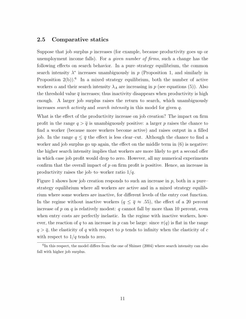
Figure 1 shows how job creation responds to such an increase in p, both in a pure–

strategy equilibrium where all workers are active and in a mixed–strategy equilib-

rium where some workers are inactive, for different levels of the entry cost function.

In the regime without inactive workers (q ≤ q ≈ .55), the effect of a 20 percent

increase of p on q is relatively modest: q cannot fall by more than 10 percent, even

when entry costs are perfectly inelastic. In the regime with inactive workers, how-

ever, the reaction of q to an increase in p can be large: since π(q) is flat in the range

q > q, the elasticity of q with respect to p tends to infinity when the elasticity of c

with respect to 1/q tends to zero.

6In this respect, the model differs from the one of Shimer (2004) where search intensity can also

fall with higher job surplus.

11

pH( )q

pL( )q

q

c q1(1/ )

c q2(1/ )

Figure 1: The response of the worker–firm ratio q to a productivity increase from

pL = 1 to pH = 1.2 with k(λ) = .1 · λ for two exemplary entry cost functions c1

(pure–strategy equilibrium) and c2 (mixed–strategy equilibrium).

2.6 Efficiency

In the model of Albrecht et al. (2006), the decentralized equilibrium is inefficient

along two margins: entry is excessive and workers send too many applications.7 The

first inefficiency also occurs in this model, but the second one must be qualified. In

addition, another inefficiency emerges: it is never socially optimal that a fraction of

workers remains inactive. To obtain these results, consider the problem of a social

planner whose objective is to maximize total surplus per worker net of the costs of

search and entry, with respect to λ and q:

maxλ,q

m(q, λ)p − k(λ) −∫ 1/q

0c(v)dv .

7Albrecht et al. prove the first inefficiency only, but conduct numerical experiments for the

second one.

12

Observe first that the planner’s objective is strictly concave in search intensity λ.

Thus, it is never optimal to let fraction α ∈ (0, 1) of workers search with positive

intensity λA while others are inactive. The planner rather prefers that all workers

search with the same common intensity αλA. Generally, the planner’s objective

depends on a distribution of search intensities, rather than a common intensity as

it is written here. However, it is easy to show that nonparticipation of a fraction

of workers is not optimal.8 The social optimum satisfies the following first–order

conditions:

k′(λ) = e−1−e−λq

q e−λqp ,(8)

c(1/q) = e−1−e−λq

q

[

1 − (1 + λq)e−λq]

p .(9)

Consider first the entry margin for a given common search intensity λ of workers.

In the decentralized equilibrium, the worker–firm ratio equates profit as in (6) to

marginal entry cost c(1/q). On the other hand, the right–hand–side in the optimality

condition (9) is strictly increasing in q and smaller than profit π(q). Hence, the

worker–job ratio q is too small in the decentralized equilibrium; entry is excessive.

The explanation for the inefficiency is a similar “business–stealing effect” as it is

discussed in Albrecht et al. (2006, p. 877): the social benefit of an additional vacancy

falls short of the private benefit since the vacancy can attract workers from other

firms whose vacancies are then left unfilled. Put differently, wages do not internalize

the negative externality that an entrant exerts on incumbents who might lose all

their applicants to the entrant firm. The inefficiency could go away if the wage

for workers with one offer was greater than the monopsony wage (for example, if

there is Nash bargaining with an appropriate choice of worker bargaining power).

Obviously, in the limit λ → ∞ this business–stealing effect disappears and entry

becomes efficient, reconfirming the results of Julien et al. (2000).

Consider now the search intensity margin for a given worker–job ratio q ≤ q. Search

intensity in the decentralized equilibrium is the larger solution to equation (4). The

right–hand–side of the optimality condition (8) is declining in λ. Hence, equilibrium

search intensity λ∗ is too large if and only if the right–hand–side of (4) is smaller

8Proof: in the mixed–strategy equilibrium, net surplus is α[m(αq, λA)p − k(λA)], but if all

workers search with intensity αλA, surplus is m(q, αλA)p − k(αλA). Weak convexity of k implies

αk(λA) ≥ k(αλA), and concavity of 1 − e−x implies that αm(αq, λA) < m(q, αλA).

13

than the right–hand–side of (8) at λ∗ which is the same as

(1 − e−λ∗q)2eλ∗q

λ∗q2 > 1 .

This inequality is true for all values of q > 0 and λ∗ ≥ 1, but it may be violated when

λ∗ < 1 and q is not too large. When all workers send more than one application on

average, search is socially excessive since workers impose a negative externality on

other workers: because firms cannot coordinate their job offers, some workers receive

no offers while others receive multiple offers. This externality is not internalized; on

the contrary, workers desire to receive two or more offers, so the incentive to send a

large number of applications is strong. Indeed, with a linear search cost function, λ∗

is always larger than 1.9 In other situations, however, search intensity can also be

inefficiently low. For instance, with k(λ) = λ2/4, q = 1 and p = 1, the equilibrium

at λ∗ = .38 is smaller than the social optimum at λ = .65.

Proposition 3: A mixed–strategy equilibrium where fraction α ∈ (0, 1) of workers

searches actively with intensity λA is never socially optimal: welfare would increase

if all workers searched with common intensity αλA. A pure–strategy equilibrium

(q∗, λ∗) is not socially optimal since welfare can be raised by increasing q at given

λ∗. Moreover when λ∗ ≥ 1, welfare can be raised by lowering λ at given q∗.

3 Quantitative exploration

3.1 The matching function

I will first demonstrate that this coordination–friction model with a reasonable

choice of the period length and with fixed search intensity is unable to match the em-

pirical response of the job–finding rate with respect to the vacancy–unemployment

ratio. Any linearly homogeneous and concave matching technology gives rise to an

increasing and concave relation between the vacancy–unemployment ratio θ = 1/q

and the job–finding probability ϕ(θ). In my model this relation is given by equation

(2), rewritten as

ϕ(θ) = 1 − e−θ(1−e−λ/θ) .

9This follows from the second–order condition which requires that λz ≥ 1 and hence λ ≥ 1/z >

1.

14

I choose the period length to be one week and set λ to pin down the average weekly

job–finding rate. A short period length is appropriate for this coordination friction

model (as for the others discussed below) since workers send applications only once

in a period and since firms can contact only one worker per period.

Robert Shimer calculates the average monthly job–finding rate in postwar U.S. data

to be around 0.45.10 On a weekly basis, this leads to ϕ = 1 − .551/4.35 ≈ 0.128. As

in Hagedorn and Manovskii (2007), the mean vacancy–unemployment ratio is set

at θ = 0.634 in order to be consistent with Den Haan, Ramey and Watson’s (2000)

estimate of the mean job–filling rate.11 These numbers imply that λ = 0.155. Hence,

an average unemployed worker sends one application within 6.5 weeks and gets a

job after after applying with a chance of z = (1 − e−λq)/(λq) = 88.7%. The first

number seems too small and the second one too large. However, the consideration

of an (irrelevant) mismatch parameter can help explain these magnitudes. Suppose

workers sends λ0 applications on average, and that the firm observes match–specific

productivity after it receives the application. With probability µ the worker fits the

job, but with probability 1 − µ the worker’s productivity is too low for the firm to

be willing to offer the position. Then each worker sends only λ = µλ0 “effective

applications” (those that result in productive matches) which may be much smaller

than the average number of actual applications λ0. Similarly, λq is the average

number of effective applications per vacancy, and z is the offer probability for an

effective application. The actual number of applications and the probability to draw

high match–specific productivity are irrelevant for the quantitative analysis. All that

matters are the effective application rates.

The main result of this analysis is that the elasticity of the matching function is

too low compared to empirical measures. Shimer (2005) estimates the elasticity of

the job–finding rate with respect to the vacancy–unemployment ratio to be 0.28;

Petrongolo and Pissarides (2001) conclude in their survey that the plausible range

for this elasticity is the interval [0.3, 0.5]. With my matching technology and the

empirical values for θ and λ (targeting the average ϕ), I obtain εϕ,θ = .109, clearly

below the range of plausible values.12

10See Shimer (2007b) and http://robert.shimer.googlepages.com/flows11All quantitative results are similar with θ = 0.454 which is obtained from the direct vacancy

measure of the Job Opening and Labor Turnover Survey for the period 12/2007–07/2007.12This result critically depends on the choice of the period length. With a 14–day period, the

elasticity roughly doubles but is still too low. Nonetheless, a short period length is reasonable

15

The result that the elasticity of the matching function is too low is not only true

in my model but in virtually all established coordination–friction models of the

literature. That is, the basic versions of such models, with homogenous agents,

with a reasonable choice of the period length, and without variable search intensity,

are unable to match the empirical elasticity of the matching function. To see this,

consider the matching function of Albrecht, Gautier, and Vroman (2006) which is

general enough to encompass those of most other models as special cases. In their

model, every worker sends a applications, randomly (in equilibrium) to homogenous

firms. After applications arrived, each firm makes a job offer to at most one worker,

rejecting all others. The model gives rise to the job–finding rate

ϕ(θ) = 1 −[

1 − z(a/θ)]a

,(10)

where z(x) = (1 − e−x)/x is the probability to receive an offer. The large–economy

model of Montgomery (1991) and Burdett, Shi, and Wright (2001) is the special case

a = 1, and the model of Julien, Kennes, and King (2000) is the limit a → ∞. For

given a (“fixed search intensity”), this matching function is not flexible enough to

match the job–finding rate at the empirical mean value of θ, since θ is the only free

parameter. However, match–specific productivity enriches the model sufficiently to

achieve this requirement (see also Petrongolo and Pissarides (2001)).13 When the

number of actual applications is a given parameter, match–specific productivity can

be used to target the job–finding rate. As above, suppose firms learn what applicants

are suitable after they receive applications and let µ be the probability that a worker

fits the job. With this modification, the job–finding rate becomes

ϕµ(θ) = 1 −[

1 − µz(aµ/θ)]a

.

When I use the parameter µ to target the weekly job–finding rate at given θ = 0.634,

I find that µ = 0.143 (a = 1), µ = 0.0742 (a = 2), µ = 0.0153 (a = 10); hence the

expected number of effective applications aµ is nearly constant and about the same

as my calibrated value for λ. With fixed search intensity a, the job–finding rate

for this microfoundation of matching frictions. Most newspapers and job agencies publish job

advertisements at weekly or even higher frequency. It seems implausible that job searchers sample

such job openings at a frequency which is much longer than a week.13Alternatively, one could try to use the number of applications a as a free parameter. However,

to match ϕ = 0.124 at θ = 0.639 requires a = .0374, a number which is not compatible with this

model which requires a ∈ IN.

16

responds to little to variations in the vacancy–unemployment ratio. I compute an

elasticity of the job–finding rate with respect to the vacancy–unemployment ratio

of 0.1085 (for a = 1) and 0.1089 (for a = 100), clearly below the range of plausible

values and about the same as with my matching function.

These results suggest that other mechanisms are required in order to match coordination–

friction economies to the data. In the following, I consider a dynamic extension of

the static model in which parameters of a reduced–form search cost function are

calibrated to match the mean and elasticity of the job–finding rate. The purpose of

this study is to answer the following questions.

• How large and how volatile must search costs be to be consistent with the

data?

• What are the implications of variable search intensity for the amplification of

shocks?

• What are the welfare implications?

3.2 The dynamic model

I embed the static model of Section 2 in a dynamic framework in discrete time t. The

environment is stationary, so I consider a steady state equilibrium and confine the

quantitative analysis to comparative statics experiments. Since actual productivity

shocks are quite persistent and since adjustment to the steady state is fast, the

comparative statics response should be a reasonable approximation to the dynamic

response (see also Mortensen (2007)).

Existing jobs end with exogenous probability δ per period. There is no search on

the job, so q is the number of unemployed workers per vacancy. Flow output in

a filled job is p and flow unemployment income is b. This term is interpreted to

encompass unemployment benefits, income from home production, and the utility

value of leisure (in excess of an employed person), but it does not include the cost

of job search. Workers want to maximize their expected utility

E∞∑

t=0

βt[wt − k(λt)] ,

17

where β is the discount factor, wt is wage or unemployment income in period t,

and k(λ) = k · λ1+a/(1 + a) is the utility cost of job search at search intensity λ,

with a ≥ 0 and k > 0. The search cost function is a shortcut to capture both

the opportunity cost of foregone leisure time and the hedonic cost of job search.14

Within every period, unemployed workers and vacant jobs are matched according

to the same process as in the static model. Unmatched agents continue search in

the next period and there is no recall.

I restrict attention to a pure–strategy equilibrium where all nonemployed workers are

active searchers (so they are classified as unemployed in the usual definition). It is

straightforward to characterize mixed–strategy equilibria with inactive workers, but

they do not deliver reasonable predictions in the numerical experiments. Specifically,

in comparison with U.S. data, inactivity (i.e. nonemployed persons who want to work

but do not search) becomes too volatile relative to unemployment, and vacancies

vary too little relative to nonemployment (unemployment plus inactivity). Also the

predictions of the corollary after Proposition 2 are at odds with the evidence. Hence

the inactivity mechanism of this model can only be quantitatively relevant when it

is coupled with substantial heterogeneity.

As in the static model, there are jobs with high and low wages, depending on the

number of offers a worker holds in his hand when leaving unemployment. Although

low–wage earners may have an incentive to search for better–paid jobs, I assume

that employers can identify the current employment status of an applicant and that

employed workers can renegotiate when they obtain better offers later on. Under

these assumptions, employers will never offer their vacant job to an employed worker,

and search on the job does not take place.15

Let V and J j be the values of vacant and filled jobs with wages wj in job status

j = l, h. Suppose that flow costs of a vacant job are c, independent of the number

14An alternative strategy (avoiding a reduced–form search cost function but ignoring hedonic

search costs) would be to include leisure time in the utility function and to calibrate the para-

meters of this function using the empirical Frisch elasticity and time–use data on work and job

search. However, since the functional relationship between the observable “search time” and the

unobservable “search intensity” λ is unclear, I refrained from pursuing this approach.15This assumption is similar as in Julien, Kennes, and King (2006). In their model, however,

low–wage earners search on the job, but only because of between–firm productivity differentials,

which are absent here.

18

of active firms. The Bellman equations are

V = −c + βV + (1 − e−λq)e−λzβ(J l − V ) ,

J l = p − wl + β(1 − δ)J l ,

Jh = p − wh + β(1 − δ)Jh .

In the first equation, firms gain only when they meet an applicant with no other

offer, which happens with probability (1 − e−λq)e−λz. Otherwise they either get no

application or they offer the job to a worker who has at least one other offer. In this

case, Bertrand competition drives the wage wh so high that the value of the filled

job is equal to the value of a vacant job, which is zero, so it follows that wh = p.

The free–entry condition V = 0 is

c = (1 − e−λq)e−λz β(p − wl)1 − β(1 − δ)

.(11)

For workers, let U and Ej be the utility value when the current state is unem-

ployment or employment in a job of status j = l, h. Workers’ Bellman equations

are

U = b + βU + maxλ≥0

[

γ(λz)β(Eh − U) − k(λ)]

,

El = wl + βEl + βδ(U − El) ,

Eh = p + βEh + βδ(U − Eh) .

Here, γ(x) = 1 − (1 + x)e−x is the probability to find a high–wage job (that is, to

obtain two or more job offers) for a worker who receives x = λz offers in expectation.

Since workers with only one offer do not gain at the transition from unemployment

to employment, El = U must hold, which gives rise to the reservation wage equation

wl = b − k(λ) + βγ(λz)(Eh − U) .(12)

The utility increase at a transition into a high–wage job is

Eh − U = p − wl

1 − β(1 − δ).(13)

As in the static model, optimal search intensity equates marginal search costs to the

marginal return from search:

kλa = λz2e−λzβ(Eh − U) .(14)

A steady–state equilibrium is a vector (z∗, λ∗, wl∗, (Eh − U)∗, q∗) solving the five

equations (1), (11), (12), (13), and (14).

19

3.3 Calibration

There are seven parameters (β, δ, a, k, c, b, p) which are calibrated to the U.S. econ-

omy. In comparison with calibration exercises of standard Mortensen–Pissarides

models, the two parameters of the aggregate matching function (a level and an elas-

ticity parameter) are replaced by the two parameters a and k of the reduced–form

search cost function and they play a similar role, targeting the mean and the elas-

ticity of the job–finding rate. Because wages are determined by an ex–post auction,

there is no wage bargaining parameter. Although I could easily augment the model

by Nash bargaining in those matches where a worker has no alternative offers, the

result would be that wages react too much to productivity (see the discussion in 3.4

below).

As above, I specify the period length to be one week. With an annual interest

rate of 5%, this implies β = .9991. With an average weekly job–finding rate of

ϕ = .128 and an average unemployment rate of 5.6%, the weekly separation rate is

fixed at δ = 0.762% which is consistent with Shimer’s (2005) measure of the monthly

separation rate of 2.6% (after adjusting for time aggregation).

Productivity is normalized at p = 1, and vacancy costs are set at Hagedorn and

Manovskii’s (2008) estimated value of c = 0.58, though I do not allow for a pro-

ductivity dependence, as they do. The remaining parameters b, k and a are pinned

down to match the following three targets; the mean job–finding rate of ϕ = 0.128,

the mean vacancy–unemployment ratio θ = 1/q = 0.634, and the elasticity of the

job–finding rate with respect to θ at εϕ,θ = 0.28 (see Section 3.1 for explanations),

provided that variation in the steady–state value of θ is driven by a permanent

productivity shift. In principle, λ (and thus ϕ) reacts to a shock for two reasons:

job surplus Eh −U changes and the job–offer probability z changes. How much job

surplus changes relative to z depends of course on the source of the shock. However,

εϕ,θ does not change much when variation in θ is driven by shocks to the separa-

tion rate or to unemployment income. More precisely, when parameter a targets

εϕ,θ = 0.28 for a p shock, it can be verified that then εϕ,θ = 0.2804 (with a b shock)

and εϕ,θ = 0.2803 (with a δ shock).

The calibration targets imply that b = 0.955, k = 6051.6 and a = 5.27.16 As in

16Numerically, for given a and the targets for ϕ and θ (and hence λ and z), equation (11) yields

wl, k follows from (13) and (14) and b follows from (12). Then a is adjusted to target εϕ,θ.

20

Section 3.1, mean search intensity is at λ = 0.155 and the chance to obtain an offer

is z = 0.887. Mean search costs are modest at k(λ) = 0.0081, so that the flow utility

from unemployment is at b = b − k(λ) = 0.947.

The reservation wage is at wl = 0.9738, so that the mean wage is at w = αwl+1−α =

0.9756, where α = λze−λz/(1 − e−λz) = 0.933 is the share of workers in low–wage

jobs. Finally, because of a > 1 and Proposition 1, the first–order condition (14)

indeed characterizes the unique equilibrium in pure strategies. Table 1 summarizes

parameter choices and their explanation.

Parameter Value Explanation

β 0.9991 Annual interest rate 5%

δ 0.00762 Unemployment rate u = 5.6%

p 1 Normalization

c 0.58 Hagedorn and Manovskii (2008)

k 6051.6 Job–finding rate ϕ = 0.128 (via λ)

b 0.955 Vacancy–unemployment ratio θ = 0.634 (via wl and J l)

a 5.27 Matching–function elasticity εϕ,θ = 0.28

Table 1: Parameter choices.

3.4 Quantitative implications

How does the economy respond to a permanent unanticipated productivity increase?

As implied by Proposition 1, search intensity will go up. Indeed, at the calibrated

parameter values, I calculate elasticities ελ,p = 4.7 and εk(λ),p = 29.7. Although

search costs are small (only 0.8% of unemployment utility), they are quite volatile,

varying between 0.3% and 1.3% when p varies between 0.98 and 1.02. Empirical

results on the response of search intensity to market conditions are inconclusive. The

findings of Shimer (2004) do not support procyclical search intensity. He considers

CPS data and uses two measures of search intensity. One is the “probability to

search” which is irrelevant here since nonparticipation is not considered. The other

is the “number of job search methods”. However, the variability of this measure

is small and it is unclear how this number correlates with application rates and

with search time, which are relevant here. On the other hand, Krueger and Mueller

21

(2008) examine time–use data and find that job–search time responds positively to

labor market conditions. Using cross–state variation in unemployment benefits, they

calculate an elasticity of job search with respect to benefits of around -2. My model

yields the elasticity ελ,b0 = −1.4, where b0 = .28 = .29w is a plausible value for the

level of unemployment benefits.17 If search intensity λ is proportional to job–search

time, this finding suggests that my calibration does not overstate the responsiveness

of search intensity to labor market conditions. Krueger and Mueller also find that

an individual’s predicted wage has a strong quantitative impact on job–search time.

It is unsurprising that the model’s response of the vacancy–unemployment ratio to

a productivity shock is of the same magnitude as in the data. In fact, my level of

flow unemployment income is about the same as in the calibration of Hagedorn and

Manovskii (2007) which is well known to yield a strong amplification. This is even

true when search intensity is fixed at the steady–state value, in which case I find that

ελ fixedθ,p = 18.8, about 10 times as large as in Shimer’s (2005) calibration of the search

and matching model where flow unemployment income is at b = 0.4. When search

intensity varies positively with productivity, the amplification of productivity is even

stronger since the job–finding rate increases and hence unemployment decreases

further. However, the impact on the elasticity is modest; it merely increases to

ελ variableθ,p = 22.9, so the order of magnitude does not change. My calibration also

gives rise to a reasonable response of wages. I calculate an elasticity of the mean

wage with respect to productivity of εw,p = 0.61. This number is a bit larger than the

estimate of εw,p = 0.45 used by Hagedorn and Manovskii to pin down the bargaining

power parameter in the Mortensen–Pissarides model. Again, this is not surprising.

In their calibration, workers get 5.2% of job surplus, whereas here 6.7% of workers

obtain the full job surplus whilst the rest works at the reservation wage, obtaining

zero surplus. Therefore the wage response in my model is somewhat stronger, and

this is the reason why it makes little sense to augment the model by Nash bargaining

in one–one matches.

It is instructive to see what happens when the level of unemployment utility is

reduced to the value used by Shimer (2005) in his calibration of the search–and–

matching model. To this end, I choose b to obtain in steady state b = b−k(λ) = 0.4.

In the absence of a Nash bargaining parameter, it is clear that this choice blows up

profits, so I set now c = 6.61 to still target the steady–state vacancy–unemployment

17See Nickell, Nunziata, and Ochel (2005) who calculate a replacement ratio for the U.S. of 29%.

22

ratio at θ = 0.634. Again a is chosen to target εϕ,θ = 0.28, and k is chosen to

target ϕ = 0.128. Interestingly, the elasticity of search costs a = 5.27 is the same

as before, but k is about one order of magnitude larger. Hence I find that search

costs are k(λ) = .092, now more than 20% of unemployment utility. On the other

hand, the responsiveness of search intensity (and search costs) are reduced by an

order of magnitude; that is ελ,p = 0.416. As with the original parameter values,

variable search intensity raises the responsiveness of the vacancy–unemployment

ratio only slightly. Specifically, εθ,p increases from 1.65 with fixed intensity to 2.01

with variable search intensity.

3.5 Welfare

Results from section 2.6. show that equilibrium is not efficient in general: entry

is excessive and search intensity can be too high or too low. The dynamic model

requires a separate analysis of the welfare issue. One important adjustment concerns

the role of unemployment benefits which are pure transfers and do not contribute to

welfare.18 However, benefits induce a wedge between the private and the social job

surplus, which dampens the incentives to search for workers and firms. This effect

counteracts my previous findings that entry is excessive and that search intensity is

excessive when λ > 1.

Because of quasilinear preferences, the planner’s objective is to maximize a utili-

tarian welfare function which adds up the discounted value of the income stream

net of entry cost and worker’s search effort costs. The recursive formulation of this

problem is

W (u) = maxλ,q

{

u · [b − k(λ)] + (1 − u) · p − cuq + βW (u′)

s.t. u′ = u + δ(1 − u) − m(q, λ)u

}

.(15)

Here u is the unemployment rate (the only state variable), W (u) is welfare when

current unemployment is u, m(q, λ) is the matching function (2), and b = b − b0 is

18Of course, matters would be different if workers were risk averse and markets were incomplete.

In their welfare analysis, Hagedorn and Manovskii (2008) correct for distortionary taxes, but they

ignore any positive role of government.

23

flow unemployment utility net of benefits b0 and gross of search costs. I obtain the

following characterization of the social optimum.

Proposition 4: In the social optimum, the unemployment–vacancy ratio q and

search intensity λ are independent of the state variable u and satisfy the first–order

conditions

c = βe−λz[1 − (1 + λq)e−λq]S ,(16)

k′(λ) = βe−λze−λqS ,(17)

where z = (1 − e−λq)/(λq) and

S =p − b + k(λ)

1 + βδ − βe−λz(1 + λz) + βλe−λze−λq

is the social value of an employed person.

Proof: Appendix.

The intuition behind the optimality conditions is easy to explain. In (16), the term

e−λz[1−(1+λq)e−λq] is the same as d[m(q, λ)]/d[1/q], i.e. the number of new matches

of an additional vacancy. Hence the term on the right–hand side is the social return

of a vacancy which must be equal to marginal cost on the left–hand side. Similarly

in (17), the term e−λze−λq is the same as d[m(q, λ)]/d[λ], so the right–hand side is

the marginal social return of an additional unit of search intensity.

When there are no unemployment benefits, it is straightforward to show that entry

is excessive. Indeed, the free–entry condition (11), using (12) and (13), can be

expressed as

c = βe−λz(1 − e−λq)p − b + k(λ)

1 + βδ − βe−λz(1 + λz).(18)

It follows immediately that the right–hand side of (16) is smaller than the right–

hand side of (18), at the same values of λ and q when b = b. Since the right–hand

side of (16) is increasing in q, the equilibrium level of q is smaller than the socially

optimal level of q (at given λ). Hence, for any given level of search intensity, there

is too much entry. Obviously, this result can change when benefits b − b > 0 are

large enough.

Table 2 compares the equilibrium at the benchmark calibration with the social

optimum, where I set benefits to b0 = .28, at 29% of the mean wage (see footnote 17).

24

Compared with the social optimum, equilibrium search intensity is about 25 percent

too low, and the vacancy–unemployment ratio 1/q is more than twice as large. The

planner would choose about the same unemployment rate, but the optimal vacancy

rate would be about half of what is in the data. Nonetheless, total welfare W (u) is

only about 1% below optimum. The last three columns of the table show the three

components of flow surplus: output, flow utility of the unemployed, and vacancy

costs. The planner would like to reduce unemployment utility slightly (by inducing

them to search more) and create fewer vacancies; actual output (employment) would

increase only minimally.

λ q u(%) Welfare Flow Flow utility of Vacancy

output unemployed costs

Equilibrium 0.155 1.577 5.6 1063.7 0.944 0.037 0.021

Social opt. 0.207 3.712 5.36 1075.6 0.946 0.033 0.008

Table 2: Equilibrium versus social optimum.

4 Conclusion

This paper develops a model of coordination frictions with variable search inten-

sity in which equilibrium can be fully characterized by a simple set of first–order

conditions. Under bad labor market conditions, there can be an equilibrium where

only a fraction of workers are active searchers whilst the rest stays out of the labor

market. This inactivity phenomenon is not socially desirable; the planner desires

that all homogenous workers search with a common intensity. But even under better

labor market conditions, equilibrium is typically inefficient, as there are too many

vacancies and a suboptimal level of search intensity. In the quantitative part of this

paper, I argue that variable search intensity helps to improve the fit of coordination–

friction models which typically have a too low matching–function elasticity, and I

examine the comparative statics features of a reasonably calibrated dynamic model.

Of course, variable search intensity may not be the only mechanism raising the

responsiveness of the job–finding rate. Lester (2008) shows that an endogenous ca-

pacity choice in the model of Burdett, Shi and Wright (2001) can also raise the

elasticity of the job–finding rate with respect to productivity.

25

The following two extensions are left for future work. The first is the effect of

heterogeneity on search intensities. On the one hand, when there are jobs with

high and low productivities, it is interesting to know whether workers search too

hard for the good jobs and too little for the bad ones, and how much they diversify

their “search portfolio”. A similar issue is analyzed in Gautier and Wolthoff (2007).

On the other hand, when workers are endowed with different skills, it should be

understood how much search intensities between skill groups differ, and what the

implications are for skill differences in wages and employment rates.

Another variation concerns the wage determination mechanism. If firms commit to

posted wages and workers apply after sampling these postings, there should be wage

dispersion similarly as in the model of Burdett and Judd (1983). Such a model can

also be examined when firms are able to recall all their applicants as in Kircher’s

(2007) model.

Appendix

Proof of Proposition 1:

Consider the best response problem of a particular worker deciding search intensity

λ when all others search with intensity λ0. Let z = z(λ0) = [1− e−λ0q]/(λ0q) be the

chance to receive an offer when applying. The worker’s best response is the solution

to U ′z(λ) = 0 which is

z2e−λz pk = λa−1 .(19)

Because of a > 1, this equation has a unique solution which is the global maximum

of Uz(.). Hence, for any λ0 there is a unique best response, denoted λ = S(z(λ0)) ≡

R(λ0). Moreover, because of z(0) = 1 and z(∞) = 0, R(0) > 0 and R(∞) = 0.

Since R is continuous, a Nash equilibrium λ = R(λ) > 0 exists.

To prove uniqueness, it suffices to show that R′(λ) = S ′[z(λ)]z′(λ) < 1 at any

λ = R(λ). One has

z′(λ) = −1 − e−λq(1 + λq)

λ2q,

and implicit differentiation of (19) yields

S ′(z) =λ(2 − λz)

λz2 + (a − 1)z.

26

Combining these two shows that R′(λ) < 1 (at any λ = R(λ)) is equivalent to

−(2 − λz)[1 − e−λq(1 + λq)]

[λz2 + (a − 1)z]λq< 1 .(20)

With a > 1, a sufficient condition for this inequality is that

−(2 − λz)[1 − e−λq(1 + λq)] < z2λ2q .

Substitution of z = (1 − e−λq)/(λq) obtains the equivalent

2eλq − 2 − 2λq > λe−λq − λ .

This inequality is satisfied since the right–hand side is negative and since ex > 1+x.

Lastly, the unique Nash equilibrium λ∗ increases in p/k because the best–response

curve R(.) shifts upwards when p/k increases, which follows immediately from (19)

defining λ = S(z). 2

Proof of Proposition 2:

Consider again the best–response problem of a particular worker when λ0 is the

average search intensity of other workers (who either all search with intensity λ0,

or fraction α search with intensity λA = λ0/α). As in the proof of Proposition

1, z = z(λ0) is the job–offer probability conditional on applying. The worker’s

objective function Uz(λ) has an interior local maximum whenever the increasing,

strictly concave λa has two positive intersections with the hump–shaped λz2e−λzp/k.

Such intersections exist if and only if

pk > e1−a(1 − a)a−1z−1−a .

This is the same as

z = z(λ0) > z ≡[

ke1−a

p(1 − a)1−a

]1/(1+a),

which is the same as

λ0 < λ0 ≡1qΦ(z) .

Therefore, for any λ0 < λ0, Uz(λ) has an interior local maximum, to be denoted

λ = R(λ0) > 0. Worker payoff at the local maximum is then

Uz(λ) = p[

1 − e−λz(1 + λz)]

− k1 + aλ1+a

= pe−λz[

eλz − 1 − λz −(λz)2

1 + a

]

.

27

Therefore, λ = R(λ0) is a global maximum (that is, Uz(λ) ≥ 0 so that a deviation

to λ = 0 does not raise payoff) if and only if

λz ≥ x ,(21)

where x is the unique positive solution of

ex = 1 + x + x2

1 + a .

Since λ = R(λ0) solves λa = λz2e−λzp/k,

eλz

(λz)1−akp = z1+a

holds. Because eλz/(λz)1−a is increasing in λz ≥ 1 − a (where λz > 1 − a follows

from the second–order condition U′′

z (λ) < 0), condition (21) is equivalent to

ex

x1−akp ≤ z1+a ,

or

z = z(λ0) ≥ z ≡[

kex

px1−a

]1/(1+a).

Therefore, λ = R(λ0) > 0 is best response to λ0 iff

λ0 ≤ λ0 ≡1qΦ(z) ,

and it is the unique best response if the inequality is strict. Note also that λ0 > λ0.

Further, for any λ0 ≥ λ0, λ = 0 is best response to λ0, and it is the unique best

response when the inequality is strict.

Since λ0 ≤ 0 is equivalent to z ≥ 1, λ = 0 is the unique Nash equilibrium when p ≤

kex/x1−a (part (c) of the Proposition). When p > kex/x1−a is satisfied, λ0 > 0 holds.

In that case, a pure–strategy equilibrium exists when R(λ0) ≤ λ0 (in which case the

best response curve R(λ0) crosses the 45–degree line at some λ0 ≤ λ0), whereas a

mixed–strategy equilibrium exists when this inequality is reversed (in which case

the 45–degree line is “crossed” as the best response correspondence jumps at λ0).

By definition of λ0 and z, the sufficient condition for a pure–strategy equilibrium is

R(λ0) = xz ≤ λ0 = 1

qΦ(z) ,

which is the same as

q ≤ q ≡zΦ(z)

x .

28

This condition is not only sufficient but also necessary for a pure–strategy equilib-

rium provided that R′(λ) < 1 holds at any λ = R(λ) (so that the 45–degree line can

be crossed at most once). This condition then also implies that the Nash equilibrium

is unique. As in the proof of Proposition 1, R′(λ) < 1 holds at any λ = R(λ) if

condition (20) holds. The denominator on the left–hand side is positive because of

the second–order condition λz > 1 − a. Hence, the inequality is

−(2 − λz)[1 − e−λq(1 + λq)] < λq[λz2 + (a − 1)z] .

Substitution of z = (1 − e−λq)/(λq) yields

2λq < λ(1 − e−λq) + (1 + a)(eλq − 1) .

Again because of the second–order condition λ ≥ (1− a)/z = (1− a)λq/(1− e−λq),

a sufficient condition for this inequality is that

2λq < (1 − a)λq + (1 + a)(eλq − 1) .

This is the same as

0 < (eλq − 1 − λq)(1 + a) ,

which is obviously true for any λ > 0. 2

Proof of Proposition 4:

As in section 7.2 of Rogerson, Shimer, and Wright (2005), it is straigtforward to

show that W (.) is affine–linear; it takes the form W (u) = w0 − S · u where S is

marginal social value of an employed worker. Differentiation of (15) with respect to

u together with the envelope theorem yields

S = p − b + k(λ) + c/q + βS(e−λz − δ) .(22)

The first–order conditions for λ and q are

k′(λ) = βe−λze−λqS ,(23)

c = βe−λz[1 − (1 + λq)e−λq]S .(24)

These conditions confirm that optimal λ and q do not depend on the state variable

u, so W (.) is indeed affine–linear. Both first–order conditions are the same as in

Proposition 4. The value S follows after substitution of (24) into (22) and solving

for S. 2

29

References

Acemoglu, D. (2001): “Good Jobs versus Bad Jobs,” Journal of Labor Economics,

19, 1–22.

Albrecht, J., P. Gautier, and S. Vroman (2006): “Equilibrium Directed

Search with Multiple Applications,” Review of Economic Studies, 73, 869–891.

Albrecht, J., and S. Vroman (2002): “A Matching Model with Endogenous

Skill Requirements,” International Economic Review, 43, 283–305.

Burdett, K., and Judd (1983): “Equilibrium Price Dispersion,” Econometrica,

51, 955–969.

Burdett, K., S. Shi, and R. Wright (2001): “Pricing and Matching with

Frictions,” Journal of Political Economy, 109, 1060–1085.

Butters, G. (1977): “Equilibrium Distribution of Sales and Advertising Prices,”

Review of Economic Studies, 44, 465–491.

Den Haan, W., G. Ramey, and J. Watson (2000): “Job Destruction and

Propagation of Shocks,” American Economic Review, 90, 482–498.

Galenianos, M., and P. Kircher (2008): “Directed Search with Multiple Job

Applications,” forthcoming in Journal of Economic Theory.

Gautier, P., and R. Wolthoff (2007): “Simultaneous Search with Heteroge-

neous Firms and Ex Post Competition,” CEPR Discussion Paper 6169.

Hagedorn, M., and I. Manovskii (2007): “The Cyclical Behavior of Equilibrium

Unemployment and Vacancies Revisited,” forthcoming in American Economic

Review.

Hall, R. (1977): “An Aspect of the Economic Role of Unemployment,” in Mi-

croeconomic Foundations of Macroeconomics, ed. by G. Harcourt. Macmillan,

London.

Julien, B., J. Kennes, and I. King (2000): “Bidding for Labor,” Review of

Economic Dynamics, 3, 619–649.

30

(2006): “Residual Wage Disparity and Coordination Unemployment,” In-

ternational Economic Review, 47, 961–989.

Kircher, P. (2007): “Efficiency of Simultaneous Search,” Working Paper, Univer-

sity of Pennsylvania.

Krueger, A., and A. Mueller (2008): “Job Search and Unemployment Insur-

ance: New Evidence from Time Use Data,” IZA Discussion Paper No. 3667.

Lagos, R. (2000): “An Alternative Approach to Search Frictions,” Journal of

Political Economy, 108, 851–873.

Lester, B. (2008): “Directed Search with Multiple Vacancies,” Working Paper,

University of Western Ontario.

Montgomery, J. (1991): “Equilibrium Wage Dispersion and Interindustry Wage

Differentials,” Quarterly Journal of Economics, 106, 163–179.

Mortensen, D. (2007): “Island Matching,” NBER Working Paper 13287.

Nickell, S., L. Nunziata, and W. Ochel (2005): “Unemployment in the OECD

since the 1960s: What Do We Know?,” The Economic Journal, 115, 1–27.

Petrongolo, B., and C. Pissarides (2001): “Looking into the Black Box: A

Survey of the Matching Function,” Journal of Economic Literature, 39, 390–431.

Pissarides, C. (2000): Equilibrium Unemployment Theory. The MIT Press, Cam-

bridge, MA, 2 edn.

Rogerson, R., R. Shimer, and R. Wright (2005): “Search–Theoretic Models

of the Labor Market: a Survey,” Journal of Economic Literature, 43, 958–988.

Shimer, R. (2004): “Search Intensity,” Working Paper, University of Chicago.

(2005): “The Cyclical Behavior of Equilibrium Unemployment and Vacan-

cies,” American Economic Review, 95, 25–49.

(2007): “Mismatch,” American Economic Review, 97, 1074–1101.

31