Climatic ChangeDOI 10.1007/s10584-011-0049-1

Variability of African farming systemsfrom phenological analysis of NDVI time series

Anton Vrieling · Kirsten M. de Beurs · Molly E. Brown

Received: 6 May 2009 / Accepted: 27 January 2011© The Author(s) 2011. This article is published with open access at Springerlink.com

Abstract Food security exists when people have access to sufficient, safe and nutri-tious food at all times to meet their dietary needs. The natural resource base is one ofthe many factors affecting food security. Its variability and decline creates problemsfor local food production. In this study we characterize for sub-Saharan Africavegetation phenology and assess variability and trends of phenological indicatorsbased on NDVI time series from 1982 to 2006. We focus on cumulated NDVI overthe season (cumNDVI) which is a proxy for net primary productivity. Results areaggregated at the level of major farming systems, while determining also spatialvariability within farming systems. High temporal variability of cumNDVI occurs insemiarid and subhumid regions. The results show a large area of positive cumNDVItrends between Senegal and South Sudan. These correspond to positive CRU rainfalltrends found and relate to recovery after the 1980’s droughts. We find significantnegative cumNDVI trends near the south-coast of West Africa (Guinea coast) andin Tanzania. For each farming system, causes of change and variability are discussedbased on available literature (Appendix A). Although food security comprises morethan the local natural resource base, our results can perform an input for food secu-rity analysis by identifying zones of high variability or downward trends. Farming

Part of the work was done while A. Vrieling worked at the Joint Research Centre of theEuropean Commission in Ispra (VA), Italy.

A. Vrieling (B)Faculty of Geo-Information Science and Earth Observation (ITC), University of Twente,P.O. Box 217, 7500 AE Enschede, The Netherlandse-mail: a.vrieling@utwente.nl

K. M. de BeursDepartment of Geography, University of Oklahoma, 100E. Boyd Street, SEC Suite 684,Norman, OK 73019, USA

M. E. BrownBiospheric Sciences Branch, NASA Goddard Space Flight Center, Greenbelt,MD 20771, USA

https://ntrs.nasa.gov/search.jsp?R=20110015377 2020-02-18T11:06:35+00:00Z

Climatic Change

systems are found to be a useful level of analysis. Diversity and trends found withinfarming system boundaries underline that farming systems are dynamic.

1 Introduction

Local agricultural production is a key element of food security in many Africancountries (Alexandratos 1999). Despite globalization and food trade, access to foodremains a major problem for an important part of the population of sub-SaharanAfrica (SSA). Organizations that monitor food security in Africa often use satelliteremote sensing as a key indicator of variation in food production (Brown 2008). Thenormalized difference vegetation index (NDVI) as derived from coarse-scale satelliteimagery is often used because it provides observations at a daily time step, allowingfor frequent updating of the vegetation status. NDVI is defined as the differencebetween the near-infrared and red reflections divided by the sum of the two (Tucker1979). Although NDVI is affected by soil background, atmospheric scattering, and isrelatively insensitive to high biomass levels, it provides sufficient stability to captureseasonal and inter-annual changes in vegetation status (Huete et al. 2002). Organi-zations like the European Joint Research Centre (JRC), the United State’s FamineEarly Warning System Network (FEWS-NET), and the United Nations Food andAgriculture Organization (FAO) use NDVI time series for early warning of po-tential food production problems in African countries (e.g. Rojas et al. 2005).

The vigor and development of vegetation depends on available natural resources.For the African continent particularly water and nutrient availability are limitingfactors. Vegetation development can be studied by looking at its phenologicalcharacteristics including germination, leaf emergence, and start of senescence. Landsurface phenology is defined as the spatio-temporal development of the vegetatedland surface as observed by synoptic satellite sensors (de Beurs and Henebry 2005a).At an aggregated level, NDVI time series from satellite data can approximatephenological stages and thus characterize the general vegetation behaviour withinits spatial footprint (Justice et al. 1985; Reed et al. 1994). NDVI-derived measurescharacterizing the vegetation’s temporal behavior are referred to as phenologicalmetrics. Phenological metrics have also been used to assess food production (Funkand Budde 2009). A phenological metric of special interest is the seasonally cumu-lated NDVI (cumNDVI) as it is related to net primary productivity (NPP: Awayaet al. 2004; Lo Seen Chong et al. 1993).

The Advanced Very High Resolution Radiometer (AVHRR) provides the long-est NDVI record with global coverage (Tucker et al. 2005). Using the AVHRRinstrument on multiple satellites since 1981, the resulting 26-year vegetation datarecord permits the examination of variability between years as well as trends(de Beurs and Henebry 2005b). In relation to farming systems trends and variabilityin NDVI records can give information on the stability of the natural resource base ofthe system. For example, areas experiencing frequent droughts will likely show highvariability in one or more phenological metrics. For Africa, AVHRR time series havebeen used extensively for trend analysis (e.g. Fuller 1998; Herrmann et al. 2005),but to a more limited extent in relation to phenology. An exception is Heumannet al. (2007) who found positive cumNDVI trends in 250–1100 mm rainfall regionsof West-Africa for 1982–2005, but did not analyze areas outside the 4◦–18◦N range.

Climatic Change

Tateishi and Ebata (2004) found similar positive cumNDVI trends for the 1982–2000period.

Dixon et al. (2001) classified 72 global farming systems (GFS) in six developingregions worldwide. They define farm systems as the household, its resources, andthe resource flows and interactions at the individual farm level. A farming system isdefined as a group of individual farm systems that broadly contain a similar resourcebase, enterprise patterns, household livelihoods and constraints. The main goal oftheir work was to provide a framework within which agricultural development strate-gies may be determined. Their classification was based on the available natural re-source base and the dominant pattern of farm activities and household livelihoods.

The purpose of this study is to characterize nine of the farming systems (FS)identified in sub-Saharan Africa with respect to land surface phenology as measuredby the AVHRR record. Based on a consistent processing for the period 1982–2005 wedetermine phenological variability and trends. The main focus is on cumNDVI. Weaggregate our results from 8-km pixels to farming system polygons. Because Dixonet al. (2001) stress that sharp boundaries between neighboring farming systems donot occur, we first subdivide the polygons to encompass spatial variability within eachsystem. Although the study deals with farming systems we choose to not specificallyfocus on agricultural areas only, but to evaluate the total natural resource base ofeach system. A consequence of that choice is that observed trends cannot merelybe attributed to changes in vegetation phenology, but also to land cover conversions(Brink and Eva 2009). Hence, we show where consistent trends occur which indicatea change in the natural resource base. Potential drivers of change are identified basedon literature and we compare our phenology results with rainfall and temperaturetrends for the same time period. We discuss possible implications for food security.

2 Materials and methods

2.1 Farming systems

The farming systems map for SSA was taken from Dixon et al. (2001). In this studywe address only the agricultural FS that are predominantly rainfed, as shown in Fig. 1.Consequently, the arid, pastoral, irrigated, and urban classes were not considered.Additionally the forest based system was discarded, because limited intra-annualNDVI variability and the dominant shifting cultivation practices prevent effectivephenological characterization. This leaves nine farming systems, which we order asin Dixon et al. (2001). The farming systems and their principal crops and livestockare listed below:

– Tree crop (TC): cocoa, coffee, oil palm, rubber, yams, maize;– Rice-tree crop (RT): rice, banana, coffee, maize, cassava, legumes, livestock;– Highland perennial (HP): banana, plantain, enset, coffee, cassava, sweet potato,

beans, cereals, livestock, poultry;– Highland temperature mixed (HT): wheat, barley, teff, peas, lentils, broadbeans,

rape, potatoes, sheep, goats, livestock, poultry;– Root crop (RC): yams, cassava, legumes;– Cereal-root crop mixed (CR): maize, sorghum, millet, cassava, yams, legumes;– Maize mixed (MM): maize, tobacco, cotton, cattle, goats, poultry;

Climatic Change

– Large commercial and smallholder (LC): maize, pulses, sunflower, cattle, sheep,goats;

– Agro-pastoral millet/sorghum (AP): sorghum, pearl millet, pulses, sesame, cattle,sheep, goats, poultry;

Dixon et al. (2001) provide a more detailed description of the FS and their charac-teristics. We use the two-letter codes above to refer to the systems.

Individual FS polygons often cover large areas. To address spatial variabilitywithin farming systems we combine the FS map with sub-national administrativelayers. For this the first sub-national administrative units of FAO’s GAUL (GlobalAdministrative Unit Layers) database were used. Due to different political organi-zation per country, the size of individual units may greatly vary. To obtain a fairlyhomogeneous unit size, a combination of the FS map and GAUL was performed inthe following way. First, FS polygons of less than 40,000 km2 were conserved in theirpresent form and not subdivided. Second, an intersection was performed between theremaining FS and GAUL polygons. Third, iteratively for resulting polygons smallerthan 20,000 km2 the smallest polygon was merged with the smallest neighboringpolygon having the same FS and preferentially falling within the same country. Ifno neighboring polygon of the same FS was present in the same country, polygons ofdifferent countries were merged. The final result is the same FS map but with a sub-division of large FS units (the grey lines in Fig. 1). The area threshold values were setin such a way that each polygon contained sufficient NDVI pixels for effective aggre-gation (see Section 2.2).

2.2 NDVI data and phenology extraction

We used the AVHRR NDVI dataset from the NASA Global Inventory Monitoringand Modeling Systems (GIMMS) group at the Laboratory for Terrestrial Physics

Fig. 1 Global farming systemsof sub-Saharan Africaaddressed in this article (afterDixon et al. 2001). The thingrey lines delimit the sub-unitsused in our analysis. In mostcases country borders (blacklines) are respected, but asub-unit may occasionally spantwo countries

Climatic Change

(Tucker et al. 2005). The dataset contains 15-day maximum value NDVI compositesat 8-km resolution for July 1981 to December 2006. It is based on six NOAA(National Oceanic and Atmospheric Administration) satellites. SPOT VegetationNDVI is used for intercalibration between NOAA-14 and NOAA-16 and -17. Thedataset is corrected for factors not relating to vegetation, although some data prob-lems remain in the current version (Pinzón et al. 2005). Due to AVHRR’s widespectral bands the presence of water vapor in the atmosphere lowers NDVI values,although maximum-value compositing reduces this effect (Brown et al. 2008). Toremove residual cloud contamination, we applied the iterative Savitzky-Golay algo-rithm (Savitzky and Golay 1964) as described by Chen et al. (2004). NDVI-valuesbelow 0 and rises of more than 0.30 NDVI units in 15 days were masked out beforeapplying the filter. All subsequent analysis was based on the Savitzky-Golay filtereddata.

Several methods exist for extracting phenology from satellite data, but field-basedvalidation efforts are still limited (Reed et al. 2009). In North America ground-measured plant phenology was compared with 10 extraction methods (White et al.2009). The comparison showed that the start of the season was generally wellrepresented by the variable threshold method of White et al. (1997) and a harmonicanalysis model based on the Fourier-transformation by Roerink et al. (2000). For theWest African Sahel, Brown and de Beurs (2008) compared a quadratic method withground measured sowing dates and obtained good results. However, the quadraticmethod may be less robust for other environments (White et al. 2009) and bimodalseasons. We selected the variable threshold method White et al. (1997) to extractphenology from the NDVI time series. This method determines per year and perpixel the annual maximum and minimum NDVI. The average between both is takenas the threshold. Onset and offset of the season are the points where the NDVIprofile passes the threshold value in upward and downward direction respectively.We call these points start of season (SOS) and end of season (EOS).

Phenology extraction for the entire SSA is somewhat complex since seasonsspan different calendar years and double seasons occur. To limit strong artificialphenology fluctuations between years, we extended White’s method with a searchingalgorithm. First, a long term average NDVI-profile was constructed per pixel (i.e. theNDVI climatology). Based on this profile the occurrence of maxima and minima wasdocumented. A maximum for a pixel is the point where it has a) the highest value ina window ranging from three values before and three values after, and b) is higherthan the average value of absolute maximum and minimum for that pixel. For theminimum a similar logic was applied. Two seasons occur for a pixel if two maxima andtwo minima separate each other. Based on the NDVI climatology per pixel and itscorresponding maxima and minima, we then extract phenology from the yearly data.For that purpose, we search per season and pixel the SOS in the range of three valuesbefore minimum and three values after corresponding maximum. This procedure isillustrated in Fig. 2. EOS is then the first moment after the yearly maximum wherethe profile attains the threshold value. The values of SOS and EOS are interpolatedbetween different 15-day periods, if needed.

We discarded arid areas, dense forests, and areas with limited intra-annual vege-tation variability by masking pixels that had an average NDVI outside the range 0.2–0.7 or a coefficient of variation of less than 0.1. To avoid problems of seasons span-ning different calendar years, we always assessed two years at a time. This resulted

Climatic Change

Fig. 2 Illustration of searching algorithm to extract phenology. For the NDVI climatology themaximum and minimum are determined. Then for individual years the maximum is determinedwithin a temporal search window (three periods before and after). Subsequently we find the firstpreceding minimum, which should be between three periods before average minimum and the yearmaximum. Finally, we find SOS where the NDVI profile reaches the 50%-value between yearlymaximum and minimum

for each pixel in a time series of phenology metrics, ranging from 1982 to 2005. Themetrics extracted and used in further analysis are SOS, length of season (LOS),maximum NDVI value (maxNDVI), and cumulated NDVI over the season (cum-NDVI). These are illustrated in Fig. 3 and are the same as in Brown et al. (2010). Theextraction of the additional metrics is straightforward based on SOS, EOS, and thefiltered time series. LOS is the difference between EOS and SOS. We defined thatLOS should be at least more than a month to be valid, and before calculating othermetrics. If present, the metrics were also calculated for the second season. For thepurpose of the analysis described here, we combined the cycles for LOS, maxNDVI,cumNDVI. If two cycles are present, per pixel we take LOS as the sum of the twoLOS values for cycle 1 and 2. The same was done for cumNDVI, while for maxNDVIthe maximum value of both cycles was taken.

Fig. 3 Phenology metricsaddressed in this article, i.e.start of season (SOS), end ofseason (EOS), length ofseason (LOS), maximumNDVI value (maxNDVI), andcumulated NDVI over theseason (cumNDVI)

Climatic Change

The phenology metrics were aggregated 1) per farming system divided in northand south of the equator, and 2) for the polygons defined in Section 2.1. Suchaggregation could be done based on a crop mask to focus on agricultural areasonly. Vrieling et al. (2008) combined AfriCover (http://www.africover.org/), FAOcrop zones, and GLC2000 (Global Land Cover: Bartholomé and Belward 2005) toobtain an optimal crop mask for Africa, and aggregated phenology based on thismask. More sources for crop masks exist (e.g. Bicheron et al. 2008; Biradar et al.2009; Friedl et al. 2002; Ramankutty et al. 2008). However, datasets show strongdiscrepancies between them (Fritz and See 2008) while many products contain alarge number of mosaic classes (Bicheron et al. 2008). Our experience learns thatfor areas erroneously omitted as crops no aggregated phenology results could beobtained, or aggregated values were only based on a very limited number of pixels.Our choice for not using a crop mask in this study is based on the following reasons: 1)we choose to evaluate the total natural resource base of the farming systems (see alsoSection 1), 2) an accurate well-validated crop mask does not exist for the region whileusing a mask of limited or unknown accuracy can strongly bias our results, and 3)crop distribution changes over time which is not accounted for in existing stationarycrop masks. Averaging the derived metrics (i.e. pixels) inside a polygon thus givesus per year the phenology metrics for the average resource base. To obtain a validrepresentative value for a specific polygon and year, at least 25 pixels with validphenology metrics should be present. A second season was only documented for SOSif the number of pixels with valid phenology metrics for the second season were atleast 50% of pixels for the first season. Hence below 50% a second season was judgednot representative for the polygon.

2.3 Variability and trend calculation

Summary statistics per farming system were derived for each phenology metric. Wedivided the farming systems in above the equator (N) and below the equator (S).SOS is not included in these statistics because of high differences that may occur forthe same farming system in different areas (e.g. Agro-Pastoral in Kenya and Mali).For the other three metrics this problem does not occur. We give the aggregatedmulti-year average and two measures of standard deviation. The temporal standarddeviation σt refers to the dispersion of the phenology metric through time. Per pixelthe standard deviation for a time series of a phenology metric is calculated andsubsequently averaged for all pixels falling within the farming system. The spatialstandard deviation σs indicates the dispersion of the phenology metric in space. It isthe standard deviation of the (temporal) mean phenology pixel values that fall withinthe farming system. High values of σs indicate that the phenology metric is spatiallyheterogeneous within the farming system. High values of σt indicate that the metrichas high temporal variability.

At the more detailed polygon level (Section 2.1) we evaluated the multi-year aver-age, the temporal variability, and the presence of a trend for each metric. Variabilityfor SOS was assessed using temporal standard deviation (σt: in days). For LOS,maxNDVI, and cumNDVI we evaluated variability with the (temporal) coefficientof variation (CVt), which is a normalized measure dividing σt over the mean. Possibletrends were assessed with the non-parametric Spearman rank correlation with onlytime (year) as the explanatory variable (Spearman 1904). The Spearman correlation

Climatic Change

is based on rank values of the variables and consequently does not assume a linearrelation. Trends were classified based on sign of the correlation (positive or negative)and significance level (p < 0.05 and p < 0.10).

2.4 Climate data

To assess whether climate is an important driver for the NDVI-derived trends,we analyzed gridded monthly precipitation and mean temperature time series data(TS3.0) from the Climate Research Unit (CRU) of the University of East Anglia(Mitchell and Jones 2005). The 0.5◦ cells were spatially aggregated for the samepolygons of Section 2.1 by averaging. Temporal aggregation was then applied basedon the multi-annual average SOS/EOS dates derived from the NDVI time series.This resulted in a single value for each year (season) and polygon. Generally a timedelay occurs between the onset of rainfall and vegetation green-up. Therefore wetemporally aggregate between SOS minus 30 days until EOS (i.e. SOS is shifted to30 days earlier). Trends in the aggregated climate data were determined for 1982–2006 following the same procedure as described in Section 2.3.

3 Results

Table 1 provides summary statistics of three phenology metrics (LOS, maxNDVI,cumNDVI) by farming system. Mean values of LOS and cumNDVI of Table 1 arestrongly correlated (r = 0.98) at this coarse aggregation level. Correlation coeffi-cients for mean maxNDVI vs cumNDVI are 0.93, and 0.86 for LOS vs maxNDVI. At

Table 1 Summary statistics for phenological metrics length of season (number of days), maximumNDVI, and cumulative NDVI aggregated per farming system

Farming system Length of season Maximum NDVI Cumulative NDVI

Mean σt σs Mean σt σs Mean σt σs

Tree crop N 170 33 46 0.73 0.08 0.07 7.68 1.45 1.86Tree crop S 210 30 41 0.73 0.06 0.08 9.58 1.18 2.33Rice-tree crop S 162 32 22 0.67 0.04 0.09 6.88 1.12 1.24Highland perennial N 196 33 41 0.74 0.06 0.07 9.37 1.44 1.98Highland perennial S 179 34 46 0.71 0.06 0.07 8.19 1.40 2.09Highland temp. N 148 28 40 0.66 0.06 0.12 6.32 1.00 2.41Highland temp. S 181 30 30 0.64 0.05 0.09 7.48 1.02 1.90Root crop N 202 28 26 0.74 0.05 0.08 9.27 1.08 1.49Root crop S 219 28 21 0.75 0.04 0.06 10.28 1.10 1.38Cereal-root crop N 155 25 26 0.67 0.05 0.08 6.47 0.85 1.37Cereal-root crop S 205 29 28 0.71 0.05 0.09 9.21 1.11 1.96Maize mixed N 185 30 44 0.70 0.06 0.11 8.34 1.22 2.84Maize mixed S 187 30 30 0.70 0.05 0.08 8.32 1.15 1.85Large comm. S 138 31 31 0.53 0.07 0.14 4.87 1.00 2.05Agro-pastoral N 111 22 19 0.51 0.07 0.10 3.56 0.67 0.95Agro-pastoral S 162 31 31 0.59 0.06 0.11 6.11 1.08 1.87

N includes all pixels above the equator, while S all pixels below. Temporal standard deviation σt isthe mean σ ’s of all pixels in a farming system, with each pixel’s σ is calculated for the 25-year period.Spatial standard deviation σs is the σ of all pixel means within a farming system

Climatic Change

the sub-FS aggregation level described in Section 2.1 (sub-units of Fig. 1) these corre-lations get slightly lower (r = 0.94, 0.91, 0.74 respectively). Most variables containedin Table 1 have positive correlations (although in some cases not significant), exceptfor the σt and σs of maxNDVI. The strongest negative correlation (r = −0.73) isbetween mean(maxNDVI) and σs(maxNDVI). This indicates that more arid farmingsystems (lower maxNDVI) have higher spatial variability of (maximum) vegetationcover.

The farming systems of the semiarid zones (Large Commercial, Agro-Pastoral)show the lowest mean values of LOS, maxNDVI, and cumNDVI. Table 1 displaysimportant differences between the same farming systems found above and belowthe equator for mean LOS (and consequently cumNDVI). For most farming systemsthat occur in western Africa, mean LOS and cumNDVI are lower in the northernhemisphere than the same systems in the southern hemisphere. Mean maxNDVI ismore consistent between north and south. Maize Mixed is very similar in both hemi-spheres, except for the higher σs values in the north. This higher spatial variabilityis probably due to the stronger importance of bimodal rainfall patterns found inMaize Mixed areas above the equator, making the aggregation a mixture of singleand double season values.

Figure 4 displays the mean SOS, σt of SOS, and the SOS Spearman trend. Polygonsfor which a second season was identified (Section 2.2), are shown on the lower part.On average for the polygons displayed, 87% of the pixels inside the polygon areacontained valid phenology metrics. Here, σs is omitted because we now representspatial variability by using smaller units. A smooth gradient of mean SOS can bediscerned from the line Senegal-Central Sudan southwards. Here, SOS for the Agro-Pastoral farming system is around July, for the Cereal-Root crop system around June,and in April-May for the Root and Tree Crop systems. For East Africa (Ethiopia,Kenya, Uganda, Somalia) polygons with a significant separable second seasonare found. These correspond to areas in Maize Mixed, Agro-Pastoral, HighlandPerennial and Highland Temperate systems. The areas with two seasons towardsthe west correspond to the Tree Crop farming system. In Southern Africa, SOS isgenerally between October and January, except for the Western Cape and part of

Fig. 4 Mean start of season (left), σt of SOS (middle; in days), and Spearman trend of SOS (right)based on AVHRR NDVI time series. The lower part shows the values for the second season forplaces where a second season occurs

Climatic Change

Northern Cape provinces of South Africa, having a Mediterranean climate (Cs) andSOS is in June.

Temporal variability of the aggregated SOS values (σt) ranges from less than aweek to more than three weeks. Large Commercial and Agro-Pastoral in SouthernAfrica and Maize Mixed in Tanzania are the most variable systems.

Several regions show significant trends of SOS for the 1982–2005 period. The moststriking are the positive trends in Tanzania, Malawi, and northern Mozambique,corresponding to Maize Mixed, Root Crop, and Cereal-Root crop farming systems.The positive trend means SOS is gradually delayed. When applying linear regression,slope parameters in this area are around 1.0 (p < 0.05), implying that in 25 years SOSis delayed by 25 days.

The mean, CVt, and Spearman trend of the combined seasons of cumNDVI arepresented in Fig. 5. The mean cumNDVI is simply the addition of 15-day NDVIvalues during the season plus interpolated values if SOS or EOS falls between two 15-day periods. For Agro-Pastoral and Large Commercial systems, the mean cumNDVIvalues are low, similar to the results presented in Table 1. Nonetheless, the mean ofFig. 5 also displays strong spatial variability within farming systems. For example,the high σs value for cumNDVI of the Maize Mixed system from Table 1 translatesinto a high range of mean cumNDVI values in Fig. 5, i.e. from less than 6.0 in Kenya(two seasons) to more than 10.0 in northern Uganda, western Ethiopia, and southernTanzania. The line Senegal-Central Sudan southwards shows a smooth gradient ofincreasing cumNDVI values, while particularly Eastern Africa shows more complexmean cumNDVI patterns.

An inverse relationship can be observed between mean cumNDVI and the CVt

for 1982–2005. Drier areas with low cumNDVI generally show a higher CVt, whichimplies a higher temporal variability in semiarid farming systems (i.e. Agro-Pastoral,Large Commercial). Of course this is partly because CVt is σt normalized by themean, thus lower means increase CVt. However, a combination of relatively lowmeans and low CVt also occurs (e.g. parts of Ethiopia and South Africa). Low tomoderate CVt values are found for Rice-Tree, Highland Perennial, Highland Tem-perate, Root Crop, and Cereal-Root crop systems.

The cumNDVI Spearman trend map (Fig. 5c) displays a clear grouping of sig-nificant positive and negative trends. Between Senegal and Ethiopia a large area ofpositive trends is found. This area corresponds to Agro-Pastoral, Cereal-Root, and

Fig. 5 Mean cumulative NDVI (left), temporal coefficient of variation (CVt) of cumNDVI (middle),and Spearman trend of cumNDVI (right) based on AVHRR NDVI time series. The total cumNDVIis displayed summing the seasons in case two seasons occur

Climatic Change

Root Crop farming systems with some inclusion of Maize Mixed in southern Sudanand Ethiopia. Results for LOS and maxNDVI indicate that the positive trend relatesto a positive maxNDVI trend for Agro-Pastoral, and more frequently a positive LOStrend for Cereal-Root and Root Crop. We also find significant positive cumNDVItrends in several locations of southern Africa, comprising different farming systems.Significant negative trends occur in the south-coast of West Africa (Tree Crop andminor Root Crop), Tanzania (Maize Mixed and Root Crop), Rwanda (HighlandPerennial), and Madagascar (Rice-Tree).

Figure 6 shows the trends of precipitation and temperature for the 1982–2006period. Large areas with positive (wetting) precipitation trends can be observed.These are caused by the drought experienced in the 1980’s (Nicholson 1993), i.e.the start of the time series studied. The highest concentration is found in the zonebetween Senegal and Ethiopia. A drying trend can only be observed for small partsof Tanzania and South Africa. For temperature, a warming trend is dominant. Thispositive trend is found in East and Central Africa, Madagascar, and in West Africabetween Ivory Coast and Senegal. The most striking cooling trend is located in Benin,Togo, and southwest Nigeria. There is no uniform relationship between temperatureand cumNDVI trends across Africa. A substantial part of the areas with a negativecumNDVI trend, also show a warming trend (parts of Tanzania, Madagascar, andbetween Sierra Leone and Ivory Coast). This could indicate reduced water availabil-ity due to higher evaporation losses caused by higher temperatures. Alternatively,warming could be induced by vegetation removal resulting in warmer land surfaces(Bounoua et al. 2002). For other zones the warming trend does not have a negativeeffect on cumNDVI. For several areas warming and positive cumNDVI trendsoccur simultaneously. Partly these areas also have wetting trends (Central AfricanRepublic, south Chad, east Sudan, Senegal, west Guinea), but in other cases not (e.g.east Angola, south Sudan).

The relationship of cumNDVI trends with LOS and maxNDVI trends (p < 0.10)is shown in Fig. 7a. For most polygons positive cumNDVI trends are supported by a

Fig. 6 Spearman trend of aggregated values of precipitation (left) and average temperature (right)based on CRU TS3.0 data for 1982–2006. Green colors indicate wetting or warming trends, whilepurple colors indicate drying or cooling trends

Climatic Change

Fig. 7 Multi-variate maps (based on Teuling et al. 2010) showing the relation of cumNDVI trendswith trends of other variables. The left shows whether LOS and maxNDVI trends occur for polygonshaving cumNDVI trends. Positive trends are shown as +, negative trends as −, and no trend as 0. Forease of interpretation, LOS and maxNDVI trends are not shown if no cumNDVI trend is present.Black boxes in the legend mean that the combination is not present in the data. The right figureshows how cumNDVI trends relate to CRU precipitation trends. All depicted trends are significantat p < 0.10

positive trend in either LOS or maxNDVI. Positive cumNDVI trends never cor-respond with negative LOS trends but do not exlude the possibility of negativemaxNDVI trends (e.g. Root Crop systems in Angola, Cameroon, Central AfricanRepublic). A good part of the Agro-Pastoral systems in the Sahel show positivemaxNDVI trends without LOS trends. For the Cereal-Root crop system and partlythe Root crop system north of the equator many polygons have positive LOS trends.At several locations positive cumNDVI trends occur while no significant trends in ei-ther LOS or maxNDVI (e.g. in parts of Burkina Faso, Eritrea, Ethiopia, and Sudan).Negative cumNDVI trends never coincide with positive maxNDVI or LOS trends.Large parts of Tanzania (mostly Maize Mixed) and Tree Crop systems in Liberiaand Ivory Coast show negative trends for all three metrics.

Figure 7b displays the combined trends for cumNDVI and precipitation (p <

0.10). A large part of the positive cumNDVI trends between Senegal and Ethiopiacan be explained by a wetting trend in the CRU precipitation data. However, inplaces such as south-east Sudan a wetting trend is absent, while cumNDVI increases.Polygons with decreasing cumNDVI generally do not show precipitation trends. Theonly exception is a part of the Tree Crop system (Liberia, Ivory Coast) that showsdecreasing cumNDVI with increasing precipitation. The few polygons with dryingtrends do not show trends in cumNDVI.

4 Discussion

The results of this study show that the farming systems of SSA may be characterizedby their phenological characteristics, although often substantial spatial variabilityexists within the systems. This stresses the point of Dixon et al. (2001) that no

Climatic Change

sharp system boundaries exist. Results for average SOS (Fig. 4a) generally seemrealistic. The SOS pattern and values for West Africa compare well with the NDVIanalysis of Brown and de Beurs (2008). For Ghana and Burkina Faso our SOS valuesare within one month after rainfall-based SOS analysis (Laux et al. 2008), whichcan be explained by the delay between rainfall onset and vegetation green-up. ForKenya the SOS in April corresponds with the start of the long rains maize cycle asused in JRC (Rojas 2009). Zimbabwe shows again about a month delay betweenrainfall-based SOS (Funk and Budde 2009) and vegetation green-up. The mostlikely explanation for the SOS variability found in Tanzania is the large inter-annualfluctuations of the short rains (October–December) that relate to ocean circulationanomalies (Camberlin et al. 2009; Kabanda and Jury 1999). The dry period betweenthe short and long (March-May) rains is not strong enough to clearly separate twoseasons with NDVI time series, but reduced rainfall in the short rains causes asignificant delay in the season onset. For South Africa, Tadross et al. (2005) showa similar pattern and high variability of season onset based on gridded rainfall datawhich they explain by the El Niño Southern Oscillation (ENSO). Also Reason et al.(2006) report a relationship between rainfall onset and ENSO for southern Africa.

The spatial map of mean cumNDVI (Fig. 5a) agrees with maps of net primaryproduction (NPP) derived from satellite and additional data (Awaya et al. 2004;Goetz et al. 2000; Running et al. 2004). CumNDVI is used here as a proxy for NPPand is strongly related to abundance of natural resources. Strong differences exist inthe amount of NPP that is used for human consumption (Imhoff et al. 2004). In mostof SSA, the main source of food is derived from local NPP. Especially in farmingsystems where the ratio of population to local NPP is high, food insecurity tendsto prevail (Liu et al. 2008). This is true for example in densely populated Highlandfarming systems and for the low NPP Agro-Pastoral system.

Vulnerability to food insecurity tends to increase when local NPP shows hightemporal variability (Milesi et al. 2005). In our study, cumNDVI variability wasparticularly strong in the Sahelian zone, East Africa (especially Kenya and Somalia),and Southern Africa (Botswana, Namibia, South Africa, Zimbabwe). However, foodsecurity is not simply a function of local NPP, but also factors such as poverty,market forces, conflict, and HIV/AIDS play an important role (Gregory et al. 2005;Misselhorn 2005). Notwithstanding, analysis of climate and cumNDVI variabilityprovides an important input for food security analysis. Farmers have different waysto cope with variability of available natural resources (Cooper et al. 2008; Maxwell1996). When conditions such as drought attain unprecedented levels due to e.g.climate change, existing coping strategies may not be adequate (Battisti and Naylor2009; Glantz et al. 2009). Therefore studying variability and trends is important.Current operational food security monitoring by organizations as FEWS-NET, JRC,and FAO concentrates on mapping of NDVI anomalies deviating from a long-termmean. However, anomalies compared to a mean do not take into account variability(possibly coupled with good coping strategies) and the occurrence of persistenttrends in local NPP. Our study shows that such temporal variation in local NPP canbe significant. Anomaly-based food security monitoring could thus improve whenputting anomalies in perspective of normal variability and the presence of trends.

The most striking cumNDVI trend is a positive one stretching from Senegal towestern Ethiopia. This trend is likely a result of recovery of droughts in the 1980’s(Dai et al. 2004; Hickler et al. 2005). For most of this area, drought recovery is also

Climatic Change

apparent from the wetting trend we observed based on the CRU climate products(Fig. 7b). This trend is related to variability of Atlantic sea surface temperatureswhich suggests oceanic forcing on monsoon rains (Brown et al. 2010; Gianniniet al. 2003; Philippon et al. 2007), although additional human factors are suggested(Herrmann et al. 2005). Our results based on cumNDVI show positive trends toextend further south as compared to what has been presented in other NDVI trendstudies that focused on the Sahel alone (Anyamba and Tucker 2005; Herrmannet al. 2005; Olsson et al. 2005). Herrmann et al. (2005) performed a linear fittingdirectly on the NDVI time series for 1982–2003. Anyamba and Tucker (2005) firstperformed a seasonal integration for the fixed July–October period. Based on ourSOS analysis this period is not a valid generalization for regions more towardsthe south. The analysis of Olsson et al. (2005) uses seasonal integration, but isbased on the AVHRR Pathfinder dataset for 1982–1999. The extent of positivecumNDVI trends corresponds well to the pixel-based phenology study of Heumannet al. (2007) for that part of Africa. Although they apply a different phenologyextraction algorithm, they also use seasonally integrated NDVI for 1982–2005 basedon SOS/EOS analysis. This correspondence suggests that the trend results are notgreatly influenced by the specific phenology extraction method chosen. The positivetrend supports an overall global trend of increasing NPP (Cao et al. 2004; Nemaniet al. 2003), which however is not apparent in most other parts of Africa based on ourresults. Negative cumNDVI trends on the south-coast of West Africa correspond tothe negative NPP trends found by Nemani et al. (2003). However, they do not find thenegative trend observed in Tanzania, which could be due to the shorter time seriesused (1982–1999).

Trends in phenological metrics suggest that boundaries and characteristics offarming systems may change over time due to a variable natural resource base (e.g.Fermont et al. 2008). Climate change is an important driver for such changes (Brownand Funk 2008; Lobell et al. 2008), which has an impact on land surface phenology(Brown et al. 2010; Zhang et al. 2005). Our analysis of CRU climate data shows thattrends in cumNDVI are related to precipitation and temperature trends, but thatthese relationships are not uniform across Africa. Sub-Saharan African agricultureis highly sensitive to climatic changes (Barrios et al. 2008; Ringler et al. 2010).Consequently, it is expected to be hard hit following climate change scenarios (IPCC2007; Kurukulasuriya et al. 2006; Parry et al. 2005). However, impacts can be highlyvariable through space and time (Liu et al. 2008) and call upon local adaptationstrategies (Thornton et al. 2009).

Since we opted not to apply a crop mask our phenology signal results from amixture of vegetation types within the FS polygons. Nonetheless, our study doespinpoint areas of great interannual variability and where consistent changes occur inthe resource base of the farming systems. These may be caused purely by vegetation(including crop) phenological changes, but also by other factors. Human-drivenland cover change, particularly cropland expansion, is among the factors explainingphenological trends (Brink and Eva 2009). Land degradation in the form of soilerosion or fertility decline may be an additional factor (Lal 2007). Dixon et al. (2001)identified various general trends for sub-Saharan Africa that affect agriculture.These include population growth, HIV/AIDS increase, diminishing tsetse infesta-tion, increased cereal imports, and reduced government spending on extension andagricultural training. The mentioned trends and changes affect natural resources

Climatic Change

and may thus be reflected by trends in phenology metrics. Change attribution isan important but difficult part of land cover and land use change analysis. InAppendix A we explore potential drivers of change for the selected farming systemsbased on our climate analysis and published literature.

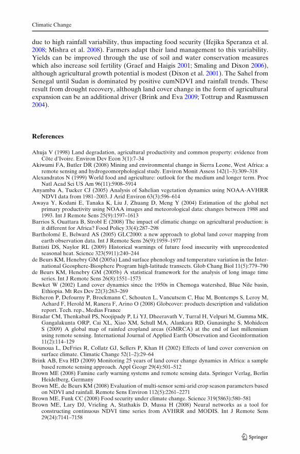
5 Conclusion

We determined average SOS, LOS, maxNDVI and cumNDVI, and their variabilityand trends for nine farming systems of sub-Saharan Africa using AVHRR NDVItime series between 1982 and 2005. Phenological characterization of the systems waspossible, although substantial spatial variation is present within systems. Seasonallycumulated NDVI (cumNDVI) was the principal phenological metric in this paperas it relates to net primary productivity. Temporal variation of cumNDVI is highestin semiarid and subhumid farming systems, which implies important year to yearvariation of available natural resources. Climate is an important driver for thisvariation, as well as for trends. Positive cumNDVI trends are found in a large regionstretching from Senegal to South Sudan covering different farming systems. Droughtrecovery since the 1980’s seems to be the strongest factor, which is supported by awetting trend obtained from the CRU data. Regions of negative cumNDVI trendsare concentrated on the south-coast of West Africa and in Tanzania. Drivers includeincreased population pressure, decline of fertilizer use, land degradation, and miningactivities.

We discussed causes of change and variability based on available literature.Although food security comprises more than the local natural resource base, ourresults can provide an input for food security analysis by identifying zones of highvariability or downward trends. However, results presented here should be seenas a starting point for more detailed fine-scale analysis. In view of current climatescenarios predicting a large impact on African agriculture, continued monitoring andtime series analysis of phenology metrics seems indispensable. Coarse-scale analy-sis based on high-frequency temporal information permits identifying large-scalechanges and areas/farming systems of particular concern for food insecurity. Thediversity and trends within farming system boundaries suggest that farming systemsare dynamic.

Acknowledgements The AVHRR data were provided by J.E. Pinzón and M.E. Brown (2007),Global Inventory Modeling and Mapping Studies, Global Land Cover Facility, University ofMaryland, College Park, Maryland. The authors would like to thank Mauro Michielon for hisassistance in processing the GFS and GAUL vector data. We thank Oscar Rojas and four anonymousreviewers for their helpful comments on the manuscript.

Open Access This article is distributed under the terms of the Creative Commons AttributionNoncommercial License which permits any noncommercial use, distribution, and reproduction inany medium, provided the original author(s) and source are credited.

Appendix A: Discussion of results per farming system

This appendix provides a short overview of the farming systems studied. Per system,main characteristics are described and the results of the phenological analysis of

Climatic Change

this study are summarized. We explore potential drivers of change for the selectedfarming systems based on our climate analysis and published literature. This ex-ploration is not exhaustive, but intended as a potential starting point for otherresearchers to conduct studies in their local areas of expertise and regions of study toexpand upon our results.

A.1 Tree crop (TC)

The TC farming system combines industrial tree crops with inter-planted food crops,grown for subsistence. Crop failure is not common within TC (Dixon et al. 2001).The negative cumNDVI trend that we find in TC of West Africa could be a resultof the increased population pressure on natural resources (Brink and Eva 2009), theneglect of some industrial tree crops following decreasing profitability (Dixon et al.2001), and deteriorating community controls on common lands (Ahuja 1998). Whilemany TC regions are rather stable, within Ivory Coast greater variability is apparent.Although the negative trend here is significant, the higher CVt may partially becaused by remaining cloud effects in the GIMMS dataset. In Ivory Coast and Liberianegative cumNDVI trends co-occur with negative trends in LOS and maxNDVI.CRU data show a wetting trend for Liberia, but more commonly a warming trend(Sierra Leone, Ivory Coast, Cameroon southwards). Land cover conversions in thisfarming system could well be a partial cause of this trend (Bounoua et al. 2002).

A.2 Rice-tree crop (RT)

The RT system is solely found in humid areas of Madagascar. Agricultural potentialis high, but small farm sizes, lack of suitable technologies, and poor markets causepoverty to prevail (Dixon et al. 2001; Minten and Barrett 2008). CumNDVI resultsshow a spatially homogeneous system with little temporal variability. In Antana-narivo and Toamasina provinces (center and east Madagascar) negative trends arefound, likely caused by deforestation and agricultural expansion (Harper et al. 2007;McConnell et al. 2004). In addition, the CRU data show a significant warming trendfor the entire system which may indicate a decline of water availability throughhigher evaporation losses. No precipitation trends are found.

A.3 Highland perennial (HP)

This system is situated in subhumid and humid highland zones of the East AfricanHighlands. Of all SSA farming systems, it has the highest population density withconsequently very small land holdings and high levels of poverty (Dixon et al.2001). CumNDVI is relatively high and stable, although East-Congo, Rwanda, andBurundi show somewhat lower levels. Significant negative cumNDVI trends areonly found in Rwanda, which match with a negative maxNDVI trend (Fig. 7a). Apossible explanation is the reported widespread ongoing land degradation (Lewisand Nyamulinda 1996; Rutunga et al. 2007), which constituted the basis for the warin the 90’s (Gasana 2002). The HP system has experienced significant warming since1982 based on CRU data. However, a clear impact of this warming on phenologycannot be discerned.

Climatic Change

A.4 Highland temperate mixed (HT)

The HT farming system has the second highest population density and is chieflyfound in the Ethiopian highlands. Problems include soil erosion, fertility decline,and lack of inputs. Weather-related crop failures are common (Dixon et al. 2001).Our results show varying levels of cumNDVI depending on location, but generallylittle temporal variation and trends. This agrees with the reported absence of rainfalltrends over HT in Ethiopia (Cheung et al. 2008). However, the CRU analysis showsfor most of Ethiopia under HT a wetting and warming trend. The problems, cropfailures and climate trends described here do not imply a great reduction of overallvegetation activity as observed from our AVHRR analysis. It is however possiblethat finer-scale vegetation trends occur in the very heterogeneous environmentof Ethiopia. These may also be positive trends, for example due to reforestation(Bewket 2002).

A.5 Root crop (RC)

The RC system is found in humid areas. It has a limited risk to crop failure and lowpoverty levels (Dixon et al. 2001). LOS, maxNDVI, and cumNDVI are among thehighest of all farming systems with slightly lower levels of maxNDVI and cumNDVIin the West African portion. CumNDVI variability is relatively low. A big fractionof the system experiences positive cumNDVI trends (Ghana to South Sudan, plusAngola and southern Congo). These correspond to positive LOS trends (Fig. 7a),which are also found by Heumann et al. (2007). Part of this area also shows positiverainfall trends. Negative cumNDVI trends in Sierra Leone may be explained bymining activities and consequent land use changes (Akiwumi and Butler 2008), whilethose in Tanzania are discussed in Section A.7.

A.6 Cereal-root crop mixed (CR)

This farming system is situated in dry subhumid regions. It is marked as havingexcellent prospects for agricultural growth due to abundant agricultural land and lowpopulation densities, which makes the natural resource base underutilized (Dixonet al. 2001). CumNDVI above the equator has significantly lower values than below,due to a shorter LOS. Variability of cumNDVI is low to average, while the northernpart is fully included in the large region of positive cumNDVI trends. These aresupported both by positive maxNDVI and LOS trends and correspond to therecovery of drought in the 1980’s (Dai et al. 2004; Heumann et al. 2007), whichalso shows in our CRU rainfall analysis. South of the equator only Bié and Uígeprovinces of Angola and a part of north-western Zambia show positive cumNDVItrends, supported by a positive LOS trend.

A.7 Maize mixed (MM)

The MM system is located in dry to moist subhumid regions. Although agriculturalprospects are judged to be good, the system is in crisis due to a sharp fall of input useand high fertilizer prices (Dixon et al. 2001). Varying mean cumNDVI levels indicatethat high spatial variability is present within this system. Temporal variability (CVt)

Climatic Change

for MM has a strong negative relation with mean cumNDVI levels (r = −0.69), whichimplies higher vulnerability to food insecurity in low cumNDVI areas, such as Kenya.National maize production figures for Kenya support this high variability (Rojas2007). Western Ethiopia MM areas fall in the large band of positive cumNDVItrends. A large region of negative trends occurs in central Tanzania, which issupported by negative trends of LOS and maxNDVI. These negative trends alsooccur in the RC system (Section A.5). One causing factor is likely to be the strongdecline in fertilizer use since 1990 due to market liberalization and consequent priceincreases (Malley et al. 2009; Skarstein 2005). Based on our own analysis of nationalFAOSTAT fertilizer consumption data, most other MM countries show positivetrends in this time period, although more recent declines occur (e.g. Zimbabwe).Nonetheless, positive trends in fertilizer consumption may be compensated for byincreasing crop areas, hence still lowering the fertilizer use per hectare. A secondfactor for declining cumNDVI is a reported rainfall decrease and the increase ofdry spells (Enfors and Gordon 2007; Giannini et al. 2008; Schreck III and Semazzi2004; Slegers 2008). Our CRU analysis does not show a decrease in rainfall for 1982–2006, although a significant warming trend is observed, which may imply higherevaporation losses and hence drier conditions. Other potential drivers are rapidpopulation growth and soil fertility decline (Enfors and Gordon 2007; Malley et al.2009) causing an increased pressure on available natural resources. These processesresult in declining maize surpluses thus threatening national food security (Dixonet al. 2001).

A.8 Large commercial & smallholder (LC)

The LC farming system comprises scattered smallholder and large-scale commercialfarming in semiarid and dry subhumid zones of South Africa and Namibia. Povertyamong smallholders is severe due to poor soils and frequent droughts (Dilley 2000;Dixon et al. 2001). Mean cumNDVI is generally low, while temporal variabilityvaries from low in Eastern Cape and western provinces of South Africa (SA) tohigh in the drier Northern Cape province (SA) and Namibia. CumNDVI is stronglylinked to annual rainfall (Helldén and Tottrup 2008; Wessels et al. 2007). Significantpositive trends of cumNDVI are found in Northern Cape, North West, and FreeState provinces (SA), which for the first two mentioned provinces are supported bypositive CRU rainfall trends. In semiarid systems, SOS variability is an importantcharacteristic affecting crop production (Brown and de Beurs 2008; Tadross et al.2005). SOS temporal variability of Fig. 4 corresponds well with the SOS variabilitymap by Tadross et al. (2005) derived from a product based on rain gauge data only,with lower values occuring in eastern SA.

A.9 Agro-pastoral millet/sorghum (AP)

Crop production and livestock are of similar importance in the AP farming system.It is situated in semiarid zones and pressure on available natural resources is high.Crop failures are mostly attributed to droughts and poverty is extensive (Dixon et al.2001). Together with the LC system, mean cumNDVI values are among the lowest(Table 1) and closely linked to rainfall and soil moisture availability (Nicholson et al.1990). Furthermore, the cumNDVI temporal variation is generally very high (Fig. 5)

Climatic Change

due to high rainfall variability, thus impacting food security (Ifejika Speranza et al.2008; Mishra et al. 2008). Farmers adapt their land management to this variability.Yields can be improved through the use of soil and water conservation measureswhich also increase soil fertility (Graef and Haigis 2001; Smaling and Dixon 2006),although agricultural growth potential is modest (Dixon et al. 2001). The Sahel fromSenegal until Sudan is dominated by positive cumNDVI and rainfall trends. Theseresult from drought recovery, although land cover change in the form of agriculturalexpansion can be an additional driver (Brink and Eva 2009; Tottrup and Rasmussen2004).

References

Ahuja V (1998) Land degradation, agricultural productivity and common property: evidence fromCôte d’Ivoire. Environ Dev Econ 3(1):7–34

Akiwumi FA, Butler DR (2008) Mining and environmental change in Sierra Leone, West Africa: aremote sensing and hydrogeomorphological study. Environ Monit Assess 142(1–3):309–318

Alexandratos N (1999) World food and agriculture: outlook for the medium and longer term. ProcNatl Acad Sci US Am 96(11):5908–5914

Anyamba A, Tucker CJ (2005) Analysis of Sahelian vegetation dynamics using NOAA-AVHRRNDVI data from 1981–2003. J Arid Environ 63(3):596–614

Awaya Y, Kodani E, Tanaka K, Liu J, Zhuang D, Meng Y (2004) Estimation of the global netprimary productivity using NOAA images and meteorological data: changes between 1988 and1993. Int J Remote Sens 25(9):1597–1613

Barrios S, Ouattara B, Strobl E (2008) The impact of climatic change on agricultural production: isit different for Africa? Food Policy 33(4):287–298

Bartholomé E, Belward AS (2005) GLC2000: a new approach to global land cover mapping fromearth observation data. Int J Remote Sens 26(9):1959–1977

Battisti DS, Naylor RL (2009) Historical warnings of future food insecurity with unprecedentedseasonal heat. Science 323(5911):240–244

de Beurs KM, Henebry GM (2005a) Land surface phenology and temperature variation in the Inter-national Geosphere-Biosphere Program high-latitude transects. Glob Chang Biol 11(5):779–790

de Beurs KM, Henebry GM (2005b) A statistical framework for the analysis of long image timeseries. Int J Remote Sens 26(8):1551–1573

Bewket W (2002) Land cover dynamics since the 1950s in Chemoga watershed, Blue Nile basin,Ethiopia. Mt Res Dev 22(3):263–269

Bicheron P, Defourny P, Brockmann C, Schouten L, Vancutsem C, Huc M, Bontemps S, Leroy M,Achard F, Herold M, Ranera F, Arino O (2008) Globcover: products description and validationreport. Tech. rep., Medias France

Biradar CM, Thenkabail PS, Noojipady P, Li YJ, Dheeravath V, Turral H, Velpuri M, Gumma MK,Gangalakunta ORP, Cai XL, Xiao XM, Schull MA, Alankara RD, Gunasinghe S, MohideenS (2009) A global map of rainfed cropland areas (GMRCA) at the end of last millenniumusing remote sensing. International Journal of Applied Earth Observation and Geoinformation11(2):114–129

Bounoua L, DeFries R, Collatz GJ, Sellers P, Khan H (2002) Effects of land cover conversion onsurface climate. Climatic Change 52(1–2):29–64

Brink AB, Eva HD (2009) Monitoring 25 years of land cover change dynamics in Africa: a samplebased remote sensing approach. Appl Geogr 29(4):501–512

Brown ME (2008) Famine early warning systems and remote sensing data. Springer Verlag, BerlinHeidelberg, Germany

Brown ME, de Beurs KM (2008) Evaluation of multi-sensor semi-arid crop season parameters basedon NDVI and rainfall. Remote Sens Environ 112(5):2261–2271

Brown ME, Funk CC (2008) Food security under climate change. Science 319(5863):580–581Brown ME, Lary DJ, Vrieling A, Stathakis D, Mussa H (2008) Neural networks as a tool for

constructing continuous NDVI time series from AVHRR and MODIS. Int J Remote Sens29(24):7141–7158

Climatic Change

Brown ME, de Beurs KM, Vrieling A (2010) The response of African land surface phenology tolarge scale climate oscillations. Remote Sens Environ 114(10):2286–2296

Camberlin P, Moron V, Okoola R, Philippon N, Gitau W (2009) Components of rainy seasons’variability in Equatorial East Africa: onset, cessation, rainfall frequency and intensity. TheorAppl Climatol 98(3–4):237–249

Cao M, Prince SD, Small J, Goetz SJ (2004) Remotely sensed interannual variations and trends interrestrial net primary productivity 1981–2000. Ecosystems 7(3):233–242

Chen J, Jönsson P, Tamura M, Gu Z, Matsushita B, Eklundh L (2004) A simple method for recon-structing a high-quality NDVI time-series data set based on the Savitzky-Golay filter. RemoteSens Environ 91(3–4):332–344

Cheung WH, Senay GB, Singh A (2008) Trends and spatial distribution of annual and seasonalrainfall in Ethiopia. Int J Climatol 28(13):1723–1734

Cooper PJM, Dimes J, Rao KPC, Shapiro B, Shiferaw B, Twomlow S (2008) Coping better withcurrent climatic variability in the rain-fed farming systems of sub-Saharan Africa: an essentialfirst step in adapting to future climate change? Agric Ecosyst Environ 126(1–2):24–35

Dai A, Lamb PJ, Trenberth KE, Hulme M, Jones PD, Xie P (2004) The recent Sahel drought is real.Int J Climatol 24(11):1323–1331

Dilley M (2000) Reducing vulnerability to climate variability in southern Africa: the growing role ofclimate information. Climatic Change 45(1):63–73

Dixon J, Gulliver A, Gibbon D (2001) Farming systems and poverty: improving farmers’ livelihoodsin a changing world. FAO, Rome and World Bank, Washington DC

Enfors EI, Gordon LJ (2007) Analysing resilience in dryland agro-ecosystems: a case study of theMakanya catchment in Tanzania over the past 50 years. Land Degrad Dev 18(6):680–696

Fermont AM, van Asten PJA, Giller KE (2008) Increasing land pressure in East Africa: the changingrole of cassava and consequences for sustainability of farming systems. Agric Ecosyst Environ128(4):239–250

Friedl MA, McIver DK, Hodges JCF, Zhang XY, Muchoney D, Strahler AH, Woodcock CE, GopalS, Schneider A, Cooper A, Baccini A, Gao F, Schaaf C (2002) Global land cover mapping fromMODIS: algorithms and early results. Remote Sens Environ 83(1–2):287–302

Fritz S, See L (2008) Identifying and quantifying uncertainty and spatial disagreement in the com-parison of Global Land Cover for different applications. Glob Chang Biol 14(5):1057–1075

Fuller DO (1998) Trends in NDVI time series and their relation to rangeland and crop production inSenegal, 1987-1993. Int J Remote Sens 19(10):2013–2018

Funk C, Budde ME (2009) Phenologically-tuned MODIS NDVI-based production anomaly esti-mates for Zimbabwe. Remote Sens Environ 113(1):115–125

Gasana J (2002) Remember Rwanda? World Watch 15(5):24–33Giannini A, Saravanan R, Chang P (2003) Oceanic forcing of Sahel rainfall on interannual to

interdecadal time scales. Science 302(5647):1027–1030Giannini A, Biasutti M, Held IM, Sobel AH (2008) A global perspective on African climate. Climatic

Change 90(4):359–383Glantz MH, Gommes R, Ramasamy S (2009) Coping with a changing climate: considerations for

adaptation and mitigation in agriculture. FAO, Rome, ItalyGoetz SJ, Prince SD, Small J, Gleason ACR (2000) Interannual variability of global terrestrial

primary production: results of a model driven with satellite observations. J Geophys Res105(D15):20,077–20,091

Graef F, Haigis J (2001) Spatial and temporal rainfall variability in the Sahel and its effects onfarmers’ management strategies. J Arid Environ 48(2):221–231

Gregory PJ, Ingram JSI, Brklacich M (2005) Climate change and food security. Philos Trans R Soc,B Biol Sci 360(1463):2139–2148

Harper GJ, Steininger MK, Tucker CJ, Juhn D, Hawkins F (2007) Fifty years of deforestation andforest fragmentation in Madagascar. Environ Conserv 34(4):325–333

Helldén U, Tottrup C (2008) Regional desertification: a global synthesis. Glob Planet Change64(3–4):169–176

Herrmann SM, Anyamba A, Tucker CJ (2005) Recent trends in vegetation dynamics in the AfricanSahel and their relationship to climate. Glob Environ Change 15(4):394–404

Heumann BW, Seaquist JW, Eklundh L, Jönsson P (2007) AVHRR derived phenological change inthe sahel and soudan, africa, 1982-2005. Remote Sens Environ 108(4):385–392

Hickler T, Eklundh L, Seaquist JW, Smith B, Ardö J, Olsson L, Sykes MT, Sjöström M (2005)Precipitation controls Sahel greening trend. Geophys Res Lett 32(21):1–4

Climatic Change

Huete A, Didan K, Miura T, Rodriguez EP, Gao X, Ferreira LG (2002) Overview of the radio-metric and biophysical performance of the MODIS vegetation indices. Remote Sens Environ83(1–2):195–213

Ifejika Speranza C, Kiteme B, Wiesmann U (2008) Droughts and famines: the underlying factorsand the causal links among agro-pastoral households in semi-arid Makueni district, Kenya. GlobEnviron Change 18(1):220–233

Imhoff ML, Bounoua L, Ricketts T, Loucks C, Harriss R, Lawrence WT (2004) Global patterns inhuman consumption of net primary production. Nature 429(6994):870–873

IPCC (2007) Climate change 2007: impacts, adaptation and vulnerability. Contribution of WorkingGroup II to the Fourth Assessment Report of the Intergovernmental Panel on Climate Change.Cambridge University Press, Cambridge, UK

Justice CO, Townshend JRG, Holben BN, Tucker CJ (1985) Analysis of the phenology of globalvegetation using meteorological satellite data. Int J Remote Sens 6(8):1271–1318

Kabanda TA, Jury MR (1999) Inter-annual variability of short rains over northern Tanzania. ClimRes 13(3):231–241

Kurukulasuriya P, Mendelsohn R, Hassan R, Benhin J, Deressa T, Diop M, Eid HM, Fosu KY,Gbetibouo G, Jain S, Mahamadou A, Mano R, Kabubo-Mariara J, El-Marsafawy S, Molua E,Ouda S, Ouedraogo M, Séne I, Maddison D, Seo SN, Dinar A (2006) Will African agriculturesurvive climate change? World Bank Econ Rev 20(3):367–388

Lal R (2007) Anthropogenic influences on world soils and implications to global food security. AdvAgron 93:69–93

Laux P, Kunstmann H, Bardossy A (2008) Predicting the regional onset of the rainy season in WestAfrica. Int J Climatol 28(3):329–342

Lewis LA, Nyamulinda V (1996) The critical role of human activities in land degradation in Rwanda.Land Degrad Dev 7(1):47–55

Liu J, Fritz S, van Wesenbeeck CFA, Fuchs M, You L, Obersteiner M, Yang H (2008) A spatiallyexplicit assessment of current and future hotspots of hunger in Sub-Saharan Africa in the contextof global change. Glob Planet Change 64(3–4):222–235

Lo Seen Chong D, Mougin E, Gastellu-Etchegorry JP (1993) Relating the global vegetation indexto net primary productivity and actual evapotranspiration over Africa. Int J Remote Sens14(8):1517–1546

Lobell DB, Burke MB, Tebaldi C, Mastrandrea MD, Falcon WP, Naylor RL (2008) Prioritizingclimate change adaptation needs for food security in 2030. Science 319(5863):607–610

Malley ZJU, Taeb M, Matsumoto T (2009) Agricultural productivity and environmental insecurityin the Usangu plain, Tanzania: policy implications for sustainability of agriculture. Environment,Development and Sustainability 11(1):175–195

Maxwell DG (1996) Measuring food insecurity: The frequency and severity of “coping strategies”.Food Policy 21(3):291–303

McConnell WJ, Sweeney SP, Mulley B (2004) Physical and social access to land: spatio-temporalpatterns of agricultural expansion in Madagascar. Agric Ecosyst Environ 101(2–3):171–184

Milesi C, Hashimoto H, Running SW, Nemani RR (2005) Climate variability, vegetation productivityand people at risk. Glob Planet Change 47(2–4 SPEC. ISS.):221–231

Minten B, Barrett CB (2008) Agricultural technology, productivity, and poverty in Madagascar.World Dev 36(5):797–822

Mishra A, Hansen JW, Dingkuhn M, Baron C, Traoré SB, Ndiaye O, Ward MN (2008) Sorghum yieldprediction from seasonal rainfall forecasts in Burkina Faso. Agric For Meteorol 148(11):1798–1814

Misselhorn AA (2005) What drives food insecurity in southern Africa? A meta-analysis of householdeconomy studies. Glob Environ Change 15(1):33–43

Mitchell TD, Jones PD (2005) An improved method of constructing a database of monthly climateobservations and associated high-resolution grids. Int J Climatol 25(6):693–712

Nemani RR, Keeling CD, Hashimoto H, Jolly WM, Piper SC, Tucker CJ, Myneni RB, Running SW(2003) Climate-driven increases in global terrestrial net primary production from 1982 to 1999.Science 300(5625):1560–1563

Nicholson SE (1993) An overview of African rainfall fluctuations of the last decade. J Climate6(7):1463–1466

Nicholson SE, Davenport ML, Malo AR (1990) A comparison of the vegetation response to rain-fall in the Sahel and East Africa, using normalized difference vegetation index from NOAAAVHRR. Climatic Change 17(2–3):209–241

Climatic Change

Olsson L, Eklundh L, Ardo J (2005) A recent greening of the Sahel—trends, patterns and potentialcauses. J Arid Environ 63(3):556–566

Parry M, Rosenzweig C, Livermore M (2005) Climate change, global food supply and risk of hunger.Philos Trans R Soc B: Biol Sci 360(1463):2125–2138

Philippon N, Jarlan L, Martiny N, Camberlin P, Mougin E (2007) Characterization of the interannualand intraseasonal variability of West African vegetation between 1982 and 2002 by means ofNOAA AVHRR NDVI data. J Climate 20(7):1202–1218

Pinzón JE, Brown ME, Tucker CJ (2005) Satellite time series correction of orbital drift artifactsusing empirical mode decomposition. In: Huang N, Shen SSP (eds) Hilbert-Huang transform:introduction and applications, World Scientific, Hackensack NJ, pp 167–186

Ramankutty N, Evan AT, Monfreda C, Foley JA (2008) Farming the planet: 1. Geographic distribu-tion of global agricultural lands in the year 2000. Glob Biogeochem Cycles 22(1):GB1003

Reason CJC, Landman W, Tennant W (2006) Seasonal to decadal prediction of southern Africanclimate and its links with variability of the Atlantic Ocean. Bull Am Meteorol Soc 87(7):941–955

Reed BC, Brown JF, Vanderzee D, Loveland TR, Merchant JW, Ohlen DO (1994) Measuringphenological variability from satellite imagery. J Veg Sci 5(5):703–714

Reed BC, Schwartz MD, Xiao X (2009) Remote sensing phenology: status and the way forward.In: Noormets A (ed) Phenology of ecosystem processes: applications in global change research,Springer-Verlag, New York, pp 231–246

Ringler C, Bryan E, Biswas A, Cline SA (2010) Water and food security under global change. In:Ringler C, Biswas AK, Cline SA (eds) Global change: impacts on water and food security,Springer-Verlag, Berlin Heidelberg, pp 3–15

Roerink GJ, Menenti M, Verhoef W (2000) Reconstructing cloudfree NDVI composites usingFourier analysis of time series. Int J Remote Sens 21(9):1911–1917

Rojas O (2007) Operational maize yield model development and validation based on remote sensingand agro-meteorological data in Kenya. Int J Remote Sens 28(17):3775–3793

Rojas O (2009) Crop monitoring in Kenya - August 2009 - MARS Bulletin. Tech. rep., Joint ResearchCentre of the European Commission

Rojas O, Rembold F, Royer A, Negre T (2005) Real-time agrometeorological crop yield monitoringin Eastern Africa. Agronomie 25(1):63–77

Running SW, Nemani RR, Heinsch FA, Zhao M, Reeves M, Hashimoto H (2004) A continuoussatellite-derived measure of global terrestrial primary production. BioScience 54(6):547–560

Rutunga V, Janssen BH, Mantel S, Janssens M (2007) Soil use and management strategy for raisingfood and cash output in Rwanda. J Food Agric Environ 5(3–4):434–441

Savitzky A, Golay MJE (1964) Smoothing and differentiation of data by simplified least squaresprocedures. Anal Chem 36(8):1627–1639

Schreck III CJ, Semazzi FHM (2004) Variability of the recent climate of eastern Africa. Int J Climatol24(6):681–701

Skarstein R (2005) Economic liberalization and smallholder productivity in Tanzania. from promisedsuccess to real failure, 1985-1998. Journal of Agrarian Change 5(3):334–362

Slegers MFW (2008) “If only it would rain”: Farmers’ perceptions of rainfall and drought in semi-aridcentral Tanzania. J Arid Environ 72(11):2106–2123

Smaling EMA, Dixon J (2006) Adding a soil fertility dimension to the global farming systemsapproach, with cases from africa. Agric Ecosyst Environ 116(1–2):15–26

Spearman C (1904) The proof and measurement of association between two things. Am J Psychol15:72–101

Tadross MA, Hewitson BC, Usman MT (2005) The interannual variability on the onset of the maizegrowing season over South Africa and Zimbabwe. J Clim 18(16):3356–3372

Tateishi R, Ebata M (2004) Analysis of phenological change patterns using 1982-2000 AdvancedVery High Resolution Radiometer (AVHRR) data. Int J Remote Sens 25(12):2287–2300

Teuling AJ, Stöckli R, Seneviratne SI (2010) Bivariate colour maps for visualizing climate data. IntJ Climatol. doi:10.1002/joc.2153

Thornton PK, Jones PG, Alagarswamy G, Andresen J (2009) Spatial variation of crop yield responseto climate change in East Africa. Glob Environ Change 19(1):54–65

Tottrup C, Rasmussen MS (2004) Mapping long-term changes in savannah crop productivity inSenegal through trend analysis of time series of remote sensing data. Agric Ecosyst Environ103(3):545–560

Tucker CJ (1979) Red and photographic infrared linear combinations for monitoring vegetation.Remote Sens Environ 8(2):127–150

Climatic Change

Tucker CJ, Pinzón JE, Brown ME, Slayback DA, Pak EW, Mahoney R, Vermote EF, El Saleous N(2005) An extended AVHRR 8-km NDVI dataset compatible with MODIS and SPOT vegeta-tion NDVI data. Int J Remote Sens 26(20):4485–4498

Vrieling A, De Beurs KM, Brown ME (2008) Recent trends in agricultural production of Africabased on AVHRR NDVI time series. In: Proceedings of SPIE - The International Society forOptical Engineering, vol 7104: 71040R

Wessels KJ, Prince SD, Malherbe J, Small J, Frost PE, VanZyl D (2007) Can human-induced landdegradation be distinguished from the effects of rainfall variability? A case study in South Africa.J Arid Environ 68(2):271–297

White MA, Thornton PE, Running SW (1997) A continental phenology model for monitoringvegetation responses to interannual climatic variability. Glob Biogeochem Cycles 11(2):217–234

White MA, de Beurs KM, Didan K, Inouye DW, Richardson AD, Jensen OP, O’Keefe J, Zhang G,Nemani RR, van Leeuwen WJD, Brown JF, de Wit A, Schaepman M, Lin XM, Dettinger M,Bailey AS, Kimball J, Schwartz MD, Baldocchi DD, Lee JT, Lauenroth WK (2009) Intercom-parison, interpretation, and assessment of spring phenology in North America estimated fromremote sensing for 1982-2006. Glob Change Biol 15(10):2335–2359

Zhang X, Friedl MA, Schaaf CB, Strahler AH, Liu Z (2005) Monitoring the response of vegetationphenology to precipitation in Africa by coupling MODIS and TRMM instruments. J GeophysRes 110:D12103