VarEnKF Localisation for an Unstructured Grid

VarEnKF Localisation for an Unstructured Grid

Andreas Rhodin

German Weather Service

Internationsl Symposium on Data Assimilation, Munich 2014

Andreas Rhodin (DWD) VarEnKF for ICON 2014-02-26 1 / 24

1 DWD Global Forecast systemICON Model - Icosahedral Grid with local RefinementsGlobal Data Assimilation Setup

2 VarEnKF BasicsLocalisationTransformed Representation

3 Wavelet TransformationsDiscrete Wavelet transformation (DWT)Transformed Covariance MatricesCharacteristics of Wavelet TransformationsLocalisation in Wavelet Representation


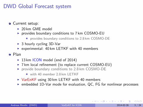
DWD Global Forecast system

Current setup:I 20 km GME modelI provides boundary conditions to 7 km COSMO-EU

F provides boundary conditions to 2.8 km COSMO-DE

I 3 hourly cycling 3D-VarI experimental: 40 km LETKF with 40 members

PlanI 13 km ICON model (end of 2014)I 7 km local refinement (to replace current COSMO-EU)I provide boundary conditions to 2.8 km COSMO-DE

F with 40 member 2.8 km LETKF

I VarEnKF using 30 km LETKF with 40 membersI embedded 1D-Var mode for evaluation, QC, FG for nonlinear processes


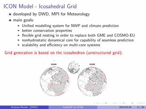
ICON Model - Icosahedral Griddeveloped by DWD, MPI for Meteorology

main goals:I Unified modelling system for NWP and climate predictionI better conservation propertiesI flexible grid nesting in order to replace both GME and COSMO-EUI nonhydrostatic dynamical core for capability of seamless predictionI scalability and efficiency on multi-core systems

Grid generation is based on the icosahedron (unstructured grid):


ICON Model - Icosahedral Grid with local Refinements.

Effective grid spacing(distance betweengrid points):

∆x ≈ 5050n 2k

km

Example:

R3B7: n=3, k=7

1st subdivision by factor of 37 subdivisions by factor of 2

Grid spacing 13: km

Deterministic forecast will run with 13 km resolution

Shall become operational end of 2014


Global Data Assimilation SystemStatus: 3D-Var (operationally) + LETKF (experimental)

GME ens

GME ens

GME ens

GME ens

GME ens

GME ens

GME ens

GME ens

GME detGME det

LETKF

QC obs

obs

3D−Var


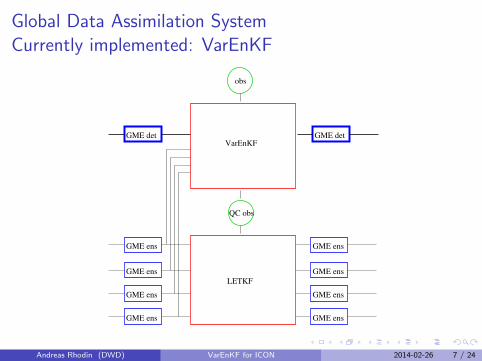
Global Data Assimilation SystemCurrently implemented: VarEnKF

GME ens

GME ens

GME ens

GME ens

GME ens

GME ens

GME ens

GME ens

GME detGME det

LETKF

QC obs

obs

VarEnKF


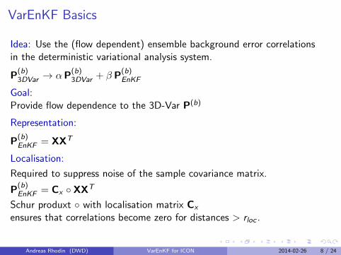
VarEnKF Basics

Idea: Use the (flow dependent) ensemble background error correlationsin the deterministic variational analysis system.

P(b)3DVar → αP

(b)3DVar + β P

(b)EnKF

Goal:Provide flow dependence to the 3D-Var P(b)

Representation:

P(b)EnKF = XXT

Localisation:

Required to suppress noise of the sample covariance matrix.

P(b)EnKF = Cx ◦ XXT

Schur produxt ◦ with localisation matrix Cx

ensures that correlations become zero for distances > rloc .


Multiscale Localisation

Localisation length scales rloc should be different for differentsituations:

I rainy situationsI no rain / high pressure situations

I synoptic scale phenomenaI smaller (convective) scale phenomena

May become important for grid refinement areas


Subsequent 1d-examples for raw and localised sample covariancesare taken from the COSMO-DE (regular) 2.8 km grid

for illustrative purposes


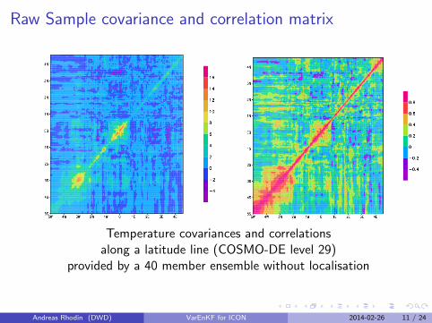
Raw Sample covariance and correlation matrix

Temperature covariances and correlationsalong a latitude line (COSMO-DE level 29)

provided by a 40 member ensemble without localisation


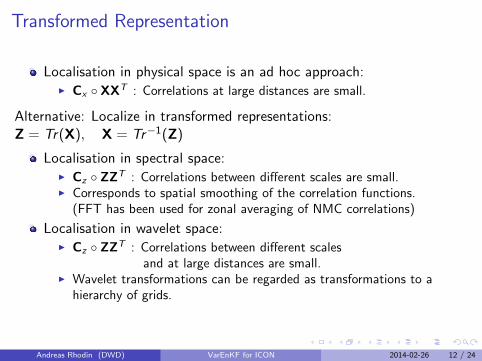
Transformed Representation

Localisation in physical space is an ad hoc approach:I Cx ◦ XXT : Correlations at large distances are small.

Alternative: Localize in transformed representations:Z = Tr(X), X = Tr−1(Z)

Localisation in spectral space:I Cz ◦ ZZT : Correlations between different scales are small.I Corresponds to spatial smoothing of the correlation functions.

(FFT has been used for zonal averaging of NMC correlations)

Localisation in wavelet space:I Cz ◦ ZZT : Correlations between different scales

and at large distances are small.I Wavelet transformations can be regarded as transformations to a

hierarchy of grids.


Discrete Wavelet transformation (DWT)

Fast hierarchical transform with operation count O(n).

coefficients (λ) of the gridded function

λ4,1 λ4,2 λ4,3 λ4,4 λ4,5 λ4,6 λ4,7 λ4,8 λ4,9 λ4,10 λ4,11 λ4,12 λ4,13 λ4,14 λ4,15 λ4,16

low pass high pass↓ ↓

λ3,1 λ3,2 λ3,3 λ3,4 λ3,5 λ3,6 λ3,7 λ3,8 γ3,1 γ3,2 γ3,3 γ3,4 γ3,5 γ3,6 γ3,7 γ3,8


λ2,1 λ2,2 λ2,3 λ2,4 γ2,1 γ2,2 γ2,3 γ2,4 γ3,1 γ3,2 γ3,3 γ3,4 γ3,5 γ3,6 γ3,7 γ3,8


λ1,1 λ1,2 γ1,1 γ1,2 γ2,1 γ2,2 γ2,3 γ2,4 γ3,1 γ3,2 γ3,3 γ3,4 γ3,5 γ3,6 γ3,7 γ3,8

low high↓ ↓

λ0,1 γ0,1 γ1,1 γ1,2 γ2,1 γ2,2 γ2,3 γ2,4 γ3,1 γ3,2 γ3,3 γ3,4 γ3,5 γ3,6 γ3,7 γ3,8

wavelet (γ) and scaling function (λ) coefficients

Coefficients of the transformed vector correspond to the average value(λ) and to the deviations (γ) on different scales.

Inverse transform is a fast hierarchical transform as well.


Wavelet transformed covariance matrices

Wavelet transformations applyindependently to each row andcolumn of a matrix.

Covariances of phenomena at thesame scale are represented by thediagonal blocks.

Covariances of phenomena atdifferent scale are represented byoff-diagonal blocks.

Covariances of phenomena atnearby locations are representedby coefficients in the vicinity ofthe ‘branches’ (diagonals of theblocks).

Only these coefficients areconsiderably different from zero.

0

ψ

ψ

ψψ

ψ ψ ψ ψϕϕ

0 0 1 2 3

0

1

2

3

Block structure of wavelet transformedmatrices


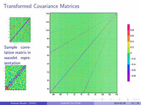
Transformed Covariance Matrices

Sample corre-lation matrix inwavelet repre-sentation

.


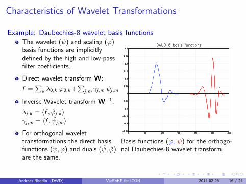
Characteristics of Wavelet Transformations

Example: Daubechies-8 wavelet basis functionsThe wavelet (ψ) and scaling (ϕ)basis functions are implicitlydefined by the high and low-passfilter coefficients.

Direct wavelet transform W:

f =∑

k λ0,k ϕ0,k +∑

j,m γj,m ψj,m

Inverse Wavelet transform W−1:

λj,k = 〈f , ϕ̂j,k〉γj,m = 〈f , ψ̂j,m〉

For orthogonal wavelettransformations the direct basisfunctions (ψ,ϕ) and duals (ψ̂, ϕ̂)are the same.

Basis functions (ϕ, ψ) for the orthogo-nal Daubechies-8 wavelet transform.



The wavelet transform is not unique (as FFT) but many different choicesfor low pass and high pass filter functions exist.

Different desiriable properties cannot be achieved at the same time:

Compact support (for fast transform)

Smoothness (for scale separation)

Orthogonality or bi-orthogonality



Our Choice (so far)

Use Frames:Number of variables in transformed representation is larger.allows smoother basis functions.

Use the Lifting Scheme:allows to define wavelets with desired properties on unstructured grids,splits the wavelet transform into a seqhence of sinmpe operationswhich can easyly be inverted.


Lifting Scheme / Frame

This kind of wavelet transform reduces to a very simple hierarchicalalgorithm:

1 Low pass filter: Average the field (to a coarser grid)

2 High pass filter: Re-interpolate the field to the fine grid and

3 subtract the result from the original one to get the low high passfiltered component.

Iterate the algorithm with the low pass filtered field.

This algorithm can be easyly applied to the ICON gridwhich is generated by a hierachy of grid refinements.


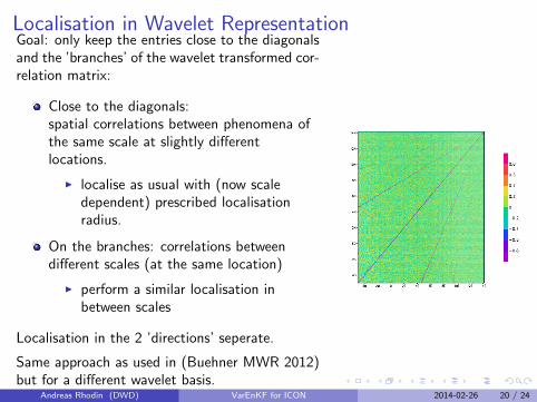
Localisation in Wavelet RepresentationGoal: only keep the entries close to the diagonalsand the ’branches’ of the wavelet transformed cor-relation matrix:

Close to the diagonals:spatial correlations between phenomena ofthe same scale at slightly differentlocations.

I localise as usual with (now scaledependent) prescribed localisationradius.

On the branches: correlations betweendifferent scales (at the same location)

I perform a similar localisation inbetween scales

Localisation in the 2 ’directions’ seperate.

Same approach as used in (Buehner MWR 2012)but for a different wavelet basis.


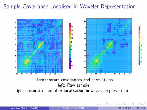
Sample Covariance Localised in Wavelet Representation

Temperature covariances and correlationsleft: Raw sample

right: reconstructed after localisation in wavelet representation


Conclusions

The wavelet lifting scheme provides an efficient method for scaleselective localisation on the unstructured ICON grid.

Thank you for your attention


Spare slides


Sample Covariances

Ensemble x = xmodel − xtrue, true covariance: B = E{x xT

}Unbiased estimate: sample covariance

S =1

N − 1

N∑m=1

(x (m) − x̄

)(x (m) − x̄

)T, E {S} = B

Variance of sample covariance coefficients (Gaussian errors)

σ2ij ≡ E

{(Sij − Bij)

2}

=1

N − 1

[BiiBjj + (Bij)

2]

Error of off-diagonal coefficients dominated by diagonal elements!

EnDA systems rely on Covariances and thus requireI large ensemble sizes (40 . . . 200)I methods to suppress correlations known to be small (localisation)


VarEnKF Localisation for an Unstructured Grid

Documents

Transcript of VarEnKF Localisation for an Unstructured Grid