VaR Approximation MethodsOur study of various approximations to the full revaluation method of computing value at risk using the historical simulation approach reveals alternatives that can significantly reduce processing resources — but at the acceptable expense of accuracy.

Executive Summary“When the numbers are running you instead of you running the numbers, it’s time to take your money off the table.” — Anonymous

Banks and other financial institutions across the world use various approaches to quantify risk in their portfolios. Regulators require that value at risk (VaR), calculated based on the historical data, be used for certain reporting and capital allocation purposes. Currently, this simple risk measure, historical VaR or HsVaR, is computed by some firms using the full revaluation method, which is computationally intensive.

This white paper offers an evaluation of alterna-tive methods to the HsVaR computation that can significantly reduce the processing effort, albeit at the cost of reduced accuracy. The resulting VaR values and the corresponding number of computations for the delta, delta-gamma, and delta-gamma-theta approximation methods were benchmarked against those from the full revalu-ation approach to evaluate the trade-off between the loss of accuracy and the benefit of reduced processing.

Assessing Risk Assessment Value at risk, or VaR as it is widely known, has emerged as a popular method to measure financial market risk. In its most general form,

VaR measures the maximum potential loss in the value of an asset or portfolio over a defined period, for a given confidence level. From a sta-tistical point of view, VaR measures a particular quantile (confidence level) of the return distri-bution of a particular period. Of all the methods available for calculating VaR of a portfolio — parametric, historical simulation and Monte Carlo simulation — the historical simulation approach (HsVaR) alone doesn’t assume any distribution for returns and directly employs actual past data to generate possible future scenarios and determine the required quantile.

Problem StatementCurrently, some financial institutions use the full revaluation method for computing HsVaR. While it is undoubtedly the most straightforward method without any implicit or explicit distributional assumption, a major limitation of using it is that the entire portfolio needs to be valued for every data point of the period under consideration. For example, if 99% — one day — HsVaR is calculated based on the past 500 days of market data of the risk factors, then the HsVaR calculation involves full revaluation of the entire portfolio, 500 times. The method, therefore, requires an intensive computational effort and exerts a heavy load on existing calculation engines and other risk management systems.

• Cognizant 20-20 Insights

cognizant 20-20 insights | september 2012

cognizant 20-20 insights 2

The problem at hand is to explore various approx-imation methods for calculating HsVaR that could reduce the number of computations (valuations) significantly and yet yield an output that is close enough to the full revaluation HsVaR.

Approach and Methodology A hypothetical sample portfolio was considered and various underlying risk factors that determine the value of the portfolio components were identified. Historical data pertaining to those factors was collected. The current price and sensitivities of the portfolio components to the underlying risk factors were then computed. HsVaR was calculated using various methods as detailed below; the results were tabulated to record the deviation of the VaR values computed from approximation methods vis-à-vis the full revaluation method. Further, the numbers of computations involved in each of these method-ologies were compared to observe the benefits accrued from using the approximation methods.

For this study, a portfolio consisting of one long position each on an index ETF (SPDR S&P 500 ETF — a linear instrument), an index call option (on S&P 500 expiring on June 16, 2012 — a nonlinear instrument with short maturity) and a Treasury bond (maturing on Nov. 15, 2019 — a nonlinear instrument with longer maturity) was considered. The objective was to compute a 99% — one day — HsVaR with a settlement date (i.e., date of cal-culation) of Dec. 30, 2011; the historical data used corresponded to the trailing 500 days of market data (Jan. 8, 2010 to Dec. 30, 2011).

The market data related to the underlying risk factors — S&P 500 Index for ETF & call option and yield to maturity (YTM) for the Treasury bond, was collected and the 499 (500 — 1) possible values of the factors for the next day were determined based on past data using this formula:

X(t+1) = X(t) * X(i+1) ... X(i)

Where:

• X(t+1) is the calculated risk factor for the next day.

• X(t) is the value of the risk factor on the day of calculation (Dec. 30, 2011, in this case).

• X(i) and X(i+1) are the value of the risk factors on consecutive days (i = 1 to 500).

Once the possible scenarios of the underlying risk factors for the next day were in place, the corresponding returns (in absolute terms) over the current value were computed. The prices of

the instruments, as on the current date (Dec. 30, 2011), were then computed. The price of the ETF was determined by mapping the underlying returns and the ETF price returns for the past data and the price of index call options was calculated using the Black-Scholes model. The dirty price of the bond was computed using the built-in functions of Microsoft Excel. Finally, the HsVaR of the portfolio was then calculated by using the following methods.

Full Revaluation The HsVaR determined through full revalua-tion (FR) involved calculation of the price of the individual instruments for each of the 499 possible values of the underlying risk factor (a total of 500 valuations including the current day’s price com-putation, for each instrument). From the values of the individual instruments, the portfolio value for each of the scenarios was calculated and then the daily returns were determined (over the current portfolio value). The required quantile (100% — 99% = 1%, in this case) was determined from the sorted list of returns.

Delta ApproximationThe delta approximation (DA) method requires the first order sensitivities (delta, in general, for options; modified duration for bonds) of the individual instruments to be calculated up front. The driving force of this approach is the philosophy that the change in the returns of an instrument can be approximated by multiplying the change in the returns of the underlying with the corresponding sensitivity of the instrument toward the underlying. This approximation works well for linear instruments and tends to deviate for nonlinear instruments:

∆(V) = Delta * ∆(X)

Where:

• ∆(V) is the change in the value of the instrument.

• ∆(X) is the change in value of the underlying.

• Delta is the first order derivative of the instrument with respect to the underlying.

Hence, for all the 499 possible returns of the underlying calculated, corresponding delta returns (absolute dollar returns) of each instrument were computed using the above formula. From the delta returns of the individual instruments, the portfolio returns and the VaR were computed (required quantile of the portfolio returns).

cognizant 20-20 insights 3

Delta-Gamma ApproximationThe delta-gamma approximation (DGA) method is similar to the delta approximation approach, but with a higher order of sensitivity. As portfolios in real life are composed of instruments that are non-linearly related to the underlying risk factors, the delta approximation fares poorly due to the linear assumption involved (as the first order derivative is nothing but the slope of the curve at a given point). The natural remedy to this is to incorporate the next order derivative. The delta-gamma approxi-mation requires the calculation of the second order derivative, gamma, in addition to the delta and the returns of each instrument are calculated as below (derived from the Taylor’s series):

∆(V) = Delta * ∆(X)+ 0.5 * Gamma * ∆(X)2

Where:

• Gamma is the second order derivative of the instrument with respect to the underlying.

From the returns computed using the above formula, the portfolio returns are determined and the required quantile was chosen as the VaR. The delta-gamma method works reasonably well for the simple nonlinear instruments (such as bonds without put/call options) as the curvature of the relationship with the underlying risk factor can be approximated by the convexity measure.

Delta-Gamma-Theta Approximation The delta-gamma-theta approximation (DGTA) approach takes into account an additional term that adjusts for the change in the value of an instrument with respect to time. The partial derivative of the portfolio or instrument with respect to time is added to the above equation to determine the delta-gamma-theta returns and subsequently the VaR is computed:

∆(V) = Delta * ∆(X) + 0.5 * Gamma * ∆(X)2

+ Theta * ∆(T)

Where:

• Theta is the partial derivative of the instrument with respect to time.

• ∆(T) is the change in time (one day in this case).

The DGTA method still accounts only for the second order approximation but incorporates the time effect on the returns (which is ignored in the DGA method).

Note: The model can be further strengthened by adding other sensitivities such as vega (to volatility) and rho (to interest rate). In this study,

we have limited ourselves to theta for the sake of simplicity and ease of understanding.

Assumptions and LimitationsThe objective of the study was to explore various approximations to the full revaluation method and not to statistically validate them. Hence, the methodology employed had the following inherent assumptions to preserve simplicity:

• The study focused on the approximation methods to the full revaluation of the entire portfolio and hence it was assumed that the underlying risk factors for various portfolio components were predetermined and already in place. Accordingly, the study on various methods for choosing the right factors was out of the scope.

• Since the regulatory requirement stipulates that the VaR be calculated based on the historical data, the data points considered in this study are directly taken from the real market historical data without any modifica-tions (i.e., all the data points are actual daily market prices and had equal weight).

• As the objective was to compute one-day VaR, daily market data corresponding to the business days in the period under consider-ation was used (i.e., one-day would mean next business/trading day). The resulting one-day VaR could be easily extended to any “n-day” period by simply multiplying the square root of n to the one-day VaR.

• The problem of full revaluation is more prevalent for over the counter (OTC) products where there is no market data for the trading instruments available. However, for this study, instruments that were very actively traded were chosen so that a simple pricing formula could be employed and the focus would remain on the benefits of approximation methods rather than the complexities of the pricing. Therefore, the computations in the study do suffer from model risk and the inherent assumptions of these pricing functions were applicable here too.

• The six-month Treasury bill rate and implied volatility as calculated from the market prices as on the date of calculation were used, respectively, as the risk-free rate and volatility for calculation of option prices using the Black-Scholes method. Similarly, prices of the ETF were computed directly from the past daily returns by matching the corresponding underlying index returns (as the objective of

cognizant 20-20 insights 4

the ETF was to generate returns correspond-ing to the S&P 500 Index).

• The results of the study were not statistically validated. For real life implementation, the methods used in this paper need to be run on several sets of real market data correspond-

ing to various data windows for thorough validation.

Results and DiscussionFigures 1 and 2 depict the various inputs and outputs of the model:

Figure 1

Figure 3

Figure 2

Input

Portfolio Components ETF Option Bond Total (K)

Number of Instruments 1 1 1 3

Expiry/Maturity Date NA 6/16/2012 11/15/2019

Historical Data 1/8/2010 to 12/30/2011

Settlement Date 12/30/2011

VaR Confidence % 99%

No. of Data Points (N) 500

Output Absolute VaR (in USD)

Method ETF % Diff Option % Diff Bond % Diff Portfolio % Diff

Full Revaluation 4.63 10.26 0.93 14.14

Delta Approximation 4.62 -0.28% 12.19 18.85% 0.94 1.01% 16.07 13.63%

Delta-Gamma Approximation 9.89 -3.63% 0.94 0.54% 13.76 -2.69%

Delta-Gamma-Theta Approximation

10.04 -2.10% 0.93 0.03% 13.91 -1.62%

Note: In the output table above, the “% Diff” values correspond to the deviation of the VaR values calculated through each of the approximation methods from that of the full revaluation method.

As revealed in Figure 2, the delta approximation method yielded results that were close to the full revalu-ation approach (minimum deviation) for the ETF, which is a linear instrument and the delta-gamma-theta approximation for the options and bonds, which is nonlinear. The portfolio VaR corresponding to the DGA and DGTA methods had the DA returns for the ETF combined with second order returns for the option and bond. The benefits of reduced computational stress on the systems can be clearly seen in Figure 3:

MethodNumber of

Valuations^^Number of

ComputationsNumber of

Valuations^^Number of

Computations

FR 1500 3501 K*N (2K+1)N+1

DA 6 3500 2K (2K+1)N

DGA 9 3503 3K (2K+1)N+K

DGTA 12 3506 4K (2K+1)N+2K

K — No. of instruments, N — No. of data points of historical data

^^ Valuations refer to complex calculations that require higher computational power. In this study, we have considered all the calculations involved in pricing instruments and calculating sensitivities as valuations since they require substantial processing power and/or time. The total number of compu-tations, however, includes even straightforward mathematical calculations that are computationally simple and don’t require much system time. Hence, it can be reasonably assumed that the objective of the study is to reduce the number of valuations and not the computations.

cognizant 20-20 insights 5

To understand the benefits of the reduced computations better, Figure 4 quantifies the computational savings for the approximation methods using illustrative scenarios:

Note: As can be seen here, the savings on computational power are huge at ~99% levels and are more evident for longer periods of past data. However, it is worth reiterating that the above savings on com-putational power relate to the number of valuations alone. From the perspective of total number of computations, there isn’t much change, but the stress on the computation engines comes largely from the complex valuations and not simple arithmetic operations.

Scenario -->

Past 500 Days’ Data, 20 Instruments in Portfolio

Past 200 Days’ Data, 20 Instruments in Portfolio

Past 500 Days’ Data, 50 Instruments in Portfolio

MethodNumber of Valuations

Percent Reduction in Number of Valuations

Number of Valuations

Percent Reduction in Number of Valuations

Number of Valuations

Percent Reduction in Number of Valuations

FR 10,000 — 4,000 — 25,000 —

DA 40 99.60% 40 99.00% 100 99.60%

DGA 60 99.40% 60 98.50% 150 99.40%

DGTA 80 99.20% 80 98.00% 200 99.20%

Figure 4

Data requirementsApart from the market data on the underlying factors and the pricing models for all the instru-ments, the following inputs are prerequisites for the above approximation methods.

• Sensitivities of the instruments within a portfolio to all the underlying risk factors (both delta and gamma for each instrument and cor-responding to each risk factor underlying).

Note 1: In the case of the bond portfolio, key rate durations would be required since modified duration would only correspond to a parallel shift in the yield curve. A key rate duration measures sensitivity of the bond price to the yield of specific maturity on the yield curve. In our study, the assumption of parallel shift in the yield curve was made and hence the computations involved only the modified duration of the bond portfolio. However, to improve the accuracy of the results, yield-to-maturity (YTM) values have been modeled from the entire zero coupon yield curve for each of the past data. Similarly, other instru-ments might require specific sets of sensi-tivities (such as option-adjusted duration for bonds with embedded put/call options, etc.)

Note 2: In the case of multivariate deriva-tive instruments whose value depends on more than one underlying risk factor, “cross gammas” for every possible pair of the under-

lying risk factors would be required for each instrument. The current study has assumed only uni-variate instruments (where each instrument has only one underlying risk factor) for the sake of simplicity.

• Theta, or the time sensitivity of all the instru-ments (and other sensitivities such as volatility sensitivity, the vega and the interest rate sen-sitivity, with the rho depending on the model).

The sensitivities can be sourced from the market data providers wherever available (mostly in the case of exchange-traded products).

Comparative AccountEach of the methods discussed in this study has both advantages and shortcomings. To maximize the benefits, banks and financial institutions typically use a combination of these methodolo-gies for regulatory and reporting purposes. Some of the bigger and more sophisticated institutions have developed their internal proprietary approx-imation methods for HsVaR computations that would fall somewhere between the full revalua-tion and the above approximations (variants of partial revaluation methodologies) in terms of accuracy and computational intensity.

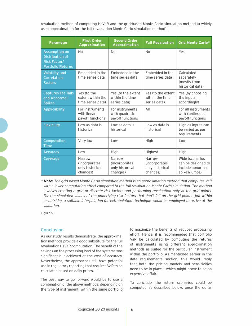
Figure 5 provides a summary of characteristics and differences of the first order (delta) and second order (delta-gamma or delta-gamma-theta) approximation methods vis-à-vis the full

cognizant 20-20 insights 6

revaluation method of computing HsVaR and the grid-based Monte Carlo simulation method (a widely used approximation for the full revaluation Monte Carlo simulation method).

ParameterFirst Order

ApproximationSecond Order

ApproximationFull Revaluation Grid Monte Carlo*

Assumption on Distribution of Risk Factor/Portfolio Returns

No No No Yes

Volatility and Correlation Factors

Embedded in the time series data

Embedded in the time series data

Embedded in the time series data

Calculated separately (mostly from historical data)

Captures Fat Tails and Abnormal Spikes

Yes (to the extent within the time series data)

Yes (to the extent within the time series data)

Yes (to the extent within the time series data)

Yes (by choosing the inputs accordingly)

Applicability For instruments with linear payoff functions

For instruments with quadratic payoff functions

All For all instruments with continuous payoff functions

Flexibility Low as data is historical

Low as data is historical

Low as data is historical

High as inputs can be varied as per requirements

Computation Time

Very low Low High Low

Accuracy Low High Highest High

Coverage Narrow (incorporates only historical changes)

Narrow (incorporates only historical changes)

Narrow (incorporates only historical changes)

Wide (scenarios can be designed to include abnormal spikes/jumps)

Figure 5

* Note: The grid-based Monte Carlo simulation method is an approximation method that computes VaR with a lower computation effort compared to the full revaluation Monte Carlo simulation. The method involves creating a grid of discrete risk factors and performing revaluation only at the grid points. For the simulated values of the underlying risk factors that don’t fall on the grid points (but within or outside), a suitable interpolation (or extrapolation) technique would be employed to arrive at the valuation.

ConclusionAs our study results demonstrate, the approxima-tion methods provide a good substitute for the full revaluation HsVaR computation. The benefit of the savings on the processing load of the systems was significant but achieved at the cost of accuracy. Nevertheless, the approaches still have potential use in regulatory reporting that requires VaR to be calculated based on daily prices.

The best way to go forward would be to use a combination of the above methods, depending on the type of instrument, within the same portfolio

to maximize the benefits of reduced processing effort. Hence, it is recommended that portfolio VaR be calculated by computing the returns of instruments using different approximation methods as suited for the particular instrument within the portfolio. As mentioned earlier in the data requirements section, this would imply that both the pricing models and sensitivities need to be in place — which might prove to be an expensive affair.

To conclude, the return scenarios could be computed as described below; once the dollar

cognizant 20-20 insights 7

return values for the scenarios are in place, HsVaR can be computed at the portfolio level after aggregating the same.

• For linear instruments (such as equity positions, ETFs, forwards, futures, listed securities with adequate market liquidity, etc.), the DA method should be employed.

• For plain vanilla derivative instruments and fixed income products (such as simple bonds, equity options, commodity options, etc.) that are nonlinearly dependent on the underlying factors, the DGTA method would be more suitable.

• For all other highly nonlinear, exotic derivative instruments (such as bonds with call/put options, swaptions, credit derivatives, etc.) and instruments that are highly volatile (or where volatility impacts are not linear) and illiquid, full revaluation methodology is recommended as the approximation methods would yield less accurate values.

Simplification Techniques for Instru-ments that Require Full RevaluationFor the instruments where full revaluation was recommended, the computational burden could be reduced by employing techniques such as data filtering and grid factor valuation. These methods, as explained below, simplify the calcula-tions to a great extent but their accuracy would largely depend on the number and choice of the data points selected for revaluation.

The data filtering technique involves filtering data points relating to the risk factors based on certain criteria (say, top “N” points where the movement of the underlying was either maximum or

minimum or both, depending on the instrument) and performing the revaluation at these chosen points. For other data points, the approximation methods such as DGTA could be employed.

The grid factor valuation, on the other hand, involves choosing a set of discrete data points from the historical risk factors data in such a way that the chosen grid values span the entire data set and form a reasonable representation of the same. The revaluation is done only for these grid values and for all the data points that don’t fall on the grid nodes, a suitable interpolation or extrap-olation technique (linear or quadratic or higher order) is employed to arrive at the value.

Note: Whatever the approximation method chosen, the same data needs to be validated across products for various historical windows before it can be applied to real portfolios. Further, the model needs to be approved by regulators before being used for reporting or capital compu-tation purposes.

In May 2012, the Basel Committee for Banking Supervision (BCBS) released a consultative document to help investment banks fundamentally review their trading books. The report mentioned the committee’s consideration of alternative risk metrics to VaR (such as expected shortfall) due to the inherent weaknesses in VaR of ignoring tail distribution. It should, however, be noted that the approximation methods considered in our study will be valid and useful even for the alternative risk metrics under the committee’s consideration as the approximation methods serve as alterna-tives for returns estimation alone and don’t affect the selection of a particular scenario such as risk metric.

References

• Revisions to the BASEL II Market Risk Framework, BASEL Committee on Banking Supervision, 2009. http://www.bis.org/publ/bcbs158.pdf

• William Fallon, Calculating Value-at-Risk, 1996.

• Linda Allen, Understanding Market, Credit & Operational Risk, Chapter 3: Putting VaR to Work, 2004.

• John C. Hull, Options, Futures, and Other Derivatives, Chapter 20: Value at Risk, 2009.

• Darrell Duffie and Jun Pan, “An Overview of Value at Risk,” 1997.

• Manuel Amman and Christian Reich, “VaR for Nonlinear Financial Instruments — Linear Approximations or Full Monte-Carlo?,” 2001.

• Michael S. Gibson and Matthew Pritsker, “Improving Grid-Based Methods for Estimating Value at Risk of Fixed-Income Portfolios,” 2000.

• Fundamental Review of the Trading Book, BASEL Committee on Banking Supervision, 2012. http://www.bis.org/publ/bcbs219.pdf

About CognizantCognizant (NASDAQ: CTSH) is a leading provider of information technology, consulting, and business process out-sourcing services, dedicated to helping the world’s leading companies build stronger businesses. Headquartered in Teaneck, New Jersey (U.S.), Cognizant combines a passion for client satisfaction, technology innovation, deep industry and business process expertise, and a global, collaborative workforce that embodies the future of work. With over 50 delivery centers worldwide and approximately 145,200 employees as of June 30, 2012, Cognizant is a member of the NASDAQ-100, the S&P 500, the Forbes Global 2000, and the Fortune 500 and is ranked among the top performing and fastest growing companies in the world. Visit us online at www.cognizant.com or follow us on Twitter: Cognizant.

World Headquarters500 Frank W. Burr Blvd.Teaneck, NJ 07666 USAPhone: +1 201 801 0233Fax: +1 201 801 0243Toll Free: +1 888 937 3277Email: inquiry@cognizant.com

European Headquarters1 Kingdom StreetPaddington CentralLondon W2 6BDPhone: +44 (0) 20 7297 7600Fax: +44 (0) 20 7121 0102Email: infouk@cognizant.com

India Operations Headquarters#5/535, Old Mahabalipuram RoadOkkiyam Pettai, ThoraipakkamChennai, 600 096 IndiaPhone: +91 (0) 44 4209 6000Fax: +91 (0) 44 4209 6060Email: inquiryindia@cognizant.com

© Copyright 2012, Cognizant. All rights reserved. No part of this document may be reproduced, stored in a retrieval system, transmitted in any form or by any means, electronic, mechanical, photocopying, recording, or otherwise, without the express written permission from Cognizant. The information contained herein is subject to change without notice. All other trademarks mentioned herein are the property of their respective owners.

About the AuthorsKrishna Kanth is a Consultant within Cognizant’s Banking and Financial Services Consulting Group, working on assignments for leading investment banks in the risk management domain. He has four years of experience in credit risk management and information technology. Krishna has passed the Financial Risk Manager examination conducted by the Global Association of Risk Professionals and has a post-graduate diploma in management from Indian Institute of Management (IIM), Lucknow, with a major in finance. He can be reached at KrishnaKanth.Gadamsetty@cognizant.com.

Sathish Thiruvenkataswamy is a Senior Consulting Manager within Cognizant’s Banking and Financial Services Consulting Group, where he manages consulting engagements in the investment banking, brokerage and risk management domains. Sathish has over 11 years of experience in consulting and solution architecture for banking and financial services clients. He has a post-graduate degree in com-puter-aided management from Indian Institute of Management, Kolkatta. Sathish can be reached at Sathish.Thiruvenkataswamy@cognizant.com.

Credits The authors would like to acknowledge the review assistance provided by Anshuman Choudhary and Rohit Chopra, Consulting Director and Senior Manager of Consulting, respectively, within Cognizant’s Banking and Financial Services Consulting Group.