The WRF Preprocessing System Michael Duda 2006 WRF-ARW Summer Tutorial.
VAPORWRF Data Preparation Guide
VAPORWRF Data and Image
Preparation Guide
January 2012
Web links updated April 2013
Version 21
Introduction This guide is intended to assist scientists to prepare for visualizing WRF-ARW output
using VAPOR VAPOR is the Visualization and Analysis Platform for atmospheric Oceanic
and solar Research WRF is the Weather Research Forecast Model developed at NCAR
(National Center for Atmospheric Research)
This guide also shows (in sections 6 and 7) how VAPOR can also be used to visualize
non-WRF datasets for example these techniques can be used for visualizing 3D data on a grid
that is stretched in the z-dimension or for visualizing data or images on an elevation grid You
can use pressure or other variables to define grid levels (instead of the standard WRF sigma
levels) Section 7 shows how to support geo-referencing and elevation grids with non-WRF
datasets
VAPOR was developed at NCAR with the goal of enabling earth scientists to
interactively perform analysis and visualization of the results of turbulence simulation VAPOR
emphasizes the use of workstation graphics to enable interactive 3D visualization and analysis of
large datasets VAPOR now supports visualization and analysis of WRF-ARW model data
This document covers the following topics
1 Conversion of WRF-ARW output files to a VAPOR data collection (VDC)
WRFVAPOR Data Preparation Guide 2
2 Preparation of geo-referenced images (eg satellite images) to visualize with WRF data
3 Converting NCL plots to be visualized in a WRFVAPOR scene
4 Methods for performing analysis on a WRF VDC for example calculating derived variables
and adding them to the VDC
5 Discussion of how WRF-ARW data is represented and visualized by VAPOR and how best
to use the WRF-specific features of VAPOR
6 Instructions for using the VAPORWRF capabilities to visualize other data sets on similar
grids for example use of these capabilities to visualize data that is on a vertically stretched
grid
7 Use of terrain mapping and geo-referencing with non-WRF data
Note that all of the executables and scripts described in this document require VAPOR to be
installed On Unix platforms these must be run in a shell where vapor-setupsh or vapor-
setupcsh has been sourced
Additional VAPOR Documentation This document provides only basic information useful for preparing data for
visualization and analysis Additional documentation is available to show how to perform
visualization of WRF data using VAPOR All VAPOR documentation is available on the
VAPOR web site at httpwwwvaporucaredu The following documents are particularly
useful for WRF users
The Georgia Weather Case Study a self-guided tutorial that shows how to use
many features of VAPOR to visualize a WRF dataset
VAPOR Userrsquos Guide for WRF Typhoon Research A guide to using VAPOR to
visualize typhoon Jangmi including instructions for preparing satellite images
and NCL plots to visualize in VAPOR
Using Python with VAPOR A guide to defining derived variables using
VAPORrsquos embedded Python interpreter
Using NCL with VAPOR to Visualize WRF-ARW data A step-by-step tutorial
for making images of WRF data in NCL and positioning them in VAPOR scenes
The VAPOR GUI Guide which provides technical explanations of all the
capabilities of the VAPOR user interface
VAPOR Man pages a listing of the capabilities of the various command-line
utilities available with VAPOR
VAPOR is supported by the National Center for Atmospheric Research at Boulder
Colorado USA The VAPOR website at httpwwwvaporucaredu provides downloads
documentation examples etc for VAPOR users VAPOR software is available on the Web at
SourceForge where bug reports and feature requests can also be specified Contact
vaporucaredu with any questions or problems with VAPOR
WRFVAPOR Data Preparation Guide 3
1 Conversion of WRF-ARW data files to a VAPOR VDC
VAPOR can read wrfout files and directly visualize the data however the visualization
performance of VAPOR on very large WRF datasets will be improved if you convert the wrfout files
to a VAPOR Data Collection (VDC) VAPOR provides two command-line utilities (wrfvdfcreate
and wrf2vdf) for this process This process consists of two steps creating a metadata file (a vdf
file) that describes the data set and performing the actual data conversion
The WRF output files to be converted must be in netCDF format and have the following
dimensions west_east south_north bottom_top and their staggered versions and Time The PH
PHB and Times variables must also be present
11 Creating a vdf File (wrfvdfcreate)
A vdf file is an XML file containing metadata describing an entire data set (the output of a
single simulation) for example domain size total number of time steps and variable names A vdf
file is created using the wrfvdfcreate command line utility There are essentially two ways of
running wrfvdfcreate
1 In the first form of the command wrfvdfcreate will scan the set of WRF output files
identifying the variables time steps domain extents etc This information is used to
write a vdf file that is appropriate for describing the VDC that will be created This form
of the wrfvdfcreate command requires only two arguments The name(s) of the wrf
output file(s) and the name of the vdf file that will be created The command syntax is
wrfvdfcreate [options] wrf_ncdf_files vaporfilevdf
The default (specifying no options) works well in most cases By default all floating
point 2D and 3D variables that use the spatial dimensions west_east south_north
bottom_top or their staggered versions will be included in the VDC Additional
command-line options can be specified to control the contents of the VDC for example
specifying that a subset or superset of the variables or time steps will be included These
options are described (with examples) in the wrfvdfcreate man pages
2 If the WRF output files are not available users may specify various parameters as options
to the wrfvdfcreate command that describe the expected WRF output data such as the
data extents the grid dimensions the time stamps in the data etc This (second) form of
the command is fairly difficult to use because it requires a lot of information that is not
easily obtained without the WRF output files The second form of the command and all
its arguments are documented in the wrfvdfcreate man pages
wrfvdfcreate will also output the minimum and maximum longitude and latitude of all of the corners
of the domain(s) This is useful for finding a terrain image that covers all the domain(s) of a WRF
WRFVAPOR Data Preparation Guide 4
dataset
12 Converting WRF data (wrf2vdf)
After a vdf file has been created you can convert a WRF data set in part or in whole You can
convert a subset of the variables time steps and refinement levels specified in the vdf file and still
visualize what data youve converted More variables time steps and refinement levels can be
converted later if desired (provided those variables time steps and refinement levels are specified in
the vdf file) The wrf2vdf command line utility converts one or more WRF output files The syntax
is
wrf2vdf [options] vaporFilevdf wrfFiles
The options to the wrf2vdf command are described in the wrf2vdf man pages These options allow
for example controlling specific variables or time steps to convert
By default the wrf2vdf command will convert all 3D and 2D variables that are specified in the VDC
and will also create a new 3D variable named ldquoELEVATIONrdquo that is needed during VAPOR
visualization to interpolate data from the WRF grid to a Cartesian grid used for visualization and
flow integration
Several additional derived variables may be calculated during the data conversion Note This
capability is deprecated because these variables can (with VAPOR 20 and later) easily be calculated
using the VAPOR Python interface The available derived variables include
PHNorm_ The normalized geopotential (PH+PHB)PHB
UVW_ The three-dimensional wind speed
UV_ The horizontal wind speed
omZ_ Approximate vertical vorticity
PFull_ The full pressure (P+PB)
PNorm_ Normalized pressure (P+PB)PB
Theta_ The potential temperature T+300
TK_ Temperature in Kelvin = Theta((P+PB)100000)0286
These derived variables must be specified with the ndashdervars option of the wrfvdfcreate command in
order to be calculated by wrf2vdf
During the conversion variables defined on staggered grids are averaged to the non-staggered
grids
You can convert netCDF files that are not WRF output as long as they have the same dimension
names and lengths as those found in the WRF output for which the vdf file was created The
variables PH PHB and Times must be present in such a file
2 Preparing terrain images for VAPOR visualization
WRFVAPOR Data Preparation Guide 5
Users can make use of VAPORrsquos geo-referencing capability to correctly insert images of the
earth into a WRF scene Several terrain images of the entire world are pre-installed with
VAPOR These include an image of the earthrsquos surface (ldquoBigBlueMarbletiffrdquo) and several
images of political boundaries such as ldquoUSOutlinetifrdquo
To improve rendering time or to make use of other images you may also want to retrieve images
from the Web covering the specific region you are visualizing VAPOR provides a shell script
ldquogetWMSImageshrdquo that will obtain a satellite image of an arbitrary latitudelongitude region of
the earthrsquos surface and convert that image to a geo-referenced TIFF file that can be properly
placed in a VAPOR scene
Other images not necessarily from a satellite image can be converted to geo-referenced TIFF
files for usage in a VAPOR scene using the application ldquotiff2geotiffrdquo that is included in the
VAPOR distribution
This section explains the usage of both of these two applications
21 getWMSImagesh
getWMSImagesh is a command-line tool for obtaining geo-referenced imagery from the
Internet for use as base-map reference in VAPOR visualizations It is implemented as a bash-
shell script and as such only operates in Unix environments (eg Linux Mac OSX Cygwin on
Windows) The script is bundled with the VAPOR distribution and makes use of tiff2geotiff
described in the next section It is thus imperative that the VAPOR environment variables are
correctly set by sourcing vapor-setupcsh or vapor-setupsh in the shell in which you run this
script The Unix utilities wget or curl are also required as is the convert utility from
Imagemagick for some types of maps1 (see httpwwwimagemagickorg)
The script operates in either a default mode or an expert mode The default mode is intended to
assist most users in acquiring typical base-map imagery One chooses from a small set of
predefined map-types which includes NASA Blue Marble and Landsat imagery maps of
political boundaries rivers etc For users who are knowledgeable on Web Mapping Services
(WMS) expert mode can be used to acquire arbitrary imagery from any WMS-compliant server
In either mode one must first determine the latitude and longitude extents that are needed
Usually you will want to choose these large enough to contain the domain or all domains (with a
moving nest) in the WRF dataset There are several ways of determining these extents One way
is to look at the output of wrfvdfcreate This output includes the minmax longitude and latitude
at the corners of the data This will usually be sufficient when the WRF is not near the north or
south pole If the WRF domain is a polar stereo projection that contains the north or south pole
then the rectangle should go from longitude -180 to longitude +180 and latitude range should
include the polar latitude (+90 or -90) Another way to determine the extents is to load the data
1 Needed when a particular WMS server does not support tiff image format This includes all
the map-types available in the default mode except BMNG and Landsat
WRFVAPOR Data Preparation Guide 6
into the vaporgui application and visualize the 2D WRF variables XLAT and XLON in the 2D
visualizer You can click on the image to find the value of these variables and thereby
determine what latitude and longitude values to include in the retrieved data
Default Mode
In default mode the user chooses a base-map from a small set of predetermined map types The
script is invoked on the command-line as
getWMSImagesh optional parameters minLon minLat maxLon maxLat
where minLon minLat maxLon maxLat are the bounding box values for the area-of-interest in
units of decimal degrees Longitudinal values must be in the range [-180hellip180] while latitudinal
values should range from [-90hellip899999]
By default the requested map will be for NASA Blue Marble at an image size of 1024x768
pixels downloaded to a file named BMNGtiff Several optional command-line switches can
override the default behavior
-m map_name
Where map_name is one of (case-sensitive)
BMNG NASA BlueMarble Next Generation the default
landsat Landsat imagery
USstates US state boundaries
UScounties US state and county boundaries
world world political boundaries
rivers major rivers
-r xres yres
Change the mapimage resolution default is 1024x768
-o imageFilename
Change the name of the requested image file default is map_nametiff
-t
Requests a transparent background
Expert Mode
Expert mode is intended for using the script to fetch an image from any OGC-compliant WMS
server As such one must be highly knowledgeable about WMS technology and protocol
Generally this means knowing how to acquire and interpret the so-called GetCapabilities
document from a server from which to determine the URL for a GetMap request the layer
names that are available and the image-formats the server supports Details of this are beyond
the scope of this document consult the WMS specification at the Open Geospatial Consortiums
website (httpwwwopengeospatialorgstandardswms)
WRFVAPOR Data Preparation Guide 7
Expert mode adds the following command-line options to those of the default mode the first
three options are to be used in lieu of the -m map_name option
-s URL
The URL of the WMS service
-l layername
The name of the requested layer
-f format
The format for the requested image as advertised by the server
-o imageFilename
Change the name of the requested image file default is layernametiff
-z
Requests that the resultant image should be compressed
-d
debug mode does not delete temporaryintermediate files
Examples
To request an image of US counties for the US (latitudes 25 to 50 longitudes -125 to -64) issue the
command
getWMSImagesh ndashm USCounties -125 25 -64 50
It is worth noting that the predefined map-types in the default mode are effectively implemented
via expert-mode parameters and thus provide examples of expert mode use For example the
map-type UScounties is a request to a USGS site for two specific layers (states and county
boundaries ordering is important) of an image-format supported by that site A comparable
request on the command-line using expert options would look like
getWMSImagesh -s
httpimsrefcrusgsgov80wmsconnectorcomesriwmsEsrimapUSGS_EDC_National_Atlas
-l ATLAS_STATES_150ATLAS_COUNTIES_2000 -f imagepng -o UScountiestiff -125 25 -64 50
22 tiff2geotiff
tiff2geotiff is an application that is provided as part of the VAPOR distribution on all
supported platforms tiff2geotiff can be used to insert geo-referencing as well as datetime
stamps into an existing TIFF file tiff2geotiff can be used to specify geo-referencing for a single
image or for a sequence of images in one multi-directory TIFF file
Some of the uses of tiff2geotiff include
If you have a terrain image that you would like to map to the terrain in a VAPOR scene (for
example a road map or a political boundary map) you can convert that image to a tiff image
WRFVAPOR Data Preparation Guide 8
and then apply tiff2geotiff to insert geo-referencing that will enable VAPOR to properly map
it onto the earthrsquos surface
Terrain images are available from various web mapping services For example the URL
httpwwwnasanetworkcomwmsrequest=GetMapampversion=13amplayers=|bmng200401amps
tyles=defaultampbbox=-12525-6450ampwidth=1024ampheight=512ampformat=imagetiff will
return a 1024x512 tiff image of the lonlat rectangle from (-12525) to (-6450) tiff2geotiff
can be used to convert this to a geo-referenced terrain image This is useful on platforms
(such as Windows) where the shell command getWMSImagesh may not work
If you have a sequence of plots (such as produced by NCL or other graphic programs you
can convert these plots to one TIFF file and specify a datetime stamp and (optionally) a map
projection for each plot so that VAPOR can properly position the images in space and time
This is performed by the NCL script wrf2geotiffncl that is described in section 3 of this
document
When your source image(s) are not TIFF images you can convert these to a single TIFF image
using the convert command available from ImageMagick Note that VAPOR may not be able to
handle all the possible compressions such as Jpeg compression that are available in tiff files so
it is a good idea to use the option ldquo-c nonerdquo to tiff2geotiff or to use ldquondashcompress Nonerdquo as an
argument to the convert command
tiff2geotiff is a modified version of the geo-tiff application geotifcp and it supports the many
options of that program You can type ldquotiff2geotiff ndashhrdquo to see all the command-line options
There are three modes in which tiff2geotiff is useful for inserting geo-reference information into
TIFF files for VAPOR visualization
1 tiff2geotiff -4 ldquoproj4_stringrdquo ndashn ldquollx lly urx uryrdquo inputTiffFile outputGeoTiffFile
2 tiff2geotiff -4 ldquoproj4_stringrdquo ndashm dateLatLonFile inputTiffFile outputGeoTiffFile
3 tiff2geotiff ndashM dateFile inputTiffFile outputGeoTiffFile
The first mode is used to insert the same geo-referencing into all images of a tiff file The
second mode is used to insert time stamps and geo-referencing into each image of a tiff file
The third mode is used to just insert time stamps into each image of a tiff file
In the above
Each command converts a TIFF file (inputTiffFile) to a geo-referenced TIFF (geoTiff)
file named outputTiffFile
proj4_string is a quoted string that specifies a map projection as described at the Proj4
wiki If the source tiff image is a longlat projection then the string should be
ldquo+proj=latlong +ellps=sphererdquo indicating that the map projection is the latitudelongitude
projection to a spherical earth Other projections can be used here see
httptracosgeoorgprojwiki for Proj4 documentation The WRF projections supported
by VAPOR include Lambert conformal conic polar stereographic longitudelatitude and
Mercator
dateLatLonFile is a text file with one line for each image in the input TIFF file (Note
In TIFF terminology these images are called ldquodirectoriesrdquo) Each line is of the form
DateTime llx lly urx ury pllx plly purx pury
WRFVAPOR Data Preparation Guide 9
Where
DateTime is a WRF-style datetime stamp of the form yyyy-mm-dd_hhmmss
llx lly urx ury are the longitude and latitude of the lower-left and upper-right
corners of the plot area
pllx plly purx pury are the relative positions of the plot area corners in the full
page (values between 00 and 10 where (00) is the lower-left corner of the
page and (11) is the upper-right corner of the page
dateFile is text file with one line for each image in the input tiff file Each line of the file
consists of a WRF-style datetime stamp of the form yyyy-mm-dd_hhmmss
llx lly urx ury are the longitude and latitude of the lower-left and upper-right corners of
all images in the input TIFF file They must be enclosed in quotes
Examples
Suppose the file ldquowestUStiffrdquo is a tiff image of a map of the western US from latitude
25 to latitude 50 and from longitude -125 to longitude -100 To convert this file to a
geo-referenced tiff file ldquogeorefWestUStiffrdquo issue the following command (all on one
line)
tiff2geotiff -4 ldquo+proj=latlongrdquo ndashn ldquo-125 25 -100 50rdquo
westUStiff georefWestUStiff
Suppose you have a sequence of images in one tiff file ldquohurricanetifrdquo that displays a the
precipitation from a hurricane as it moves across the Gulf of Mexico Suppose also that
these images are on a latlon grid Create a text file ldquoDatelatlonExtentstxt with one line
for each time step Each line would be like the following with a date-time stamp
followed by 4 longitudelatitude extents followed by two zeroes and two ones
2009-09-15_100000 -100 20 -90 30 0 0 1 1
3 Converting NCL plots to display as geo-referenced images in VAPOR visualization
This section describes how to use NCL scripts to create plots of WRF data that can be displayed
in VAPOR scenes Cindy Bruyere has provided an NCL library (WRFUserARWncl) and
numerous scripts to facilitate plotting WRF data with NCL These scripts (which we shall call
WRF-NCL scripts) can be modified to produce geo-referenced TIFF files (geotiffs) which can
be read by VAPOR The example scripts are found at
httpwwwmmmucareduwrfOnLineTutorialGraphicsNCLNCL_exampleshtm For more
information about these scripts refer to the NCL WRF documentation
To illustrate these methods there is an on-line tutorial on the VAPOR website entitled ldquoUsing
NCL with VAPOR to Visualize WRF-ARW datardquo That document shows how three different
NCL scripts can be converted to geotiffs and displayed in VAPOR
WRFVAPOR Data Preparation Guide 10
The conversion process involves modifying a WRF-NCL script to generate a geo-referenced
TIFF (geoTiff) file of the plots which can then be incorporated into a VAPOR visualization
session The process generally involves making minor modifications at three key points in the
script after opening the workstation after plot that is to be captured and before exiting the
script There are two additional constraints the workstation type must be postscript and frame-
advance between plots must be explicitly managed
Note that you should only produce one plot for each time step of the data If your NCL script
produces multiple plots for each time step it should be modified to only produce one of the plots
at each time step You can visualize multiple images in the vapor scene at the same time step
however these images need to be in different geoTiff files To visualize multiple plots per time
step you can make multiple geoTiffs by using several NCL scripts one for each of the different
plots
When the NCL plots are horizontal mapped to the WRF domain then the resulting geoTiffs will
be aligned to match the geo-referencing when shown in VAPOR However if the plot is
vertical it will not be geo-referenced and it must be aligned by the VAPOR user to correctly fit
in the coordinates of the domain
Four sample NCL scripts are provided in the VAPOR distribution in the directory
$VAPOR_HOMEsharevapor-xxxexamplesNCL where xxx is the VAPOR version number
(On Windows systems these are located in $VAPOR_HOMEshareexamplesNCL) These
scripts are wrf_cloudncl wrf_EtaLevelsncl wrf_pvncl and wrf_surfacencl and are
modifications of scripts of the same names provided on the NCL-WRF example web page noted
above To use these scripts you will need to edit them to change the names of the wrf output
files that are specified in the scripts
Note that for wrf2geotiffncl to work correctly you must have the file ldquohluresfilerdquo in your Unix
home directory A sample file is at httpwwwnclucareduDocumentGraphicshluresshtml
Overview
A typical WRF-NCL script for plotting WRF data is of the general form
load supporting libraries
load
open WRF fileshellip
hellip
open workstation
wks = gsn_open_wks(ps wrfPlot)
set up resources generate contours etc
hellip
overlay the plot on a map
WRFVAPOR Data Preparation Guide 11
plot = wrf_map_overlay(wrfFile wks (contour) pltres
mapres)
It is also common to see the plot-generation code segment inside a loop over time or over a
collection of files
loop over each timestamp
do i=0 numTimes-1
plot = wrf_map_overlays()
end do
Modifying scripts for geotiff output
The script below shows the previous example modified to generate a geotiff file the new lines
of code are shown in color The keys point to note are i) inclusion of the wrf2geotiff library ii)
opening the geotiff output process iii) setting resources for explicit frame advance iv) writing
each plot to the geotiff output process and v) closing the geotiff output process Note that in
opening the geotiff output process an opaque variable is created that should be passed to other
calls to the wrf2geotiff library The full wrf2geotiff library and the meaning of parameters passed
to the functions follows below
load supporting libraries
load supporting libraries
load
NOTE On Windows the file wrf2geotiffncl is located in
$VAPOR_HOMEshareexamplesNCL
However if the path to $VAPOR_HOME contains blank characters
you should copy the file wrf2geotiffncl to another directory
and load it from that directory in the load statement below
NCL will not correctly handle blanks
in directory names
load the wrf2geotiff library
load $VAPOR_HOMEsharevapor-150examplesNCLwrf2geotiffncl
open WRF fileshellip
open workstation
wks = gsn_open_wks(ps wrfPlot)
this must be performed once after opening a workstation
but before plots are generated It creates an opaque
object that is passed to other wrf2geotiff functions
wrf2gtiff = wrf2geotiff_open(wks)
IMPORTANT
You must explicitly manage frame-advance Here we modify the
WRFVAPOR Data Preparation Guide 12
resource that gets passed to wrf_map_overlays below
pltres = True
pltresFramePlot = False well make frame advance below
loop over each timestamp
do i=0 numTimes-1
plot = wrf_map_overlays()
write the plot just created and advance the frame
wrf2geotiff_write(wrf2gtiff wrfFile times(it) wks
plot True)
frame(wks) frame-advance
end do
close the geotiff file
wrf2geotiff(wrf2gtiff wks)
The wrf2geotiff library
wrf2geotiff_open(wks)
Called once to open a geotiff file for writing The name of the geotiff file will be the
same as the output file of the workstation except with a suffix of gtif
Parameters
wks the workstation object
Returns
An opaque object that is passed to subsequent wrf2geotiff functions
wrf2geotiff_write(wrf2gtif wrfFile timeStamp wks plotObject cropped)
Called for each plot that is to be written to the geotiff file
Parameters
wrf2gtif the opaque object created by the call to wrf2geotiff_open()
wrfFile the WRF input file used to generate the plot used here to extract
georeferencing information
timeStamp a timestamp string typically obtained from the WRF file
wks the workstation object plotObject the plot object to be written
cropped a boolean indicating whether the plot should be cropped at the plot
frame Setting this to false causes the plot and its surrounding
WRFVAPOR Data Preparation Guide 13
labelingannotations to be written into the geotiff
Returns
Nothing
wrf2geotiff_close(wrf2gtiff wks)
Called once after all output has been written to workstation This call has the side-effect
of closing and flushing all pending operations on the workstation such that any
subsequent attempts to use the workstation will be undefined
Parameters
wrf2gtif the opaque object created by the call to wrf2geotiff_open()
wks the workstation object
Returns
Nothing
Advanced functions
wrf2geotiff_setOutputScale(wrf2gtif scaleFactor)
By default images in the geotiff are of the same size in pixels as the postscript page when
rasterized This function can be used to scale the images to something smaller or larger Applies
to the entire collection of plots and if called more than once the scaleFactor of the last plot is
what is used
Parameters
wrf2gtif the opaque object created by the call to wrf2geotiff_open()
scaleFactor a multiplier for the image size
Returns
Nothing
wrf2geotiff_disableGeoTags(wrf2gtif scaleFactor)
Vapor automatically positions geotiff images into a scene But it can also allow a user to
interactively position images that are not georeferenced In particular plots of WRF data that are
vertical cross-sections have nonsensical geo-coordinates (a non-zero area is required) Calling
this function prevents geotiff tags from being written to the tiff file As the timestamps are still
written into the tiff file the user can place the image interactively and Vapor can animate it
through time
Parameters
wrf2gtif the opaque object created by the call to wrf2geotiff_open()
WRFVAPOR Data Preparation Guide 14
Returns
Nothing
Usage Notes
required external programs psplit convert tiff2geotiff
These external programs must be available and visible via the users PATH environment
variable psplit is distributed with NCL and tiff2geotiff is part of the VAPOR
distribution convert is part of the ImageMagick suite of image processing tools which
is commonly part of most Linux distributions and is freely downloadable from the Web
Use of tmp
The conversion to geotiff creates various intermediate files These are written to the tmp
directory and they are generally removed after use Depending upon the size of the
resultant geotiff a fair amount of temporary disk space can be required Experiments
with Hurricane Ike simulation data have resulted in geotiffs of several hundred
megabytes for an image composed of 100+ framestimesteps The amount of required
temporary space is comparable to the size of the resultant geotiff file
Future Plans
Ultimately it is preferable to generate geotiff output directly from NCL Efforts are currently
underway in NCLs development that will facilitate this Such a capability will eliminate
much if not the entire requirement to modify scripts in the manner described herein
4 Performing analysis of WRF data with VAPOR visualization
VAPOR is intended to be used to investigate and understand WRF output data During the
visualization of a WRF data set it is often the case that additional variables need to be calculated
in order to explain the results VAPOR supports three different ways to do this
The easiest method of defining new variables is to use VAPORrsquos Python interface New
variables can be defined as mathematical expressions of existing variables or the full capabilities
of the Python language and associated modules can be utilized VAPOR provides a module of
WRF-specific functions to derive useful variables such as radar reflectivity cloud-top height
vorticity potential vorticity relative humidity sea-level pressure temperature in degrees Kelvin
dewpoint temperature equivalent potential temperature and horizontal wind shear The VAPOR
Python guide Using Python with VAPOR provides full instructions for using this capability
Variables that have been calculated in another program can be added to the VDC
These variables can either be in NetCDF or binary format
WRFVAPOR Data Preparation Guide 15
The VAPOR user can specify a region and time step in the data being visualized
Then using the VAPOR ldquoExportrdquo option in the File menu this information can be
used by an IDLreg
session to calculate additional variables for the specified region and
time The calculated variables can then be imported back into the VAPOR session
and visualized with the other data
This section provides instructions for the latter two operations (not using Python)
41 Adding variables to an existing WRF VAPOR VDC
411 Requirements
Data that is visualized in VAPOR must first be converted into the VAPOR data format This
is the same process as is performed by wrf2vdf (see section 11) The conversion is necessary
because VAPOR represents the data in a multi-resolution (wavelet) format to enable rapid
access to large data The conversion is not time consuming requiring approximately the time to
read and to write the data Variables must meet the following requirements
Variables may be either on two- or three-dimensional grids
Variables may be either single or double precision
Variable data may be either in binary (raw) format or in a NetCDF file Data from other
formats must first be converted to binary or NetCDF files using for example NCL
Variables that are added to a WRF VDC must use the same array dimensions as the WRF
data Two dimensional arrays must have the same size as the west_east and south_north
dimensions (or their staggered versions) in the original WRF output data Three-
dimensional arrays must also agree with the bottom_top or bottom_top_stag dimension of
the WRF data Conversion of data on staggered grids is only supported from NetCDF
files
If the variable data is on a sub-array of the array in the WRF VDC (using a subset of the
horizontal array dimensions of the WRF data) then the data may be converted from
binary files
412 Conversion steps
To add variable data to a VAPOR VDC perform the following two steps
1 Use vdfedit to modify the metadata (vdf file) that describes the data to include the new
variable andor time-steps that will be added This is not necessary if the VDC metadata
already specifies the time step and the variable name The capabilities of vdfedit are
described in the vdfedit man pages
2 Convert the source data to the VAPOR VDC There are three ways to do this
WRFVAPOR Data Preparation Guide 16
If the data is in binary format you can use the command-line utility raw2vdf to convert
the data This utility must be applied once for each time step and each variable
raw2vdf requires that the raw data be on the un-staggered grid
If the data is in NetCDF files it is easiest to convert the data using wrf2vdf This is
possible only if your NetCDF files are consistent with the WRF output files that were
used to create the original VDC (created using wrfvdfcreate) By ldquoconsistentrdquo it is
meant that your NetCDF file uses a ldquoTimesrdquo variable having time stamp values that occur
in the original WRF output and that the NetCDF file has the same standard WRF
dimensions as were used in the WRF output (ie the dimension names west_east
west_east_stag south_north south_north_stag bottom_top and bottom_top_stag must
be in the NetCDF files) When using wrf2vdf to convert new variables you should
specify the ldquo-noelevrdquo option so that wrf2vdf will not attempt to recalculate the
ELEVATION variable from your NetCDF files wrf2vdf can convert any number of
variables and time steps in one invocation By default it will convert all of the variables
that are in both the VDC and in the NetCDF files
Note It is easy in NCL or in IDL to create NetCDF files that are consistent with the
WRF output files use the Times variable and the dimensions from the existing NetCDF
files to specify the Times variable and dimensions in the new file
If the data is in a NetCDF file but the file is not consistent with the WRF output files
you can use the command-line utility ncdf2vdf to convert the data This utility must be
applied once for each time step and for each variable You will need to identify the
names of the three dimensions that will be used If the variable data is dimensioned by
time or any other dimensions (other than the spatial dimensions) then these dimensions
must be specified as ldquoconstant dimensionsrdquo If the data is on a staggered grid (sized one
larger than the VDC dimensions) then ncdf2vdf will interpolate the data to the
unstaggered grid
42 Exporting and Importing data between a WRFVAPOR session and an IDL session
IDL is an interpreted language available from Exelis (httpwwwexelisviscom ) that
efficiently supports array operations and many numerical operators VAPOR supports using IDL
with VAPOR by means of a library of IDL routines that can read and write data from a VAPOR
VDC VAPORrsquos IDL support is documented in the VAPOR IDL Extension Reference Manual
An example of using VAPOR with IDL is provided in Section 5 of the VAPOR Quick Start
Guide VAPOR installation provides a number of IDL examples in the directory
$(VAPOR_SHARE)examplesidl
IDL can be used to calculate new variables and insert them into a VAPOR VDC For
example there is provided an IDL script ldquoAddWRFCurlprordquo in the examplesidl directory This
script can be used to calculate the vector curl of three variables in a WRF VDC and to add the
resulting vector field back into the VDC
WRFVAPOR Data Preparation Guide 17
IDL can also be used to interactively calculate variables that you can immediately
visualize in your current session This is slightly different from the capabilities of IDL analysis
using non-WRF data With WRF data it is required that the variables be calculated in a region
that has the full vertical extents of the WRF data
To interactively perform IDL analysis from a VAPOR session perform the following
steps
1 While visualizing your data from the VAPOR user interface (vaporgui) use the region
manipulator (or specify values in the Region panel) to identify the spatial extents where
you want to calculate the new variable(s) Note that with WRF data this region must be
maximal in the vertical coordinate ie the region must have the same vertical extents as
the full data
2 From the VAPOR Data menu select ldquoExport to IDLrdquo
3 From the IDL session run an IDL script that calculates the variable(s) you need on the
specified region and at the current time step An example of such a script is provided in
the examplesidl directory ldquoWRFVortMagExprordquo This script calculates the
magnitude of vorticity based on the wind velocity in the region
4 From the VAPOR Data menu select ldquoMerge (Import) a Dataset into Current Sessionrdquo
Specify the vdf file that was created by your IDL script You will see that the variable
you have calculated is now available for visualization in your VAPOR session alongside
the WRF variables you have been visualizing
Note that when performing spatial derivatives on WRF data the layering of data must be
taken into account IDLrsquos library routines cannot be directly applied In the vapor
examplesidl directory is an IDL script ldquowrf_curl_findiffprordquo that performs a derivative
calculation using the WRF layering with 6th
order finite differences
5 VAPOR Extensions for WRF Visualization
Data that has been converted from WRF to a VAPOR VDC can be visualized using all the
the built-in capabilities of VAPOR (eg flow integration volume rendering data probing isosurface
rendering) These capabilities are described in existing VAPOR documentation (see the VAPOR
Web page httpwwwvaporucaredu) In addition because of the unique requirements of the WRF
community VAPOR includes several features to facilitate visualization of WRF data These are
described in this section The Georgia Weather Case Study shows how these features are used
51 Grid conversion
Variables in a WRF dataset are specified on layered (terrain-following) grid These variables
may be specified either at the center of grid cells or at the edges (ie staggered coordinates)
When VAPOR visualizes such data the data is converted to the VAPOR Cartesian grid at the
resolution (refinement level) controlled by the user The WEST_EAST SOUTH_NORTH and
WRFVAPOR Data Preparation Guide 18
BOTTOM_TOP coordinates are respectively converted to X Y and Z coordinates Any
variables that are in staggered coordinates are interpolated to the non-staggered grid The
horizontal (X and Y) grid spacing is the same as in the original WRF grid The vertical (Z)
spacing in the VAPOR grid is determined by the parameter ldquovertical grid heightrdquo in the Region
panel This parameter is equal to the height (z-dimension) of the VAPOR grid at the highest
refinement level of the data By default this is set to 4 times the number of layers in the WRF
grid When examining details in the data where the layers are closely spaced it may be useful
to increase the vertical grid height and also to reduce the vertical height of the Region to restrict
the volume under consideration
52 Volume stretching
WRF datasets are often much longer in the horizontal dimensions than the vertical dimension The
volume height may be on the order of 1000 meters while the horizontal volume may have extents as
large as thousands of kilometers Often such data can be better visualized if it is stretched by a large
factor (eg 100) in the vertical direction
To stretch the volume launch the Visualizer features panel (click Edit-gtEdit Visualizer
Features) Specify the ldquoScene Stretch Factors XYZrdquo as needed Note that these factors affect the
visual appearance of the data however they do not affect any of the calculations derived from the
data such as flow integration or volume rendered colors and opacities
Probe rotation with stretched volumes When using large stretch factors it can be difficult
to control the rotation of the data probe because a small angular rotation will result in apparent large
rotation in the direction of the stretched axis You may find it easier to manually specify the theta
phi and psi angles when rotating the probe There is also a ldquo90 degree rotationrdquo selector in the
probe that is often easier than performing manual rotation
53 Terrain surface rendering
For visual reference it is often useful to display a surface indicating the ground or bottom of the
dataset This can be enabled from the Visualizer Features panel (Click Edit-gtEdit Visualizer
Features) and checking ldquoDisplay Terrain Surfacerdquo You can control the color and the resolution of
this surface by clicking the Color button or selecting a value of ldquoRefinementrdquo
A jpeg image can be applied to the terrain surface for geo-referencing by checking the box
ldquoUse surface imagerdquo and specifying the file to be applied The jpeg image will be mapped to the full
horizontal extents of the data
VAPOR also includes a two-dimensional data renderer that can be used to color-map two-
dimensional variables onto the terrain surface
54 Flow visualization with WRF data
VAPOR flow integration includes some capabilities particularly useful with WRF data
Wind barbs The VAPOR Barbs tab enables an array of 2D or 3D wind barbs to be
positioned on a 2D or 3D grid The grid can be horizontally aligned to the WRF data grid
The barbs can be vertically positioned at fixed height or a specified distance above the
terrain
Image-based flow visualization The VAPOR probe supports an animated view of flow
displaying the flow as particles (spot noise) advected in the flow restricted to a planar
WRFVAPOR Data Preparation Guide 19
section To use this feature position the probe in the region of interest and select ldquoFlow
Imagerdquo as the probe type Then click the ldquoplayrdquo button to watch the flow motion
Planar stream and path lines To calculate two-dimensional stream lines or path lines
choose the other coordinate (ie the coordinate orthogonal to the flow plane) of the steady
andor unsteady field to be ldquo0rdquo The resulting flow integration will use zero as orthogonal
coordinate of the vector field
Unsteady Field Scale Factor When performing unsteady flow integration or field line
advection you should ordinarily set the ldquoUnsteady Field Scale Factorrdquo to be 1 (the default
value) This is because during the conversion of WRF data to VAPOR the time in seconds
of each time step is recorded in the VDC This enables VAPOR to perform the correct time
scaling of WRF data during flow integration If the spatial and temporal values in the WRF
dataset are not the correct values in meters and seconds then this factor will need to be
adjusted accordingly
55 Data values above and below the WRF grid
All variables in the WRF dataset are specified between the bottom and top layers of the WRF grid
During the conversion of data to VAPOR (using wrfvdfcreate) a Cartesian grid is identified that
extends vertically from the bottom of the bottom layer to the bottom of the top layer of the WRF
data There is often a sliver of the VAPOR volume where the WRF variables are not defined being
above or below the WRF grid By default VAPOR extends the values from the bottom of the WRF
grid downward and extends values from the top of the WRF grid upward Users can specify other
(constant) values for variables above and below the WRF grid in the Visualizer Features panel by
un-checking the ldquoExtend Uprdquo or ldquoExtend Downrdquo checkboxes in the Visualizer Features panel Note
that the specified value of a variable above or below the grid will apply in all visualizations and
histograms where that variable is used
551 Suggestions for setting values above and below the grid
You can entirely avoid visualizing points above or below the grid by making the current
region small enough (in the Z dimension) so as to not extend beyond the WRF grid
When a variable is a coordinate in flow integration a value of zero is useful to prevent flow
lines from extending above or below the grid When a steady flow seed is placed above or
below the grid it will result in a diamond shape being rendered at the seed point because that
point is now stationary with respect to the flow This diamond can be made invisible by
setting the flow shape parameter ldquoDiamond sizerdquo to zero
Boundary effects near the bottom of the WRF grid can be minimized by increasing the
precision of the visualization nearby the grid bottom This is achieved by increasing the
refinement level of the data used for rendering and for terrain rendering These refinement
levels should be the same so that the volume data and the terrain surface are consistent It
also can help to increase the vertical grid height (in the Region panel) if there are significant
high-resolution details near the terrain
WRFVAPOR Data Preparation Guide 20
6 Visualization of non-WRF Layered Datasets
WRF datasets use a terrain-following grid rather than a Cartesian grid The VAPOR support for
WRF data can be used to visualize any dataset that is defined on a similar grid ie a grid that is
Cartesian in the X and Y dimensions but for which each node can be displaced in the Z direction
We refer to such grids as ldquolayeredrdquo For example a grid that is non-uniformly stretched in the Z-
direction is an example of a layered grid The following are required to visualize layered grids in
VAPOR
To specify the metadata use vdfcreate instead of using wrfvdfcreate (See the vdfcreate
man pages) The gridtype must be set to ldquolayeredrdquo in the vdfcreate command arguments
A variable must be provided to specify the vertical (Z) displacement of each node in the grid
This variable is named ldquoELEVATIONrdquo and for each (XY) coordinate must be
nondecreasing in Z The ELEVATION variable can be specified in the vdfcreate or vdfedit
command and its data must be converted to the VDC using eg raw2vdf ncdf2vdf or the
VAPOR IDL tools
If you would like to be able to show the terrain elevation in your dataset so that you can
visualize images or data mapped to the terrain then you will need to provide a 2D
(horizontal) variable ldquoHGTrdquo that indicates the height above sea level at each point of the
surface
The vertical (Z) data extents in the metadata must indicate the range of values of
ELEVATION that will be visualized With WRF data this range usually goes from the top
of the bottom layer of the data to the bottom of the top layer of the data Data extents are
specified as arguments to the vdfcreate command
All of the variables in the data need to be on the same grid If for example your data
includes variables on a staggered grid these variables must be interpolated or truncated to
the same grid as is used for the ELEVATION variable The ncdf2vdf data conversion
routine supports interpolating variables from staggered grids
If the dataset has more than one time step the temporal spacing of the data should be
specified to correctly perform unsteady flow integration This can be specified in either of
two ways
o By using the ldquo-usertimerdquo option of the vdfcreate command each time step can be
assigned a time in user time units (eg seconds)
o If usertime is not specified VAPOR uses the time step index as the user time If
your data has a constant user time interval between time steps the usertime value
can be corrected by setting a non-unit value for ldquoUnsteady field scale factorrdquo in the
flow panel Instructions for setting this scale factor are provided in the context-
sensitive help on the flow panel
WRFVAPOR Data Preparation Guide 21
7 Using terrain elevation grids and geo-referencing with non-WRF datasets
Terrain elevation and geo-referencing are automatically supported in VAPOR when the VAPOR
VDC is created using the wrfvdfcreate command (with VAPOR versions 15 and greater) If
your VDC was not created from wrfvdfcreate these capabilities are still available by appropriate
settings in the VDC This can be done as follows
Support for terrain elevation grids VAPOR supports mapping of images and 2D data to
terrain whether or not geo-referencing is used To map an image to the terrain there must be a
2D variable named ldquoHGTrdquo in the VDC The value of this variable is the height of the terrain in
whatever units are used in the vertical extents of the data
Support for geo-referencing VAPORrsquos support for geo-referencing and mapping projections
can be used in visualization of non-WRF datasets whether or not the data is layered (as
discussed in section 6 above) Geo-referencing requires the following two steps
Specify the map projection using the ndashmapprojection option of vdfcreate or vdfedit
Ensure the domain extents are specified as coordinates in the mapping projection
space
VAPOR supports several map projections including latlong Lambert conformal conic
Mercator polar stereographic and rotated lat-long The argument to the ndashmapprojection option
is specified using the Proj4 projection string syntax as described at the Proj4 wiki
For example using Lambert conformal conic projection a valid Proj4 projection string is
ldquo+proj=lcc +lat_0=40 +lat_1=20 +lat_2=60 +lon_0=-120
+ellps=sphererdquo
The above Lambert conformal conic projection is centered at latitude 40deg longitude -120deg The
projection is ldquotruerdquo ie distances are not distorted at latitudes 20deg and 60deg The string
ldquo+ellps=sphererdquo indicates that the mapping uses a spherical earth model
The domain extents must be specified relative to the center of the projection For this example
suppose the full domain is 500 km on a side (horizontally) and goes from elevation 0 to 10km If
the center of the domain is the center of the projection (lonlat at 120deg 40deg) then the domain
extents (by default these are in meters) would go from (-250000 -250000 0) to (250000
250000 10000) If the projection is not centered at the center of the domain then the domain
extents can be found by converting the latitude and longitude values at the corners of the domain
to the corresponding values in meters The proj application (see the Proj4 wiki ) can be used to
convert latlon values of the lower-left and upper-right corners of the domain to meters in the
projection space
The domain extents can be set using either the vdfcreate or vdfedit commands
WRFVAPOR Data Preparation Guide 22
When geo-referencing is specified in the VDC geo-referenced images can be properly
positioned in the VAPOR scene LatitudeLongitude coordinates will also be displayed in the
Probe Region 2D View and Image panels
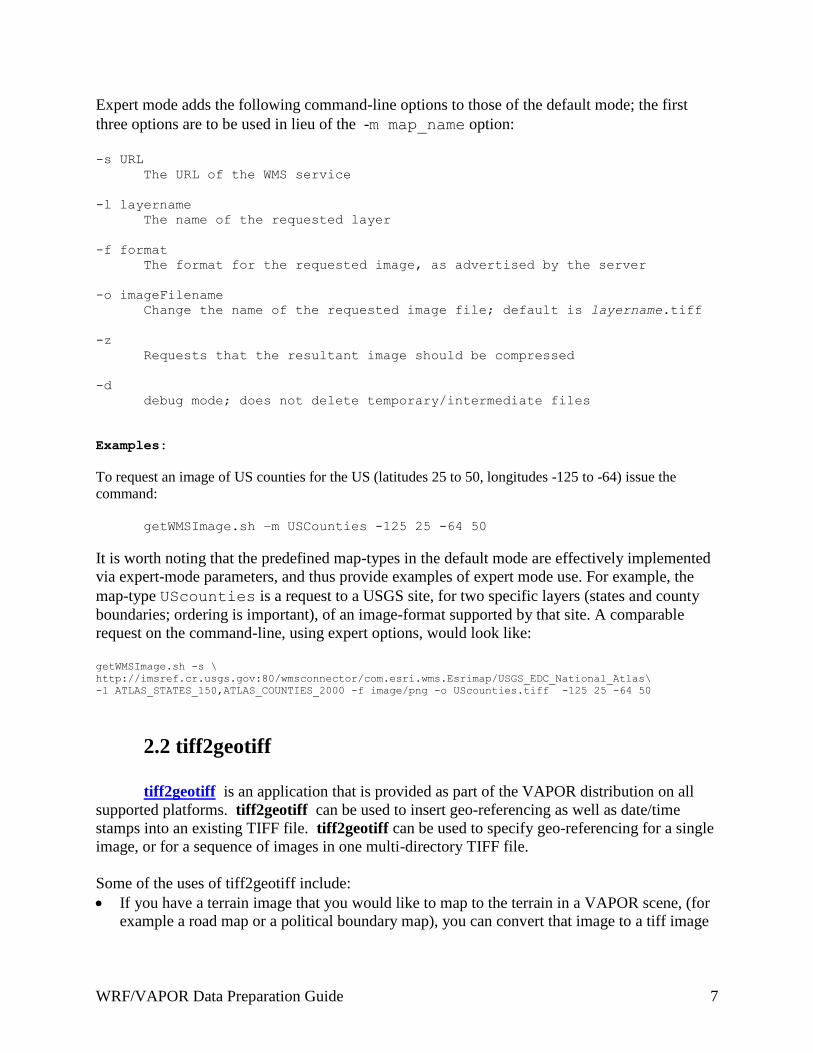
WRFVAPOR Data Preparation Guide 22
When geo-referencing is specified in the VDC geo-referenced images can be properly
positioned in the VAPOR scene LatitudeLongitude coordinates will also be displayed in the
Probe Region 2D View and Image panels