Vanden Hof Clipid

0005-1098(95)00094-l

Auromarica, Vol. 31, No. 12, pp. pp. 1751-1770, 1995 Copyright @ 1995 Elwier Science Ltd

Printed in Great Britain. All rights reserved ooo5-m9w5 $9.50 + 0.00

Identification and Control - Closed-loop Issues *

PAUL M. J. VAN DEN HOF t and RUUD J. P SCHRAMA +*

A survey is given of recent developments in iterative methods of closed-loop identljication and control design, where the ident$cation criteria are based

on control-relevant cost functions.

Kev Words-System identification; robust control; closed-loop identification; experiment-based control design; adaptive control.

Abstract- An overview is given of some current research ac- tivities on the design of high-performance controllers for plants with uncertain dynamics, based on approximate identification and model-based control design. In dealing with the interplay between system identification and robust control design, some recently developed iterative schemes are reviewed and special attention is given to aspects of approximate identification under closed-loop experimental conditions.

I. INTRODUCTION

The identification of dynamic models out of experimental data has very often been motivated and supported by the presumed ability to use the resulting models as a basis for model-based control design. As such, control design is considered an important intended-application area for identified models. On the other hand, model-based control design is built upon the assumption that a reliable model of the plant under consideration is available. Without a model, no model-based control design. These statements seem to point to two research areas between which one would expect many interrelations yet to exist. However reality is different.

In the past twenty years identification and control design have shown a development in two separate directions with hardly any relationships.

* Received 20 April 1994; revised 24 February 1995; received in final form 8 June 1995. The original version of this paper was presented at the 10th IFAC Symposium on System Identifica- tion, which was held in Copenhagen, Denmark, during 4-6 July 1994. The Published Proceedings of this IFAC meeting may be ordered from: Elsevier Science Limited, The Boulevard, Lang- ford Lane, Kidlington, Oxford OX5 IGB, U.K. This paper was recommended for publication in revised form by Guest Editors Torsten SGderstrGm and Karl Johan Astrom. Corresponding author Dr Paul M. J. Van den Hof. Tel. +31 15 2784509; Fax +31 15 2784717: E-mail [email protected]. + Mechanical Engineering Systems and Control Group, Delft University of Technology, Mekelweg 2, 2628 CD Delft, The Netherlands. * Now with Royal Dutch/Shell Group, NAM Business Unit Olie, PO. Box 33, 3100 AA Schiedam, The Netherlands.

While model-based control design has been developed into robust control, the importance of accurate model descriptions has been amplified. Apart from a nominal plant model, robust control- design methods employ a description of the model uncertainty, i.e. some (hard) upper bound on a specific mismatch between plant and model, in order to be able to evaluate robust stability and/or robust performance of the controlled plant, see e.g. Francis (1987), Maciejowski (1989) and Doyle et al. (1992). In the robust control-design paradigm, as a rule, one assumes model and uncertainty to be given a priori. However, one accepts that the (nominal) models that are used in general will not be able to capture all of the dynamics that are present in the plant, as exact modelling is either impossible or too costly.

In system identification, emphasis has long been on aspects of consistency and efficiency, related towards the reconstruction of the “real plant” that underlies the measurement data. However, in real- life situations, models that are identified from data will generally be contaminated with errors due to both aspects of bias (undermodelling) and variance. Even after the introduction of undermodelling issues in identification, as e.g. the asymptotic bias distribution expressions in prediction error methods in Wahlberg and Ljung (1986), it has still not been possible to formulate explicit results for the relia- bility (uncertainty) of identified approximate models. In this mainstream area of identfication, one mainly has to stick to asymptotic confidence inter- vals that are only valid in the case of consistent modelling see e.g. Ljung (1987). As a result there is a severe problem in explicitly quantifying the accuracy of estimated models.

At the end of the eighties it was pointed out by a number of people that the established techniques for identification and control design were hardly related to each other. This was due to two main points: firstly, it is generally not possible to bound

1751

1752 P. M. J. Van den Hof and R. J. I? Schrama

the uncertainty in identified models; and secondly, it is not clear what kind of (approximate) models are best suited for model-based control design.

Nevertheless, both communities would very likely agree on the relevance and importance of the question: “How can one arrive at appropriate (high performance) controlled plants on the basis of plant models that result from (or at least are validated by) measurement data?“.

The challenge to bring identification and control design more closely together and to tackle the problem formulated above, has led to a substantially increased attention for the problem area indicated by “identification for control” (from an identification point of view) or “experiment-based control design” (from a control-design point of view). The core of this problem is briefly indicated next.

Identification methods deliver a nominal model of a plant with unknown dynamics. Some methods deliver also an uncertainty region. The nominal model is just an approximation of the plant. Based on this nominal model, a controller has to be designed, assuming a certain level of accuracy (uncertainty) of the nominal model.

The performance achieved by this controller when applied to the plant will be highly dependent on the nominal model and the assumed uncertainty.

From here the research for control-relevant system identification branches into two directions. These directions are depicted in Fig. 1 which relates to the above remarks. The branch on the left illustrates the demand of robust control theory for a quantification of the “model error”. The right branch concerns the identification of a nominal model that is suited for high-performance control design.

In this paper we will emphasize the right branch of this problem, but without losing sight of the left branch. However, for a detailed discussion on methods and techniques for estimating model uncertainties, we will refer to the literature.

An interconnection between identification and control design has been investigated before. For example, in Astrom and Wittenmark (1971) probabilistic schemes for simultaneous identification and control design have been proposed, and in Gevers and Ljung (1986) an optimal identification experiment is proposed for control-design model applications. However, similar to the “classical” separation theorem in optimal control, these works consider exact models and aspects of approximation are not taken into account.

In this survey paper we will first elucidate the problem of concern, and we will briefly review the main approaches in the literature. In Section 3, we will present a framework for handling the problem

directed towards the matching of criteria that are used in control design and in identification. This leads to a generic form of iterative scheme of re- peated identification and control design. Next, in Section 4, we review recent developments in approximate closed-loop identification. Several examples of iterative schemes to solve the problem are presented and evaluated in Section 5, while final remarks conclude the paper.

2. MODELS FOR CONTROL - PRELIMINARIES

2.1. The high-performance control-design problem Let us first have a look at how model-based con-

trol design is commonly applied in practice. The basic ingredients are a set of control objectives, some nominal model, and possibly an upper bound on some model-plant mismatch (model error).

Let us denote with PO a linear, time-invariant plant, represented by its discrete-time transfer function; fi is a nominal model of that plant, and FA(!~, b) refers to an uncertainty set induced by the nominal model P and an uncertainty structure A, while the scalar b is a measure for the “size” of this set. The uncertainty set can for instance represent unstructured weighted additive uncertainty, as

?,,,(p, b) := {P I IP(eiW) - P(e’w)Ig(w)-l I b}(l)

with g( (u) some real-valued weighting function. We could also think of uncertainties in a multiplicative or structured form, see e.g. Doyle et al. (1992).

C will denote a linear time-invariant controller, and (PO, C) represents the closed-loop system composed of plant PO and controller C. We will employ the notion of performance of a controlled system in an abstract way, without having it specified in detail at this moment.

Given some 3 and PA (p, b), the robust control designer carefully chooses a control criterion and weighting functions, and calculates a controller by some numerical optimization. Next, the designer checks on the new controller by applying it to the nominal model p in order to examine e.g. the sensitivity, step response, robustness margins, etc. The designed controller will be accepted if it performs satisfactorily on the nominal model. If so, then the performance achieved for the plant is desired or even required to be similar to the designed nominal performance. Thus one pursues a high plant performance through a high nominal performance.

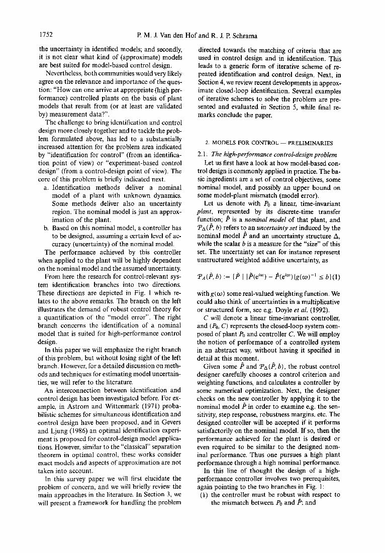
In this line of thought the design of a high- performance controller involves two prerequisites, again pointing to the two branches in Fig. 1: (1) the controller must be robust with respect to

the mismatch between PO and p; and

Identification and control - closed-loop issues 1753

Fig. I The two branches of control-relevant system identification.

(2) this mismatch must leave enough room to achieve a high performance.

The quantification of the mismatch between PO and P can, of course, be done in many different ways. It comes down to the specification of an uncertainty set CPA@, b) that contains (or is very likely to contain) PO. Many choices for the uncertainty structure A are possible: e.g. additive, multiplicative and coprime factor uncertainty in both unstructured and structured form; it is apparent that the achievable control performance for both p and PO is dependent on p, on A and on b. The fact that the achievable robust performance is limited for a given uncertainty set FA(& b) has been stated frequently in the control theory. However, from an identification point of view, the aim is to select a nominal model which does allow the above high-performance control design. Therefore, one can make the following converse observation.

The requirement of a high performance imposes limitations on the allowed structure and size of the uncertainty set ?A#, b), representing the mismatch between the plant and its nominal model.

For instance, it is well understood that a rea- sonable fit of the frequency responses around the crossover frequency of the control system is needed for robust performance, see e.g. Stein and Doyle- (1991). This is also illustrated by examples in e.g. Schrama (1992a), showing that a seemingly very accurate model in terms of its open-loop transfer function, may very well lead to a destabilizing controller. This supports the earlier statements con- cerning control-relevant model errors as put for-

ward by Skelton (1989), * who pointed out the need for iterative solutions to the modelling and control design problem. The example of Schrama (1992a) is sketched in the magnitude Bodeplot of Fig. 2, where an eight-order plant PO, is modelled by two fourth- order models, ti and 4. For frequencies smaller than 1.2 rad/s, PI cannot be distinguished from PO.

When using both models for model-based control design, aiming at a designed bandwidth of 15 rad/s, the controller based on pi will destabilize the model, whereas the controller based on & will achieve the designed performance. This is inspite of the model errors of 4 in the low frequency range. The higher accuracy of & around the designed bandwidth is the crucial thing here. Larger plant- model deviations are allowed at other frequencies, as long as they do not impair the control design. However the extent of the allowed deviations is un- clear without any knowledge of the controller yet to be designed. For more details on this example we refer to Schrama (1992a) and Schrama and Bosgra (1993).

2.2. Approaches in the literature

The growing interest for the interaction-area of system identification and robust control, has yielded different lines of research and different problem formulations that have been dealt with. Here we briefly summarize the main lines.

2.2.1. Quantzjication of model uncertainty . Here the reasoning is that in order to obtain iden-

* We acknowledge Michel Gevers for bringing this paper to our attention.

1754 P M. J. Van den Hof and R. J. P Schrama

Frequency [rad/sl

Fig. 2. Log-magnitudes of PO(-), A(- -), &(- . -),

tified models that are suitable as a basis for robust control design, one has to have available a measure for the model uncertainty, i.e. an upper bound on a mismatch between the plant and the identified model. Starting with assumptions on the class of systems that is feasible, and with assumptions on the class of disturbance signals that is considered to be realistic, one chooses a priori an uncertainty structure A. Additionally a model p is constructed and a bound b is derived such that the data and the prior assumptions provide evidence for the expression PO E PA@, b). Dependent on the type of disturbance signals that are considered, worst-case deterministic or stochastic, this expression becomes “hard” (with probability 1) or “soft” (with probability < 1). The type of priors that are chosen determine the type of results that are obtained. For a discussion on this phenomenon see Ljung et al. (1991) and Hjalmarsson (1993).

The worst-case deterministic type of problem has been addressed mainly in terms of frequency response data in Parker and Bitmead (1987), Helmic- ki et al. (1990) Helmicki et al. (1991), LaMaire et al. (199 l), Gu and Khargonekar (1992) Parting- ton (1991) and many others. They use uncertainty sets that allow for an expression like IIP- Poll o. < b. One generally does not achieve a minimization of this upper bound over a specified class of models, and the choice of nominal model d is just instru- mental in arriving at an upper bound of the plant- model mismatch. A more pragmatic approach to the problem directed towards curve-fitting of fre-

quency responses is presented in Hakvoort and Van den Hof (1994).

In the case of time-domain data, a deterministic/ worst-case approach with disturbance signals that are norm-bounded, is often referred to as set- membership identljication or - in a parametric setting - as parameter-bounding identification. Ac- counts are given in Fogel and Huang (1982), Nor- ton (1987) and Milanese and Vicino (1991). As in the previous situation, a (parametric) uncertainty structure A is chosen a priori and, based on the available data and prior assumptions, a parametric uncertainty set FA(fi, b) is derived, generally by parametric outer-bounding techniques. This area started off actually long before a connection was made with robust control. Originally it was directed towards the identification of poorly defined systems based on short data sequences. Several norms are used to outer-bound the obtained parametric uncertainty sets (as e.g. in terms of the transfer function magnitude, Wahlberg and Ljung (1992), 3&,-norms, Kosut et al. (1992) and Younce and Rohrs (1992), and f?t-norms, Makila (1991), Jacobson and Nett (1991) and Tse et al. (1993)). Direct outer-bounds on the frequency response of the model are considered in Hakvoort (1992) and Hakvoort (1993). Some important characteristics of this line of research are:

l due to the worst-case/deterministic character of the assumed disturbances, the obtained up per bounds on model errors will be very conservative if this worst-case disturbance does


not actually occur; l the worst-case disturbance signal will typically

be highly correlated with (“deliberately play- ing against”) the input signal;

. model uncertainty will generally not vanish as more data become available.

Approaches that consider disturbance signals to be stochastic, but that also account for undermodelling are given in Zhu (1989) Goodwin et al. (1992) Bayard (1992) and De Vries and Van den Hof (1995).

Model invalidation is another tool for quantifying model uncertainty. Given a set of priors on the data generating system and the type of disturbances, and a prior uncertainty set ?A@, b), it is verified whether measured data invalidates these prior assumptions. Accounts of this approach are given in Smith and Doyle (1992) and Poolla et al. (1994).

Critical and most interesting discussions on the item hard versus soft bounds (or equivalently worst- case versus stochastic noise) are provided in Hjal- marsson (1993) and Ninness (1993). For a general discussion on the problem of quantifying model uncertainty and worst-case identification we refer to the tutorial papers Ninness and Goodwin (1994) and Makila et al. (1994).

Note that in all approaches presented here the control design is not incorporated in the discussion. Control relevance of the identification methods is motivated by the fact that one needs to provide a (hard or soft) bound on a model-plant mismatch. Although the estimation of error bounds on the basis of experimental data has separate in- trinsic importance, by itself it is not sufficient for high-performance control design. This is caused by the fact that they are merely upper bounds of the uncertainty that are estimated. As uncertainty can be measured in many shapes and forms, the consequence of over-bounding the plant-model mismatch, and the consequence of chasing a specific uncertainty structure, for the resulting control performance should be taken into account. The key questions here are: which uncertainty structure to use and how to arrive at tight error bounds within this structure?

Whereas the achievable performance is of course limited by plant characteristics like (non)minimum- phase behaviour, and the ability of the plant to be modelled within a linear time-invariant framework, the achievable performance for an LTI plant with a model-based LTI controller, is additionally limited by the mismatch between PO and p, rather than by some upper bound.

2.2.2. Matching of ident@cation and control- design criteria A completely different problem is how to identify models that provide high-

performance controllers. This is the motivation for the second area, where most attention has been paid to the identification of nominal models that are suitable for high-performance control design, i.e. models that are accurate especially in those aspects that are essential for consecutive control design. Model-plant mismatches that are considered in the identification criterion have to be matched with the control-design objectives, and the considered uncertainty sets necessarily will become controller dependent. This has led to the construction of iterative schemes of identification, control design and renewal of experiments to obtain controlled plants that exhibit an improving control performance; controllers are tuned experi- mentally, based on a sequence of identified models. In the sequel of this survey we will specifically pay attention to this approach. Extended references can also be found in the Workshop Proceedings by Smith and Dahleh (1994), while the joint design of identification and control is very well advocated in the extended survey paper by Gevers (1993) and in the short survey by Bitmead (1993).

3. INTERPLAY BETWEEN IDENTIFICATION AND

CONTROL

3.1. System set-up

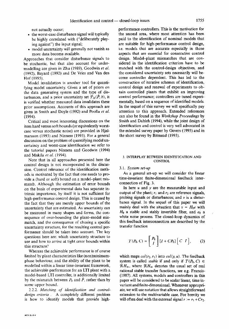
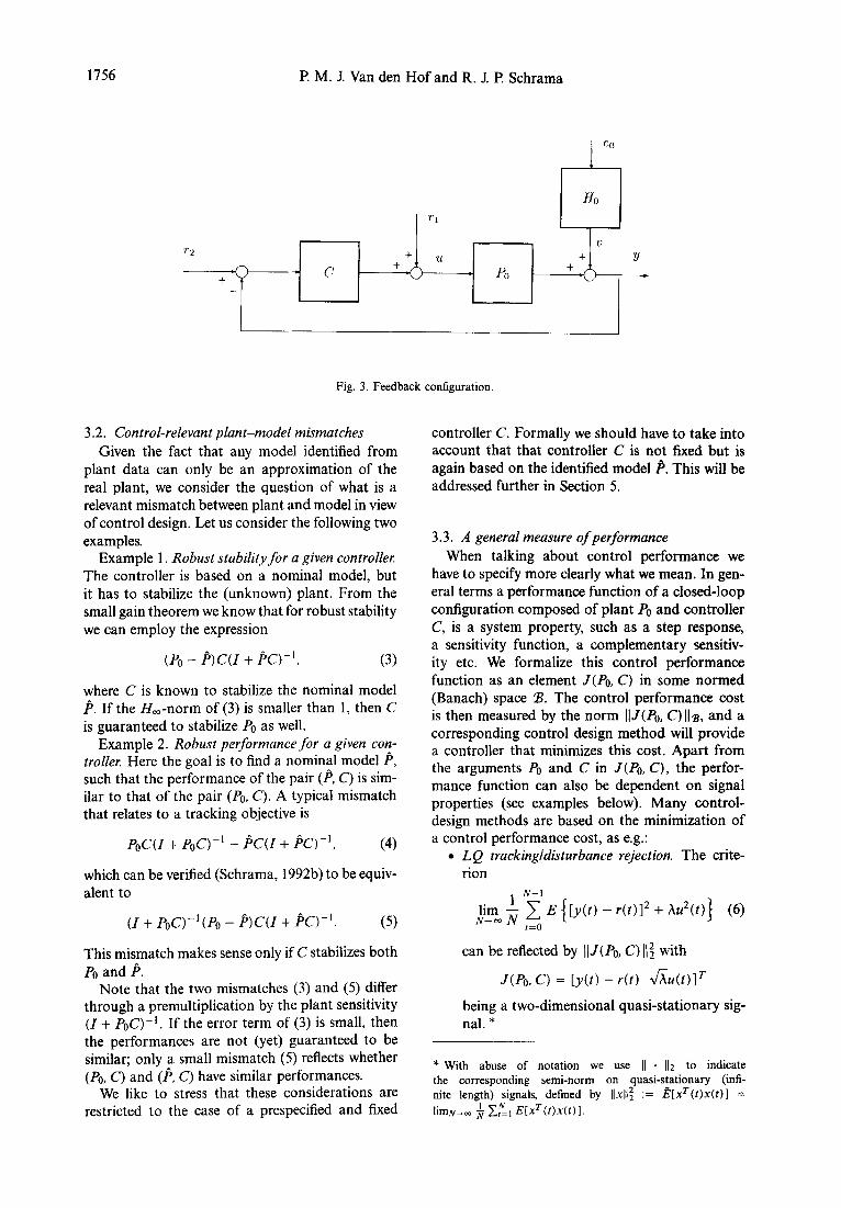
As a general set-up we will consider the linear time-invariant finite-dimensional feedback interconnection of Fig. 3.

In here u and y are the measurable input and output of the plant; rl and r2 are reference signals, probing signals or disturbances; and v is a disturbance signal. In the sequel of this paper we will mainly deal with the situation that v = Hoe with HO a stable and stably invertible filter, and es a white noise process. The closed-loop dynamics of this feedback interconnection are described by the transfer function

T(Po, C) = 7 [ 1 [I+CPol[C I], (2)

which maps col(r2, q) into col(y, u). The feedback system is called stable if and only if T(Po, C) E ZZH,, where RH, denotes the usual set of real rational stable transfer functions, see e.g. Francis- (1987). All systems, models and controllers in this paper will be considered to be scalar linear, time invariant and finite-dimensional. Whenever appropriate, we will use notation that allows straightforward extension to the multivariable case. For brevity we will often deal with the external signal r := rl +Crz.

1756 I? M. J. Van den Hof and R. J. I-? Schrama

e0

Ho r1

V 3

+ u + Y n

tY * c +A

v . PO +A

v

‘

Fig. 3. Feedback configuration.

3.2. Control-relevant plant-model mismatches Given the fact that any model identified from

plant data can only be an approximation of the real plant, we consider the question of what is a relevant mismatch between plant and model in view of control design. Let us consider the following two examples.

Example 1. Robust stability for a given controller. The controller is based on a nominal model, but it has to stabilize the (unknown) plant. From the small gain theorem we know that for robust stability we can employ the expression

(PO - B)C(Z + PC)_‘, (3)

where C is known to stabilize the nominal model P. If the ZZ,-norm of (3) is smaller than 1, then C is guaranteed to stabilize PO as well.

Example 2. Robust performance for a given controller. Here the goal is to find a nominal model p, such that the performance of the pair (Z? C) is similar to that of the pair (PO, C). A typical mismatch that relates to a tracking objective is

P&(Z + P()c)-’ - $C(Z + PC)_‘, (4)

which can be verified (Schrama, 1992b) to be equivalent to

(I + PoC)_‘(PO - B)C(Z + PC)-‘. (5)

This mismatch makes sense only if C stabilizes both PO and P.

Note that the two mismatches (3) and (5) differ through a premultiplication by the plant sensitivity (I + PoC)-~. If the error term of (3) is small, then the performances are not (yet) guaranteed to be similar; only a small mismatch (5) reflects whether (PO. C) and (p, C) have similar performances.

We like to stress that these considerations are restricted to the case of a prespecified and fixed

controller C. Formally we should have to take into account that that controller C is not fixed but is again based on the identified model P. This will be addressed further in Section 5.

3.3. A general measure of performance

When talking about control performance we have to specify more clearly what we mean. In general terms a performance function of a closed-loop configuration composed of plant PO and controller C, is a system property, such as a step response, a sensitivity function, a complementary sensitivity etc. We formalize this control performance function as an element J(Po, C) in some normed (Banach) space B. The control performance cost is then measured by the norm IIJ(Po, C)11~, and a corresponding control design method will provide a controller that minimizes this cost. Apart from the arguments PO and C in J(Po, C), the performance function can also be dependent on signal properties (see examples below). Many control- design methods are based on the minimization of a control performance cost, as e.g.:

l LQ tracking/disturbance rejection. The criterion

can be reflected by ((J(P0, C) 11: with

J(P0, C) = [y(t) - r(t) &(t)lT

being a two-dimensional quasi-stationary signal. *

* With abuse of notation we use II * 112 to indicate

the corresponding semi-norm on quasi-stationary (infi-

nite length) signals, defined by Ilxll~ := i?[xT(t)x(t)l = lim+ m $ c,“=, Erx~(r)xft)l.


l Mixed sensitivity optimization. The mixed sensitivity design is reflected by the choice

J(poJ c) = [ v, (I + P&y’

V2PoC(Z + P&)-’ 1 E 2W2’(7)

with weighting functions VI, V2 E 2ZH,, and the corresponding control performance cost

by IIJVo, C) Iloo. l H,-design based on robustness optimization.

This control-design scheme proposed by Mc- Farlane and Glover (1990) is reflected by the choice for

J(Po, C) = T(Po, C) E RHc2 (8)

with T(Po, C) as defined in (2). The corresponding control performance cost is

IIJ(P0, C)IIc0.

3.4. A link between iden@cation and control

Following the starting points as discussed in Sec- tion 2, the problem of concern is to identify a model P and to design a controller Cp such that the controlled model and the controlled plant both have a high performance. In other words we are look- ing for small values of ((J(Po, Cp) 11 and IIJ@, Cp) II, where the specific J and norm II . II are dictated by the control-design paradigm that is adopted. In this section we will not specify any choices for J and 1) . 1). When a pair (p, Cp) has been derived, it can be evaluated as a candidate solution to the joint problem of identification and control design by using the following triangle inequalities as considered by Schrama (1992a,b):

1 IL@, cp., II - lIJ(Po. Ck, - JCr’, Ck, II 1

5 IIJ(Po, cp, II (9) 5 IIJCP cfd II + IIJ(Po, cp., - J@, Cp,II.

In this triangle inequality we can distinguish:

IIJ(Po, Cp) II the achievedperformance,

llJ(p, Ck) 1) the designedperformance,

IIJ(Po, Cp) - JCP, Cp) (I the performance

degradation

This latter term is due to the fact that Cp has been designed from rj rather than from PO.

Taking as a starting point that we have to obtain a satisfying designed performance (if not we would not be willing to implement the controller on the plant), we can formulate two requirements to achieve a high-performance controlled plant:

IIJ(P, Cp) II is small, (10)

IIJ(P0, Cp) - J(B, Cp) II < llJ(P, Cp) [I.(1 1)

The requirement of (10) pertains to a high nominal performance. The strong inequality of (11) embodies the demand of a robust performance: if (11) is satisfied, then the difference between the designed performance function J(p, Cp) and the achieved performance function J(Po, Cp) is rela- tively small. Notice that the latter is not guaranteed by IIJ(Po, Cp) 11 = IV@, Cp) II, since these measures are aggregated quantities.

Standard methods for identification and control design can optimize either the model or the controller, each while the other element is fixed. However a simultaneous optimization cannot be obtained. This has led to the introduction of several iterative schemes directed towards the use of separate stages of identification and (model-based) control design, see e.g. Zang et al. (1991a,b), Hak- voort (1990), Anderson and Kosut (1991), Lee et al. (1992) and Schrama (1992a,b).

3.5. General form of iterative schemes

The basic principle behind the iterative schemes that have been proposed until now, is the explo- ration of the triangle inequality (9), in the sense that one aims at minimization of the right part (upper bound of the performance cost), by separate stages of minimization of either of the two terms (10) and (11). Simultaneous optimization of the upper bound (9) over both P and Ck is intractable by common identification and control-design techniques. Instead, separate optimization over d (identification) and over C (control design) is performed.

In general terms the model and the controller are obtained according to (indexes refer to step number in the iteration):

&+i = argmp IIJ(Po, Ci) - J(P, Ci) 11 (12)

Cj+i = argmin llJ(&+i, C) II c (13)

where p, C vary over appropriate model/controller classes, and in the control design one takes account of the constraint:

IIJ(pO, G+l) - Jt9+1, Ci+l)ll << llJt4+*, Ci+i)ll.(l4)

There are a couple of important observations to make here.

The identification criterion that is reflected in (12), is completely determined by the control performance function J(rt C) and the chosen norm 11 . /I, thus leading to a really control- oriented identification. The mismatch between plant and model is measured in terms of the control performance costs of plant and model, when controlled by the controller Cf. It is a nontrivial problem how to construct identification methods that achieve a criterion

1758 I? M. J. Van den Hof and R. J. I? Schrama

(12). Consider e.g. a weighted sensitivity as control performance function (i.e. (7) with Vi = V and V2 = 0). Then (12) simplifies to a norm on the weighted mismatch (5), i.e.

II VU + POW’(PO - P)CU + PC,-‘11, (15)

representing a nontrivial identification problem.

. As the control performance cost refers to a feedback connection of PO and Ci, the identification criterion (12) points to the use of measurement data from closed-loop experiments, in order to get information about J(P0, Co, (Schrama, 1992a).

l A newly designed controller Ci+ 1 will lead to a new performance degradation term (12) which in turn points to performing new identification experiments with this new controller Ci+i being implemented on the plant PO.

l The triangle inequality provides both an upper bound and a lower bound for the achieved performance, see (9). By making the performance degradation term small compared to llJ(p, Cr;)Il as in (1 l), the achieved performance is forced to be very close to the designed performance. In this way the control design is forced to provide a robust performance.

Generally design methods will yield their resulting controller through an unconstrained optimization: a criterion is minimized that incorporates some user-chosen weighting functions, reflecting the nominal performance level, as well as an indi- cation on the required robustness. However, there will generally not be a prior guarantee that the achieved robustness is satisfactory, i.e. whether (14) is satisfied. An additional robustness analysis of the designed controller has to certify this. This is also reflected in the (generic) block diagram of an iterative scheme of identification and control, as depicted in Fig. 4. If the robustness test is not passed satisfactorily, different actions may have to be taken as e.g.

. increasing the complexity (order) of the class of controllers considered;

. redesigning the weighting functions applied in the control design;

. identifying a more accurate (higher-order) model.

It has to be noted that in this discussion we have considered the control performance functions to be given a priori. To some extent this neglects the important choice of appropriate weighting functions as e.g. h in (6) and Vi, V2 in (7) that in normal practice are being designed (and redesigned) in the control-design stage.

In Section 5 we will take a closer look at different iterative schemes that have been elaborated in the

I experiments on (PO, C;)

i/o-data

.

identification

control design

robustness analysis

4

implementing (PO, C,+l)

I

Fig. 4. Iterative scheme of identification and control design.

past few years. They all show the basic components as discussed here, and mainly differ in the choice of the control performance cost and in the way the closed-loop identification is treated.

As we necessarily have to deal with identtica- tion of approximate models from closed-loop experiments, we will first review some results concem- ing approximate closed-loop identification. In that discussion we will limit attention to the prediction error identification framework.

4. APPROXIMATE IDENTIFICATION

4.1. “Classical” prediction error results

In a prediction error context, given input and output data of a plant to be modelled we determine the prediction error:

E(t, 8) = Hfq, W[yW - P(q, e4t)l (16)

with H( q, 8) the parametrized (output) noise model and P(q, 8) the parametrized input/output model,


8 running over some appropriate parameter space 0, while q is the forward shift operator.

The prediction error estimate (Ljung, 1987) is obtained by minimizing the squared sum of - possibly filtered - prediction errors:

N

i3~ = argrnn it; C s~(t, 0)* f=l

with ~(t, 8) = L(q)E(t, @, and L(q) some stable filter.

Under weak regularity conditions this prediction error estimate is known to converge with probability 1 to 0*, with

lT

8* = arg rn> & I

+t,(co)dw, (17) -7T

where in the open-loop case (C = 0): *

a EF = [ IPO - P(0) I*% + %] jg$ (18)

and au, aV are the spectral densities of input and noise, respectively. A so-called direct ident$cation in the closed-loop case with controller C (as in Fig. 3) yields a similar expression (17) with (see e.g. Gev- ers, 1993):

9 I ISOl EF = ISo[Po - fYe)112~r + -

Iswl*~’ 1 IL12 .-

IH(Q) (19)

where SO is the actual sensitivity (I + P&)-i and s(0) = (I + P(&C)-l is the sensitivity of the parametrized model.

by least-squares minimization of the prediction error E(t).

What we are aiming at is to find - based on signal measurements - a model P(8* ) that is obtained as the minimizing argument of an identification (approximation) criterion, that can be flexibly tuned, e.g. by appropriate choices of L and a,., to our needs in view of the control performance function. In order to achieve this, the criterion should not be dependent on the unknown noise spectrum

9”.

This alternative leads to a complicatedly parametrized model set, and as a result it is not attractive, although it provides us with an explicitly tunable approximation criterion, given by (17) with

Note that in the open-loop case, with a fixed noise model H(q, 0) = 1, as in the case of an output- error model structure, it can be verified that

e* = argm$i Il[& - P(B)]H,LJ(2, (20)

with H,, a (stable) spectral factor of au. In the closed-loop case it follows from (19) that

there does not exist a simple choice of noise model such that the +,-dependent term in (19) will become

Note that for validity of the asymptotic prediction error analysis leading to the above expression, the parameter set 0 has to be a connected subset of Rd being restricted to contain only models that generate stable predictors P(B) [ 1 + CP( 8)]-‘ .

In the next subsections we will present some recent developments in the area of closed-loop approximate identification, aiming at providing solutions to the problem sketched above.

4.2. Two-stage method

* For brevity the arguments eiO are suppressed in the frequency As an alternative method that can provide an domain expressions. explicitly tunable approximation criterion, a two-

independent of 8. As a result, the identification criterion (and thus the obtained model 4 will be es- sentially dependent on %, which is unknown. This is typical for “classical” closed-loop prediction error methods, see e.g. Soderstrom and Stoica (1989).

If open-loop techniques like (20) have to be used to obtain a control-relevant mismatch like e.g. (15) one can observe that input spectrum a,, and/or prefilter L have to be chosen dependent on the - unknown - plant PO and on the parametrized model p(e).

The closed-loop expression (19) nevertheless shows some clear resemblance with the desired approximation criterion (15) if we consider the first term in the expression (19). The weighting factor SO which is present in both expressions apparently is a weighting function that is obtained by performing the identification under closed-loop conditions. This is quite understandable if one realizes that it is exactly this sensitivity 5’0 that determines the relation between the external signal r and the input signal 24.

In an attempt to construct closed-loop approximate identification methods that have an explicitly tunable bias expression one can consider the following alternative. For simplicity we will assume the signal r to be available from measurements. If we know the controller C, one could consider a parametrized model P( 8), 0 E 0, and identify 0 through

dt, 8) = y(t) - p(e) r(t) I + p(e)c (21)

1760 I? M. J. Van den Hof and R. J. I? Schrama

stage identification method is proposed in Van den Hof and Schrama (1993).

The idea is that from closed-loop data one can first identify the plant sensitivity Sa as a black box transfer function S, using measured data (6 u}. Since u(t) = So(q)r(t) - C(q)&(q)v(t) and v and r are uncorrelated, this is an open-loop type of identification problem. In the second step of the procedure one identifies PO from:

y(t) = P(e)&(t) + E(t) (22)

with a,.(t) := $r(t) (23)

applying e.g. an output-error model structure in (22). The signal z.?,.(t) is simply constructed by the measured signal r and the estimate S being the result of the first step.

It can be shown that the approximation criterion in the second step of this procedure is determined by the spectrum

@‘EF = I [PO - fYQ)ISo + P(B)[So - s(B*)l I2 . @JLl*. (24)

In this expression B* is the (asymptotically) estimated parameter in the first step and L is a prefilter, filtering the prediction error in the second step. Note that when the first step is executed sufficiently accurately, i.e. S(fi*) - SO, then the expression above tends to a simple weighted additive mismatch PO -P, where the weighting incorporates the actual plant sensitivity SO. This has a clear resemblance with the robust control performance criterion (15).

4.3. Dual Youla parametrization The basic idea behind this method is introduced

by Hansen and Franklin (1988) in view of closed- loop experiment design. It was further elaborated and modified in Hansen et al. (1989), and also employed for approximate identification in Schrama (199 l), Schrama (1992b) and Anderson and Kosut (199 1). It utilizes the (dual) Youla parametrization of all plants that are stabilized by a given (known) controller. In order to describe this method, we need the following concepts.

Definition 1. (Vidyasagar (1985)). A linear, time- invariant, finite-dimensional plant P has a right coprime factorization (rcf) over X,H, if there exist N, D, X, Y E ZXH, such that P = ND-’ and XN + YD = I.Arcf(N, D)isnormalizedifN*N+D*D = I.

Through coprime factorizations a (possibly unstable) plant is represented by a quotient of two stable transfer functions. Coprimeness refers to the

property that the factorization does not exhibit can- celing terms that contain unstable zeros.

We can employ the following result from stability analysis.

Proposition 2. (Desoer et al. (1980)). Let C be a controller with rcf (N,, D,), and let Px with rcf (N,, 0,) be any system that is stabilized by C. Then the plant PO is stabilized by C if and only if there exists an R E RH, such that

PO = (N, + D,R)(D, -NCR)-!

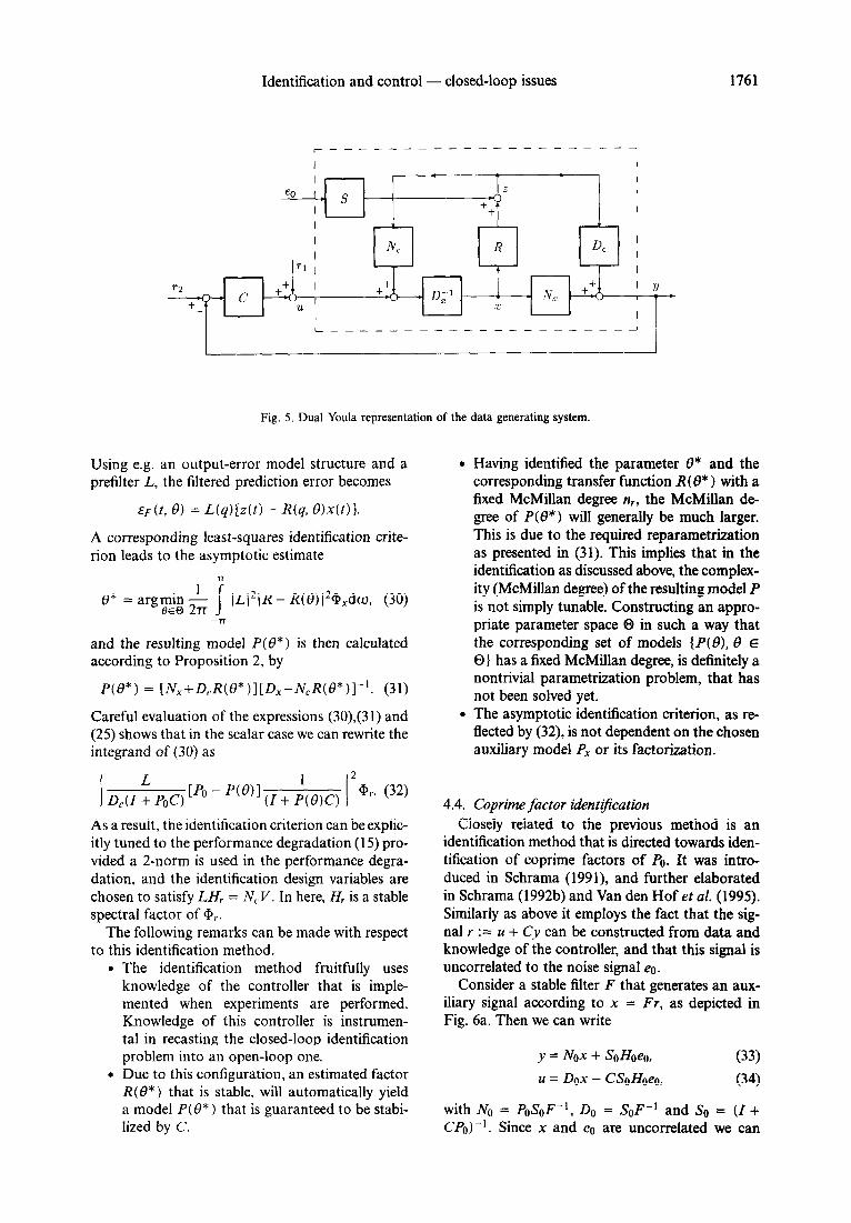
The above proposition shows a parametrization of the class of all plants that are stabilized by the given C. The parametrization is depicted in a block diagram in Fig. 5. Note that N,D;’ is just any (nominal, auxiliary) system that is stabilized by C. In the case of a stable controller C, a valid choice is given by N, = 0, D, = I.

Given the feedback configuration as presented in Fig. 3, it can be shown (Schrama, 1992b) that the unique value of R that corresponds to the real plant (PO) in this dual Youla parametrization is determined by

R = D,‘[Z + P&l-’ (PO - P,)D,, (25)

and that we can rewrite the noise contribution v(t) = Ho(q)eo(t) on the output, as in Fig. 3, into the form as indicated in Fig. 5 with

S = D;‘[I + PoC]-‘Ho. (26)

Now defining the signals z, x as indicated in Fig. 5 and writing the node equations x = D; * (U + Ncz) and y = NXx + Dcz, it follows that:

z = (D, + P,N,)-‘(y - Pxu), (27)

x = (D, + CN,)-‘(u + Cy, (28)

and

z = Rx + Sea. (2%

Moreover one can make the following observations: l the signals z and x can be reconstructed from

data through known filters, provided the controller C is known;

l signal x is uncorrelated with eo, as u + Cy = r1 + Cr2, and the external signals rl, r2 are assumed to be uncorrelated with eo.

This shows that we can identify a model 1; of PO through identification of R from reconstructed measurements {z, x} according to (29). Since x and eo are uncorrelated, the identification of R forms an open-loop identification problem. This implies that an approximate model of R can be obtained, where the asymptotic identification criterion is not dependent on the noise contribution on the data.


Fig. 5. Dual Youla representation of the data generating system

Using e.g. an output-error model structure and a prefilter L, the filtered prediction error becomes

~0, 0) = L(q)b(t) - Nq, OMt)l.

A corresponding least-squares identification criterion leads to the asymptotic estimate

IL)*)R - R(8) 1*9,dw, (30)

and the resulting model P(B*) is then calculated according to Proposition 2, by

P(0*) = [N,+D,.R(B*)][D,-N,R(B*)]-‘. (31)

Careful evaluation of the expressions (30),(3 1) and (25) shows that in the scalar case we can rewrite the integrand of (30) as

As a result, the identification criterion can be explicitly tuned to the performance degradation (15) provided a 2-norm is used in the performance degradation, and the identification design variables are chosen to satisfy LH, = N,.V. In here, H, is a stable spectral factor of cPV.

The following remarks can be made with respect to this identification method.

9 The identification method fruitfully uses knowledge of the controller that is implemented when experiments are performed. Knowledge of this controller is instrumen- tal in recasting the closed-loop identification problem into an open-loop one.

l Due to this configuration, an estimated factor R(f9*) that is stable, will automatically yield a model P(L)* ) that is guaranteed to be stabilized by C.

.

.

4.4.

Having identified the parameter 0* and the corresponding transfer function R( 8* ) with a fixed McMillan degree n,, the McMillan degree of IYe*) will generally be much larger. This is due to the required reparametrization as presented in (31). This implies that in the identification as discussed above, the complexity (McMillan degree) of the resulting model P is not simply tunable. Constructing an appropriate parameter space 0 in such a way that the corresponding set of models {P(O), 8 E 0) has a fixed McMillan degree, is definitely a nontrivial parametrization problem, that has not been solved yet. The asymptotic identification criterion, as reflected by (32), is not dependent on the chosen auxiliary model P, or its factorization.

Coprime factor identljkation

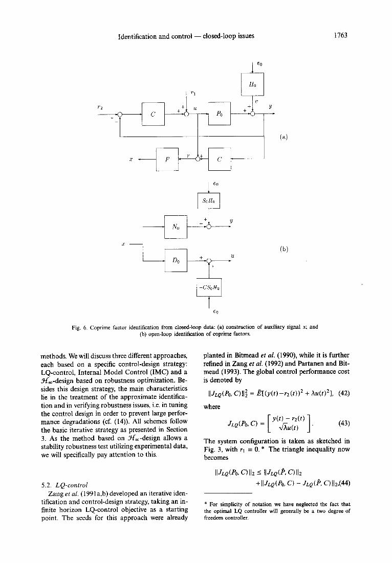
Closely related to the previous method is an identification method that is directed towards identification of coprime factors of PO. It was introduced in Schrama (1991), and further elaborated in Schrama (1992b) and Van den Hof et al. (1995). Similarly as above it employs the fact that the signal r := u + Cy can be constructed from data and knowledge of the controller, and that this signal is uncorrelated to the noise signal es.

Consider a stable filter F that generates an auxiliary signal according to x = Fr, as depicted in Fig. 6a. Then we can write

y = NOX + SoHoeo, (33)

u = DOX - CSoHoeo, (34)

with NO = P&F-‘, DO = SOF-’ and SO = (I + CPo)-I. Since x and eo are uncorrelated we can

1762 I? M. J. Van den Hof and R. J. l? Schrama

identify NO and DO in an open-loop way, thus utilizing the possibility of an explicitly tunable identification criterion. The plant model B is then constructed as B = N(&D(8)-‘.

Apparently there seems to be a lot of freedom in the choice of F. However this is limited if we restrict NO and DO to be stable and the signal x to be bounded, as is shown in Van den Hof et al. (1995):

Proposition 3. The filter F yields stable mappings (y, U) - x and x - (y, u) if and only if there exists an auxiliary system P, with rcf (NX, D,), stabilized by C, such that F = (D, + CNJ-*. For all such F the induced factorization PO = NOD;’ is right coprime. 0

This Proposition shows the clear resemblance of this scheme with the previous dual Youla parametrization. The choice of F as given in the Proposition shows that the resulting signal x matches the same signal in the previous section, cf.

(28). As in the previous method an intermediate signal

x is reconstructed from data (Fig. 6a). Next the two transfer functions between x and (y, U) are identified according to the scheme of Fig. 6b.

If we use a corresponding model structure

then a least-squares identification criterion will yield the asymptotic estimate determined by

(36)

According to (33) and (34) and the specific choice of F, the coprime plant factors that can be identified from closed-loop data satisfy

No

( )

=

Do (

PoU + CPo)-‘(I + CP,)D, (I + CPo)-’ (I + CP,)D, ) (37)

Now the question is how we can reformulate the identification criterion (36) into an expression in terms of PO and P(0) = N(B)D(e)-‘. If we would be able to construct a parametrization for N(B), D(e) that satisfies

[ ;f;] = [ p(e)u + cp(e)P

(z + cp(e))-~ ] U+ CPx)&W)

then the integrand expression in (36) can be written as

J IPo(Z + CPi$’ - P(8)(Z + CP(B))_’ 12IL, 12

+ IU + CPOP - (I + cP(e))-‘121Lz~2) Gp

(39)

The latter expression induces a very flexible approximation criterion in which clearly control-relevant mismatches can be recognized.

Note that the restriction to the parametrization (38) is nontrivial. A second remark is that the dynamics that are present in the coprime factors No, Do strongly depend on the choice of the auxiliary system P,. This also holds for the question of whether the factors can be accurately modelled by restricted complexity models. If both factors exhibit (very) high-order dynamics, then approximate identification of these factors may lead to an inaccurate plant model. This implies that somehow one has to get rid of the common dynamics in both factors, and thus also simplifying the parametrization restriction (38). In Van den Hof et al. (1995) an algorithm is presented in which the freedom in choosing P, is employed to arrive at coprime factors that are - nearly - normalized. This means that the factors (NO, DO) have minimal McMillan degree. It is achieved through a similar strategy as in the two-stage method, described earlier. First an accurate - high-order - estimate is made of NO and DO; the resulting coprime factors are normalized in a normalization procedure, and these latter factors are subsequently used as an auxiliary model. The factors NO and Do that result from this choice of P, and D, will be almost normalized (in the sense that N”N + D* D - I), and can be accurately identified by using a model structure for N(B), D(e), given by

N(0) = b(q-‘, @_f(q-‘, Q)-l, (40)

D(Q) = a(q-‘, W-(q-l, @-‘, (41)

with a, b and f polynomials of specified degree. This parametrization now approximately satisfies the restrictions of (38). Moreover it guarantees that the McMillan degree of the resulting plant model is equal to the McMillan degree of the estimated coprime factors.

As a final note we remark that due to this coprime factor framework the identification methods discussed in the previous Sections 4.3 and 4.4 do not meet any problems in handling unstable plants and/or unstable controllers.

5. ITERATIVE SCHEMES UNDER CONSTRUCTION

5.1. Introduction While in the previous section we discussed the

developments in approximate closed-loop identification, we will now return to the interaction with the control design, by addressing several iterative


e0

Ho 7-1

2)

r2 + u + Y A

+A +

+Y - c ” * PO ”

_

e0

So Ho

+ + Y

- No v

X-

(b) U

c Do +

-C&Ho

I e0

Fig. 6. Coprime factor identification from closed-loop data: (a) construction of auxiliary signal x; and (b) open-loop identification of coprime factors.

methods. We will discuss three different approaches, each based on a specific control-design strategy: LQ-control, Internal Model Control (IMC) and a Hm-design based on robustness optimization. Be- sides this design strategy, the main characteristics lie in the treatment of the approximate identification and in verifying robustness issues, i.e. in tuning the control design in order to prevent large performance degradations (cf. (14)). All schemes follow the basic iterative strategy as presented in Section 3. As the method based on Hm-design allows a stability robustness test utilizing experimental data, we will specifically pay attention to this.

5.2. LQ-control

Zang et al. (I 99 1 a,b) developed an iterative identification and control-design strategy, taking an in- finite horizon LQ-control objective as a starting point. The seeds for this approach were already

planted in Bitmead et al. (1990), while it is further refined in Zang et al. (1992) and Partanen and Bit- mead (1993). The global control performance cost is denoted by

hQ(~O, C,i; = 8[b’(t)-r2W2 + h&)*1> (42)

where

The system configuration is taken as sketched in Fig. 3, with ri = 0. * The triangle inequality now becomes

IIJLQ(pO> c) 112 5 ikQ(p, c) 112

+IIJLQ(h c) - &Q(k c) 112444)

* For simplicity of notation we have neglected the fact that the optimal LQ controller will generally be a two degree of freedom controller.

1764 I? M. J. Van den Hof and R. J. P, Schrama

where JLQ @, C) = I

y,(t) - f-20)

A~,,(~) ) and am, 1

The LQ controller is obtained by minimizing the performance cost &.,

uc(t) the corresponding output/inpu< signal in the design loop, i.e.

yc = F&r2 + SAel, (45)

uc = 532 - CSAel. (46)

In this expression ,? and fi denote the sensitivity function of the i/o model 3 and the estimated noise model, respectively. The signal ei is the assumed noise signal in the design loop.

Through careful evaluation of the performance degradation term, JLQ(Po, C) -JLQ(P, C), it follows that the (squared) norm of this term becomes

B[(y(t) - Y,W2 + A(u(t) - ~c(~)~21. (47)

This is the related identification criterion that is induced by (42). In order to come to an identification set-up in which this criterion is minimized, (47) can be rewritten as

1 lT

G l{ Iso~o12(l + hlC12)@~”

-7T

+ICSo[Po - PWlS(0)12(1 + hlC12)9,,) dco.

(48)

In this latter derivation, Zang et al. (1991b), have taken ei = 0. As an identification set-up, it is proposed to apply a direct-type closed-loop prediction error criterion conformable to (19) with r := C(q)r2, with a fixed noise model H(q, 8) = 1 and a prefilter L satisfying

1 + NCl2 ILWI~ = (1 + wmswl2 = II + cptej12.

(49)

Such a choice of L makes the closed-loop identification criterion (17) and (19) equivalent to (48). (Note that we may neglect the e-independent terms in the integrands.) A remaining problem is the fact that this optimal prefilter is again a function of the unknown parameter 8, which implies that the required model structure is not a regular output-error model structure. An “approximate” solution is provided by using the model estimate from the previous step in the iteration, i.e. L(8) = L( 8i-1). In this way the prefilter becomes fixed, but the two criteria (17) and (19) and (48) no longer match exactly.

Remark 4. A similar approach to the identification problem is taken in Hakvoort (1990) and Hakvoort et al. (1994). There, the design loop is chosen to be contaminated by the same noise eo as in the achieved loop. For that case the same choice of optimal prefilter L( 8) (49) is obtained, and conditions are given for which a choice L( 8) = L( Bi-1) provides equivalent criteria (17),(19) and (48).

IIJLQP, C) II; = i?[(y,(t) - r2(t)J2 + hu,.(t)21. (50)

This design strategy does not account for any mismatch between the nominal model and the actual plant. This implies that during the control design we have to verify whether (14) is satisfied. Only under this condition can one guarantee that the achieved performance will be similar to the designed one. Zang et al. (1991 b) propose a local design criterion that accounts for this mismatch. This local design criterion should prevent a decreasing designed (nominal) performance cost which would dramati- cally increase the performance degradation cost. It takes the form of

IIJLQ,~~~~~~(~, C)llz = ~{[Fl(q)(yAt) - r2(t))12

+ m~qMN2~~ (51)

with Fi (eiW) = l/2

, F2(eiW) =

The spectra in this expression are estimated on the basis of measurement data from the actual system and of simulation data from the designed loop.

Recent contributions to this iterative scheme are presented in Zang et al. (1995).

5.3. Internal Model Control (IMC)

In Lee et al. (1992), Lee et al. (1993a) and Lee et al. (1993b) an iterative scheme of identification and control design is proposed based upon the internal model control (IMC) design paradigm. The resulting iterative scheme is often indicated as the “windsurfer approach” * (Anderson and Kosut, 1991), referring to the presumed iterative way that people take when learning windsurfing: starting with a control system with moderate bandwidth, while ex- perimentally refining the model and increasing the bandwidth of the controlled “plant”.

The control performance is based on

pot JIMCU’O, Cl = - - 1 +P&

Ti. (52)

with JIMC E RH,, Td is some prechosen desired complementary sensitivity, and the performance cost is taken to be the 3fm-norm of J,Mc. Td is chosen to be of the form ( & jn+’ , with h E a the closed-loop bandwidth, and n a prechosen integer.

The choice of control performance cost induces the performance degradation

II JIMCU’O, C) - JIM& 0 Ilo

* Due to local climate conditions this term is not so often used by the north-west European iterators.

Identification and control - closed-loop issues A

=((poc_ 1 + P&

+llm. (53)

1765

C = argm$n IIT/T($, c)Wlloo. (55)

The mismatch between complementary sensitivity functions has already been shown to be a control- relevant plant-model mismatch, see e.g. (4) and (5). In Lee et al. (1992) the closed-loop identification scheme based on the dual Youla parametrization is employed to identify a stable transfer function R, as described in Section 4.3 and equation (29). By choosing a least-squares prediction error criterion with a prefilter L = A’,., the resulting parameter estimate will converge to (assuming +,- z 1)

Tr

0* = argmjn I

I* - 0

1 ~~;&12dw. (54) --TT

where the plant model P( 6) is parametrized according to (3 1). In this setting the tim-norm of the performance degradation is replaced by the 2-norm of the least-squares prediction error criterion. Due to the parametrization (3 1) the estimated plant model will generally be of high order; a subsequent model- reduction procedure based on frequency-weighted balanced reduction, conformable to (53) is applied to keep control over the model order of P and the resulting order of the controller.

The control design uses IMC-design techniques for a nominal design that achieves the predesigned closed-loop bandwidth. During the iterations of identification and control design, the nominal closed-loop bandwidth h is gradually increased as the identified model becomes more accurate around and beyond the designed closed-loop bandwidth. When increasing h for a specific model Ii, the performance degradation is monitored through step response experiments on the achieved and designed loop. When the responses are different, this indicates either the limit of validity of the current model Pi, and thus the need for a new model Pi+,, or the limits of performance that can be achieved. In Lee et al. (1993b). considerations of variance of the model estimates are also gathered into the iterative scheme. While the original method has been worked out for stable plants and stable controllers only, a further extension to the handling of unstable plants is presented in Lee (1994).

5.4. H,-design based on robustness optimization III the work of Schrama (1992a,b), Schrama

and Van den Hof (1992) and Schrama and Bosgra (1993) an iterative scheme of identification and control design is elaborated, utilizing the robust control-design method of Bongers and Bosgra- (1990) and McFarlane and Glover (1990). The control-design criterion is:

T(p, C) is the 2 x 2 transfer matrix as defined in (2) that embodies all feedback properties of the closed- loop system, including disturbance and noise at- tenuation, sensitivity and robustness margins, and with V and W appropriate stable weighting functions. Through specific choices of I’ and W this method reduces to specific methods like weighted- sensitivity minimization or mixed-sensitivity minimization (see also Section 3.3).

For V = W = I, the following robustness result is known from Glover and McFarlane (1989) and Bongers and Bosgra (1990).

Proposition 5. Let T(p, C) be stable, and let ($,,, fi,) be a normalized rcf of P. Define the uncertainty set PA@, y) := {PA = (& + AiV)(b, +

AD)-‘, ;; /I II

< y). Then ah plants in FA@, y)

are stabilized by C if and only if II T(k C) Ilm I ‘y-1. cl

As the control design amounts to minimizing II T(?, C) Iloo this corresponds to a maximization of the stability robustness margin with respect to (stable) perturbations of normalized rcfs of the plant model. Additionally the resulting controller pursues some traditional control objectives like a small sensitivity at the lower frequencies and a small complementary sensitivity at the higher frequencies. The bandwidth of the designed loop will be close to the crossover frequency of the nominal model P. This controller is also known to optimize the stability robustness margin in the sense of the gap metric, see Bongers and Bosgra (1990) and Georgiou and Smith (1990).

In the given situation the control performance function is defined by

JRO(pO,c) = TU'o, c), (56)

while its cost is measured as the corresponding 3&,- norm. The induced performance degradation becomes

II TWO, C) - TCt C) Ilm. (57)

It can simply be verified that this performance degradation is an extended version of the degradation (53) in the case of the IMC design.

5.4.1. Zden tification . The identification method has to provide a model p that (asymptotically) minimizes the performance degradation (57). In the proposed iterative scheme an identification criterion is chosen that equals II T(Po, C) - T(j, C)llz, where minimization of the 2-norm is used to obtain a reduction of the co-norm of the corresponding mismatch. This replacement is justified by the

1766 F? M. J. Van den

fact that an accurate &-approximation implies an accurate L,-approximation, provided that the error term is sufficiently smooth and small, see e.g. Caines and Baykal-Gtirsoy (1989). Identification of P = argminp II T(Po, C) - T@‘, C) 112 is obtained by applying the coprime factor identification as described in Section 4.4. Under the parametrization restriction (38) it can be verified that

TWO, Cl - TV(Q), C)

(58)

Minimization of the 2-norm of this expression can be achieved through least-squares identification as in (36) with L, = L2 = L, satisfying IL12@,. = 1 + I C12. In the first versions of this iterative scheme, the identification was actually performed based on frequency response data of the plant. Later exten- sions in Van den Hof et al. (1995) also show the use of time-domain data.

54.2. Control performance enhancement . The controller C of (55) with I/ = W = I depends solely on the nominal model p. As a result the achieved performance II T(Po, C) II to may be substantially different from the designed performance IIT& C)llw. In order to preclude large performance degradations the nominal control design is furnished with weighting functions. Like in McFar- lane and Glover (1990) this iterative scheme uses just a simple scalar weight, W-’ = V = diag(or, I), leading to the control design

C = argmin IIT(d, z)II,. ?

(59)

The resulting controller yields optimal robustness for H,-bounded perturbations of normalized rcf s of the weighted model c&. Additionally, the bandwidth of the feedback system will be around the crossover frequency of otp. When the frequency response of the nominal model p rolls off in the range where I &(eiw) I - 1, one can push out the designed bandwidth by increasing the weight o(, thus allow- ing more control action. In other words, a large a corresponds to a high nominal performance.

Note that the introduction of this weighting does not hinder the identification part, as it simply acts as a scalar weight on i), PO and C.

At each control-design step the weight o( is increased just gradually in order to enhance the nominal performance, while the performance degradation has to remain acceptably small. This implies that at iteration step i, having available pi+,, O(~, Ci, a choice is made for ai+i > c+ requiring that

Hof and R. J. I? Schrama

G+l IIT(ai+Po, - ai+l ) - T(ai+l&+l, o(i+l Ci+l ) II

m

<< IIT(aj+l&):+l, (60)

while the sum of left- and right-hand expression has to remain sufficiently small.

The right-hand side of (60) is actually minimized in the control design and thus can be calculated simply. The left-hand side is not directly available, as experiments with the new controller Cj+i are not yet available. From the identification in step i we have obtained knowledge of

G IIT(%Po. F) - T(cx#~+~, ~)ll,. (61) I I which is clearly different from the left-hand side of (60). In the proposed iterative scheme a high-order frequency response estimate of PO is employed in order to estimate this left-hand side of (60) for each new candidate ai+ 1.

5.4.3. Robust stability analysis . Having selected ar+i and calculated Cj+i, there is no formal guarantee that the plant PO is stabilized by Ci+i. This is due to the fact that the design (55) is an unconstrained optimization; although the robustness is optimized, there is no prior guarantee about the extent of the robustness margin. Moreover, (60) can be verified only by replacing PO by some estimate of PO.

In order to test the robust stability before actually implementing the newly-designed controller, we can exploit a robust stability result that utilizes an uncertainty structure on (coprime factors of) Pj+*

that is controller dependent.

Proposition 6. (Schrama (1992b).) Let controller Cr stabilize both the mode1 fii+i and the plant PO. Let c~+ i&+i have a normalized rcf (fin, &,> and let cxz,Ci have a normalized rcf (IV,, D,). Let O(r+iPo have an rcf (NO, DO) that satisfies NO = fi + AN and DO = b + AD, with IlLAN AD] (lm < y. Then PO is stabilized by Ci+i if

L 1 ll[~i+lDn +- G+lNnl-‘[G+1 - GlDcIIw < Y- ‘. (62)

This result is based on a Youla parametrization for both the controller Ci+i and the plant PO. The resulting stability test is non-conservative in the case Ci+i = Ci, as in that case it matches with the Youla parametrization. Note that the left-hand side of (62) is completely known. This stability test calls for identification methods that provide a 3f--error bound on the normalized rcf of the weighted model ai+ iPi+i. Once an upper bound y can be found from data, (62) can be verified. In Schrama (1992b) high-order frequency domain estimates of PO are taken to construct the required error bounds and to verify robust stability.


5.5. Other approaches

Apart from the three methods presented in this section so far, there are a couple of alternatives that all incorporate iterations between model identification and control design.

In Liu and Skelton (1990) an iterative method is presented that relies on closed-loop impulse response experiments for identifying a model using the q-Markov cover theory; the model matches the first sequence of Markov parameters and the first elements of the output covariance function of the closed-loop plant. An open-loop model is reconstructed by employing knowledge of the controller and through application of a model reduction technique. This identification is iterated with a control- design scheme that minimizes the control energy of the closed loop subjected to inequality constraints on the output variance.

In Astrom (1993) considerations are given for the matching of criteria in identification and control. For several control-design strategies the relevance of least-squares identification in closed loop using appropriate data filters is discussed. This leads to results that are in line with the ones obtained for LQ-control as discussed in Section 5.2.

In Graebe et al. (1993) and Graebe and Good- win (1993) an iterative scheme is proposed that is based on closed-loop identification of multiphca- tive model increments, a stochastic embedding approach for quantifying the model uncertainty and an IMC control-design method. With each iteration the model complexity is increased so as to capture more of the relevant plant dynamics in the model. Due to the model uncertainty quantification a bandwidth of robust performance can be pre- dicted at each iteration.

In a number of approaches one does not explicitly use closed-loop experiments. Bayard et al. (1992) matches the identification and control design for a mixed sensitivity type of control design, where the actual identification is replaced by a control-relevant weighted curve fit on the frequency response of the (noiseless) plant. In Rivera et al. (1992), considering several control objectives, an account is given on the construction of control- relevant prefilters to be applied in open-loop identification in order to arrive at control-relevant models. Shook et al. (1992) propose data prefilters in order to provide an identification criterion that matches a generalized predictive control criterion; this method is worked out for a noise-free situation.

5.6. Evaluation

Despite their differences, the iterative schemes presented in the previous subsections find their roots in a similar philosophy to the problem, for

which a generic formulation has been given in Section 3. Basic features are:

l An appropriate nominal model is indispens- able for achieving a high performance controlled plant.

l Approximate identification in closed loop serves to match the achieved and designed performance as close as possible.

l Generally the iterative algorithms start off with a moderate nominal performance requirement (loose controller) and pursue a nominal performance improvement by gradually increasing the nominal performance requirement (cf. increasing designed bandwidth in the IMC-design and increasing o( in the robustness optimization of Section 5.4).

l Decision points occur whenever one is no longer able to achieve a performance degradation cost that is (far) lower than the designed performance cost. In that situation one either has to increase the complexity of the model (to reduce the performance degradation) or to increase the complexity of the controller (to reduce the nominal performance cost), or to realize that one may have reached the limits of achievable performance.

l Convergence of the iterative schemes is obtained through monitoring the iterations, rather than by formal theoretical justification.

The approach that is present in these iterative schemes can be viewed as a means of letting experiments reveal what control performance can be achieved for the plant under consideration. In this way one can “learn” about the achievable plant performance as the iterations go by, by succes- sively retuning the controller based on information obtained from experiments. Referring back to the problem as stated in the introduction of this paper, the surveyed area offers a clear approach to the goal of arriving at appropriate controlled plants on the basis of experiment-based plant models. How- ever, we are not yet in a situation in which full an- swers are provided, and many questions remain to be solved. We list only a few of the open problems.

l Attention is focused to bias aspects of the identified models, rather than to variance aspects. A recent contribution that supports the approach presented here and that focuses on variance aspects in the considered identification setting, is given in Hjalmarsson et al. (1994a).

l Attention is restricted to classical prediction error methods leading to the use of 3-&norms in model approximation, while actually from a point of view of control performance cost an 3& criterion would be most suitable; see e.g. the methods in Sections 5.3 and 5.4. This

1768 l? M. J. Van den Hof and R. J. P. Schrama

mismatch of norms requires attention in future research, and may lead to the explicit use of 3-1,~norms in identification procedures.

l The possible convergence of these schemes has to be further analysed, and conditions have to be formulated for avoiding divergent behaviour.

l The prediction of performance degradation every time a new controller is designed calls for the explicit use of uncertainty models. This point refers to the problem of satisfying (14) after a controller redesign. In this uncertainty modelling, uncertainty structures have to be used that are specifically suited for the considered control performance cost, in the sense that non-conservative statements can be made with respect to the left-hand side of (14).

One can argue whether one needs closed-loop experiments and closed-loop identification in order to obtain identified models that serve our goal. As apparent in the analysis of this paper, performing the identification in closed loop provides a weighting of the identification criterion that can exactly support the intended control application of the model. The controller shapes the input of the plant to a form that stresses those components that are control relevant. The experimental situation under which models are obtained is closely matched to the experimental situation in which the model and its induced controller, have to perform particularly well. A similar situation can be approximated by open- loop identification employing weighting functions (prefilters) that are plant and controller dependent. Consequently, that similarity can only be approxi- mative.

The presented iterative ways of increasing the plant performance are specifically directed towards situations in which the achievable plant performance is not known a priori. In the case in which one knows that a specific (moderate) plant performance can be obtained and which control-design weights have to be used, it may not be too hard to find appropriate prefilters in open-loop identification, that will provide a model that supports the required control design.

When arriving at a model that is suited for high- performance control, one is not automatically as- sured of an overall accurate open-loop model. It has been shown in a number of situations that one can easily arrive at high-performance control SYS-

terns with only a moderate, or even a bad, open- loop performance of the nominal model, see e.g. Zang et al. (1991a) and Schrama (1992a) as also illustrated in Section 2. If one additionally wishes a model that satisfies the experimenter’s prior knowledge or that is an accurate open-loop description of the plant, this will have to be considered as an addi-

tional model requirement, for which a price has to be paid, generally in terms of a higher model order and/or more experiments.

We also would like to point to the “inner” iterative loop that is present in the block diagram in Fig. 4. Especially in situations where experiments are expensive and time consuming, it can be advan- tageous to fully exploit the possibilities of this “inner” loop, i.e. repeating identification and control design without renewing the experiments.

We have focused on the problem of arriving at well-controlled plants by separate though related stages of model identification and model-based control design. An interesting account of a direct controller tuning based on experimental data is given in Hjalmarsson et al. (1994b).

Successful real-life applications of high-performance control design will have to be the ultimate justification for the methods presented in this survey. While most of the techniques presented here are supported by simulation examples, it is gratifying that also a couple of real-life applications have already been reported. The iterative scheme of Zang and co-workers with LQ control has been applied to a sugar crane crushing mill, see Partanen and- Bitmead (1995) while the scheme of Schrama and co-workers with the Hm-design has been applied to a servomechanical system in Schrama and Bos- gra (1993). One single step in this latter scheme has also been applied to the pick-up mechanism in a Compact Disc player, see De Callafon et al. (1994).

6. FINAL REMARKS

In this paper we have reviewed some aspects of the research related to the problem of designing a high-performance controller for a plant with unknown dynamics through separate identification and control design. The underlying ideas in this area are quite close to adaptive control. Whereas in adaptive control the procedures of identification and control design are completely intertwined, the approaches discussed here attempt to provide a separate analysis of both steps, and to accomplish a joint performance criterion of both parts.

Iterative procedures in which the performance level of the controlled plant is gradually increased are actually quite appealing. In engineering practice a product is commonly accomplished by a number of successive improvements rather than by a one- step design that starts from scratch. Why should control engineering be different? The implication of this is that one should not focus on an ideal but possibly unachievable desired control performance. Instead one better aims at an improvement of the performance that has already been achieved.


Acknowledgements- The authors gratefully acknowledge their colleagues at Delft University of Technology for fruitful discussions and their contributions to this work.

REFERENCES

Anderson, B. D. 0. and R. L. Kosut (1991). Adaptive robust control: on-line learning. In Proc. 30th IEEE Con& Decision

and Control, Brighton, U.K., pp. 297-298. Astrom, K. J. (1993). Matching criteria for identification and

control. In Proc. 2nd European Control Con$, Groningen, The Netherlands, pp. 248-251.

Astrom, K. J. and B. Wittemnark (1971). Problems of identification and control. _? Math. Anal. & Applic., 34, 90-l 13.

Bayard, D. S. (1992). Statistical plant set estimation using Schroeder-phased multisinusoidal input design. In Proc. Am.

Control Conf, Chicago, IL, pp. 2988-2995. Bayard, D. S., Y. Yam and E. Mettler (1992). A criterion for

joint optimization of identification and robust control. IEEE

Trans. Autom. Control, AC-37, 986-991.

Bitmead, R. R., M. Gevers and V Wertz (1990). Adaptive

Optimal Control, The Thinking Man’s GPC. Prentice-Hall, Englewood ClitTs, NJ.

Bitmead, R. R. (1993). Iterative control-design approaches In Preprint 12th IFAC World Congress, Sydney, Australia, 9, pp. 381-384.

Bangers P M. M. and 0. H. Bosgra (1990). Low order robust 3f- controller synthesis. Proc. 29th IEEE Conf Decision

and Control, Honolulu, HI, pp. 194-199. Cainea P E. and M. Baykal-Giirsoy (1989). On the Lm con-

sistency of L2 estimators. Syst. Control Letters, 12, 71-76. De Callafon, R. A., P. M. J. Van den Hof and D. K. de Vries

(1994). Identification and control of a compact disc mechanism using fractional representations In Preprint 1Oth IFAC Symp. on System Identi$cation, 4-6 July 1994, Copenhagen, Denmark, Vol. 2, pp. 121-126.

Desoer, C. A., R. W. Liu, J. Murray and R. Saeks (1980). Feed- back system design: the fractional representation approach to analysis and synthesis. IEEE Trans. Autom. Control, AC- 25, 399412.

De Vries D. K. and P. M. J. Van den Hof (1995). Quantifica- tion of uncertainty in transfer function estimation: a mixed deterministic-probabilistic approach. Automatica, 31, 543-

557.

Doyle, J. C., B. A. Francis and A. R. Tannenbaum (1992). Feedback Cor:tml Theory. MacMillan, New York.

Fogel, E. and Y. E Huang (1982). On the value of information in system identification - bounded noise case.. Automatica,

l&229-238. Francis, B. A. (1987). A Course in 3f- Control Theory.

Springer, Berlin. Georgiou, T T. and M. C. Smith (1990). Optimal robustness in

the gap metric. IEEE Trans. Autom. Control, AC-35, 673-

686.

Gevers, M. and L. Ljung (1986). Optimal experiment design with respect to the intended model application. Automatica, 22, 543-554.

Gevers, M. (1993). Towards a joint design of identification and control? In H. L. Trentelman and J. C. Willems (Eds), Essays

on Control: Perspectives k the Theory and its Applications. Birkhauser, Boston, pp. 111-151.

Goodwin, G. C., M. Gevers and B. M. Ninness (1992). Quanti- fying the error in estimated transfer functions with application to model order selection. IEEE Trans. Autom. Control, AC-37, 913-928.

Glover, K. and D. McFarlane (1989). Robust stabilization of normalized coprime factor plant descriptions with rti,-

bounded uncertainty. IEEE Trans. Autom. Control, AC-34 821-830.

Graebe, S. F., M. R. West and G.C. Goodwin (1993). A labora- tory scale application of incremental estimation and stochastic embedding. In Proc. 1993 Am. Control Conf, San Fran- cisco, CA, pp. 3028-3032.

Graebe, S. F. and G. C. Goodwin (1993). An incremental estimation technique for predicting a bandwidth of robust performance. In Proc. 32nd IEEE Conf Decision and Control,

San Antonio, TX, pp. 2260-2265. Gu, G. and P. P. Khargonekar (1992). A class of algorithms

for identification in 3f.. . Automatica, 28, 299-312.

Hakvoort, R. G. (1990). Optimal experiment design for prediction error identification in view of feedback design. In Selected Topics in Identtjication, Modelling and Control, 2.

Delft University Press, pp. 71-78. Hakvoort, R. G. (1992). Worst-case system identification in

di: error bounds, optimal models and model reduction. In Proc. 31st IEEE Conf Decision and Control, Tucson, AZ, pp. 499-504.

Hakvoort, R. G. (1993). Worst-case system identification in ti-: error bounds and optimal models. In Preprint 12th IFAC World Congress, Sydney, Vol. 8, pp. 161-164.

Hakvoort, R. G. and P. M. J. Van den Hof (1994). Frequency domain curve fitting with maximum amplitude criterion and guaranteed stability. Int. J Control, 60, 809-825.

Hakvoort, R. G., R. J. P Schrama and P M. J. Van den Hof (1994). Approximate identification with closed-loop performance criterion and application to LQG feedback design. Automatica, 30, 679-690.

Hansen, F. R. and G. F. Franklin (1988). Gn a fractional representation approach to closed-loop experiment design. In Proc. Am. Control Co& Atlanta, GA, pp. 1319-1320.

Hansen, F., G. Franklin and R. Kosut (1989). Closed-loop identification via the fractional representation: experiment design. In Proc. Am. Control Co@, Pittsburgh, PA, pp. 1422-1427.

Helmicki, A. J., C. A. Jacobson and C. N. Nett (1990). Identi- fication in H- : a robustly convergent nonlinear algorithm. In Proc. Am. Control Conf, San Diego, CA, pp. 386391.

Helmicki, A. J, C. A. Jacobson and C. N. Nett (1991). Control- oriented system identification: a worst-case/deterministic approach in 3f-. IEEE Trans. Autom. Control, AC-Xi, 1163- 1176.

Hjalmarsson, H. (1993). Aspects of Incomplete Modelring in

System Identijication. PhD thesis Linkoping Studies in Sci- ence and Technology, No. 298, Linkoping, Sweden.

Hjalmarsson, H., M. Gevers, F. De Bruyne and J. Leblond (1994a). Identification for control: closing the loop gives more accurate controllers. In Proc. 33rd IEEE Co@ Decision

and Control, Lake Buena Vista, FL, 14-16 December, pp. 4150-4155.

Hjalmarsson, H., S. Gunnarsson and M. Gevers (1994b). A convergent iterative restricted complexity control-design scheme. In Proc. 33rd IEEE Con$ Decision and Control,

Lake Buena Vista, FL, 14-16 December, pp. 1735-1740. Jacobson, C. A. and C. N. Nett (1991). Worst-case identification

in +?I: optimal algorithms and error bounds In Proc. Am.

Control Conf, Boston, MA, pp. 3152-5157. Kosut, R. L., M. K. Lau and S. P Boyd (1992). Set-membership

identification of systems with parametric and nonparametric uncertainty. IEEE Trans. Autom. Control, AC-37, 929-941.

LaMaire, R. O., L. Valavani, M. Athans and G. Stein (1991). A frequency domain estimator for use in adaptive control systems. Automatica, 27, 23-38.

Lee, W. S., B. D. 0. Anderson, R. L. Kosut and I. M. Y. Mareels (1992). On adaptive robust control and control- relevant system identification. In Proc. Am. Control Conf.‘, Chicago, IL, pp. 2834-2841.

1770 I? M. J. Van den Hof and R. J. P. Schrama

Lee, W. S., B. D. 0. Anderson, R. L. Kosut and I. M. Y Mareels (1993a). A new approach to adaptive robust control. Inr. J Adaptive Control and SignaI Proc., 7, 183-2 Il.

Lee, W. S., B. D. 0. Anderson, R. L. Kosut and I. M. Y. Mareels (1993b). On robust performance improvement through the windsurfer approach to adaptive robust control. In Proc. 32nd IEEE Conf Decision and Control, San Antonio, TX, pp. 2821-2821.

Lee, W. S. (1994). Iterative Identification and Control Design for Robust Performance. PhD thesis, Australian National University, Canberra, September 1994.

Liu, K. and R. E. Skelton (1990). Closed-loop identification and iterative controller design. In Proc 29th IEEE Conf Decision and Control, Honolulu, HI, pp. 482-481.

Ljung, L. (1987). System Identtfkation: Theory for the User. Prentice-Hall, Engiewood Cliis, NJ.

Ljung, L., B. Wahlberg and H. Hjahnarsson (1991). Model quality: the role of prior knowledge and data information. In Proc. 30th IEEE Conf Decision and Control, Brighton, U.K., pp. 213-278.

Maciejowski, J. M. (1989). Multivariable Feedbach Design. Addison-Wesley, New York.

Makila, P. M. (1991). Robust identification and Galois sequences. Int. J Control, 54, 1189-1200.

Makila, P M., J. R. Partington and T K. Gustafsson (1994). Robust identification. In Preprint 10th IFAC Symp. on Sys- tem Identification, 46 July 1994, Copenhagen, Denmark, Vol. 1, pp. 45-63.

McFarlane, D. and K. Glover (1990). Robust Controlfer De- sign Using Normalized Coprime Factor Plant Descriptions. Springer, Berlin.

Milanese, M. and A. Vicino (1991). Optimal estimation theory for dynamic systems with set membership uncertainty: an overview. Automatica, 27, 997-1009.

Ninness, B. M. (1993). Stochastic and Deterministic MoaWing. PhD thesis, The University of Newcastle, NSW, Australia.

Ninness, B. M. and G. C. Goodwin (1994). Estimation of model quality. In Preprint 10th IFAC Symp. on System Identifi- cation, 4-6 July 1994, Copenhagen, Denmark, Vol. 1, pp. 2544.

Norton, J. P. (1987). Identification and application of bounded- parameter models. Automatica, 23, 497-501.

Parker, P. J. and R. R. Bitmead (1987). Adaptive frequency response identification. In Proc. 26th Conf Decision and Control, Los Angeles CA, pp. 348-353.

Partanen, A. G. and R. R. Bitmead (1993). Two stage iterative identification/controller design and direct experimental controller refinement. In Proc. 32nd IEEE Co@ Decision and Control, San Antonio, TX, pp. 2833-2838.

Partanen, A. G. and R. R. Bitmead (1995). The application of an iterative identification and controller design to a sugar cane crushing mill. Automatica, 31, 1547-1563.

Partington, J. R. (1991). Robust identification in H@. 1 Math. Analysis & Applic., 166, 428441.

Poolla, K., I? Khargonekar, A. Tikku, J. Krause and K. Nag- pal (1994). A timedomain approach to model invalidation. IEEE Trans. Autom. Control, AC-39, 951-959.

Rivera, D. E., J. F. Pollard and C. E. Garcia (1992). Control- relevant prefiltering: a systematic design approach and case study IEEE Trans. Autom. Control, AC-37, 964-974.

Schrama, R. J. P. (1991). An open-loop solution to the approximate closed-loop identification problem. In Proc. 9th IFACIIFORS Symp. Ident@cation and System Parameter Es- timation, Budapest, Hungary, pp. 1602-1607.

Schrama, R. J. P. and P. M. J. Van den Hof (1992). An iterative scheme for identification and control design based on CO- prime factorizations. In Proc. Am. Control Conf, Chicago,

IL, pp. 2842-2846. Schrama, R. J. P. (1992a). Accurate models for control design:

the necessity of an iterative scheme. IEEE Trans. Autom. Control, AC-37, 991-994.

Schrama, R. J. P. (1992b). Approximate Identification and Con- trol Design. PhD thesis, DeXt University of Technology, The Netherlands.

Schrama, R. J. P. and 0. H. Bosgra (1993). Adaptive performance enhancement by iterative identification and control design. Int. J Adnptive Control & Signal Proc., 7, 475481.

Shook, D. S., C. Mohtadi and S. L. Shah (1992). A control- relevant identification strategy for GPC. IEEE Trans. Autom. Control, AC-37, 975-980.

Skelton, R. E. (1989). Model error concepts in control design. Int. J Control, 49, 1725-1153.

Smith, R. S. and J. C. Doyle (1992). Model invalidation: a connection between robust control and identification. IEEE Trans. Autom. Control, AC-37, 942-952.

Smith, R. and M. Dahleh (Eds) (1994). The ModeIIing of Uncertainty in Control Systems. Lecture Notes in Control and Information Science, 192, Springer, London.

Soderstrom, T. and P. Stoica (1989). System Identijcation. Prentice-Hall, Hemel Hempstead, U.K.

Stein, G. and J. C. Doyle (1991). Beyond singular values and loop shapes. J Guidance, Control & Dynamics, 14, 5-16.

Tse, D. N. C., M. A. Dahleh and J. N. Tsitsikhs (1993). Optimal asymptotic identification under bounded disturbances. IEEE Trans. Autom. Control, AC-38, 1176-1190.

Van den Hof, P. M. J. and R. J. P Schrama (1993). An indirect method for transfer function estimation from closed-loop data. Automatica, 29, 1523-1521.

Van den Hof, P. M. I, R. J. P Schrama, R. A. de CaUafon and 0. H. Bosgra (1995). Identification of normalized coprime plant factors from closed-loop experimental data. European J Control, 1, (to appear). A preliminary version appeared in Proc. 32nd IEEE Conf Decision and Control, San Antonio, TX, pp. 62-74.

Vidyasagar, M. (1985). Control System Synthesis: A Factorisa- tion Approach. MIT Presg Cambridge, MA.

Wahlberg B. and L. Ljung (1986). Design variables for bias distribution in transfer function estimation. IEEE Trans. Autom. Contr., AC-31, 134-144.

Wahlberg, B. and L. Ljung (1992). Hard frequency domain model error bounds from least-squares like identification techniques. IEEE Trans. Autom. Control, AC-37, 900-912.

Younce, R. C. and C. E. Rohrs (1992). Identification with nonparametric uncertainty. IEEE Trans. Autom. Control, AC-37, 715-128.

Zang, Z., R. R. Bitmead and M. Gevers (1991a). Iterative Model Refinement and Control Robustness Enhancement. Report 91 .137, CESAME, Catholic University Louvain-la- Neuve, Belgium.

Zang, Z., R. R. Bitmead and M. Gevers (1991b). ?& iterative model refinement and control robustness enhancement. In Proc. 30th IEEE Conf Decision and Control, 11-13 Decem- ber 1991, Brighton, U.K., pp. 279-284.

Zang, Z., R. R. Bitmead and M. Gevers (1992). Disturbance rejection: on-line refinement of controllers by closed-loop modelling. In Proc. 1992 Am. Control Conf, Chicago, IL, pp. 2829-2833.

Zang, Z., R. R. Bitmead and M. Gevers (1995). Iterative weighted least-squares identification and weighted LQG- control. Automatica, 31, 1577-1594.

Zhu, Y. C. (1989). Estimation of transfer functions: asymptotic theory and a bound of model uncertainty. Int. 1 Control, 49, 2241-2258.

Vanden Hof Clipid

Documents

Transcript of Vanden Hof Clipid