Energy Economics 36 (2013) 625–636

Contents lists available at SciVerse ScienceDirect

Energy Economics

j ourna l homepage: www.e lsev ie r .com/ locate /eneco

Valuing modular nuclear power plants in finite time decision horizon

Shashi Jain a,b,⁎,1, Ferry Roelofs b, Cornelis W. Oosterlee a,c

a TU Delft, Delft Institute of Applied Mathematics, Delft, the Netherlandsb Nuclear Research Group, Petten, the Netherlandsc CWI—Centrum Wiskunde & Informatica, Amsterdam, the Netherlands

⁎ Corresponding author.E-mail addresses: s.jain@cwi.nl (S. Jain), roelofs@nrg

c.w.oosterlee@cwi.nl (C.W. Oosterlee).1 Thanks to CWI—Centrum Wiskunde & Informatica,

0140-9883/$ – see front matter © 2012 Elsevier B.V. Allhttp://dx.doi.org/10.1016/j.eneco.2012.11.012

a b s t r a c t

a r t i c l e i n f o

Article history:Received 7 May 2012Received in revised form 6 November 2012Accepted 9 November 2012Available online 17 November 2012

JEL classification:D81Q40G11

Keywords:Real optionStochastic grid methodModularityNuclear power plantsFinite time decision horizon

Small and medium sized reactors, SMRs, (according to IAEA, ‘small’ refers to reactors with power less than300 MWe, and ‘medium’with power less than 700 MWe) are considered as an attractive option for investmentin nuclear power plants. SMRs may benefit from flexibility of investment, reduced upfront expenditure, en-hanced safety, and easy integration with small sized grids. Large reactors on the other hand have been an attrac-tive option due to the economy of scale. In this paper we focus on the economic impact of flexibility due tomodular construction of SMRs. We demonstrate, using real option analysis, the value of sequential modularSMRs. Numerical results under different considerations of decision time, uncertainty in electricity prices, andconstraints on the construction of units, are reported for a single large unit and for modular SMRs.

© 2012 Elsevier B.V. All rights reserved.

1. Introduction

Deregulation of the electricitymarket has been driven by the belief inincreased cost-efficiency of competitive markets. There is a need for val-uation methods to make economic decisions for investment in powerplants in these uncertain environments. Kessides (2010) emphasizesthe use of real options analysis (ROA) to estimate the option value thatarises from theflexibility towait and choose between further investmentin the nuclear plant and other generating technologies as new informa-tion emerges about energy market conditions.

There is an increased interest in SMRs as an alternative to largeGen IIItype nuclear reactors (Boarin et al., 2012). This is primarily because theformer has, amongst other benefits, comparatively low upfront costsand flexibility of ordering due to its modular nature (Carelli et al.,2010). When comparing economy of large reactors and SMRs, it's neces-sary to take into account the value of flexibility arising due to modularconstruction, which traditional valuation methods like NPV cannot. Asthe decisions to order new reactors would be planned for finite timehorizons, there is a need to adapt the real option valuation for modularconstruction, as proposed byGollier et al. (2005), to afinite time horizon.The case studies presented here are not only important for the

.eu (F. Roelofs),

Amsterdam.

rights reserved.

construction of power plants but they are also relevant for a largerclass of decision questions in which flexibility due to modularity andeconomy of scale plays an important role.

The real options approach for making investment decisions in pro-jects with uncertainties, pioneered by Arrow and Fischer (1974), Henry(1974), Brennan and Schwartz (1985) and McDonald and Siegel(1986) became accepted in the past decade. Dixit and Pindyck (1991)and Trigeorgis (1996) comprehensively describe the real options ap-proach for investment in projects with uncertain future cash flows.Using real options it's possible to value the option to delay, expand orabandon a project with uncertainties, when such decisions aremade fol-lowing an optimal policy.

ROA has been applied to value real assets like mines (Brennan andSchwartz (1985)), oil leases (Paddock, et. al (1988)), patents and R&D(Lucia and Schwartz (2002)). Pindyck (1993) uses real options to analyzethe decisions to start, continue or abandon the construction of nuclearpower plants in the 1980's. He considers uncertain costs of a reactor rath-er than expected cash flows for making the optimal decisions. Rothwell(2006) uses ROA to compute the critical electricity price at which a newadvanced boiling water reactor should be ordered in Texas.

In this paper we focus on the value of flexibility that arises from themodular construction of SMRs. Our approach is similar to Gollier et al.(2005), where the firm needs tomake a choice between a single high ca-pacity reactor (1200 MWe) or a flexible sequence of modular SMRs(4×300 MWe). We, however, consider finite time horizon before whichthe investment decision should be made. In a competitive market the

Fig. 1. The area between the electricity path (starting at 3.5 cents/kWh) and cost of operation=3.5 cents/kWh, gives cash flow for the reactor.

2 Reliability is measured as the probability of the number of unplanned outages in ayear with one of the reasons for such an outage being demand exceeding availablegeneration.

626 S. Jain et al. / Energy Economics 36 (2013) 625–636

firms cannot delay an investment decision for ever and need to decidebefore the anticipated entry of a competitor, or before a technology be-comes obsolete. Also utilities need to meet the electricity demand withsomeminimum reliability, which restricts their decision horizon to finitetime. The investment rules, such as the optimal time to start constructionand the real option value of the investment, can differ significantly withchanging decision horizons.

Real options canbepricedwithmethods used for pricingAmerican- orBermudan-style financial options. We use a simulation based algorithm,called the stochastic grid method (SGM) (Jain and Oosterlee, 2012), forcomputing the real option values of modular investment decisions. SGMhas been used to price Bermudan options in (Jain and Oosterlee, 2012)with results comparable to those obtained using the well-known leastsquares method (LSM) of Longstaff and Schwartz (2001), but typicallywith tighter confidence intervals using fewer Monte Carlo paths. The op-tion values are computed by generating stochastic paths for electricityprices, and thus with uncertain future cash flows. As an outcome of com-puting the real option price, we find the optimal electricity price at whicha newmodule should be ordered.

In the sections to follow we state the problem of modular invest-ment in nuclear power plants and compare it with its counterpartin the financial world. In Section 2 we describe the problem and itsreal option formulation. In Section 3 the mathematical formulationbehind the problem is discussed. Section 4 gives the description ofthe stochastic grid method used to value the real option. Section 5 de-scribes in detail the application of the method to the nuclear case. Fi-nally, Section 6 gives some concluding remarks and possible futureresearch questions that need to be addressed.

2. Problem context

We consider a competitive electricity market where the price ofelectricity follows a stochastic process. The utility faces the choice of ei-ther constructing a single large reactor of 1200 MWe, or sequentiallyconstructing four modules of 300 MWe each. The total number of seriesunits is denoted by n. Unit number i is characterized by discounted aver-aged cost per KWh equal to θi, its construction time is denoted by Ci andthe lifetime of its operation by Li. Both construction and lifetime areexpressed in years. It is assumed that different modules are constructedin sequence, where,

1. similar to the case of Gollier et al. (2005), construction of modulei+1 cannot be decided until construction of unit i is over, i.e. nooverlap in construction of modules is allowed.

2. a more relaxed constraint where the construction of unit i+1 can bedecided from any time subsequent to the start of construction of unit i.

We assume a constant discount rate denoted by r here.The utility here needs to take a decision to start the construction of

the modules within a finite time horizon, denoted by Ti for the ithmodule. In terms of financial options, Ti represents the expirationtime for the ‘option to start the construction of the ithmodule’. Unlikefinancial options, it's difficult to quantify the expiration time for realoptions, and it is usually taken as the expected time of arrival of acompetitor in the market, or time before which the underlying tech-nology becomes obsolete. In case of an electricity utility, it also repre-sents the time before which the utility needs to set up a plant to meetthe electricity demand with certain reliability.2

2.1. The real option formulation

The problem of modular construction can be formulated as a mul-tiple exercise Bermudan option. In this case we consider the stochas-tic process, Xt, to be the process which models the electricity price.The payoff, hi(Xt=x), for the real option problem is the expectednet cash flows per unit power of electricity sold through the lifetimeof module i, when it gets operational at time t and state Xt=x.

Fig. 1 illustrates the profit from the sale of electricity for one realizedelectricity price path. The cost of operation, θ, in the illustration is3.5 cents/kWh and the area between the electricity path and θ gives theprofit from the sale of electricity.We are interested in the expected profit,i.e. the mean profit from all possible electricity paths in the future. Thisexpected profit (or net cash flow) is the payoff, hi(Xt), for the real option.

The revenue, Ri, for the ith module, for every unit power of electric-ity sold through its lifetime Li, starting construction at time t, whenthe electricity price is Xt=x, can be written as

Ri Xt ¼ xð Þ ¼ E ∫tþCiþLitþCi

e−ruXudujXt ¼ xh i

: ð1Þ

Ri is the discounted expected gross revenue over all possible electricityprice paths. The revenue starts flowing in once the construction is over,and therefore the range for the integral starts from t+Ci and lasts aslong as the plant is operational, i.e. until t+Ci+Li. Similarly, the cost ofoperating the ith module, Ki, through its lifetime for every unit powerof electricity generated, is:

Ki ¼ ∫tþCiþLitþCi

e−ruθidu: ð2Þ

3 The optimal time to order is often called “optimal stopping time”. In the case of se-quential modular construction optimal stopping time would refer to the time when theoption to delay the construction to the next time step terminates.

Table 1Construction time and discounted averaged costs used for the large reactor and themodularcase.

Construction time(months)

Discounted average cost(cents/KWh)

Large reactor 60 2.9

Modular caseModule 1 36 3.8Modules 2 to 4 24 2.5

627S. Jain et al. / Energy Economics 36 (2013) 625–636

Here θi, the cost of operating the reactor per kWh is assumed to beconstant. Therefore, the net discounted cash flow, for module i, isgiven by:

hi Xt ¼ xð Þ ¼ Ri Xt ¼ xð Þ−Ki: ð3Þ

Eqs. (1) to (3) give the expected profit from the sale of electricitythrough the life of the nuclear reactor.

Eq. (3) is the mean profit from all possible electricity paths in thefuture.

The expiration time Tn is the time before which the last moduleshould be ordered. The optimal exercise policy π={τn, …,τ1}, is thendefined by the determination of the optimal times for starting the con-struction of different modules, with τi, the optimal time for starting theconstruction of module i, so that the net cash flow from the differentmodules is maximized.

2.2. Electricity price model

The uncertain parameter in our pricingmodel is the electricity price.Modeling electricity spot prices is difficult primarily due to factors like:

• Lack of effective storage, which implies electricity needs to be continu-ously generated and consumed.

• The consumption of electricity is often localized due to constraints ofrelatively poor grid connectivity.

• The prices show other features like daily, weekly and seasonal effects,that vary from place to place.

Models for electricity spot prices have been proposed by Pilipovic(1998) and Lucia and Schwartz (2002). Barlow (2002) develops a sto-chastic model for electricity prices starting from a basic supply/demandmodel for electricity. These models are focused on the short term fluctu-ations of electricity prices which help better pricing of electricityderivatives.

As decisions for setting up power plants look at long term evolutionof electricity prices, we, like Gollier et al. (2005), use the basic GeometricBrownian Motion (GBM) as the electricity price process. However, itshould be noted that within our modeling approach we can easily in-clude other price processes.

2.2.1. Geometric Brownian motionIf at any time t the electricity price is given by Xt cents/kWh, then

the electricity price process is given by

dXt ¼ αXtdt þ σXtdWt ; ð4Þ

where α represents the constant growth rate of Xt, σ is the associatedvolatility and Wt is the standard Brownian motion. In our model weassume α and σ to be constant. A closed form solution to the aboveSDE can be obtained using Ito's lemma, and is given by:

Xt ¼ X0eα−σ2

2

� �tþσ

ffiffit

pZ

� �; ð5Þ

where Z is a standard normal variable. Also it can be seen that the aboveprocess has a log-normal distribution, i.e. log(Xt) has a Gaussian distri-bution with mean

E log Xtð Þ½ � ¼ log X0ð Þ þ α−σ2

2

!t;

and variance

Var log Xtð Þð Þ ¼ σ2t:

3. Mathematical formulation

The optimal time to order3 a new reactor under uncertain electricityprice is solved using dynamic programming, where an optimal solutionis found recursively moving backwards in time. Here we re-frame theproblem stated above as a dynamic programming problem.

3.1. Dynamic programming formulation

In order to construct all the modules at the optimal time, usingBellman's principle of optimality, we need to take optimal decisionsstarting from the last reactor. The optimal decision time for each of thereactors is computed as well, starting from their respective expirationtimes and moving backwards in time to the initial state. The expirationtime for ordering the ith module is given by

Ti ¼ Tn−Xn−1

k¼i

Ck: ð6Þ

This constraint comes from the restriction that a new reactor canbe ordered once all the prior ordered reactors have been constructed.Here Tn is the expiration time for the option to start the constructionof the last module and Ci is the construction time in years for the ithmodule.

At the expiration time for the last module the firm does not have theoption to delay the investment. Therefore, the decision to start the con-struction is taken at those electricity prices for which the expected NPVof the lastmodule is greater than zero. The option value of the lastmod-ule at the expiration time is then given by:

Vn tm ¼ Tn;Xtm

� �¼ max 0; hn Xtm

� �� �: ð7Þ

At time tk, k=m−1, ⋯, 0, the option value for the last of the series ofreactors is the maximum between immediate pay-off hn and its contin-uation valueQn. The continuation value is the expected future cash flowif the decision to construct the reactor is delayed until the next timestep. The reactor is constructed if at the given electricity price the netpresent value is greater than the expected cash flows if the reactor isconstructed sometime in the future. This can be written as:

Vn tk;Xtk

� �¼ max hn Xtk

� �;Qn tk;Xtk

� �� �; k ¼ 0;…;m−1: ð8Þ

Given the present stateXtk , the continuation value, or, in otherwords,the discounted cash flows if the decision to start the construction is de-layed for the last reactor is,

Qn tk;Xtk

� �¼ e−r tkþ1−tkð ÞE Vn tkþ1;Xtkþ1

� �Xtk

��� i:

hð9Þ

0 2 4 6 8 10 12 14 161.5

2

2.5

3

3.5

4

4.5

5

Time(years)

Ele

ctri

city

pri

ce (

cen

ts/k

Wh

)

Critical Price 1Critical Price 2Critical Price 3Critical Price 4Scenario Electricity Path

ConstructionMod 2

ConstructionMod 3

Construction Mod 1

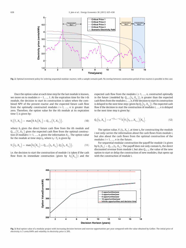
Fig. 2. Optimal investment policy for ordering sequential modular reactors, with a sample scenario path. No overlap between construction period of two reactors is possible in this case.

628 S. Jain et al. / Energy Economics 36 (2013) 625–636

Once the option value at each time step for the lastmodule is known,we move on to modules n−1, …, 1. At the expiration time for the i-thmodule, the decision to start its construction is taken when the com-bined NPV of the present reactor and the expected future cash flowfrom the optimally constructed modules i+1, …, n is greater thanzero. Therefore, the option value for the ith module at its expirationtime Ti is given by:

Vi Ti;XTi

� �¼ max 0;hi XTi

� �þ Qiþ1 Ti;XTi

� �� �; ð10Þ

where hi gives the direct future cash flow from the ith module andQiþ1 Ti;XTi

� �gives the expected cash flow from the optimal construc-

tion of modules i+1, …, n, given the information XTi. The option value

for the module at time step tk, where tkbTi, is given by

Vi tk;Xtk

� �¼ max hi Xtk

� �þ Qiþ1 tk;Xtk

� �;Qi tk;Xtk

� �� �; ð11Þ

i.e. the decision to start the construction of module i is taken if the cashflow from its immediate construction (given by hi Xtk

� �) and the

2 4 6 8200

250

300

350

400

450

Decision H

Op

tio

n V

alu

e(E

uro

s/kW

)

Fig. 3. Real option value of a modular project with increasing decision horizon and exerciseelectricity is 3 cents/kWh and volatility in electricity price is 20%.

expected cash flow from the modules i+1, …, n, constructed optimallyin the future (modeled by Qiþ1 tk;Xtk

� �), is greater than the expected

cashflows from themodules i,…,n, if the decision to start its constructionis delayed to the next time step (given byQi tk;Xtk

� �). The expected cash

flow if the decision to start the construction of modules i,…, n is delayedto the next time step is given by:

Qi tk;Xtk

� �¼ e−r tkþ1−tkð ÞE Vi tkþ1;Xtkþ1

� �Xtk

��� i:

hð12Þ

The option value, Vi tk;Xtk

� , at time tk for constructing the module

i not only carries the information about the cash flows frommodule i,but also about the cash flows from the optimal construction of themodules i+1, …, n in the future.

For sequential modular construction the payoff for module i is givenby hi Xtk

� þ Qiþ1 tk;Xtk

� . The payoff does not only contain hi, the direct

discounted revenue from module i, but also Qi+1, the value of the newoption to start or delay the construction of newmodules, that opens upwith the construction of module i.

10 12 14 16 18

orizon (years)

2 opportunities/year4 opportunities/year8 opportunities/year16 opportunities/yearInfinite opportunities and decision time

opportunities per year compared with the value obtained by Gollier. The initial price of

2 4 6 8 10 12 14 162

2.5

3

3.5

4

4.5

Time (years)

Ele

ctri

cty

Pri

ce (

cen

ts\k

Wh

)

Critical Price 1st Module ( Finite Horizon)Critical Price 1st Module (Perpetual Option)

Fig. 4. Critical price at which the first module should be ordered, comparison between finite time and infinite time horizon.

629S. Jain et al. / Energy Economics 36 (2013) 625–636

4. Stochastic grid method for multiple exercise options

The real option problems we are interested in, have financial coun-terparts, i.e. the Bermudan options andmultiple exercise Bermudan op-tions. A Bermudan option gives the holder the right, but not obligation,to exercise the option once, on a discretely spaced set of exercise dates.Amultiple exercise Bermudanoption, on the other hand, can be exercisedmultiple times before the option expires. Pricing of Bermudanoptions, es-pecially for multi-dimensional processes is a challenging problem owingto its path-dependent settings.

Consider an economy in discrete time defined up to a finite timehorizon Tn. The market is defined by the filtered probability spaceΩ;F ;F t ;Pð Þ. Let Xt, with t=t0, t1, ots, tm=Tn, be an Rd-valued discretetimeMarkov chain describing the state of the economy, the price of theunderlying assets and any other variables that affect the dynamics ofthe underlying. HereP is the risk neutral probabilitymeasure. The hold-er of the multiple exercise Bermudan option has n exercise opportuni-ties, that can be exercised at t0, t1, …, tm. Let hi(Xt) represent thepayoff from the ith exercise of the option at time t and underlyingstate Xt. The time horizon for the ith exercise opportunity is given by Ti.

We define a policy, π, as a set of stopping times τn, …, τ1 withτnb…bτ1, which takes values in t0, …, tm=Tn, and τi determines the

0 2 4 6 8150

200

250

300

350

400

Decision H

Op

tio

n V

alu

e (E

uro

s/kW

)

Fig. 5. Real option value for the large reactor and the modular project for diffe

timewhere the ith remaining exercise opportunity can be used. The op-tion value when there are n early exercise opportunities remaining isthen found by solving an optimization problem, i.e. to find the optimalexercise policy, π, for which the expected payoff is maximized. Thiscan be written as:

Vn t0;Xt0¼ x

� �¼ sup

πEXnk¼0

hk Xτk

� �jXt0

¼ x

" #: ð13Þ

In simple terms, Eq. (13) states that of all possible policies for or-dering the reactor in the given decision horizon, the real option valueis computed using the one which maximizes the expected future cashflows.

In the past decade several simulation-based algorithms have beenproposed for pricing Bermudan options. The regression based approachproposed by Carriere (1996), Tsitsiklis and Van Roy (1999) was popu-larized as the least squares method (LSM) by Longstaff and Schwartz(2001). Other important approaches include the stochastic meshmeth-od of Broadie and Glasserman (2004), computing the early exercisefrontier by Ibanez and Zapatero (2004) and the duality based methodfrom Haugh and Kogan (2004) and Rogers (2002). More recently Jain

10 12 14 16 18

orizon (years)

Large ReactorModular Case

rent decision horizons when the initial price of electricity is 3 cents/kWh.

1 9 17−1

−0.5

0

0.5

1

1.5

2x 105

Decision Horizon (years)

Exp

ecte

d C

ash

Flo

w (

Eu

ros)

1st Module2nd Module3rd Module4th Module

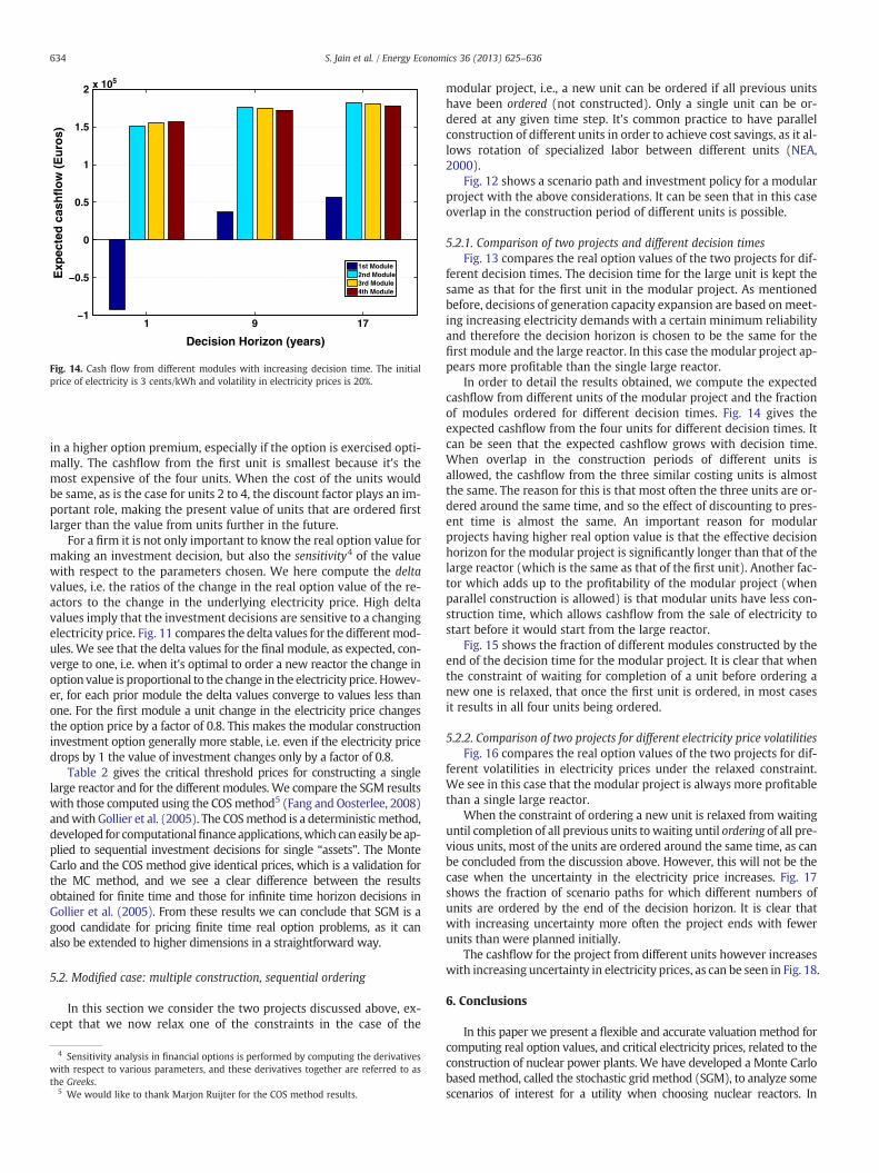
Fig. 6. Cash flow from different modules with increasing decision time. The initial priceof electricity is 3 cents/kWh and the volatility in electricity prices is 20%.

630 S. Jain et al. / Energy Economics 36 (2013) 625–636

and Oosterlee (2012) proposed the stochastic grid method (SGM) forpricing high-dimensional Bermudan options.

The problem of pricing Bermudan options with multiple exercise op-portunities has been dealt with by Meinshausen and Hambly (2004),with generalizations by Bender (2009), Aleksandrov and Hambly(2008) and Schoenmakers (2012), who use the dual representation forsuch pricing problems. Chiara et al. (2007) apply the multiple exercisereal options in infrastructure projects. They use a multi-least-squaresMonte Carlo method for determining the option value.

The problem of sequential modular construction stated above canbe solved using the stochastic grid method (Jain and Oosterlee, 2012).We choose the stochastic grid method, because:

• The stochastic grid method (SGM) can efficiently solve the multipleexercise Bermudan option problem;

• SGM can be used to compute the sensitivities of the real option value;• The method can be easily extended to higher dimensions;• The method doesn't depend on the choice of the underlying stochas-tic process;

• Improved confidence intervals are obtained with fewer paths whencompared to LSM.

Although the problemwe consider here is one-dimensional, with theelectricity price as the stochastic variable, a typical real option problem

10

5

10

15

20

25

30

35

40

45

Decision Ho

% P

ath

s

Fig. 7. Fraction of modules ordered in the end for different scenario paths with increasing deprices is 20%.

tends to be high-dimensional with several underlying stochastic terms.A proper choice of pricing method would be one which can be extendedto higher dimensions in the future.

The stochastic grid method solves a general optimal stopping timeproblem using a hybrid of dynamic programming and Monte Carlosimulation. The method first determines the optimal stopping policyand a direct estimator for the option price. The optimal stopping pol-icy for the ith module at time step tk involves finding the critical elec-tricity price X�

tk. When the market price of electricity is equal to the

critical price, the value of delaying the construction of the moduleto the next time step is equal to the value of starting the constructionimmediately, i.e.,

Qi tk;X�tk

� �¼ hi X�

tk

� �:

Therefore, the critical price is taken to be the largest grid point Xtk ,for which Qi tk;Xtk

� > hi Xtk

� . The module is ordered if the present

market price of electricity is greater than the critical price for thegiven time step. Once the policy for all the time steps is known, SGMcomputes lower bound values, using a new set of simulated electricitypaths, as the mean of the cashflows from each simulated path wherethe module is ordered following the policy obtained above.

SGM for multiple exercise Bermudan options begins by generatingN stochastic paths for the electricity prices, starting from initial stateX0. The electricity prices realized by these paths at time step tk consti-tute the grid points at tk. The electricity price paths can be generatedusing Eq. (5) here.

The pricing steps for SGM can be decomposed into two main parts,based on the recursive dynamic programming algorithm from the pre-vious section.

• Parametrization of the option value: The option values at each gridpoint are converted into a functional approximation using piece-wiseregression.

• Computation of the continuation value: The continuation value is com-puted using the conditional probability density function and the func-tional approximation of the option value at the next time step.

4.1. Parametrization of the option value

In order to obtain the continuation value for grid points at tk, we needto determine the functional approximations of the option value at tk+1.Once the option values at the grid points at tk+1are known, the functionalapproximation is obtained using a piece-wise least squares regression.Therefore, the option value at a given time step is divided into two re-gions, separated by the critical electricity price X�

tkþ1.

7 17

rizon (years)

No Module

Only 1st Module

1st and 2nd Module

1st, 2nd and 3rd Module

All 4 Modules

cision time. The initial price of electricity is 3 cents/kWh and the volatility in electricity

15 20 25 30 35250

300

350

400

450

500

550

600

650

Electriicty Price Volatility (%)

Op

tio

n V

alu

e (E

uro

s/kW

) Modular ReactorLarge Reactor

Fig. 8. Real option value for the large reactor and the modular project for different volatilities when the decision horizon is 9 years and the initial price of electricity is 3 cents/kWh.

631S. Jain et al. / Energy Economics 36 (2013) 625–636

For the two segments the functional approximation is given by,

V̂ i tkþ1;Xtkþ1

� �¼ 1

Xtkþ1bX�

tkþ1

n oXM−1

m¼0

amXmtkþ1

þ 1Xtkþ1

≥X�tkþ1

n oXM−1

m¼0

bmXmtkþ1

: ð14Þ

The expression 1Xtkþ1bX�

tkþ1

n o is an indicator function whose

value equals 1, if the argument Xtkþ1bX�tkþ1

n o, is true and it is 0 other-

wise. Therefore, 1Xtkþ1bX�

tkþ1

n o and 1Xtkþ1≥X�

tkþ1

n o group the grid

points into two segments, separated by the critical electricity price.The results converge to the true price when increasing number ofsegments are used (see Jain and Oosterlee, 2012).

4.2. Computation of the continuation value

Once the functional approximations of the option values for mod-ules i and (i+1) are known for time step tk+1, the continuation valuefor the ith module at tk can be computed using Eq. (12). In order tocompute the expectation, E Vi tkþ1;Xtkþ1

� Xtk

�� �, we need the distribu-

tion function for Xtkþ1 given Xtk . This conditional distribution function,f Xtkþ1 Xtk ¼ x

�� �, for the GBM process is known in closed form.

10% 20

10

20

30

40

50

60

Elec Pric

Per

cen

tag

e P

ath

s

Fig. 9. Fraction of modules ordered in the end for different scenario paths with increasing vfirst module is 9 years.

Therefore, the continuation value, or the value of the reactor if the de-cision to order it is delayed to the next time step, as given Eq. (12) canbe written as:

Q̂ i tk;Xtk

� �¼ ∫y∈ 0;X�½ �

XM−1

m¼0

amym

!f yð jXtk

¼ xÞdy

þ ∫y∈ X� ;∞ð �XM−1

m¼0

bmym

!f yð jXtk

¼ x

Þdy: ð15Þ

In a more generic case where the conditional distribution functionis unknown, it can be approximated using the Gram Charlier Series.For more details on computing the continuation value, we refer to(Jain and Oosterlee, 2012).

5. Numerical experiments

We consider the case where an investor needs to decide betweentwo projects, one involving a single large reactor of 1200 MWe andthe other consisting of four modules of 300 MWe each. The construc-tion time and costs for the two projects, given in Table 1, are takenfrom the reference case by Gollier et al. (2005). The discount rate istaken as 8% per annum, which is the OECD average, and the predictedgrowth rate of electricity price is 0% here. The cost of electricity pro-duction for the first unit is relatively expensive when compared to se-ries units, as a large part of the fixed costs for the modular assembly,

0% 30%

e Volatility

No ModulesOnly 1st Module1st and 2nd Module1st, 2nd and 3rd ModuleAll 4 Modules

olatility. The initial price of electricity is 3 cents/kWh and the decision horizon for the

3 3.25 3.5 3.75 4 4.25 4.5 4.750.4

0.5

0.6

0.7

0.8

0.9

1

1.1

Electricity Price (cents/kWh)

Del

ta

1st Module2nd Module3rd Module4th Module

Fig. 11. The delta values for the four modules when the decision horizon is 12 yearsand the volatility in electricity price is 20%.

632 S. Jain et al. / Energy Economics 36 (2013) 625–636

like the land rights, access by road and railway, site licensing cost, areconnection to the electricity grid are carried by the first unit.

In the case of the modular project we consider two different con-straints, in two subsections to follow, i.e., the decision for construc-tion of subsequent units can be made:

1. Once the construction of all prior units is completed (similar to thecase considered by Gollier),

2. Once the decision for the construction of all prior units has beentaken. Also, only one unit can be ordered at a given time step.

5.1. Sequential construction: the case in Gollier et al. (2005)

In this test case we apply constraint 1 for the construction of sub-sequent modules, i.e., the decision for the construction of a new mod-ule will not be made, unless the construction of all previous modulesis finalized. By the SGM we first obtain an optimal investment policyand a direct estimator of the real option value of the project. The op-timal policy gives the critical electricity price (as a function of time),above which a module should be ordered. At a given time a newmod-ule is ordered only when the present electricity is higher than the cor-responding critical price for the module under consideration andwhen all other constraints are satisfied. Once the optimal investmentpolicy is obtained, a fresh set of electricity paths is generated, and ateach of these simulated paths a new module is decided if the follow-ing conditions are satisfied:

1. All modules preceding the given module have been constructed.2. The present electricity price is higher than critical price for order-

ing the given module.3. The present time is within the decision horizon for the corre-

sponding module.4. The given module hasn't been ordered so far for the given path.

Fig. 2 illustrates for a sample electricity path when a new moduleshould be ordered. A module is ordered once the above conditions aresatisfied and the revenue from this module is discounted back to theinitial time. The mean of the discounted revenue for different pathsfrom all the four modules gives the real option value of the project.For a single large reactor the steps followed are the same, exceptthat condition 1 is not required.

As the case in Gollier et al. (2005) corresponds to an infinite hori-zon decision problem with exercise opportunities, we compare itwith an increasing finite time decision horizon. Fig. 3 compares the

10 20 30−0.5

0

0.5

1

1.5

2

2.5 x 105

Volatility (%)

Exp

ecte

d C

ash

flo

w (

Eu

ros)

1st Module2nd Module3rd Module4th Module

Fig. 10. Expected cashflow from different units for different volatility values for elec-tricity prices. The initial price of electricity is 3 cents/kWh and the decision horizonfor the first module is 9 years.

real option value of the modular project with the reference value inGollier et al. (2005). The option value of the project doesn't increasemuch with an increasing number of exercise opportunities per year,however it increases significantly with an increasing decision hori-zon. From Fig. 3 it's clear that the real option value of a modular pro-ject with a realistic decision horizon is lower than the value obtainedin Gollier et al. (2005), where an infinite decision horizon is assumed.In other simulations, not reported here, we found that the optionvalue of the modular project with the same parameters, but with adecision horizon of 100 and 200 years and four exercise opportunitiesper year, has an option value between 390 and 400 Euro/kW, which isalready closer to the infinite horizon values.

Fig. 4 then compares the optimal investment policy for the firstmodule with the corresponding policy in Gollier et al. (2005). Itshows clearly the effect of a finite decision horizon on the investmentpolicy. As one approaches the final decision time, the value of waiting(given by the continuation value) reduces which lowers the thresholdelectricity price at which a new module should be ordered. However,in the case of an infinite decision time horizon, the optimal policy orthreshold electricity price remains constant with time.

5.1.1. Comparison of two projects with different decision timesWe now compare the real option values of the two projects, i.e. the

single large reactor and the sequence of small modular units, for increas-ing decision time horizon and uncertainty in electricity prices. The con-struction costs and times for the reactors are taken from Table 1. Basedon Eq. (6), we take the corresponding decision horizon for the construc-tion of the first module between 1 and 17 years. For the single large re-actor we take the decision horizon the same as that for first module.One of the advantages of a modular construction is that the increasingdemand can be met gradually, which allows the spreading of the deci-sions to a longer time horizon, possibly without significant gaps in

Table 2Critical threshold electricity prices (cents/KWh) at which new reactors should be or-dered, for different decision horizons. There are twenty equally spaced exercise oppor-tunities each year. The volatility of the electricity price is taken as 20%.

Final decision Isolated Modular

Time (years) LR Unit 1 Unit 1 Unit2 Unit3 Unit 4

SGM 12 4.56 5.98 4.05 3.44 3.65 3.9317 4.60 6.02 4.18 3.50 3.69 3.9622 4.62 6.05 4.24 3.53 3.71 3.98

COS 12 4.56 5.98 4.10 3.46 3.65 3.9317 4.60 6.03 4.21 3.51 3.69 3.9622 4.62 6.05 4.25 3.53 3.71 3.98

Gollier ∞ 4.75 6.23 4.29 3.57 3.79 4.10

0 2 4 6 8 10 12 14 161.5

2

2.5

3

3.5

4

4.5

5

5.5

6

Time (years)

Ele

ctri

city

Pri

ce (

cen

ts/k

Wh

)

Critical Price for 1Critical Price for 2Critical Price for 3Critical Price for 4Scenario Electricity Path

ConstructionMod 2

Construction Mod 1

ConstructionMod 3

Fig. 12. Optimal investment policy for ordering sequential modular reactors, with a sample scenario path. Overlap between construction period of two reactors is possible in thiscase.

633S. Jain et al. / Energy Economics 36 (2013) 625–636

demand and supply. Therefore, although the decision horizon for thefirst module can be small, the decision horizon for the entire projectcan be longer.

Fig. 5 compares the option value for the single large reactor withthat for the modular project for increasing decision time. When thedecision horizon is small it is optimal to opt for the large reactorwhereas for longer decision horizons modular projects appear moreprofitable.

An insight into the reason why modular projects are better for lon-ger decision time is given by Fig. 6, which shows the expected cashflowfrom the four units for increasing decision time. When the decision ho-rizon is small, the expected cashflow from the first module can be neg-ative, which is the casewhen the decision horizon for thefirstmodule is1 year. For short decision times, the first unit needs to be ordered tokeep open the option to order more profitable subsequent modules.As the time approaches the final decision time for the first unit, it canbe ordered even if the expected revenue from its construction wouldbe negative.With increasing decision horizon the investor canwait lon-ger and order the modules at more profitable electricity prices.

Fig. 7 shows fractions of the scenario paths forwhich different num-bers of modules are ordered. When the decision horizon is small, theproject is only partially completed for a large number of scenariopaths, making it unprofitable. However, for longer decision times, thefraction of the scenario paths for which all the four modules are

0 2 4 6 8150

200

250

300

350

400

450

500

Decision H

Op

tio

n V

alu

e (E

uro

s/kW

)

Fig. 13. Real option value for the large reactor and the modular project for diffe

constructed increases, while the fraction of partially completed projectreduces.

5.1.2. Comparison of two projects and different volatilities in electricityprices

A parameter to be considered when deciding between a singlelarge reactor and the modular project is the uncertainty in electricityprices. We compare the real option value of the two projects for in-creasing volatility in the electricity price in Fig. 8.

When the volatility in the electricity price is low, the single largereactor project is more profitable, while for higher volatilities themodular project seems a better choice. An intuitive answer to this isthat, for high volatilities, modular projects offer more flexibility, i.e.,if the electricity price path at some point reaches unfavorable prices,the possibility to abandon module construction, with a few units al-ready ordered, exists. Fig. 9 shows the fraction of scenario paths forwhich the modular project finishes with different numbers of unitsordered. As expected, the fraction of paths for which not all the fourunits are ordered increases with increasing volatility.

Fig. 10 gives the expected cashflow from each unit for differentvolatilities of the electricity prices. In general, the option value ofthe project increases with an increasing uncertainty. A higher volatil-ity reflects greater future price fluctuations (in either direction) inunderlying electricity price levels. This expectation generally results

10 12 14 16 18

orizon (years)

Modular CaseLarge Reactor

rent decision horizons when the initial price of electricity is 3 cents/kWh.

1 9 17−1

−0.5

0

0.5

1

1.5

2 x 105

Decision Horizon (years)

Exp

ecte

d c

ash

flo

w (

Eu

ros)

1st Module2nd Module3rd Module4th Module

Fig. 14. Cash flow from different modules with increasing decision time. The initialprice of electricity is 3 cents/kWh and volatility in electricity prices is 20%.

634 S. Jain et al. / Energy Economics 36 (2013) 625–636

in a higher option premium, especially if the option is exercised opti-mally. The cashflow from the first unit is smallest because it's themost expensive of the four units. When the cost of the units wouldbe same, as is the case for units 2 to 4, the discount factor plays an im-portant role, making the present value of units that are ordered firstlarger than the value from units further in the future.

For a firm it is not only important to know the real option value formaking an investment decision, but also the sensitivity4 of the valuewith respect to the parameters chosen. We here compute the deltavalues, i.e. the ratios of the change in the real option value of the re-actors to the change in the underlying electricity price. High deltavalues imply that the investment decisions are sensitive to a changingelectricity price. Fig. 11 compares the delta values for the differentmod-ules. We see that the delta values for the final module, as expected, con-verge to one, i.e. when it's optimal to order a new reactor the change inoption value is proportional to the change in the electricity price. Howev-er, for each prior module the delta values converge to values less thanone. For the first module a unit change in the electricity price changesthe option price by a factor of 0.8. This makes the modular constructioninvestment option generally more stable, i.e. even if the electricity pricedrops by 1 the value of investment changes only by a factor of 0.8.

Table 2 gives the critical threshold prices for constructing a singlelarge reactor and for the different modules. We compare the SGM resultswith those computed using the COSmethod5 (Fang and Oosterlee, 2008)andwith Gollier et al. (2005). The COSmethod is a deterministic method,developed for computationalfinance applications,which can easily be ap-plied to sequential investment decisions for single “assets”. The MonteCarlo and the COS method give identical prices, which is a validation forthe MC method, and we see a clear difference between the resultsobtained for finite time and those for infinite time horizon decisions inGollier et al. (2005). From these results we can conclude that SGM is agood candidate for pricing finite time real option problems, as it canalso be extended to higher dimensions in a straightforward way.

5.2. Modified case: multiple construction, sequential ordering

In this section we consider the two projects discussed above, ex-cept that we now relax one of the constraints in the case of the

4 Sensitivity analysis in financial options is performed by computing the derivativeswith respect to various parameters, and these derivatives together are referred to asthe Greeks.

5 We would like to thank Marjon Ruijter for the COS method results.

modular project, i.e., a new unit can be ordered if all previous unitshave been ordered (not constructed). Only a single unit can be or-dered at any given time step. It's common practice to have parallelconstruction of different units in order to achieve cost savings, as it al-lows rotation of specialized labor between different units (NEA,2000).

Fig. 12 shows a scenario path and investment policy for a modularproject with the above considerations. It can be seen that in this caseoverlap in the construction period of different units is possible.

5.2.1. Comparison of two projects and different decision timesFig. 13 compares the real option values of the two projects for dif-

ferent decision times. The decision time for the large unit is kept thesame as that for the first unit in the modular project. As mentionedbefore, decisions of generation capacity expansion are based onmeet-ing increasing electricity demands with a certain minimum reliabilityand therefore the decision horizon is chosen to be the same for thefirst module and the large reactor. In this case the modular project ap-pears more profitable than the single large reactor.

In order to detail the results obtained, we compute the expectedcashflow from different units of the modular project and the fractionof modules ordered for different decision times. Fig. 14 gives theexpected cashflow from the four units for different decision times. Itcan be seen that the expected cashflow grows with decision time.When overlap in the construction periods of different units isallowed, the cashflow from the three similar costing units is almostthe same. The reason for this is that most often the three units are or-dered around the same time, and so the effect of discounting to pres-ent time is almost the same. An important reason for modularprojects having higher real option value is that the effective decisionhorizon for the modular project is significantly longer than that of thelarge reactor (which is the same as that of the first unit). Another fac-tor which adds up to the profitability of the modular project (whenparallel construction is allowed) is that modular units have less con-struction time, which allows cashflow from the sale of electricity tostart before it would start from the large reactor.

Fig. 15 shows the fraction of different modules constructed by theend of the decision time for the modular project. It is clear that whenthe constraint of waiting for completion of a unit before ordering anew one is relaxed, that once the first unit is ordered, in most casesit results in all four units being ordered.

5.2.2. Comparison of two projects for different electricity price volatilitiesFig. 16 compares the real option values of the two projects for dif-

ferent volatilities in electricity prices under the relaxed constraint.We see in this case that the modular project is always more profitablethan a single large reactor.

When the constraint of ordering a new unit is relaxed from waitinguntil completion of all previous units to waiting until ordering of all pre-vious units, most of the units are ordered around the same time, as canbe concluded from the discussion above. However, this will not be thecase when the uncertainty in the electricity price increases. Fig. 17shows the fraction of scenario paths for which different numbers ofunits are ordered by the end of the decision horizon. It is clear thatwith increasing uncertainty more often the project ends with fewerunits than were planned initially.

The cashflow for the project from different units however increaseswith increasing uncertainty in electricity prices, as can be seen in Fig. 18.

6. Conclusions

In this paper we present a flexible and accurate valuation method forcomputing real option values, and critical electricity prices, related to theconstruction of nuclear power plants. We have developed a Monte Carlobasedmethod, called the stochastic grid method (SGM), to analyze somescenarios of interest for a utility when choosing nuclear reactors. In

15 20 25 30 35200

300

400

500

600

700

800

Volatility in Elec Prices (%)

Op

tio

n V

alu

e (E

uro

s/kW

h)

Modular ProjectLarge Reactor

Fig. 16. Real option value for the large reactor and the modular project for different volatilities when the decision horizon is 9 years and the initial price of electricity is 3 cents/kWh.

1 9 170

10

20

30

40

50

60

Decision Horizon (years)

Per

cen

tag

e P

ath

s

No ModulesOnly 1st Module1st and 2nd Module1st, 2nd and 3rd ModuleAll 4 Modules

Fig. 15. Fraction of modules ordered at the end for different scenario paths with increasing decision times. The initial price of electricity is 3 cents/kWh and the volatility in elec-tricity prices is 20%.

635S. Jain et al. / Energy Economics 36 (2013) 625–636

particular, we have focused our attention to the modular constructionand finite decision horizons.

Some of the outcomes can be summarized as:

• SGM is a suitable Monte Carlo method for pricing real options, es-pecially for valuing projects with modularity. The method has

10% 20

10

20

30

40

50

60

70

Elec Pric

Per

cen

tag

e P

ath

s

Fig. 17. Fraction of modules ordered at the end for different scenario paths with increasingfirst module is 9 years.

been validated against the deterministic COS method for a 1D testcase.

• Most investment decision problems are governed by a finitedecision time. It has been shown, in various numerical experi-ments, that decision-making in finite time may result in quite dif-ferent scenarios compared to infinite time decision problems.

0% 30%

e Volatility

No ModulesOnly 1st Module1st and 2nd Module1st, 2nd and 3rd ModuleAll 4 Modules

volatility. The initial price of electricity is 3 cents/kWh and the decision horizon for the

10 20 30−0.5

0

0.5

1

1.5

2

2.5 x 105

Volatility(%)

Exp

ecte

d C

ash

flo

ws

(Eu

ros)

1st Module2nd Module3rd Module4th Module

Fig. 18. Expected cashflow from different units for different volatilities of electricityprices. The initial price of electricity is 3 cents/kWh and the decision horizon for thefirst module is 9 years.

636 S. Jain et al. / Energy Economics 36 (2013) 625–636

• When the modular project has a restriction on parallel construc-tion of different units then:– The real option value of a single large reactor is typically higher

when decision horizons are small.– For longer decision timesmodular projectsmay bemore profitable.– With an increasing uncertainty in the electricity prices, modeled

by a higher volatility in the chosen electricity price model, modularconstruction may represent a better option. Modular constructionmay include the possibility of having a few units ordered, whenthe electricity price reaches unfavorable values. With stable elec-tricity prices the cost effective single large reactor appears to be abetter choice.

• When there is the possibility of parallel construction ofmodular units,then:– the option value of the modular project greatly improves, and

seems, with our model assumptions, more profitable than a sin-gle large reactor for different decision horizons.

– For different electricity price volatility values, the modular pro-ject seems to be the better choice.

– In many cases, once the first unit of the modular project is or-dered it results in all units being ordered.– The option value of the modular project greatly improves, and

seems, with our model assumptions, more profitable than asingle large reactor for different decision horizons.

– For different electricity price volatility values, the modular pro-ject seems to be the better choice.

– In many cases, once the first unit of the modular project is or-dered it results in all units being ordered.

This paper serves as a validation of our method against the resultsobtained in Gollier et al. (2005). In our future research, a more de-tailed analysis may include a sophisticated electricity price model, de-mand and capacity factors, and stochastic construction and operationcosts. In a follow-up paper we also discuss the impact of features likethe construction of twin reactors (parallel construction of modules),effect of learning and rare events on the real option values of variousscenarios.

It's worth noting that the real option values computed here does notinclude electricity price predictionmodel uncertainty, which is typicallycalled model risk in finance. We presume here that the electricity price

follows GBM and the scenario paths used for calculations follow thesame model. In reality however, the model presumed by a firmwouldn't exactly replicate the actual electricity price process distribu-tion.Model risk can however be assessed by varying the price dynamicsand studying the impact on the real option values. Furthermore, one canalways compute sensitivities with respect to the different problem pa-rameters. In the present paper however, the purpose of the study wasto compare two projects in which case the electricity price predictionmodel uncertainty effects the valuation of both of them similarly.

References

Aleksandrov, N., Hambly, B.M., 2008. A dual approach to multiple exercise option problemsunder constraints. Math. Meth. Oper. Res. 71 (3), 503–533.

Arrow, K.J., Fischer, A.C., 1974. Environmental preservation, uncertainty and irrevers-ibility. Q. J. Econ. 88, 312–319.

Barlow, M., 2002. A diffusion model for electricity prices. Math. Finance 12 (4),287–298.

Bender, C., 2009. Dual pricing of multi exercise options under volume constraints. Fi-nance Stoch. 15 (1), 1–26.

Boarin, S., Locatelli, G., Mancini, M., Ricotti, E., 2012. Financial case studies on small andmodular reactors. Nucl. Technol. 178.

Brennan, M.J., Schwartz, E.S., 1985. Evaluating natural resource investments. J. Bus. 58,135–157.

Broadie, M., Glasserman, P., 2004. A stochastic meshmethod for pricing high-dimensionalAmerican option. J. Comput. Finance 7, 35–72.

Carelli, M.D., Garrone, P., Locatelli, G., Mancini, M., Mycoff, C., Trucco, P., Ricotti, M.E.,2010. Economic features of integral, modular, small-to-medium size reactors.Prog. Nucl. Energy 52, 403–414.

Carriere, J.F., 1996. Valuation of the early exercise price for derivative securities usingsimulation and splines. Insurance: Mathematics and Economics 19, 19–30.

Chiara, N., Garvin, M.J., Vecer, J., 2007. Valuing simple multiple-exercise real options ininfrastructure projects. J. Infrastruct. Syst. 13 (2), 97–104.

Dixit, A.K., Pindyck, R.S., 1994. Investment Under Uncertainty. Princeton UniversityPress, Princeton.

Fang, F., Oosterlee, C.W., 2008. A novel pricing method for European options based onFourier-cosine series expansions. SIAM J. Sci. Comput. 31, 826–848.

Gollier, C., Proult, D., Thais, F., Walgenwitz, G., 2005. Choice of nuclear power investmentsunder price uncertainty: valuing modularity. Energy Econ. 27, 667–685.

Haugh, M., Kogan, L., 2004. Approximating pricing and exercising of high-dimensionalAmerican options: a duality approach. Oper. Res. 52 (2), 258–270.

Henry, C., 1974. Investment decisions under uncertainty: the irreversibility effect. Am.Econ. Rev. 64, 1006–1012.

Ibanez, A., Zapatero, F., 2004. Monte Carlo valuation of American options through com-putation of the optimal exercise frontier. J. Financ. Quant. Anal. 39 (2), 253–275.

Jain, S., Oosterlee, C.W., 2012. Pricing high-dimensional Bermudan options using thestochastic grid method. Int. J. Comput. Math. 89 (9), 1186–1211.

Kessides, I.N., 2010. Nuclear power: understanding the economic risks and uncer-tainties. Energy Policy 38, 3849–3864.

Longstaff, F.A., Schwartz, E.S., 2001. Valuing American options by simulation: a simpleleast-squares approach. Rev. Financ. Stud. 3, 113–147.

Lucia, J.J., Schwartz, E.S., 2002. Electricity prices and power derivatives: evidence fromthe Nordic power exchange. Rev. Deriv. Res. 5 (1), 5–50.

McDonald, R., Siegel, D., 1986. The value of waiting to invest. Q. J. Econ. 101, 707–727.Meinshausen, N., Hambly, B.M., 2004. Monte Carlo methods for the valuation of multi-

exercise options. Math. Finance 14 (4), 557–583.NEA, 2000. Reduction of Capital Costs of Nuclear Power Plants. OECD/NEA.Paddock, J.L., Siegel, D.R., Smith, J.L., 1988. Option valuation of claims on real assets: The

case of offshore petroleum leases. The Quarterly Journal of Economics 103 (3),479–508.

Pilipovic, D., 1998. Energy Risk: Valuing and Managing Energy Derivatives. McGrawHillPublishers.

Pindyck, R.S., 1993. Investments of uncertain costs. J. Financ. Econ. 34, 53–76.Rogers, L.C.G., 2002. Monte Carlo valuation of American options. Math. Finance 12,

271–286.Rothwell, G., 2006. A real options approach to evaluating new nuclear plants. Energy J.

27 (1), 37–53.Schoenmakers, J., 2012. A pure martingale dual for multiple stopping. Finance and Sto-

chastics 16 (2), 319–334.Trigeorgis, L., 1996. Real Options: Managerial Flexibility and Strategy in Resource Allo-

cation. MIT Press, Cambridge, MA.Tsitsiklis, J., Van Roy, B., 1999. Optimal stopping of Markov processes: Hilbert space

theory, approximation algorithms, and an application to pricing high-dimensionalfinancial derivatives. IEEE Transactions on Automatic Control 44, 1840–1851.