Valuing electricity-dependent infrastructure:

An essential-input approach

Jed Cohen1, Klaus Moeltner2, Johannes Reichl3, and Michael Schmidthaler4

1Department of Agricultural and Applied Economics, Virginia Tech, jedcohen@vt.edu2Department of Agricultural and Applied Economics, Virginia Tech, moeltner@vt.edu∗

3The Energy Institute at Johannes Kepler University, Linz, Austria, reichl@energieinstitut-linz.at4The Energy Institute at Johannes Kepler University, Linz, Austria,

schmidthaler@energieinstitut-linz.at

August 18, 2016

Abstract

Electricity is an essential input to both the production of household commodities,and the provision of public infrastructure services. The latter, in turn, are essential tothe generation of additional household goods. Thus, customers’ willingness to pay toavoid power interruptions will reflect both aspects of foregone household production.We recognize this as an opportunity to value infrastructure services via stated preferencemethods based on power outage scenarios. We develop a hybrid model that combineshousehold production theory with a Random Utility framework to derive Europeanhouseholds’ willingness-to-pay to avoid disruption of electricity provision to the “frontdoor,” as well as the loss of important public services. We find that a considerableportion of total willingness-to-pay, to the order of 20-80%, relates to the public servicecomponent. This stresses the importance of explicitly specifying the scale of outagesand their effect on public services in stated preference elicitation. Failure to do so willproduce welfare estimates that are unfit to inform policy, and normalized outage costestimates that are biased - potentially by a very large margin.

keywords: Power outages, public infrastructure, multivariate probit, Bayesian estimation

1 Introduction

Climate change poses increasing risks to the reliable provision of electricity around the

globe. On the supply side, increasing temperatures and more frequent heat waves decrease

the efficiency of thermal and nuclear power plants by hampering thermal conversion, and

∗Corresponding author: 208 Hutcheson Hall, Blacksburg, VA 24061; phone: (540) 231-8249. This researchproject was supported under the program “Regional Competitiveness Initiative Upper Austria 2007-2013,”by the provincial government of Upper Austria (contract # 225865). Funding for all survey work wasprovided through the research project SESAME (EU Framework 7 Programme, contract # 261696).

1

by reducing the availability and ability of water for cooling. Hydropower plants, in turn,

are vulnerable to extreme precipitation and flood events, as well as inter-annual variation

in inflows (Arent et al., 2014). All types of supply installations in low-lying areas are at an

increased risk of flooding (Davis and Clemmer, 2014). On the transmission and distribution

side, more frequent violent storms damage transmission lines and other elements of the

electric grid year-round. Wildfires, which are increasing in frequency and ferocity, directly

destroy electric infrastructure, and interfere with the conductivity of transmission lines

(Davis and Clemmer, 2014). On the demand side, rising temperatures and intense heat

waves increase the demand for cooling in many regions, further taxing the capacity of the

electricity system (Davis and Clemmer, 2014). All these risks lead to more frequent and

prolonged power interruptions. For the example, in the U.S. the average annual number of

weather-related power outages has doubled between 2003 and 2012, affecting an average of

15 million customers each year (Kenward and Raja, 2013).

Climate change also affects other elements of the public infrastructure, such as water

supply, sanitation services, and transportation. Water supply is affected both in terms

of quantity due to reduced renewable surface and groundwater resources in many regions,

and in terms of quality due to increased sedimentation and runoffs, as well as disruption

of treatment facilities during floods (IPCC, 2014). More frequent heavy rainfall events

can also overload the capacity of sewer systems and wastewater treatment plants, causing

disruptions in sanitation services (Arent et al., 2014). Transportation services, in turn, are

vulnerable to flooding, will require higher maintenance due to larger temperature swings,

and face cooling challenges in many parts of the world (Arent et al., 2014). Naturally,

disruptions in any of these primary services can, in turn, affect the provision of health and

emergency services (IPCC, 2014).

Importantly for our study, all of these public services rely to a large extent on the

provision of electricity. Therefore, climate change is expected to exacerbate disruptions

of basic infrastructure services directly, via the factors mentioned above, and indirectly,

by increasing the risk of power outages. In consequence, the economic value of electric

service reliability is intrinsically linked to the societal value of other segments of the public

2

infrastructure. Our analysis exploits this linkage to elicit values for both power provision

and power-dependent infrastructure services (ISs).

Overall, this study contributes to the valuation literature along three dimensions. First,

we add to the outage cost literature by dis-aggregating total willingness-to-pay (WTP) to

avoid a power interruption into values lost due to electricity not delivered directly to the

household (i.e. the “front door”), and values lost due to interrupted ISs in the house-

holds’ neighborhood or region. This informs decisions regarding the optimal provision of

these services, which are often largely funded by taxpayers, as well as the prioritization of

infrastructure protection from power interruptions.

Second, we add estimates to the sparse literature that has attempted to value public or

semi-public ISs in the developed world. We argue that using an essential input approach

to generate these estimates may be less controversial in a stated preferences (SP) setting

than proposing a hypothetical scenario of a complete loss or severe degradation of these

taken-for-granted services due to institutional or policy reasons.

Third, at a theoretical level, we show how the concept of an “essential input” and

a household production framework, both traditionally employed in a revealed preferences

(RP) context, can be fruitfully combined with SP elicitation to learn about consumer wel-

fare associated with public and semi-public services. Specifically, we illustrate how typical

Random Utility Models (RUMs) used for power outage cost estimation flow naturally from

the conceptual starting point of a household production framework, with electricity taking

the role of the essential input.

We find that a sizable portion of average hourly outage costs, to the order of 20-80%,

can be attributed to lost ISs for our sample of residents from eight European countries.

Customers are especially sensitive to losing medical, communication, transportation, and

sanitation services. Our findings raise serious concerns about using the common “WTP /

kilowatt hour (kwh) unserved” metric to express outage impacts to residents, since kwh

unserved are traditionally computed at the “front door,” whereas, as shown in this study,

household WTP relates to a much broader set of impacts and thus a much larger volume

of lost electric load.

3

1.1 Power outages and infrastructure services

It is well documented that large-scale power outages can severely affect critical elements

of the public infrastructure. For example, as summarized by Public Safety and Emergency

Preparedness Canada (2006), the Northeastern Interconnection power outage of 2003, at-

tributed to an overloaded grid, affected 50 million people in the U.S. and Canada, and

impacted “virtually all ten critical infrastructure sectors,” such as banking services, food

distribution, waste water treatment, traffic lights, highway signs, gas pumps, and even

internet services and firewalls, which exposed customers to multiple cyber threats.

A 2003 storm-related outage that affected most of Italy brought trains to a standstill

and disrupted communication and telephone services (BBC News, 2003). An overload in

Germany’s power network triggered widespread outages in five European countries in late

fall of 2006, leaving people stuck in elevators and delaying numerous trains (BBC News,

2006). A 2007 winter storm that hit the U.S. Midwest caused large-scale outages that left

people without electric heat or lights, halted airport operations, and disrupted water supply

to thousands of residents due to the failure of electric pumps (NBC News, 2007). In 2012, a

series of thunder storms caused power outages affecting nearly four million customers in the

mid-Atlantic and South-Eastern region of the U.S., cutting out traffic lights, halting train

services, and even knocking out Amazon’s cloud (data storage) services, with the cascading

effect of interrupting popular internet sites and services such as Netflix and Instagram (CNN

News, 2012).

It is therefore well conceivable that respondents have these IS interruptions in mind

when asked to think about their WTP to avoid a specific outage scenario. However, with the

exception of Reichl et al. (2013), none of the published outage cost studies based on survey

methods elaborate on the spatial scale of a stipulated interruption.1 Households are either

told that, for additional payments, front-door delivery of power will remain uninterrupted

(Layton and Moeltner, 2005; Carlsson and Martinsson, 2007), or asked to choose from a set

of outage bundles that vary in timing, length and / or frequency, and are each linked to a

1Using a repeated discrete choice format similar to that employed in this study, Reichl et al. (2013)stipulate outages that differ in scale between “street-only” and “province-level” to their sample of Austrianhouseholds. However, they do not report scale-specific WTP estimates.

4

specific fee added to the electricity bill (Beenstock et al., 1998; Carlsson and Martinsson,

2008; Baarsma and Hop, 2009; Blass et al., 2010).

In the first case, elicited WTP can only be interpreted as values for household commodi-

ties produced exclusively with front-door electricity (refrigeration, meals, hair drying, etc.)

and provides no guidance as to the broader societal value of protecting or maintaining ISs.

The second approach raises even bigger issues, as it is not clear which outage scale, and

thus the extent of impact on ISs, respondents have in mind when they select from a given

outage choice menu. This makes it impossible to clearly assign derived WTP estimates to

front-door losses versus ISs-related damages, and, in turn, makes it difficult to use resulting

estimates for policy purposes.

1.2 Valuing infrastructure services

The ISs considered in this study are best described as semi-public goods, as they are all

associated with fees, and are - at least to some extent - provided by commercial entities.

However, most of them are typically subsidized by the government (medical care, water and

sanitation services, public transit) or require publicly financed infrastructure (gas pipelines,

road maintenance, traffic lights and signage, land and access roads for cell phone towers,

etc.). In addition, some of them are overseen by public utility commissions that have

considerable control over service scope, quality, and pricing (e.g water and sanitation).

Thus, to the extent that taxpayer moneys are involved in the provision and maintenance

of these services, it is economically meaningful to think of an optimal level of provision. This,

in turn, requires information on costs and benefits. In many cases, the latter will be difficult

to gauge based on observed behavior alone, given muddled price signals due to subsidies,

regulation, or lack of temporal or spatial variability. As in many other such cases, this

suggests elicitation approaches based on SP methods.

We are aware of only a handful of studies that have attempted to value essential pub-

lic services in developed countries. For example, Hensher et al. (2005) and Willis et al.

(2005) use a Contingent Experiment (CE) approach to estimate households’ WTP for un-

interrupted water and sanitation services in Australia and England, respectively. Hackl

5

and Pruckner (2006), using contingent valuation (CV) methods, elicit Austrian households’

values for publicly funded emergency medical services, using a scenario of “possible future

privatization.” Schwarzlose et al. (2014) implement a CE in three Texan counties to elicit

stakeholders’ values of various public transportation attributes, with focus on expanded

services for the elderly and using private car registration fees as payment vehicle. Savage

and Waldman (2009), also employing a CE, estimate customers’ WTP for various attributes

of home internet service, such as reliability, speed, and independence of phone connections.

While all these studies find that people care about these services, such direct SP ap-

proaches also carry with them a set of empirical risks. As discussed in Hensher et al. (2005)

and Willis et al. (2005), given the critical nature of some of these services to cover basic

human needs, and a lack of historic problems with service provision, respondents may ques-

tion the realism of stipulated interruption scenarios. Furthermore, any suggestions of taking

away services traditionally provided by local governments will undoubtedly trigger protest

responses, and may introduce sample selection problems into the empirical analysis.

However, as discussed above and as is evident from our empirical data, most house-

holds, even in developed countries, will have experienced power outages in recent history.

Furthermore, large scale outages are highly publicized in the media, reaching a population

well beyond actually affected residents. Therefore, the notion of losing ISs that are reliant

on electric power should not appear foreign and inconceivable to survey respondents. This

should mitigate any realism problems that may arise with more direct cessation-of-service

scenarios. In our application, we have a second built-in safeguard against a lack of buy-in

for stipulated scenarios. Specifically, as described below in more detail, we let respondents

decide themselves if they believe specific ISs will be affected in their neighborhood or region

by a prolonged outage. We find pronounced WTP premia for households that hold such

beliefs.

1.3 Household production and essential inputs

As discussed in detail in upper-level textbooks (e.g. Bockstael and McConnell, 2007; Phaneuf

and Requate, forthcoming), the household production approach to the valuation of some

6

quasi-fixed public good, say q, rests on the notion that both q and observed market goods x

enter a household technology function that combines these inputs to generate useful services,

say H. Importantly, aside from its contribution to the provision of these services, q does not

otherwise enter the consumer’s utility function. In this situation, the researcher has several

options to empirically derive utility-theoretic welfare estimates for small changes in q that

hold utility and household production fixed - using data on either production technology,

production costs, or the input demand for x.

Furthermore, Bockstael and McConnell (1983) show that utility-theoretic welfare mea-

sures for larger changes in q can be obtained in the special case where x is an essential input

in the production of H. That is, if x is zero, no H can be produced, regardless of the level of

q. This then allows the analyst to directly relate welfare effects due to a change in q to the

difference in the areas under the Hicksian demand curves for the private input x, evaluated

at the initial and changed level of q. Standard methods can then be employed to approx-

imate this measure using observed Marshallian demand for x (Bockstael and McConnell,

1993; Smith and Banzhaf, 2004; von Haefen, 2007).

In this study, electricity is the essential input for household production of electricity-

dependent goods and services, while elements of the public infrastructure (water and sani-

tation, public transportation, communication and internet, etc.) take the role of the (semi-)

public good q. Using a household production framework and exploiting electricity’s essential

good - property, we show that welfare measures related to the the provision of electricity

can be unambiguously interpreted as values for electricity-dependent household production.

Furthermore, using a survey-based identification strategy, we show that a good portion of

these values can be attributed to lost ISs. Conceptually, the only difference between our

framework and a traditional household production approach is that we use SP methods to

estimate electricity-related welfare estimates rather than RP methods based on observed

demand. As such, our methodology could be interpreted as a novel hybrid RP-SP approach,

at least at a conceptual level.

7

2 Modeling Framework

2.1 Conceptual model

A given household depends on electricity provision in two ways to produce household goods

and services, such as warm meals, ironed shirts, online shopping, and entertainment: (i) It

uses electricity directly delivered to the “front door,” and (ii) it uses semi-public ISs such

as the internet, ATM machines, and cell phone communication that themselves depend on

electricity.

Let H1 be a vector of k1 household-produced, infrastructure-independent goods, each

of which uses electricity e1k (e.g. operating a stove), household labor l1k (e.g. cooking a

meal), and other market inputs x1k (e.g. groceries). The production technology for the

entire bundle can then be expressed as

H1 = f1 (e1, l1,x1) , (1)

where vectors e1, l1, and x1 comprise the inputs for the k1 services.

Analogously, let H2 be a vector of k2 household-produced, infrastructure-dependent

services, each of which uses elements of the public infrastructure Gk (e.g. internet service),

household labor l2k (e.g. time spent on the computer), and other market inputs x2k (e.g.

PC, high-speed modem, etc.). The production technology for the entire bundle can then be

expressed as

H2 = f2 (G (e2,g) , l2,x2) , (2)

where the vector notation is as before. Importantly, as denoted in equation (2), the infras-

tructure services depend themselves on electricity e2, in addition to other inputs g that are

exogenous to the household. Moreover, electricity is an essential input for the production of

H1, and - via its pivotal role in the provision of G, also the production of H2. We therefore

8

have the essential input restrictions

H1| (e1 = 0) = f1 (0, l1,x1) = 0, and

H2| (e2 = 0) = f2 (G (0,g) , l2,x2) = f2 (0, l2,x2) = 0

(3)

Given our focus on power outages that last for a relatively short time horizon, we will

treat the household’s market inputs related to the use of infrastructure services (x2), which

will primarily be durable goods such as communication or computing devices, as fixed in

the following derivation.

Following standard reasoning for household production models (e.g. Bockstael and Mc-

Connell, 2007; Phaneuf and Requate, forthcoming) the household’s optimization problem

can be conceptually described as a two-step process: First, the household chooses home-

used electricity e1, market inputs x1, labor allocations l1 and l2, and public services G to

achieve a certain level of household services H1 and H2 at the lowest possible cost. This

produces the cost function

C (pe,p1,pG,H1,H2) = mine1,x1,l1,l2,G

{pee1 + p′1x1 + p′GG (.) +

λ′1 (H1 − f1 (.)) + λ′2 (H2 − f2 (.)) + λ3

(L−

k1∑k=1

l1k −k2∑k=1

l2k

)},

(4)

where pe is the price of electricity, and p1 and pG are, respectively, the price vectors for x1

and G, L is the total available amount of at-home labor, and the λ terms are multipliers.

This cost function then feeds into the second conceptual step, in which the household

maximizes utility over H1, H2, and a numeraire commodity z, subject to constraints for

9

budget, technology, and labor, that is:2

maxe1,x1,l1,l2,G,z

U (H1,H2, z) s.t.

m = C (pe,p1,pG,H1,H2) + z

H1 = f1 (e1, l1,x1)

H2 = f2 (G (e2,g) , l2,x2)

L =

k1∑k=1

l1k +

k2∑k=1

l2k

(5)

where m is the total available household budget. Assuming interior solutions for all choice

variables, this yields the indirect utility function

U (H∗1,H∗2, z∗) , with

H∗1 = f1 (pe,p1,pG,m,L)

H∗2 = f2 (pe,p1,pG,m,L) and

z∗ = z (pe,p1,pG,m,L)

(6)

where we continue to implicitly condition on x2. In a standard household production

framework the next step would be to invoke the essential input condition and express com-

pensating variation (CV) for a change in G (potentially down to zero) as the area between

two shifted Hicksian demands for e2, and use observed demand for e2 to approximate this

amount. In our case, this is problematic since electricity e2 needed to run G is beyond the

control of an individual household, so there are no choke prices or observed demands for

this input at the household level.

Instead, we now switch to a stated preference framework to estimate welfare associated

with lost ISs, asking respondents to choose between payment to avoid a specific (widespread)

outage, or tolerate the interruption at no loss of income. We exploit the essential input

condition in the sense that if the interruption takes place, all of e1, e2, G, H1, and H2

2In the interest of parsimony but without loss in generality we abstract from any labor-leisure decisionsin our model.

10

are driven to zero. Therefore, the estimated WTP to avoid the outage can be directly

interpreted as the welfare losses associated with foregone production and consumption of

household goods and services. Furthermore, since G is itself an essential input in the

production of H2, as is evident from the second line in (3), welfare losses associated with

ceased production of H2 can be unambiguously interpreted as the CV for the availability of

G. As mentioned above, we use a survey-based identification strategy to extract this latter

component of WTP.

Approximating indirect utility in (6) with a standard linear form and adding a random

error term allows us to cast the household problem in a Random Utility Modeling (RUM)

framework. Specifically, let indirect utility for household i under uninterrupted electricity

service during a specific time frame s (e.g.: summer weekday, 6 am - 10 am) be given as

U∗si = ds{H∗1i

′β∗1s + H∗2i′β∗2s

}+ τmi − ds

{τ(pee∗1i + p′1x

∗1i + p′GG∗i (.)

)}+ εsi (7)

where ds measures the number of time periods (hours), the β∗ and τ terms are model coef-

ficients, εsi is a time-sensitive, idiosyncratic error term, and we have used the relationship

z∗i = mi − ds (pee∗1i + p′1x

∗1i + p′GG∗i ).

Now consider a blackout during the exact same time frame. This implies that neither

home-used electricity e1 nor any of the semi-public services G will be available, driving the

home production of H1 and H2 to zero. At the same time, the household will not incur

any expenses for electricity e1 and public infrastructure G. However, a perishable share of

private inputs, say αx1i, with 0 ≤ α ≤ 1, will be lost in case of an outage.

The indirect utility function thus reduces to

U∗s,i0 = τmi − dsταp′1x∗i1 + εs,i0 (8)

where we specify a different idiosyncratic error εs,i0 to accommodate additional or different

unobservables that may enter indirect utility in case of a power outage compared to the

case of power provision.

The compensating variation (willingness-to-pay) CVsi to avoid this outage scenario “s”

11

is then implicitly defined as

U∗si (mi − CVsi) = U∗s,i0, (9)

which, using (7) and (8) yields

CVsi = ds{H∗1i

′β1s + H∗2i′β2s

}− ds

{pee∗1i + (1− α) p′1x

∗i1 + p′GG∗i (.)

}+ εsi

where βrs =β∗rsτ, r = 1, 2 and εsi =

εsi − εs,i0τ

(10)

As is clear from this derivation CVsi includes components related to both infrastructure-

independent and infrastructure-dependent household services. It represents the lost value

of both types of home production, minus foregone expenditures from not using electricity

or public infrastructure services, and the value of non-perishable inputs that can be used

at a later point in time.

If the household is offered bid Psi to avoid an outage of type s, it will take the contract

if its willingness to pay exceeds the bid, that is if

Usi = CVsi − Psi =

ds{H∗1i

′β1s + H∗2i′β2s

}− ds

{pee∗1i + (1− α) p′1x

∗i1 + p′GG∗i (.)

}− Psi + εsi > 0

(11)

where Usi is the economic surplus left to the household after paying to avoid the outage.

Adding a statistical distribution for the error term produces the increasingly popular “sur-

plus” version of the random utility model, aka “estimation in willingness-to-pay (WTP)

space” (e.g. Train and Weeks, 2005; Sonnier et al., 2007; Scarpa et al., 2008).

Empirically, this conceptual framework can be made operational by letting

Usi = ds(h′iβhs + r′siβrs

)− Psi + εsi, (12)

where hi is a vector of household characteristics, rsi is a vector of binary indicators for

infrastructure services, and the β terms are corresponding coefficients. Specifically, in our

empirical application the elements rsi take on a value of one if household i believes the

corresponding infrastructure service will be affected by outage scenario s, and a value of

12

zero otherwise.

The interaction h′iβhs captures the net value of lost infrastructure-independent produc-

tion per hour of interruption, that is the term H∗1i′β1s− pee∗1i− (1− α) p′1x

∗i1 in (11). This

leaves r′siβrs to measure the net value of lost household production per hour of outage that

is dependent on infrastructure services, i.e. the term H∗2i′β2s − p′GG∗i (.) in (11).

2.2 Econometric model

Our survey elicits households’ WTP a specified bid Psi to avoid outage scenario s, for a set

of S different interruptions, each distinguished by duration, time of occurrence, and season,

as described in more detail in the next section. Allowing for unrestricted error correlations,

the full system of S surplus equations can thus be written as

U1i = d1

(h′iβh1 + r′1iβr1

)− P1i + ε1i

U2i = d2

(h′iβh2 + r′2iβr2

)− P2i + ε2i

...

USi = dS(h′iβhS + r′SiβrS

)− PSi + εSi, with

εi =

[ε1i ε2i . . . εSi

]′∼ n (0,Σ) and

Σ =

σ211 σ12 . . . σ1S

σ21 σ222 . . . σ2S

......

. . ....

σS1 σS2 . . . σ2SS

,

(13)

where σkl = σlk ∀ l 6= k. Thus, our combined error vector follows a multivariate normal

distribution with zero mean and a full variance-covariance matrix. It should be noted that

despite the binary nature of the observed dependent variables (yes/no responses) all terms

in Σ are identified, since responses are given with respect to a known numerical threshold

(the stipulated bid). Furthermore, we allow all surplus variances to be scenario-specific.

Since our stipulated outages differ in duration this allows ex ante for more uncertainty from

13

unobservables (i.e. a larger error variance) for longer interruptions. This is confirmed in

our empirical application.

Individual i’s contribution to the likelihood function is the joint probability of observing

the S-fold vector of outage responses yi. Expressing latent WTP (that is surplus Usi minus

bid Psi) as y∗si and collecting all S bids offered to respondent i in Pi, and all IS-responses

in ri this term can be written as:

prob (yi|hi, ri,Pi;β,Σ) = prob

b1i,l < y∗1i < b1i,u

b2i,l < y∗2i < b2i,u...

bSi,l < y∗Si < bSi,u

=

Φi (hi, ri,Pi;β,Σ;Ti) ,

(14)

where β =

[β′1 β′2 . . . β′S

]′, and bsi,l and bsi,u designate, respectively, the lower and

upper threshold for latent WTP, as implied by the observed response ysi. Specifically,

bsi,l = Psi and bsi,u =∞ if ysi = 1 (“yes”). If a negative response is observed, i.e. ysi = 0,

we have bsi,l = −∞ and bsi,u = Psi. As indicated by the last line of (14) this joint probability

can be concisely expressed as an S-fold cumulative normal density Φi, truncated to the S-

dimensional region Ti.

For the sample at large the likelihood function is thus given by

prob (y|H,R,P;β,Σ) =

N∏i=1

Φi (.) , (15)

where vector y comprises all individuals’ outage responses and P collects all individual bid

vectors. Analogously, matrices H and R collect all hi and ri, respectively.

Maximum likelihood estimation of this model would be cumbersome for this high-

dimensional equation system with individual-specific truncation restrictions. We therefore

opt for a Bayesian estimation framework. The resulting Gibbs Sampler (GS) is straightfor-

ward to implement and converges after a reasonable number of burn-ins. The GS draws con-

14

secutively and repeatedly from the conditional posterior distributions p(β| {y∗i }

Ni=1 ,H,R,P; Σ

),

p(Σ| {y∗i }

Ni=1 ,H,R,P;β

)and p

({y∗i }

Ni=1 |y,H,R,P;β,Σ

), where vector y∗i combines la-

tent WTP for all S outage equations for household i. Posterior inference is based on the

marginals of the joint posterior distribution p (β,Σ|y,H,R,P). Further details for this GS

and its implementation are given in a separate online appendix.

2.3 Posterior predictions of WTP

Collecting primary parameters β and Σ in vector θ, the GS yields draws of θ from the joint

posterior distribution p (θ|y,H,R,P). Posterior predictive distributions (PPDs) of the

expected hourly WTP for the typical household in each country, for each of the four outage

scenarios, can be obtained in straightforward manner. For each draw of βs from the GS we

compute wtpsc|βs = 1nc

∑i∈c (h′iβhs + r′siβrs), that is the sample average of observation-

specific estimates of expected hourly WTP for country c. Repeating this computation for all

draws of βs from the original sampler yields the desired PPD, which can then be examined

for its statistical properties.

As discussed below in more detail, setting all elements of βrs to one (zero) produces

WTP predictions for an otherwise typical household that believes that all (none) of the

public services are affected.

3 Empirical Application

3.1 Data

Our data are based on survey of residential electricity customers conducted between fall

2012 and spring 2013 in all 27 EU nations at that time. The survey team contacted over

176,000 households and recruited between 260 and 300 respondents in each member state,

taking efforts to assure representativeness for the respective underlying population along

key demographic dimensions, such as geographic location, gender and age of the head of

household, employment status, and income. Households had the choice to complete the

questionnaire by phone or online. Details of the sampling process and survey implementa-

15

tion are given in Garcia Gutierrez et al. (2013), appendices A-D.3

Importantly, a few weeks prior to the actual telephone or online survey, each participant

was sent a confirmation letter that reminded them “to be conscious of their surroundings

and activities and think about all the ways they use electricity in their daily life,” to get

them to start thinking of the potentially widespread effects of a power outage.

Three parts of the questionnaire are relevant for this study. Part one collected back-

ground information on respondents’ experience with power outages. In addition, households

were asked to indicate on an ordinal scale to what extent they believed each of eight es-

sential ISs would be affected by a prolonged outage. Part two elicited their WTP to avoid

each of a set of eight unplanned power interruptions. Part three then collected standard

information on household demographics.

For this study we focus on four of the stipulated interruptions that were described as

occurring at the country-level, as opposed to being highly localized (“street level”). This

assures that respondents could reasonably assume that ISs were affected by such widespread

events.

Furthermore, we narrow our sample to a subset of eight countries that share a similar

outage history and, on average, hold similar beliefs regarding affected ISs. This choice

is largely driven by data limitations given our modest sample sizes at the country level.

Specifically, preliminary analyses indicated clearly that the marginal effects of covariates

differ significantly across outage scenarios, i.e. coefficient vectors βhs and βrs in (12) are

truly scenario specific, as presumed in our conceptual notation in the previous section.

This preempts any pooling of parameters across outages. The resulting large parameter

space (close to 90 estimable model coefficients, plus six variance-covariance terms) does not

leave enough degrees of freedom to estimate country-specific models with any reasonable

3Given budget constraints, the survey team aimed for an initial target of 250 participating households percountry. This level was exceeded in all cases. Households were initially contacted by telephone or e-mail andasked about their willingness to participate in a subsequent telephone or online survey. This first contactalso served as a screening tool to eliminate households that did not fit within the demographic target quotas.The recruiting/screening procedure was carried out until about 125-150 participants per country agreed toparticipate in a phone interview and 100-125 agreed to participate in the online survey. Those who did fitthe target quotas and agreed to participate were sent a confirmation letter that contained the survey bookletor a web link to the booklet. A second phone call was then made to walk the respondent through the survey.Online participants were sent a survey link instead.

16

degree of precision. We therefore opt to pool our data across a sub-set of countries that are

homogeneous in key aspects of this study, especially in beliefs regarding IS interruptions.

To determine such homogeneity, we computed the percentage of households that believed

that a given IS would be affected for each country and IS. We then examined the deviations

of these shares across all eight ISs and all 27 countries. The final set of eight nations

exhibits a deviation in average shares over all ISs of no larger than 8%, and a deviation

in IS-specific shares of 20% or less across all public services. In conjunction with similar

income levels in most of these countries and a comparable degree of (high) historic power

reliability, we take this as an indication that citizens of these nations are also likely to share

similar preferences for infrastructure services. We thus pool these data and estimate a single

set of coefficients per outage scenario for all eight nations. This strikes us as a reasonable

compromise between allowing marginal effects - and thus average hourly WTP - to remain

scenario-specific, while preserving a full set of explanatory variables and a large enough

sample size to assure identification.

The resulting set of countries, listed in alphabetical order and comprising a total of

1807 households, is given in Table 1. As is evident from the first column, most of these

nations have been EU members for at least 40 years, with Austria and Sweden (1995)

constituting more recent additions. Sample sizes, after dropping observations with missing

key information, are comparable across countries (column two), and so are measures of

historic outage frequency (columns five through seven), and satisfaction levels with the local

utility (last column). The survey also elicited information on the longest outage respondents

had experienced in the preceding five-year period. As can be seen from columns eight and

nine, the resulting implicit distribution of maximum outage length differs somewhat across

countries, with Belgium and Luxembourg exhibiting the largest share of relatively short

“longest outages” (< 1 hour), and Sweden and the UK showing the highest percentage of

respondents that experienced an outage exceeding four hours in duration.

The eight nations also differ markedly in annual per capita electricity consumption

(column three), with Sweden (4100 kwh) taking the lead and the Netherlands showing up

as the thriftiest member (1496 kwh). The Danish pay by far the highest price for electricity

17

(e0.30/kwh, column four), while the remaining countries face similar prices, in the e0.17-

0.23 range.4

Table 1: Power provision statistics by country (2012)

year sample annual price/ longest outage satisfiedjoined size kwh/ kwh num. of out. last yr. last 5 yrs. w. utility

country EU (HHs) p.c. (euros) % zero mean std. < 1 hour > 4hrs (%)

Austria 1995 230 2093 0.20 48.3% 1.4 1.9 18.3% 13.0% 100%Belgium 1958 214 1789 0.23 55.1% 1.4 2.9 20.1% 10.7% 94%Denmark 1973 213 1790 0.30 59.2% 1.1 1.9 16.4% 11.7% 98%Ireland 1973 235 1772 0.22 61.7% 0.9 1.5 6.0% 17.0% 97%

Luxembourg 1958 206 1746 0.17 57.8% 0.9 1.6 26.7% 8.3% 99%Netherlands 1958 230 1496 0.19 61.7% 0.8 1.4 15.2% 16.5% 97%

Sweden 1995 234 4100 0.20 60.3% 1.2 2.4 17.1% 21.8% 96%UK 1973 245 1807 0.17 56.3% 1.2 2.0 9.8% 19.2% 98%

kwh = kilowatt hour / std. = standard deviation / p.c. = per capita / num. = number / yr. = year

Table 2 shows aggregate respondent and household characteristics for our sample. Over-

all, our data display a good representation of female respondents (41-53%), a comparable

age structure across countries, and expected average household sizes in the range of 2-3

persons. The degree of urbanization (column 4) differs markedly across nations, from less

than 50% in Austria to close to 80% in Denmark. The majority of respondents in each

country hold an A-level diploma (a requirement for university entry), with Ireland and the

Netherlands falling slightly below the 50% mark. Households in Luxembourg have the high-

est average income (close to e50,000/year), while the other nations show similar averages

in the mid-e20,000’s to low e30,000s range.5

The survey template with the IS perception questions is given in appendix A. Each

table row corresponds to one of eight essential services: medical care (including emergency

response, henceforth abbreviated as “medical”), fuel and gas supply (for private and public

transportation, as well as heating, “fuel/gas”), electronic payment options (ATM use, credit

card transactions, electronic banking, “payments”), communication (land and mobile tele-

4Statistics on electrity consumptions in 2012 were obtained from European Commission (2016a). Elec-tricity prices for 2012 are given in European Commission (2016b).

5Income was computed based on the midpoints of ten interval bins. We approximate the upper bound ofthe highest category as the lower bound of that category plus the bandwidth of the preceding bin. Householddemographics for all 27 EU nations are given in Cohen et al. (2016).

18

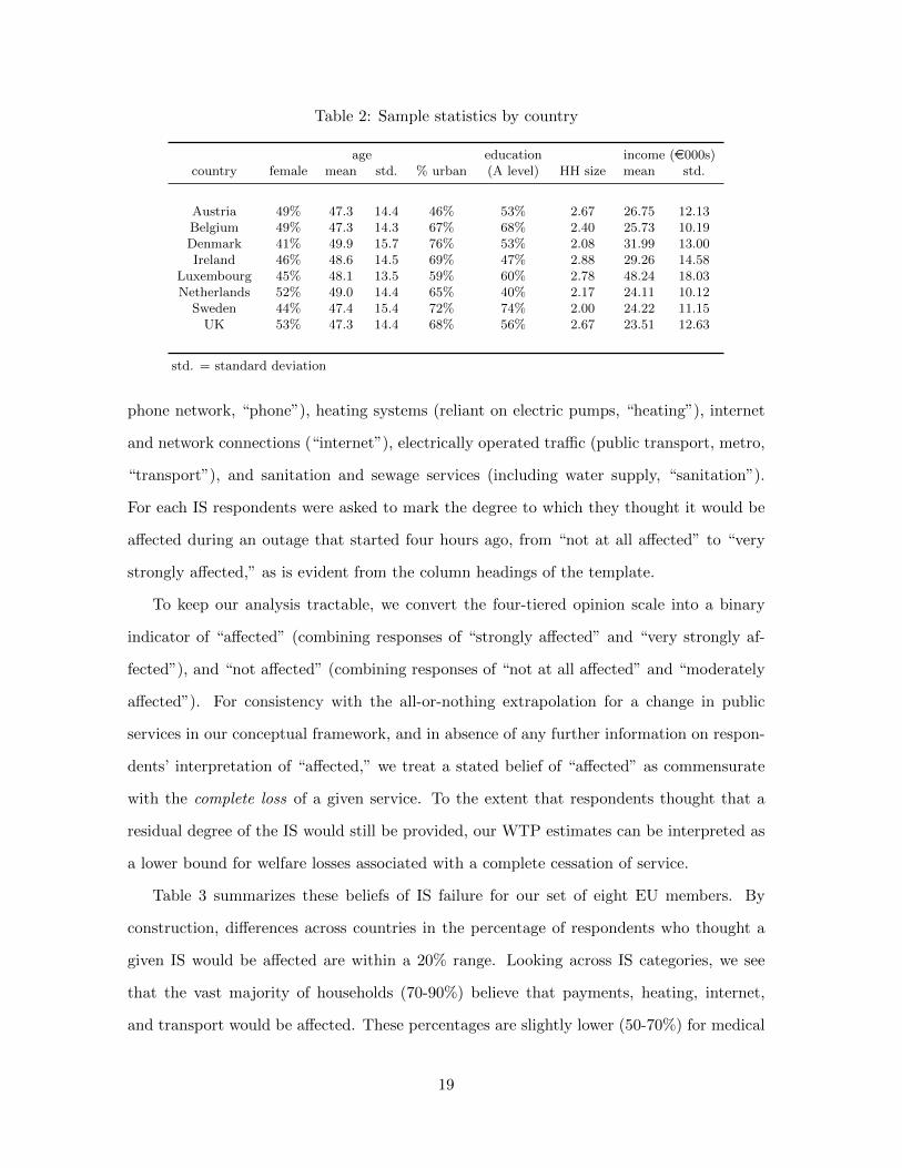
Table 2: Sample statistics by country

age education income (e000s)country female mean std. % urban (A level) HH size mean std.

Austria 49% 47.3 14.4 46% 53% 2.67 26.75 12.13Belgium 49% 47.3 14.3 67% 68% 2.40 25.73 10.19Denmark 41% 49.9 15.7 76% 53% 2.08 31.99 13.00Ireland 46% 48.6 14.5 69% 47% 2.88 29.26 14.58

Luxembourg 45% 48.1 13.5 59% 60% 2.78 48.24 18.03Netherlands 52% 49.0 14.4 65% 40% 2.17 24.11 10.12

Sweden 44% 47.4 15.4 72% 74% 2.00 24.22 11.15UK 53% 47.3 14.4 68% 56% 2.67 23.51 12.63

std. = standard deviation

phone network, “phone”), heating systems (reliant on electric pumps, “heating”), internet

and network connections (“internet”), electrically operated traffic (public transport, metro,

“transport”), and sanitation and sewage services (including water supply, “sanitation”).

For each IS respondents were asked to mark the degree to which they thought it would be

affected during an outage that started four hours ago, from “not at all affected” to “very

strongly affected,” as is evident from the column headings of the template.

To keep our analysis tractable, we convert the four-tiered opinion scale into a binary

indicator of “affected” (combining responses of “strongly affected” and “very strongly af-

fected”), and “not affected” (combining responses of “not at all affected” and “moderately

affected”). For consistency with the all-or-nothing extrapolation for a change in public

services in our conceptual framework, and in absence of any further information on respon-

dents’ interpretation of “affected,” we treat a stated belief of “affected” as commensurate

with the complete loss of a given service. To the extent that respondents thought that a

residual degree of the IS would still be provided, our WTP estimates can be interpreted as

a lower bound for welfare losses associated with a complete cessation of service.

Table 3 summarizes these beliefs of IS failure for our set of eight EU members. By

construction, differences across countries in the percentage of respondents who thought a

given IS would be affected are within a 20% range. Looking across IS categories, we see

that the vast majority of households (70-90%) believe that payments, heating, internet,

and transport would be affected. These percentages are slightly lower (50-70%) for medical

19

fuel/gas, and phone, while only 40-50% of respondents worry about impacted sanitation

services. Overall, therefore, our data exhibits sufficient variability in beliefs to identify an

IS effect, that is to dis-entangle total WTP to avoid a given outage into WTP to preserve

household production related to front-door electric service, and WTP to avoid a loss of

services related to the public infrastructure.

Table 3: Infrastructure failure perceptions by country (%)

medical fuel/gas payments phone heating internet transport sanitation

Austria 55 57 79 69 74 82 89 50Belgium 55 50 70 63 71 72 82 45Denmark 60 53 81 62 73 79 88 57Ireland 60 56 77 54 80 82 83 40

Luxembourg 55 59 69 66 79 76 75 50Netherlands 63 55 77 73 74 67 85 50

Sweden 56 48 80 59 64 79 85 55UK 72 57 77 62 77 78 85 46

Entries show the percentage of respondents that believed that a given infrastructure service would bestrongly or very strongly affected after four hours of power interruption.

Each country-level outage scenario presented to the respondents is unplanned, and de-

fined by duration (1, 4, 12, 24 hours), and season (summer, winter). Respondents were given

the option to pay a specified bid (in form of an add-on to their next electricity bill) and

avoid the outage or to decline payment and experience the interruption. Importantly, we

stressed that the extra payment would leave the household completely unaffected, including

“all important services discussed in the last section.”6

Our preference elicitation format thus corresponds to a repeated, single-bounded discrete-

choice format as employed in Layton and Moeltner (2005), Carlsson and Martinsson (2007),

and Reichl et al. (2013). The settings for duration generally reflect the spectrum found in

the existing literature (e.g. Layton and Moeltner, 2005; Carlsson and Martinsson, 2007,

2008; Baarsma and Hop, 2009; Reichl et al., 2013). All of our stipulated outages occur on

6To provide some technical realism linking payment to protection, respondents were told that “Thesedays there are technical solutions that can prevent critical events from leading to power outages, such asweather-resistant underground cables and smarter switchgear equipment. These measures improve servicereliability significantly, especially during critical events, but their cost is also significant.” This was followedby the actual elicitation question: “For each scenario ... I will read out a sum of money and ask you to tellme whether you think you would prefer to pay this sum and therefore not be affected by this power outage,or whether you would prefer not to pay but instead experience this outage.”

20

a weekday and include a time span of likely high activity in the household, i.e. either early

morning or early evening.

Table 4 depicts the outage attributes for the four country-level scenarios. Figure 1 shows

an example of an outage scenario, as it was presented to the respondent.

Table 4: Attribute settings for outage scenarios

scenario duration season time span(hours)

1 1 winter 8pm-9pm2 4 summer 6am-10am3 12 summer 8am-8pm4 24 winter 10am-10am

Figure 1: Outage scenario example

We stipulated between three and four country-specific bid values per outage scenario.7

The bid design was informed by a recent study on energy reliability in Austria (Reichl et al.,

2013). Specifically, we adopt the four bids administered in that survey for outages of equal

length to those in our scenarios, with an adjustment for income differences between Austria

and the other seven countries in our set.8 During sampling, the survey team examined the

share of “yes” responses for all bids and countries for the first 25 observations to assure

adequate coverage. This screening process did not prompt any ex-post adjustments to the

7Originally, a total set of four bids were selected for each country across all eight outage scenarios. Sincewe only consider the national-scale interruptions for this analysis, the number of effective bids is reducedto three for some country / scenario combinations, and - in the case of Luxembourg - to two for the firstscenario.

8The bids in the Austrian study were derived based on a D-optimality criterion with balanced utilities(Huber and Zwerina, 1996; Burgess and Street, 2003, 2005; Ferrini and Scarpa, 2007).

21

bid ladders. The full set of bid amounts and share of “yes” responses for each scenario

and country are given in Table 6 in appendix B. As is evident from the table, with few

exceptions the percentage of “yes” responses decreases monotonically over increasing bids,

as expected.

3.2 Estimation results

We implement our correlated binary choice model with fixed effects for each country to

capture unobserved differences in relevant aspects of power provision. Household vector hi

in (13) includes three age categories (35-45 years, 46-60 years, over 60 years, with omitted

baseline of 20-35 years), an indicator for an “urban” residential location (as opposed to

suburban or rural), an indicator for gender (with “female” the omitted baseline), household

size, and educational attainment (an indicator equal to one if the respondent holds an A-level

diploma). Household characteristics also include the historic 12-month outage frequency,

indicator categories for the longest outage experienced in the preceding five years (1-4 hours,

4-8 hours, 8-24 hours, and over 24 hours, with < 1 hour the implicit baseline category), and

a binary indicator variable for the household’s declared satisfaction with the local power

utility (1 = “very” or “fairly” satisfied, 0 = “not very” or “not at all” satisfied).

This is followed by the eight IS indicators (vector rsi in (13)), each taking value of one

if a given respondent believed the service in question would be affected, and a value of zero

otherwise. As discussed above, the marginal effects for all variables in hi and rsi are allowed

to vary over the four scenarios.

Our specification is completed by a binary indicator “scenario ordering,” taking a value

of one if the respondent received a survey version that showed the local outages first, followed

by the country-wide scenarios, and zero for the reversed case, to test for (undesirable)

formatting effects.

Ideally, we would collect separate IS beliefs for each outage scenario, as indicated by

the “s” subscript in rsi. In reality we only observe respondents’ opinion on IS impacts

for a generic “four hour +” interruption, as shown in top left cell of the survey template

in appendix A. Our empirical model thus rests on the assumption that whichever beliefs

22

a given respondent held for an outage lasting four hours also applies to our other three

outage scenarios, with respective durations of one, 12, and 24 hours (see table 4 above).

Fortunately, for most unobserved cases this assumption is rather mild - those who answered

“affected” for the four hour interruption would most likely also hold the same belief for

outages of 12 and 24 hours. Conversely, those who believed that ISs would not be affected

after four hours can be safely assumed to feel that way as well for a shorter outage of one

hour.

This leaves only three of six unobserved counterfactuals for which our common-belief

assumption is somewhat more tenuous: beliefs for 12 and 24 hours if they voted “unaffected”

for four hours, and beliefs for one hour if they voted “affected” for four hours. Fortunately,

in both situations a wrong assumption would bias our IS coefficients, and thus our WTP

estimates for IS services, in the same direction, that is downwards. Thus, any potential

bias due to carrying 4-hour beliefs through all other scenarios goes in the same direction as

making wrong assumptions on respondents’ interpretation of “affected,” as discussed above.

This simply reinforces that our WTP estimates are best interpreted as lower bounds of the

true welfare effect of a scenario-specific full cessation of a given IS.9

A third reason for this lower-bound interpretation is presented by the fact that we do not

observe any savings that non-use of ISs would bring - that is the term p′GG∗i in equation (11).

However, in most cases these savings will be relatively small (foregone public transportation

fees, not using heat for a few hours, etc.), such that we would not expect full WTP and

WTP net of savings to deviate much from one another.

Full estimation results for model coefficients are given in table 7 in appendix B, while

estimates for error variances, covariances, and resulting correlations (i.e. the elements of

Σ in (13)) are depicted in table 8 in the same appendix. For each coefficient the table

captures the posterior mean, the posterior standard deviation, and the proportion of the

posterior distribution that exceeds zero. The latter metric provides an at-a-glance assess-

9It should be noted that we cannot run our system of equations with different counterfactual imputationsof beliefs for the less clear-cut cases, perhaps followed by Bayesian model averaging. This is because eachequation has its own separate set of coefficients, so that any imputation other than the one we employwould automatically result in a column of all ones or all zeros for the entire sample, and thus preempt anyidentification of IS effects.

23

ment if a given variable has a predominantly positive effect (“prop>0” is close to one), a

predominately negative effect (“prop>0” is close to zero) or an ambivalent effect (“prop>0”

approaches 0.5). In the following we will focus our discussion on regressors for which at

least 90% of the posterior distribution lies to the left or to the right of zero, and refer to

them as “significant”, in slight abuse of Classical terminology.

As is clear from table 8, error variances increase markedly with outage duration (i.e.

var (ε2) > var (ε4) > var (ε3) > var (ε1)), as expected. In addition, all six correlation terms

are strongly positive, ranging from 0.318 for the first two equations to 0.642 for equations

two and four. Together, these findings support our choice of a fully correlated system with

equation-specific variances.

As discussed previously, the coefficient estimates captured in table 7 are to be interpreted

as the marginal effects of each regressor on the average hourly WTP for a given scenario.

Using this threshold we can see that household size is the only demographic variable that

has a consistent positive effect on WTP across all scenarios. Higher age and an A-level

education also increases WTP in most cases. Being male and in an urban location has

a pronounced positive effect for the winter, one hour interruption. Of our outage history

variables, the strongest signal comes from the “longest outage > 24 hours” indicator, which

significantly boosts WTP for scenario one.

Scenario ordering (last row of the table) has a moderate, but significant effect for the

summer scenarios three and four. This could suggest undesirable anchoring effects for

these two interruptions, warranting some caution in interpreting the results related to these

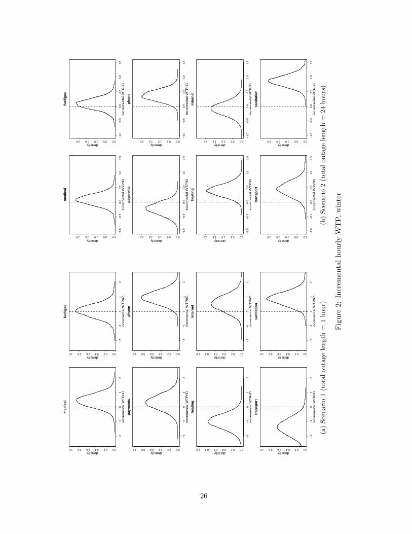
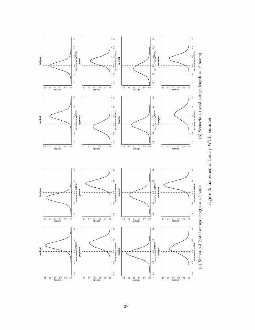
equations. Fortunately, scenario effects emerge as irrelevant for the two winter equations.10

Our main focus, however, rests with the IS indicators, captured in the second-to-last

block of rows of the table. Most noteworthy, concerns about failure in communication

(“phone”) and water and sanitation (“sanitation”) services increase WTP in all four cases.

These are also the only significant IS effects for the shorter winter outage. Not surpris-

10We re-estimated our model for the two sub-samples associated with a given scenario ordering. Whilemodel coefficients change somewhat with the loss of 50% of our sample, the IS effects, which are the centralfocus of our analysis, remain qualitatively similar for both groups and compared to the full sample. Thatis, essentially the same ISs emerge as important for a given outage scenario in all three specifications.

24

ingly, the three longer outages all produce additional IS effects with the bulk of posterior

mass above zero. Specifically, for the winter, 24 hour case heating and transportation are

of primary concern, while a possible disruption of medical services produces significant

results for both summer scenarios. In addition, “payments” emerge as significant for the

shorter summer outage, while “transport” plays an important role for the summer, 12 hours

interruption.11

Figures 1 and 2 depict these IS results in graphic form. Figure 1 shows the posterior

distribution of the marginal IS effects on average hourly WTP for the two winter scenarios,

while figure 2 provides the analog for the summer interruptions. A dotted vertical zero-line

is superimposed on each sub-figure. As can be seen from these graphs, the marginal IS

effects identified as significant in the above discussion all have posterior distributions that

lie almost exclusively to the right of zero.

Thus, as the main result of our study, we conclude that there exist indeed a separate

IS effects within households’ overall WTP to avoid a power outages. Furthermore, these

effects are non-trivial in magnitude, with posterior expectations ranging from e0.3/hour to

close to e1/hour. Recall that these figures are best interpreted as lower bounds given our

data limitations. In order to put these estimates in perspective to overall WTP, we now

proceed to our predictive welfare analysis.

3.3 Predicted WTP

We derive posterior predictive distributions for each scenario and country for the following

three settings of IS indicators: (i) as observed in the actual sample (“actual”), (ii) all indi-

cators set to one (counterfactual belief that all of the services are impacted, “all affected”),

and all to set to zero (counterfactual belief that none of the services are impacted, “none

affected”). The last metric thus produces benchmark estimates for WTP related exclusively

to the loss of front-door electricity, net of (likely minor) savings due to non-use of appli-

11In contrast, transportation has a counter-intuitive significant negative effect on WTP for the one hourwinter outage. This is likely due to the fact that some respondents that believed transportation serviceswould be affected for a longer interruption did not hold this concern for this short outage. As mentionedabove, this would bias the corresponding coefficient downwards.

25

−2

−1

01

2

0.00.20.40.60.81.0

med

ical

incr

emen

tal W

TP

(€)

density

−2

−1

01

2

0.00.20.40.60.81.0

fuel

/gas

incr

emen

tal W

TP

(€)

density

−2

−1

01

2

0.00.20.40.60.81.0

paym

ents

incr

emen

tal W

TP

(€)

density

−2

−1

01

2

0.00.20.40.60.81.0

phon

e

incr

emen

tal W

TP

(€)

density

−2

−1

01

2

0.00.20.40.60.81.0

heat

ing

incr

emen

tal W

TP

(€)

density

−2

−1

01

2

0.00.20.40.60.81.0

inte

rnet

incr

emen

tal W

TP

(€)

density

−2

−1

01

2

0.00.20.40.60.81.0

tran

spor

t

incr

emen

tal W

TP

(€)

density

−2

−1

01

2

0.00.20.40.60.81.0

sani

tatio

n

incr

emen

tal W

TP

(€)

density

(a)

Sce

nar

io1

(tot

alou

tage

len

gth

=1

hou

r)

−1.

0−

0.5

0.0

0.5

1.0

1.5

0.00.51.01.52.0

med

ical

incr

emen

tal W

TP

(€)

density

−1.

0−

0.5

0.0

0.5

1.0

1.5

0.00.51.01.52.0

fuel

/gas

incr

emen

tal W

TP

(€)

density

−1.

0−

0.5

0.0

0.5

1.0

1.5

0.00.51.01.52.0

paym

ents

incr

emen

tal W

TP

(€)

density

−1.

0−

0.5

0.0

0.5

1.0

1.5

0.00.51.01.52.0

phon

e

incr

emen

tal W

TP

(€)

density

−1.

0−

0.5

0.0

0.5

1.0

1.5

0.00.51.01.52.0

heat

ing

incr

emen

tal W

TP

(€)

density

−1.

0−

0.5

0.0

0.5

1.0

1.5

0.00.51.01.52.0

inte

rnet

incr

emen

tal W

TP

(€)

density

−1.

0−

0.5

0.0

0.5

1.0

1.5

0.00.51.01.52.0

tran

spor

t

incr

emen

tal W

TP

(€)

density

−1.

0−

0.5

0.0

0.5

1.0

1.5

0.00.51.01.52.0

sani

tatio

n

incr

emen

tal W

TP

(€)

density

(b)

Sce

nari

o2

(tota

lou

tage

len

gth

=24

hou

rs)

Fig

ure

2:In

crem

enta

lh

ourl

yW

TP

,w

inte

r

26

−1.

0−

0.5

0.0

0.5

1.0

0.00.51.01.52.02.5

med

ical

incr

emen

tal W

TP

(€)

density

−1.

0−

0.5

0.0

0.5

1.0

0.00.51.01.52.02.5

fuel

/gas

incr

emen

tal W

TP

(€)

density

−1.

0−

0.5

0.0

0.5

1.0

0.00.51.01.52.02.5

paym

ents

incr

emen

tal W

TP

(€)

density

−1.

0−

0.5

0.0

0.5

1.0

0.00.51.01.52.02.5

phon

e

incr

emen

tal W

TP

(€)

density

−1.

0−

0.5

0.0

0.5

1.0

0.00.51.01.52.02.5

heat

ing

incr

emen

tal W

TP

(€)

density

−1.

0−

0.5

0.0

0.5

1.0

0.00.51.01.52.02.5

inte

rnet

incr

emen

tal W

TP

(€)

density

−1.

0−

0.5

0.0

0.5

1.0

0.00.51.01.52.02.5

tran

spor

t

incr

emen

tal W

TP

(€)

density

−1.

0−

0.5

0.0

0.5

1.0

0.00.51.01.52.02.5

sani

tatio

n

incr

emen

tal W

TP

(€)

density

(a)

Sce

nar

io3

(tot

alou

tage

len

gth

=4

hou

rs)

−1.

0−

0.5

0.0

0.5

1.0

1.5

0.00.51.01.52.02.5

med

ical

incr

emen

tal W

TP

(€)

density

−1.

0−

0.5

0.0

0.5

1.0

1.5

0.00.51.01.52.02.5

fuel

/gas

incr

emen

tal W

TP

(€)

density

−1.

0−

0.5

0.0

0.5

1.0

1.5

0.00.51.01.52.02.5

paym

ents

incr

emen

tal W

TP

(€)

density

−1.

0−

0.5

0.0

0.5

1.0

1.5

0.00.51.01.52.02.5

phon

e

incr

emen

tal W

TP

(€)

density

−1.

0−

0.5

0.0

0.5

1.0

1.5

0.00.51.01.52.02.5

heat

ing

incr

emen

tal W

TP

(€)

density

−1.

0−

0.5

0.0

0.5

1.0

1.5

0.00.51.01.52.02.5

inte

rnet

incr

emen

tal W

TP

(€)

density

−1.

0−

0.5

0.0

0.5

1.0

1.5

0.00.51.01.52.02.5

tran

spor

t

incr

emen

tal W

TP

(€)

density

−1.

0−

0.5

0.0

0.5

1.0

1.5

0.00.51.01.52.02.5

sani

tatio

n

incr

emen

tal W

TP

(€)

density

(b)

Sce

nari

o4

(tota

lou

tage

len

gth

=12

hou

rs)

Fig

ure

3:In

crem

enta

lh

ourl

yW

TP

,su

mm

er

27

ances. In all three cases predicted WTP estimates are averaged over all individuals within

a given country.

Numerical results are given in table 9 in appendix B. The first block of rows shows

within-sample predictions based on actually observed beliefs about IS impact. Thus, these

estimates combine front-door and IS-related values, as one would obtain without explicitly

distinguishing between the two components in the first place. As is evident from the table,

average hourly WTP is clearly positive for all country-scenario combinations, and generally

larger in winter than in summer. Interestingly, average hourly WTP is generally lower for

the longer winter outage compared to the shorter winter scenario, but higher for the longer

summer outage compared to the shorter summer interruption. This suggests decreasing

marginal costs over duration (perhaps due to gradual adaptation), and increasing marginal

costs in summer (perhaps due increasing food losses due to spoilage). Overall, hourly WTP

in winter lies in the e1.50 - e4.2 range, compared to a range of e0.20 - e2.1 for the summer.

The second block of rows shows posterior results for predicted WTP, with all IS indi-

cators set to one. This leads to an unambiguous increase in values for all scenario-country

combinations, with hourly estimates now lying in the e2.2 - e5.0 range for winter, and in

the e0.5 - e2.7 range for summer. Conversely, WTP bare any IS effects, as captured in

the last block of rows is markedly reduced compared to the within-sample, especially for

the three outages lasting longer than one hour. In fact, with few exceptions (Denmark,

Luxembourg) WTP becomes statistically indistinguishable from zero for the two summer

outages once we abstract from IS impacts.12

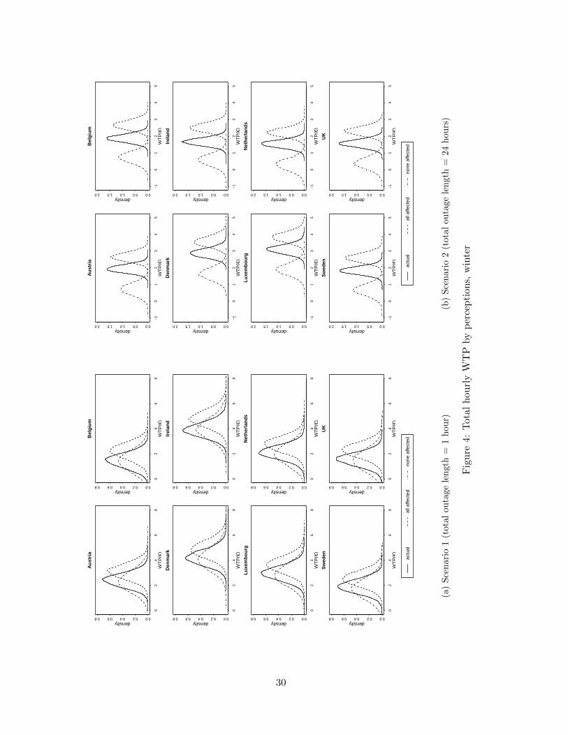
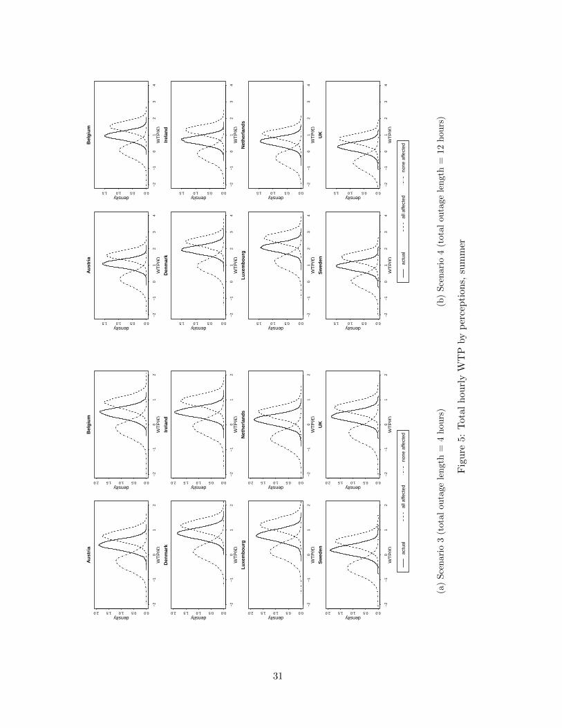
Figures 4, for winter, and 5 for summer present a graphical representation of these

posterior predictive distributions (PPDs). Each subplot shows the PPD of the within-

sample (“actual”) predictions, with the PPDs for “none affected” and “all affected” super-

imposed for each case. As is evident from figure 4, there is considerable overlap of the three

distributions for the one-hour interruption for all eight countries. This is not surprising,

12Our linear model leaves the support of predicted WTP unrestricted, which produces negative entriesfor several posterior means for the summer interruptions. We also estimated our model with latent WTP inlog form to restrict predictions to the positive domain. However, with only three to four bids per scenario,the tails of the implicit log-normal distributions are poorly characterized. This leads to excessive posteriormeans for predicted WTP. We therefore opt to use the linear model for inference.

28

as IS impacts will likely be a relatively minor concern for such short interruptions for the

typical resident. In contrast, the “none affected” and “all affected” densities are clearly

pulled apart for the 24 hour winter outage. The same holds for both summer interruptions

(figure 5). Thus, our predictive analysis lends additional evidence to the fact that total WTP

to avoid a residential outage includes a sizable, and potentially dominating IS component.

Reassuringly, our WTP estimate for the one-hour winter outage for Sweden for the “none

affected” counterfactual (e1.72) lies within 30% of the estimate produced by Carlsson and

Martinsson (2007) based on their Swedish 2004 data for a winter scenario of equal length,

but occurring earlier in the evening (6 pm compared to 8 pm in our case). When converted to

euros and adjusted for inflation their estimate amounts to e2.42. In that study, the authors

took great care to stress to respondents that payment of the proposed bid would only guard

against front-door losses, so our “none affected” result is the appropriate measure stick for

comparison. The residual gap between the two estimates is likely due to the difference

in the stipulated time of onset for the interruption and potential shifts in preferences of

power provision over the decade that separates their data from ours. Reichl et al. (2013)

report an average hourly WTP of e1.9 across all of their outage scenarios for their 2009

sample of Austrian households, which varied in season and duration in similar fashion to

our design. In their analysis, respondents were directly instructed to expect IS failures

when making a payment decision. Thus, the most relevant measure for comparison are our

hourly predictions from the “all affected” counterfactual, which, for Austria, range from

e0.8 (summer, four hours) to e3.1 (winter, one hour), and thus bracket Reichl et al.’s

aggregate result, as expected.

To gain a sense of the relative proportions of WTP related to front-door losses and

values related to disrupted IS services we compute IS values as percentage of total WTP

and as percentage of front-door WTP for all IS services that emerged as significant for a

given scenario for the full sample of households. For the comparison relative to front-door

WTP can only use winter scenarios since, as discussed above, the benchmark WTP for

front-door effects is essentially zero for summer interruptions and the typical household.

The resulting percentages are captured in table 5. In terms of overall hourly WTP, the

29

02

46

8

0.00.20.40.60.8

Aus

tria

WT

P(€

)

density

02

46

8

0.00.20.40.60.8

Bel

gium

WT

P(€

)

density

02

46

8

0.00.20.40.60.8

Den

mar

k

WT

P(€

)

density

02

46

8

0.00.20.40.60.8

Irel

and

WT

P(€

)density

02

46

8

0.00.20.40.60.8

Luxe

mbo

urg

WT

P(€

)

density

02

46

8

0.00.20.40.60.8N

ethe

rland

s

WT

P(€

)

density

02

46

8

0.00.20.40.60.8

Sw

eden

WT

P(€

)

density

02

46

8

0.00.20.40.60.8

UK

WT

P(€

)

density

actu

alal

l affe

cted

none

affe

cted

(a)

Sce

nar

io1

(tot

alou

tage

len

gth

=1

hou

r)

−1

01

23

45

0.00.51.01.52.0

Aus

tria

WT

P(€

)

density

−1

01

23

45

0.00.51.01.52.0

Bel

gium

WT

P(€

)

density

−1

01

23

45

0.00.51.01.52.0

Den

mar

k

WT

P(€

)

density

−1

01

23

45

0.00.51.01.52.0

Irel

and

WT

P(€

)

density

−1

01

23

45

0.00.51.01.52.0

Luxe

mbo

urg

WT

P(€

)

density

−1

01

23

45

0.00.51.01.52.0

Net

herla

nds

WT

P(€

)

density

−1

01

23

45

0.00.51.01.52.0

Sw

eden

WT

P(€

)

density

−1

01

23

45

0.00.51.01.52.0

UK

WT

P(€

)

density

actu

alal

l affe

cted

none

affe

cted

(b)

Sce

nari

o2

(tota

lou

tage

len

gth

=24

hou

rs)

Fig

ure

4:T

otal

hou

rly

WT

Pby

per

cep

tion

s,w

inte

r

30

−2

−1

01

2

0.00.51.01.52.0

Aus

tria

WT

P(€

)

density

−2

−1

01

2

0.00.51.01.52.0

Bel

gium

WT

P(€

)

density

−2

−1

01

2

0.00.51.01.52.0

Den

mar

k

WT

P(€

)

density

−2

−1

01

2

0.00.51.01.52.0

Irel

and

WT

P(€

)density

−2

−1

01

2

0.00.51.01.52.0

Luxe

mbo

urg

WT

P(€

)

density

−2

−1

01

2

0.00.51.01.52.0N

ethe

rland

s

WT

P(€

)

density

−2

−1

01

2

0.00.51.01.52.0

Sw

eden

WT

P(€

)

density

−2

−1

01

2

0.00.51.01.52.0

UK

WT

P(€

)

density

actu

alal

l affe

cted

none

affe

cted

(a)

Sce

nar

io3

(tot

alou

tage

len

gth

=4

hou

rs)

−2

−1

01

23

4

0.00.51.01.5

Aus

tria

WT

P(€

)

density

−2

−1

01

23

4

0.00.51.01.5

Bel

gium

WT

P(€

)

density

−2

−1

01

23

4

0.00.51.01.5

Den

mar

k

WT

P(€

)

density

−2

−1

01

23

4

0.00.51.01.5

Irel

and

WT

P(€

)

density

−2

−1

01

23

4

0.00.51.01.5

Luxe

mbo

urg

WT

P(€

)

density

−2

−1

01

23

4

0.00.51.01.5

Net

herla

nds

WT

P(€

)

density

−2

−1

01

23

4

0.00.51.01.5

Sw

eden

WT

P(€

)

density

−2

−1

01

23

4

0.00.51.01.5

UK

WT

P(€

)

density

actu

alal

l affe

cted

none

affe

cted

(b)

Sce

nari

o4

(tota

lou

tage

len

gth

=12

hou

rs)

Fig

ure

5:T

otal

hou

rly

WT

Pby

per

cep

tion

s,su

mm

er

31

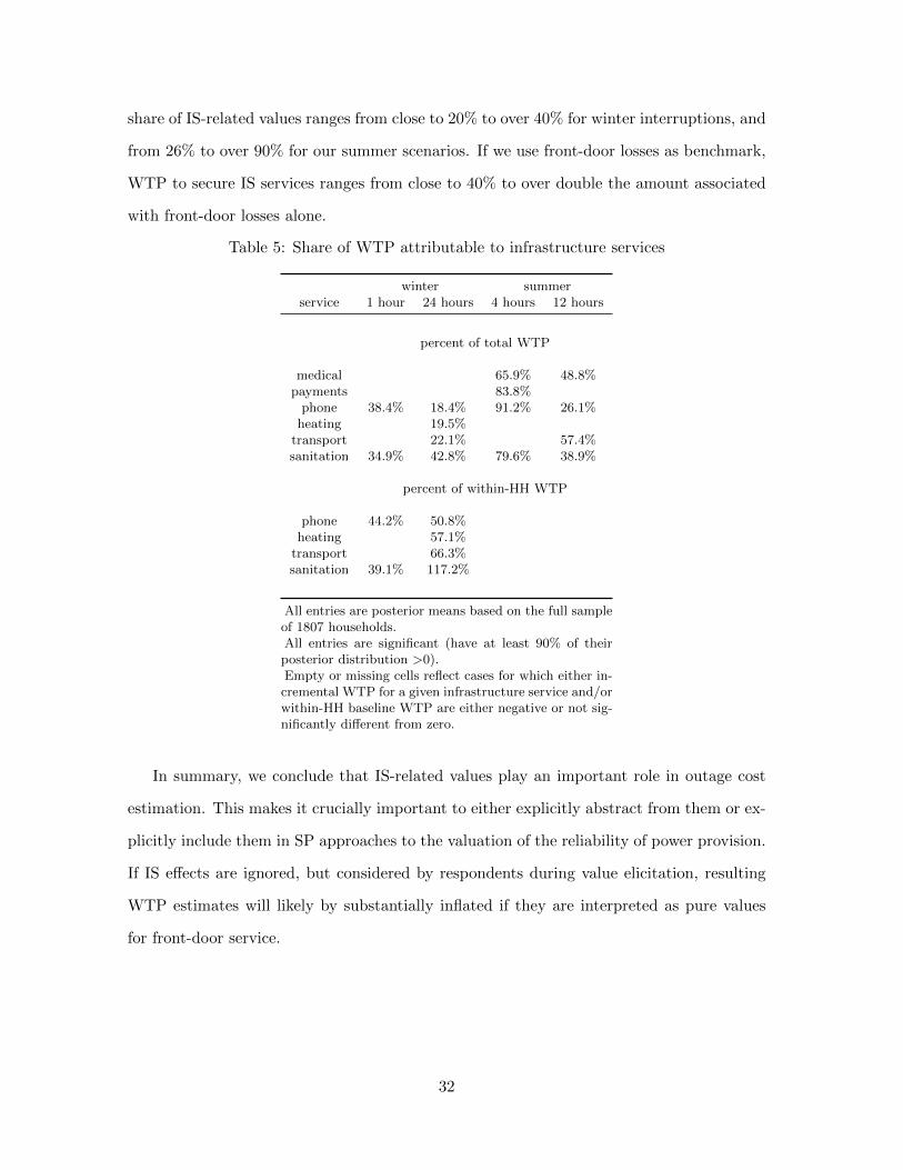
share of IS-related values ranges from close to 20% to over 40% for winter interruptions, and

from 26% to over 90% for our summer scenarios. If we use front-door losses as benchmark,

WTP to secure IS services ranges from close to 40% to over double the amount associated

with front-door losses alone.

Table 5: Share of WTP attributable to infrastructure services

winter summerservice 1 hour 24 hours 4 hours 12 hours

percent of total WTP

medical 65.9% 48.8%payments 83.8%

phone 38.4% 18.4% 91.2% 26.1%heating 19.5%

transport 22.1% 57.4%sanitation 34.9% 42.8% 79.6% 38.9%

percent of within-HH WTP

phone 44.2% 50.8%heating 57.1%

transport 66.3%sanitation 39.1% 117.2%

All entries are posterior means based on the full sampleof 1807 households.All entries are significant (have at least 90% of theirposterior distribution >0).Empty or missing cells reflect cases for which either in-cremental WTP for a given infrastructure service and/orwithin-HH baseline WTP are either negative or not sig-nificantly different from zero.

In summary, we conclude that IS-related values play an important role in outage cost

estimation. This makes it crucially important to either explicitly abstract from them or ex-

plicitly include them in SP approaches to the valuation of the reliability of power provision.

If IS effects are ignored, but considered by respondents during value elicitation, resulting

WTP estimates will likely by substantially inflated if they are interpreted as pure values

for front-door service.

32

4 Conclusion

This study shows how the essential-input property of electricity in the provision of household

commodities can be exploited to dis-entangle welfare effects related to power delivered

to the “front door” from values related to the disruption of vital infrastructure services.

Specifically, we illustrate how the popular surplus model based on Random Utility Theory

flows naturally from a household production framework with electricity playing the central

role of an essential input. Using a survey-based identification strategy, we partition total

WTP to avoid a specific power interruption into front-door and IS effects.

Though our welfare estimates for ISs can only be interpreted as lower bounds given the

limitations of our empirical data, our findings provide strong evidence that a considerable

portion of total WTP to avoid an outage relates to the loss of public services. We find our

sample of households from eight EU nations to be especially sensitive to a disruption of med-

ical, communication, transportation, and sanitation services. This stresses the importance

of explicitly specifying the scale of outages and their expected impact on IS components in

SP elicitation. Either a convincing statement needs to be made to respondents that stipu-

lated outages are highly localized, leaving ISs unaffected, or survey participants should be

prompted to think about IS impacts (or given information on potential IS effects) when

confronted with interruption scenarios that cover a larger spatial scale. Failure to do so will

produce welfare estimates that are unfit to inform policy.

From a public policy perspective, our findings are perhaps best interpreted as strong

evidence that a widespread loss of power harms residential customers through more than

just the interruption of front-door service. Protecting vital elements of the public infras-

tructure may be just as important, if not more so, than assuring adequate power flow to

the neighborhood grid. From a EU standpoint our findings stress the importance of the

planned expansion of the electric transmission network to improve inter-regional connec-

tivity and grid reliability, since large-scale, IS-impacting outages are frequently caused by

transmission failures (Buldyrev et al., 2010; European Commission, 2012; ENTSO-E, 2012).

Taking our results as a first indication, the welfare gains from increased reliability of power

33

provision due to a strengthening of the transmission grid could be potentially much larger

than one would conclude from past valuation studies that only focused on front-door effects,

especially in light of increasing threats to the grid due to climate change.

Our findings also raise concerns surrounding the use of normalized outage costs based on

“WTP/kwh unserved” to facilitate inter-study comparison (e.g. Doane et al., 1988a,b; Woo

et al., 1991; Beenstock et al., 1998; Layton and Moeltner, 2005; Carlsson and Martinsson,

2007). For this common metric “unserved” refers to the front-door load that would have

been normally consumed by the household in absence of a given interruption. However, in

cases where the scale of a hypothetical interruption is left to the guess of the respondent,

such WTP/kwh estimates will be misleading, since WTP may refer to much broader dam-

ages than those that could be fixed by leaving front-door service intact. Specifically, if WTP

comprises IS components but WTP/kwh is meant to apply exclusively to front-door losses

and consumption, the numerator and thus the entire fraction will be inflated. If WTP/kwh

is meant to hold for all losses (front-door plus IS) the denominator would have to be com-

puted as the sum of front-door consumption plus per-capita electricity consumption that

would have fed into IS’s for the metric to have any meaningful interpretation.

Naturally, our study is best thought of as a starting point for a more in-depth anal-

ysis of infrastructure values, using hypothetical choice experiments on power outages as

identification vehicle. Our modest sample sizes and lack of hierarchical depth in our data

layers preempts any examination of individual or even country-level heterogeneity in IS-

related preferences. Furthermore, it would be desirable in subsequent research to ask the

IS-perception question for each stipulated outage, perhaps with more detailed probing of

how exactly loss-of-service would affect the household. A more surgical approach could

also be taken by focusing exclusively on a single IS, for example public transportation, and

assuring respondents that other ISs would remain unaffected. This could be further devel-

oped to allow for quality changes in service, instead of or in addition to the all-or-nothing

condition implicit in our scenarios.

At a more general level, our study provides insights on the broader economic values at

stake if the electricity sector is not protected against the increasing threats related to climate

34

change. It also offers a glimpse into the direct values-at-risk related to other infrastructure

services, thus adding to the “limited set of published studies” that have examined the

potential impacts of climate change on public services using a quantitative approach Arent

et al. (2014). While adaptive measures will need to be taken to increase the resilience of

all of these elements of the public infrastructure, the power grid clearly deserves special

attention due to the essential input property of electricity.

35

Appendix A: Infrastructure perception question

page 2/13

TABLE 1 - Effects of power outage on infrastructure and facilities

Consider an outage that started 4 hours ago. How do you think the following are affected?

Not at all affected

(1)

Moderately affected

(2)

Strongly affected

(3)

Very strongly affected

(4)

Affected parts of society and Infrastructure

Row

Medical Care (first responders, hospitals,…)

1

Fuel/ Gas supply (cars, buses, emergency responders, heating, fuel …)

2

Electronic Payment Options (ATMs, credit cards, transfers,…)

3

Land Line & Mobile Telephone networks (communication, emergency calls,…)

4

Heating Systems (require electric controls/pumps)

5

Internet & network connections (email, internet, etc.)

6

Electrically operated traffic (e.g. public transport, metro,…)

7

Sanitation & sewage treatment (water supply, hygiene,..)

8

36

Appendix B: Additional Tables

37

Tab

le6:

Bid

s(e

uro

s)an

d%

“yes

”re

spon

ses

by

scen

ario

and

cou

ntr

y

scen

ari

o1

(win

ter,

1h

ou

r)sc

enari

o2

(win

ter,

24

hou

rs)

cou

ntr

yb

id1

bid

2b

id3

bid

4%

yes

1%

yes

2%

yes

3%

yes

4b

id1

bid

2b

id3

bid

4%

yes

1%

yes

2%

yes

3%

yes

4

Au

stri

a0.2

53.0

05.0

0-

65.3

240.0

035.3

9-

8.0

040.0

070.0

0-

77.3

638.7

141.9

4-

Bel

giu

m0.2

53.0

05.0

0-

60.9

530.7

733.3

3-

7.0

08.0

038.0

070.0

075.4

471.1

544.4

439.2

2D

enm

ark

0.2

73.3

65.3

7-

76.4

250.0

038.1

8-

8.0

58.7

246.9

869.8

076.9

281.8

260.3

854.7

2Ir

elan

d0.2

53.0

05.0

0-

72.5

059.2

637.7

0-

7.0

08.0

038.0

070.0

085.2

574.0

742.1

120.6

3L

uxem

bou

rg0.2

55.0

0-

-63.1

141.7

5-

-8.0

011.0

066.0

070.0

084.6

280.3

945.1

059.6

2N

eth

erla

nd

s0.2

53.0

05.0

0-

64.3

535.1

936.0

7-

8.0

040.0

070.0

0-

69.5

731.1

542.5

9-

Sw

eden

0.2

32.9

05.2

2-

65.5

737.7

424.1

4-

8.1

240.5

971.9

0-

72.9

743.7

541.3

8-

UK

0.3

12.5

04.9

5-

62.8

038.1

027.8

7-

6.1

78.6

435.8

176.6

173.7

768.2

545.9

028.3

3

scen

ari

o3

(su

mm

er,

4h

ou

rs)

scen

ari

o4

(su

mm

er,

12

hou

rs)

cou

ntr

yb

id1

bid

2b

id3

bid

4%

yes

1%

yes

2%

yes

3%

yes

4b

id1

bid

2b

id3

bid

4%

yes

1%

yes

2%

yes

3%

yes

4A

ust

ria

0.5

01.0

07.0

09.0

053.2

260.0

024.1

923.5

35.0

020.0

025.0

045.0

059.6

837.1

037.2

521.8

1B

elgiu

m0.5

01.0

07.0

09.0

062.7

546.1

524.0

731.5

85.0

019.0

024.0

045.0

062.9

643.1

428.0

721.1

5D

enm

ark

0.5

41.0

78.0

58.7

267.9

253.8

532.0

827.2

75.3

724.1

629.5

344.9

769.8

150.9

443.6

425.0

0Ir

elan

d0.5

01.0

07.0

09.0

053.9

764.8

128.0

716.3

95.0

019.0

024.0

045.0

061.4

026.9

834.4

312.9

6L

uxem

bou

rg0.5

01.0

09.0

012.0

057.6

955.7

733.3

319.6

15.0

033.0

041.0

045.0

068.6

336.5

435.2

936.5

4N

eth

erla

nd

s0.5

01.0

07.0

09.0

062.9

648.1

514.7

518.0

35.0

020.0

025.0

045.0

054.1

044.4

424.5

914.8

1S

wed

en0.5

80.9

36.9

69.2

855.1

749.0

623.4

418.9

75.2

219.7

125.5

146.3

954.6

948.2

825.8

618.8

7U

K0.6

26.1

79.8

8-

63.4

116.3

914.7

5-

4.9

418.5

222.2

246.9

254.1

033.3

322.9

514.2

8

38

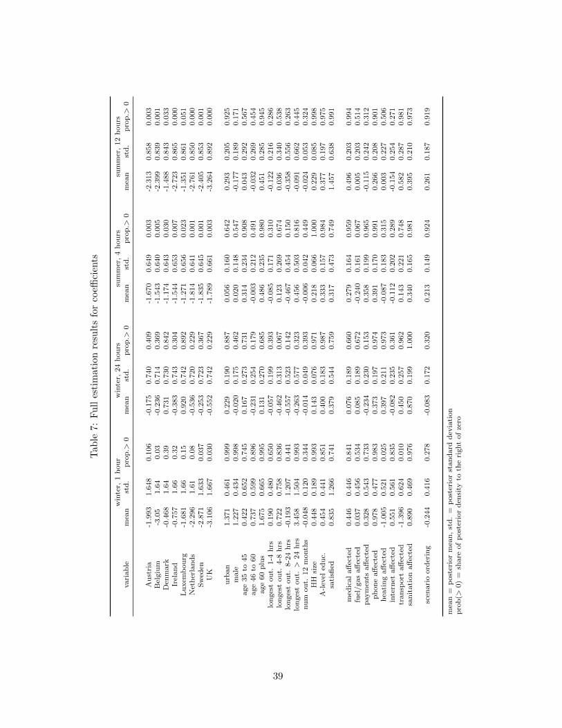
Tab

le7:

Fu

lles

tim

atio

nre

sult

sfo

rco

effici

ents

win

ter,

1h

ou

rw

inte

r,24

hou

rssu

mm

er,

4h

ou

rssu

mm

er,

12

hou

rsvari

ab

lem

ean

std

.p

rop

.>0

mea

nst

d.

pro

p.>

0m

ean

std

.p

rop

.>0

mea

nst

d.

pro

p.>

0

Au

stri

a-1

.993

1.6

48

0.1

06

-0.1

75

0.7

40

0.4

09

-1.6

70

0.6

49

0.0

03

-2.3

13

0.8

58

0.0

03

Bel

giu

m-3

.05

1.6

40.0

3-0

.236

0.7

14

0.3

69

-1.5

43

0.6

40

0.0

05

-2.3

99

0.8

39

0.0

01

Den

mark

-0.4

68

1.6

40.3

90.7

31

0.7

30

0.8

42

-1.1

74

0.6

43

0.0

30

-1.4

88

0.8

43

0.0

33

Irel

an

d-0

.757

1.6

60.3

2-0

.383

0.7

43

0.3

04

-1.5

44

0.6

53

0.0

07

-2.7

23

0.8

65

0.0

00

Lu

xem

bou

rg-1

.681

1.6

60.1

50.9

20

0.7

42

0.8

92

-1.2

71

0.6

56

0.0

23

-1.3

51

0.8

61

0.0

51

Net

her

lan

ds

-2.2

96

1.6

10.0

8-0

.536

0.7

20

0.2

29

-1.8

14

0.6

41

0.0

01

-2.7

61

0.8

50

0.0

00

Sw

eden

-2.8

71

1.6

33

0.0

37

-0.2

53

0.7

23

0.3

67

-1.8

35

0.6

45

0.0

01

-2.4

05

0.8

53

0.0

01

UK

-3.1

06

1.6

67

0.0

30

-0.5

52

0.7

42

0.2

29

-1.7

89

0.6

61

0.0

03

-3.2

64

0.8

92

0.0

00

urb

an

1.3

71

0.4

61

0.9

99

0.2

29

0.1

90

0.8

87

0.0

56

0.1

60

0.6

42

0.2

93

0.2

05

0.9

25

male

1.2

27

0.4

34

0.9

98

-0.0

20

0.1

75

0.4

62

0.0

20

0.1

48

0.5

47

-0.1

77

0.1

89

0.1

71

age

35

to45

0.4

22

0.6

52

0.7

45

0.1

67

0.2

73

0.7

31

0.3

14

0.2

34

0.9

08

0.0

43

0.2

92

0.5

67

age

46

to60

0.7

37

0.5

99

0.8

96

-0.2

31

0.2

54

0.1

79

-0.0

03

0.2

12

0.4

91

-0.0

32

0.2

69

0.4

54

age

60

plu

s1.6

75

0.6

65

0.9

95

0.1

31

0.2

70

0.6

85

0.4

86

0.2

35

0.9

80

0.4

51

0.2

85

0.9

45

lon

ges

tou

t.1-4

hrs

0.1

90

0.4

80

0.6

50

-0.0

57

0.1

99

0.3

93

-0.0

85

0.1

71

0.3

10

-0.1

22

0.2

16

0.2

86

lon

ges

tou

t.4-8

hrs

0.7

22

0.7

58

0.8

36

-0.4

62

0.3

13

0.0

67

0.1

23

0.2

69

0.6

74

0.0

36

0.3

40

0.5

38

lon

ges

tou

t.8-2

4h

rs-0

.193

1.2

07

0.4

41

-0.5

57

0.5

23

0.1

42

-0.4

67

0.4

54

0.1

50

-0.3

58

0.5

56

0.2

63

lon

ges

tou

t.>

24

hrs

3.4

58

1.5

04

0.9

93

-0.2

63

0.5

77

0.3

23

0.4

56

0.5

03

0.8

16

-0.0

91

0.6

62

0.4

45

num

ou

t.12

month

s-0

.048

0.1

20

0.3

44

-0.0

14

0.0

49

0.3

93

-0.0

06

0.0

42

0.4

49

-0.0

24

0.0

53

0.3

24

HH

size

0.4

48

0.1

89

0.9

93

0.1

43

0.0

76

0.9

71

0.2

18

0.0

66

1.0

00

0.2

29

0.0

85

0.9

98

A-l

evel

edu

c.0.4

54

0.4

41

0.8

51

0.4

00

0.1

83

0.9

87

0.3

33

0.1

57

0.9

84

0.3

77

0.1

97

0.9

75

sati

sfied

0.8

35

1.2

66

0.7

41

0.3

79

0.5

44

0.7

59

0.3

17

0.4

73

0.7

49

1.4

57

0.6

38

0.9

91

med

ical

aff

ecte

d0.4

46

0.4

46

0.8

41

0.0

76

0.1

89

0.6

60

0.2

79

0.1

64

0.9

59

0.4

96

0.2

03

0.9

94

fuel

/gas

aff

ecte

d0.0

37

0.4

56

0.5

34

0.0

85

0.1

89

0.6

72

-0.2

40

0.1

61

0.0

67

0.0

05

0.2

03

0.5

14

paym

ents

aff

ecte

d0.3

28

0.5

43

0.7

33

-0.2

34

0.2

30

0.1

53

0.3

58

0.1

99

0.9

65

-0.1

15

0.2

42

0.3

12

ph

on

eaff

ecte

d0.9

78

0.4

77

0.9

83

0.3

73

0.1

97

0.9

74

0.3

91

0.1

70

0.9

91

0.2

66

0.2

08

0.9

01

hea

tin

gaff

ecte

d-1

.005

0.5

21

0.0

25

0.3

97

0.2

11

0.9

73

-0.0

87

0.1

83

0.3

15

0.0

03

0.2

27

0.5

06

inte

rnet

aff

ecte

d0.5

51

0.5

61

0.8

35

-0.0

82

0.2

35

0.3

61

-0.1

12

0.2

02

0.2

89

-0.1

54

0.2

54

0.2

71

tran

sport

aff

ecte

d-1

.396

0.6

24

0.0

10

0.4

50

0.2

57

0.9

62

0.1

43

0.2

21

0.7

48

0.5

82

0.2

87

0.9

81

san

itati

on

aff

ecte

d0.8

90

0.4

69

0.9

76

0.8

70

0.1

99

1.0

00

0.3

40

0.1

65

0.9

81

0.3

95

0.2

10

0.9

73

scen

ari

oord

erin

g-0

.244

0.4

16

0.2

78

-0.0

83

0.1

72

0.3

20

0.2

13

0.1

49

0.9

24

0.2

61

0.1

87

0.9

19

mea

n=

post

erio

rm

ean

,st

d.

=p

ost

erio

rst

an

dard

dev

iati

on

pro

b(>

0)

=sh

are

of

post

erio

rd

ensi

tyto

the

right

of

zero

39

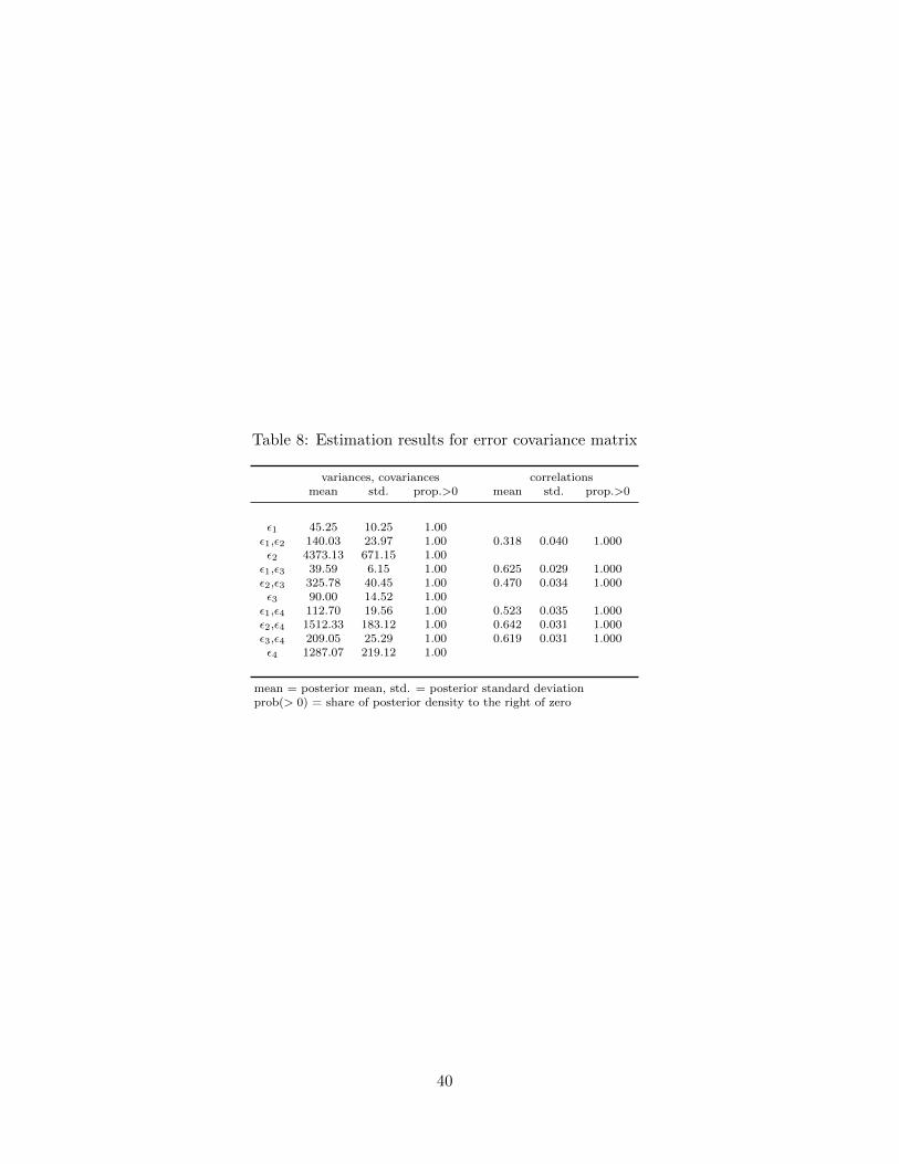
Table 8: Estimation results for error covariance matrix

variances, covariances correlationsmean std. prop.>0 mean std. prop.>0

ε1 45.25 10.25 1.00ε1,ε2 140.03 23.97 1.00 0.318 0.040 1.000ε2 4373.13 671.15 1.00ε1,ε3 39.59 6.15 1.00 0.625 0.029 1.000ε2,ε3 325.78 40.45 1.00 0.470 0.034 1.000ε3 90.00 14.52 1.00ε1,ε4 112.70 19.56 1.00 0.523 0.035 1.000ε2,ε4 1512.33 183.12 1.00 0.642 0.031 1.000ε3,ε4 209.05 25.29 1.00 0.619 0.031 1.000ε4 1287.07 219.12 1.00

mean = posterior mean, std. = posterior standard deviationprob(> 0) = share of posterior density to the right of zero

40

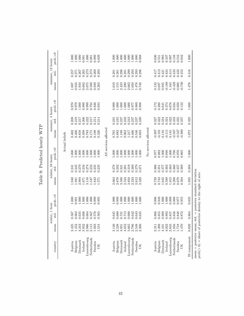
Tab

le9:

Pre

dic

ted

hou

rly

WT

P

win

ter,

1h

ou

rw

inte

r,24

hou

rssu

mm

er,

4h

ou

rssu

mm

er,

12

hou

rsco

untr

ym

ean

std

.p

rob

.>0

mea

nst

d.

pro

b.>

0m

ean

std

.p

rob

.>0

mea

nst

d.

pro

b.>

0

Act

ual

bel

iefs

Au

stri

a2.4

25

0.5

67

1.0

00

1.9

48

0.2

41

1.0

00

0.4

02

0.2

09

0.9

70

1.0

87

0.2

57

1.0

00

Bel

giu

m1.4

52

0.6

04

0.9

91

1.8

81

0.2

45

1.0

00

0.4

66

0.2

19

0.9

79

0.9

44

0.2

71

1.0

00

Den

mark

4.2

43

0.6

35

1.0

00

2.8

94

0.2

79

1.0

00

0.8

58

0.2

17

1.0

00

1.9

34

0.2

67

1.0

00

Irel

an

d3.9

32

0.6

06

1.0

00

1.6

71

0.2

34

1.0

00

0.4

98

0.2

06

0.9

90

0.6

82

0.2

65

0.9

91

Lu

xem

bou

rg2.9

86

0.6

04

1.0

00

3.1

16

0.2

74

1.0

00

0.7

83

0.2

22

0.9

99

2.0

75

0.2

73

1.0

00

Net

her

lan

ds

2.1

15

0.5

67

1.0

00

1.5

47

0.2

33

1.0

00

0.1

75

0.2

17

0.7

94

0.5

89

0.2

73

0.9

81

Sw

eden

1.9

23

0.5

70

0.9

99

1.8

43

0.2

35

1.0

00

0.1

98

0.2

14

0.8

26

0.9

39

0.2

69

0.9

99

UK

1.5

54

0.5

65

0.9

95

1.5

71

0.2

35

1.0

00

0.3

26

0.2

14

0.9

34

0.2

63

0.2

83

0.8

29

All

serv

ices

aff

ecte

d

Au

stri

a3.1

40

0.6

45

1.0

00

2.6

64

0.2

78

1.0

00

0.7

65

0.2

31

0.9

99

1.6

10

0.2

81

1.0

00

Bel

giu

m2.2

28

0.6

80

0.9

99

2.6

78

0.2

92

1.0

00

0.8

82

0.2

45

1.0

00

1.5

15

0.3

01

1.0

00

Den

mark

4.9

31

0.7

21

1.0

00

3.5

80

0.3

21

1.0

00

1.1

88

0.2

37

1.0

00

2.4

23

0.2

96

1.0

00

Irel

an

d4.8

52

0.7

13

1.0

00

2.5

24

0.2

81

1.0

00

0.9

62

0.2

32

1.0

00

1.2

90

0.2

91

1.0

00

Lu

xem

bou

rg3.6

65

0.6

80

1.0

00

3.8

50

0.3

18

1.0

00

1.2

17

0.2

43

1.0

00

2.6

62

0.2

99

1.0

00

Net

her

lan

ds

2.7

86

0.6

42

1.0

00

2.2

33

0.2

69

1.0

00

0.4

86

0.2

37

0.9

77

1.0

50

0.2

93

1.0

00

Sw

eden

2.5

48

0.6

43

1.0

00

2.6

12

0.2

79

1.0

00

0.5

46

0.2

37

0.9

89

1.4

78

0.2

93

1.0

00

UK

2.3

00

0.6

35

1.0

00

2.3

29

0.2

71

1.0

00

0.6

93

0.2

30

0.9

98

0.7

48

0.2

96

0.9

88

No

serv

ices

aff

ecte

d

Au

stri

a2.3

11

0.8

66

0.9

96

0.7

29

0.3

66

0.9

77

-0.3

07

0.3

27

0.1

72

0.1

32

0.4

17

0.6

36

Bel

giu

m1.3

99

0.8

55

0.9

49

0.7

43

0.3

51

0.9

82

-0.1

91

0.3

22

0.2

80

0.0

37

0.4

13

0.5

51

Den

mark

4.1

01

0.9

09

1.0

00

1.6

45

0.3

77

1.0

00

0.1

16

0.3

34

0.6

41

0.9

45

0.4

21

0.9

85

Irel

an

d4.0

22

0.8

92

1.0

00

0.5

89

0.3

62

0.9

48

-0.1

11

0.3

24

0.3

74

-0.1

88

0.4

24

0.3

37

Lu

xem

bou

rg2.8

35

0.8

57

0.9

99

1.9

15

0.3

63

1.0

00

0.1

45

0.3

22

0.6

78

1.1

83

0.4

14

0.9

97

Net

her

lan

ds

1.9

56

0.8

56

0.9

88

0.2

98

0.3

60

0.7

98

-0.5

87

0.3

33

0.0

34

-0.4

28

0.4

33

0.1

58

Sw

eden

1.7

18

0.8

48

0.9

77

0.6

78

0.3

57

0.9

70

-0.5

27

0.3

25

0.0

50

0.0

00

0.4

22

0.5

16

UK

1.4

70

0.8

72

0.9

55

0.3

94

0.3

69

0.8

65

-0.3

80

0.3

37

0.1

22

-0.7

30

0.4

52

0.0

42

ISco

mp

on

ent

0.8

29

0.8

64

0.8

35

1.9

35

0.3

84

1.0

00

1.0

72

0.3

25

1.0

00

1.4

78

0.4

16

1.0

00

mea

n=

post

erio

rm

ean

,st

d.

=p

ost

erio

rst

an

dard

dev

iati

on

pro

b(>

0)

=sh

are

of

post

erio

rd

ensi

tyto

the

right

of

zero

41

References

Arent, D., Tol, R., Faust, E., Hella, J., Kumar, S., Strzepek, K., Toth, F., Yan, D., 2014. Key economic

sectors and services, in: Field, C., Barros, V., Dokken, D., Mach, K., Mastrandrea, M., Bilir, T., Chatter-

jee, M., Ebi, K., Estrada, Y., Genova, R., Girma, B., Kissel, E., Levy, A., MacCracken, S., Mastrandrea,

P., White, L. (Eds.), Climate change 2014: Impacts, adaptation, and vulnerability. Part A: Global and

sectoral aspects. Contribution of working group II to the fifth assessment report of the intergovernmental

panel on climate change. Cambridge University Press, pp. 659–708.

Baarsma, B., Hop, J., 2009. Pricing power outages in the Netherlands. Energy 34, 1378–1386.

BBC News, 2003. Huge blackout cripples italy. Web site: http://news.bbc.co.uk/2/hi/3146136.stm,

accessed Jan. 20, 2016.

BBC News, 2006. Bid to overhaul europe power grid. Web site: http://news.bbc.co.uk/2/hi/europe/

6117880.stm, accessed Jan. 20, 2016.

Beenstock, M., Goldin, E., Haitovsky, Y., 1998. Response bias in conjoint analysis of power outages. Energy

Economics 20, 135–156.

Blass, A., Lach, S., Manski, C., 2010. Using elicited choice probabilities to estimate random utility models:

Preferences for electricity reliability. International Economic Review 51, 421–440.

Bockstael, N.E., McConnell, K.E., 1983. Welfare measurement in the household production framework.

American Economic Review 73, 806–814.

Bockstael, N.E., McConnell, K.E., 1993. Public goods as characteristics of non-market commodities. Eco-

nomic Journal 103, 1244–1257.

Bockstael, N.E., McConnell, K.E., 2007. Environmental and Resource Valuation with Revealed Preferences.

Springer.

Buldyrev, R.P., Paul, G., Stanley, E., Havlin, S., 2010. Catastrophic cascade of failures in interdependent

networks. Nature 464, 1025–1028.

Burgess, L., Street, D., 2003. Optimal designs for 2k choice experiments. Communications in Statistics -

Theory and Methods 32, 2185–2206.

Burgess, L., Street, D., 2005. Optimal designs for choice experiments with asymmetric attributes. Journal

of Statistical Planning and Inference 134, 288–301.

Carlsson, F., Martinsson, P., 2007. Willingness to pay among Swedish households to avoid power outages:

A random paramter tobit model approach. Energy Journal 28, 75–89.

42

Carlsson, F., Martinsson, P., 2008. Does it matter when a power outage occurs? A choice experiment study

on the willingness to pay to avoid outages. Energy Economics 30, 1232–1245.

CNN News, 2012. 12 dead, millions powerless after storms during intense heat spell. Web site: http:

//www.cnn.com/2012/06/30/us/extreme-heat/, accessed Jan. 20, 2016.

Cohen, J., Moeltner, K., Reichl, J., Schmidthaler, M., 2016. An empirical analysis of local opposition to

new transmission lines across the EU-27. The Energy Journal 37.

Davis, M., Clemmer, S., 2014. Power failure: How climate change puts our electricity at risk - and what we

can do. Technical Report. Union of concerned scientists.

Doane, M., Hartman, R., Woo, C.K., 1988a. Household preference for interruptible rate options and the

revealed value of service reliability. The Energy Journal 9, 121–134.

Doane, M., Hartman, R., Woo, C.K., 1988b. Households’ perceived value of service reliability: An analysis

of contingent valuation data. The Energy Journal 9, 135–151.

ENTSO-E, 2012. Ten Year Network Development Plan 2012. Technical Report. European Network of

Transmission System Operators for Electricity.

European Commission, 2012. Energy Roadmap 2050. Technical Report. Luxembourg: Publications Office

of the European Union.

European Commission, 2016a. Electricity consumption by households. Web site: http://ec.europa.eu/

eurostat/tgm/table.do?tab=table&init=1&language=en&pcode=tsdpc310&plugin=1, accessed Jan. 24,

2016.

European Commission, 2016b. Electricity prices by type of user. Web site: http://ec.europa.eu/eurostat/

tgm/table.do?tab=table&init=1&language=en&pcode=ten00117&plugin=1, accessed Jan. 24, 2016.

Ferrini, S., Scarpa, R., 2007. Designs with a priori information for nonmarket valuation with choice experi-

ments: A Monte Carlo study. Journal of Environmental Economics and Management 53, 342–363.

Garcia Gutierrez, F., Schmidthaler, M., Reichl, J., Voronca, S., Roman, T.E., 2013. Securing the

European electricity supply against malicious and accidental threats: Public effects knowledge base,

v.1.0. Technical Report. Deloitte & Transelectrica & Energy Institute at the Johannes Kepler Uni-

versity Linz. European Union Seventh Framework Programme, Project # 261696; available online at

https://www.researchgate.net/publication/273042535_Public_Effects_Knowledge_Base.

Hackl, F., Pruckner, G.J., 2006. Demand and supply of emergency help: An economic analysis of Red Cross

services. Health Policy 77, 326–338.

43

von Haefen, R.H., 2007. Empirical strategies for incorporating weak complementarity into consumer demand

models. Journal of Environmental Economics and Management 54, 15–31.

Hensher, D., Shore, N., Train, K., 2005. Households’ willingness to pay for water service attributes. Envi-

ronmental and Resource Economics 32, 509–531.

Huber, J., Zwerina, K., 1996. The importance of utility balance in efficient choice designs. Journal of

Marketing Research 39, 214–227.

IPCC, 2014. Summary for policymakers, in: Field, C., Barros, V., Dokken, D., Mach, K., Mastrandrea, M.,

Bilir, T., Chatterjee, M., Ebi, K., Estrada, Y., Genova, R., Girma, B., Kissel, E., Levy, A., MacCracken,

S., Mastrandrea, P., White, L. (Eds.), Climate change 2014: Impacts, adaptation, and vulnerability.

Cambridge University Press, pp. 1–32.

Kenward, A., Raja, U., 2013. Blackout: Extreme weather, climate change, and power outages. Technical

Report. Climate Central.

Layton, D., Moeltner, K., 2005. The cost of power outages to heterogeneous households, in: Scarpa, R.,

Alberini, A. (Eds.), Applications of Simulation Methods in Environmental and Resource Economics.

Springer, pp. 35–53.

NBC News, 2007. Ice coats nation’s midsection. Web site: http://www.nbcnews.com/id/22173398/#.

Vp-eQPkrLmE, accessed Jan. 20, 2016.

Phaneuf, D.J., Requate, T., forthcoming. A course in environmental economics: Theory, Policy, and Practice.

Cambridge University Press.

Public Safety and Emergency Preparedness Canada, 2006. Ontario U.S. Power Outage Impacts on Critical

Infrastructure. Technical Report. Public Safety and Emergency Preparedness Canada. Report # IA06-

002, available online at http://cip.management.dal.ca/publications/Ontario%20-%20US%20Power%

20Outage%20-%20Impacts%20on%20Critical%20Infrastructure.pdf, accessed Jan. 20, 2016.

Reichl, J., Schmidthaler, M., Schneider, F., 2013. The value of supply security: The cost of power outages

to Austrian households, firms, and the public sector. Energy Economics 36, 256–261.

Savage, S.J., Waldman, D.M., 2009. Ability, location, and household demand for internet bandwidth.

International Journal of Industrial Organization 27, 166–174.

Scarpa, R., Thiene, M., Train, K., 2008. Utility in willingness to pay space: A tool to address confounding

random scale effects in destination choice to the Alps. American Journal of Agricultural Economics 90,

994–1010.

44

Schwarzlose, A., Mjelde, J.W., Dudensing, R.M., Jin, Y., Cherrington, L.K., Chen, J., 2014. Willingness to

pay for public transportation options for improving the quality of life of the rural elderly. Transportation

Research Part A 61, 1–14.

Smith, V.K., Banzhaf, H.S., 2004. A diagrammatic exposition of weak complementarity and the willig

condition. American Journal of Agricultural Economics 86, 455–466.

Sonnier, G., Ainslie, A., Otter, T., 2007. Heterogeneity distributions of willingness-to-pay in choice models.

Quantitative Marketing & Economics 5, 313–331.

Train, K., Weeks, M., 2005. Discrete choice models in preference space and willingness-to-pay space, in:

Applications of Simulation Methods in Environmental and Resource Economics. Springer, pp. 1–16.

Willis, K., Scarpa, R., Acutt, M., 2005. Assessing water company customer preferences and willingness to

pay for service improvements: A stated choice analysis. Water Resources Research 41, 1–11.

Woo, C.K., Pupp, R., Flaim, T., Mango, R., 1991. How much do electric customers want to pay for

reliability? New evidence on an old controversy. Energy Systems and Policy 15, 145–159.

45