Imputing plot-level tree attributes to pixels and aggregating to stands in forested landscapes
Valuing Ecosystem services from forested landscapes: How ...
285
Valuing Ecosystem Services from Forested Landscapes: How Urbanization Influences Drinking Water Treatment Cost by Emile Hall Elias A dissertation submitted to the Graduate Faculty of Auburn University in partial fulfillment of the requirements for the Degree of Doctor of Philosophy Auburn, Alabama December 13, 2010 Keywords: Ecosystem services, reservoir and watershed modeling, urbanization, Total organic carbon, drinking water treatment, disinfection byproducts Copyright 2010 by Emile Hall Elias Approved by Mark Dougherty, Co-chair, Associate Professor of Biosystems Engineering Graeme Lockaby, Co-chair, Professor of Forestry David Laband, Professor of Forestry Hugo Rodriguez, Ph.D. TetraTech, Inc., Atlanta, GA Puneet Srivastava, Associate Professor of Biosystems Engineering
Transcript of Valuing Ecosystem services from forested landscapes: How ...

Valuing Ecosystem Services from Forested Landscapes: How Urbanization Influences Drinking Water Treatment Cost
by
Emile Hall Elias
A dissertation submitted to the Graduate Faculty of Auburn University
in partial fulfillment of the requirements for the Degree of
Doctor of Philosophy
Auburn, Alabama December 13, 2010
Keywords: Ecosystem services, reservoir and watershed modeling, urbanization, Total organic carbon, drinking water treatment, disinfection byproducts
Copyright 2010 by Emile Hall Elias
Approved by
Mark Dougherty, Co-chair, Associate Professor of Biosystems Engineering Graeme Lockaby, Co-chair, Professor of Forestry
David Laband, Professor of Forestry Hugo Rodriguez, Ph.D. TetraTech, Inc., Atlanta, GA
Puneet Srivastava, Associate Professor of Biosystems Engineering

ii
Abstract
For two decades high total organic carbon (TOC) levels in Converse Reservoir, a
water source for Mobile, Alabama, have concerned water treatment officials due to the
potential for disinfection byproduct (DBP) formation. TOC reacts with chlorine during
drinking water treatment to form DBPs, some of which are carcinogenic and regulated
under the Safe Drinking Water Act. Previous studies have shown that raw water TOC
concentration >2.7 mg L-1 in Converse Reservoir can cause elevated DBPs during warm
weather (May to October). Additional chemical treatment, such as use of powdered
activated carbon (PAC) at the water treatment plant is necessary at this plant when raw
water TOC concentration exceeds 2.7 mg L-1
TOC in drinking water reservoirs originates from either watershed sources or
internal algal growth. This study evaluated, through paired watershed and reservoir
modeling with actual atmospheric data from 1991 to 2005, how urbanization may alter
chlorophyll a, total nitrogen (TN), total phosphorus (TP), and TOC concentrations in
Converse Reservoir. The Converse Watershed on the urban fringe of Mobile is projected
to undergo considerable urbanization by 2020. A base scenario using 1992 land cover
was paired with 2020 projections of land use. The Loading Simulation Program C++
(LSPC) watershed model was used to evaluate changes in nutrient concentrations (mg L
.
-
1) and loads (kg) to Converse Reservoir.

iii
Combined urban and suburban area was simulated within the watershed from an
initial 3% in 1992 to 22% in 2020. From 1992 to 2020, forest to urban land conversion
increased TN and TP loads to Converse Reservoir by 109 and 62%, respectively. TOC
load increased by 26% compared to base land use. Forest to urban land conversion
increased monthly stream flows in 94% of months simulated (1991 to 2005) by a mean
increase of 14%. Simulated urbanization generally increased streamflow, but decreased
monthly streamflow by 2.9% during drought months. Simulated future overall median
TN and TP concentrations (0.82 and 0.017 mg L-1, respectively) were 59 and 66% higher
than base concentrations (0.52 and 0.010 mg L-1, respectively); but future median TOC
concentration (3.3 mg L-1) was 16% lower than base concentrations. Increased total
urban flow caused overall TOC loads (kg) to increase by 26% during the simulation
period despite lower TOC concentrations. Monthly analysis indicated significantly
elevated TOC concentrations in June, July and August (p<0.05) following simulated
urbanization. Simulated annual TOC export ranged from 12.7 kg ha-1 y-1 in a severe
drought year to 52.8 kg ha-1 y-1 in the year with the highest precipitation. Post-
urbanization source water TOC concentrations in the receiving water body will likely
increase more than predicted by the watershed model since larger TP loads following
urbanization will support increased reservoir algae growth, further increasing internal
generation of TOC.
To evaluate reservoir nutrient concentrations in response to urbanization, LSPC
watershed model streamflow and selected water quality constituents were input into the
Environmental Fluid Dynamics Code (EFDC) reservoir model. EFDC calibration and
validation performance ratings for chlorophyll a, TN, TP and TOC ranged from

iv
‘satisfactory’ to ‘very good’. Between 1992 and 2020, simulated forest to urban land
conversion increased median overall TOC concentration in the reservoir by 1.1 mg L-1
(41%). From 1992 to 2020, monthly median TOC concentrations between May and
October increased 33 and 49% as a result of urbanization. Simulated chlorophyll a,
indicating algae growth, accounted for most of the variance in simulated TOC
concentration at the reservoir intake between May and November. Base scenario daily
TOC concentrations between May and October exceeded 2.7 mg L-1 on 47% of days
simulated. Daily TOC concentrations between May and October using the 2020 land use
continuously exceeded 2.7 mg L-1. Consequently, based upon simulated urbanization,
increased urban land use will result in elevated reservoir TOC concentrations from both
autochthonous and allochthonous sources and the need for additional water treatment
between May and October.
The cost for additional chemical treatment to offset DBP formation was based on
simulated values for raw water TOC at the source water intake. Assuming a PAC cost of
$1.72 kg-1, the daily mean increase in treatment cost following forest to urban land
conversion was between $4,700 and $5,000 d-1. This corresponds to a value of $91 to
$95 km2 d-1 converted from forest to urban land use.
The economic value of forested watersheds for source water protection related to
drinking water quality has long been recognized but rarely quantified within an existing
cost structure. This research determined that the ecosystem services for reservoir water
TOC provided by forest land in the Converse Watershed were $91 to $95 km2 d-1 or
$12,080 to $25,190 km2 y-1. Since the influence of forest to urban land use change on
TOC concentrations varies, this value is watershed specific. The ecosystem services

v
provided by forested land related to source water TOC in the Converse Watershed were
within previously reported estimates for all water provision ecosystem services from
forested catchments. Simulated reservoir TOC concentrations indicated that without
additional chemical treatment at the drinking water plant, expected urbanization will
likely increase carcinogenic DBP formation in the drinking water supply distribution
system. The 3% urban land use of the 1992 base simulation maintained TOC
concentrations near the TOC threshold such that additional treatment was likely
unnecessary. Simulation of future urban land increased May to October reservoir TOC
concentrations such that additional treatment would be necessary to mitigate DBP
formation and safeguard human health.

vi
Acknowledgments I am grateful to Dr. Mark Dougherty for his outstanding support during my
graduate work at Auburn University. I especially thank Dr. Dougherty for generous use
of time in discussing research, reviewing manuscripts and providing insight along each
step of my research. I also thank Dr. Graeme Lockaby for his valued insight and
assistance in support of this research. Thanks to my committee members, Dr. David
Laband, Dr. Puneet Srivastava, and Dr. Hugo Rodriguez for their assistance in research
development, watershed and reservoir modeling, and critical manuscript review. Funding
for this research was provided by the Center for Forest Sustainability. I am grateful to
Jamie Childers at Tetra Tech, Inc. for her thoughtful comments and LSPC assistance.
Tony Fisher at Mobile Area Water and Sewer Systems (MAWSS) deserves many thanks
for graciously providing detailed information about the study area and MAWSS drinking
water treatment processes. Thanks to Amy Gill at United States Geological Survey and
Gina Logiudice at Alabama Department of Environmental Management. Thanks also to
Rus Baxley, Deborah Hall, Patti Staudenmaier, Matt Saunders, Dr. Mark Mackenzie, and
Dr. Luke Marzen. I am deeply grateful to my family, especially Steven and Bonnie.

vii
Table of Contents Abstract ............................................................................................................................... ii Acknowledgments.............................................................................................................. vi List of Tables ................................................................................................................... xiii List of Figures .................................................................................................................. xvi List of Abbreviations ....................................................................................................... xix Chapter 1. Introduction: a review of the land use-source water organic carbon
relationship .............................................................................................................. 1
1.1 Abstract ............................................................................................................. 1
1.2 Background ....................................................................................................... 1
1.3 Total Organic Carbon and Land Use ................................................................ 3 1.3.1 Watershed hydrology, discharge and flow path ................................. 5 1.3.2 Land use ............................................................................................. 8 1.3.3. Forest land use .................................................................................. 8 1.3.4. Agricultural land use ....................................................................... 12 1.3.5. Wetland and peat land use .............................................................. 15 1.3.6. Urban land use ................................................................................ 16
1.4 Reservoir TOC ................................................................................................ 19
1.5 Disinfection Byproducts ................................................................................. 20
1.6 Organic Carbon Computer Simulation Tools ................................................. 22

viii
1.7 Converse Watershed and Reservoir, Alabama ................................................ 25
1.8 Research Goals and Dissertation Outline ....................................................... 27
1.9 Conclusions .................................................................................................... 30 Chapter 2. The impact of forest to urban land conversion on water quality entering
Converse Reservoir, southern Alabama, USA ...................................................... 34
2.1 Abstract ........................................................................................................... 34
2.2 Introduction ..................................................................................................... 35
2.3 Objectives ....................................................................................................... 38
2.4 Study Area ...................................................................................................... 39
2.5 Model Selection .............................................................................................. 43
2.6 Methods........................................................................................................... 44 2.6.1 LSPC Watershed Model .................................................................. 44 2.6.2 Simulation Period............................................................................. 45 2.6.3 Model Configuration ........................................................................ 46 2.6.4 Scenarios .......................................................................................... 50 2.6.5 Calibration and Validation ............................................................... 52
Calibration and Validation of LSPC Hydrologic Modeling ......... 52 Calibration and Validation of LSPC Water Quality ..................... 54
2.6.6 Data Analysis ................................................................................... 55
2.7 Results and Discussion ................................................................................... 57
2.7.1 Subwatershed Land Use Change ..................................................... 57
Urban growth: 1990 to 2020 ......................................................... 57
2.7.2 Calibration and Validation .............................................................. 59

ix
2.7.3 Comparison of base and future TN, TP and TOC inputs to Converse Reservoir ....................................................................................... 61 Streamflow and rainfall summary ................................................. 62 Effects of forest to urban land use change on streamflow ............ 62 Effects of forest to urban land use change on concentrations ....... 63 Effects of forest to urban land use change on nutrient loads to
Converse Reservoir ........................................................... 65 TN, TP and TOC export................................................................ 66 Increase in TN, TP and TOC concentration by month ................. 67 Allochthonous TOC and DBP formation ...................................... 69
2.8 Conclusions ..................................................................................................... 69
Chapter 3. Simulating the impact of urbanization on water quality of a public water
supply reservoir, southern Alabama, USA. ........................................................ 102
3.1 Abstract ......................................................................................................... 102
3.2 Introduction ................................................................................................... 103
3.3 Objectives ..................................................................................................... 106
3.4 Study Area .................................................................................................... 106
3.5 Methods......................................................................................................... 110 3.5.1 EFDC Hydrodynamic Model ......................................................... 110 3.5.2 EFDC Water Quality Model .......................................................... 111 3.5.3 Scenarios ........................................................................................ 111 3.5.4 Simulation Period........................................................................... 112 3.5.5 Model Configuration ...................................................................... 112
Orthogonal Reservoir Model Grid Generation ........................... 112 Atmospheric Data ....................................................................... 113

x
Reservoir inflows and outflows .................................................. 114 Simulation outflow correction .................................................... 115 Tributary inputs ........................................................................... 115
3.5.6 Calibration and validation .............................................................. 116
Water Surface Elevation Flow Correction .................................. 117 Water Quality calibration and validation .................................... 118
3.5.7 Data Analyses ................................................................................ 119
3.6 Results and Discussion ................................................................................. 122
3.6.1 Water surface elevation constant outflow correction..................... 122 3.6.2 Calibration and validation results .................................................. 123
Mass balance correction for water surface elevation .................. 123 Water quality calibration and validation results ......................... 124
3.6.3 Measured concentrations used to partition total loads ................... 127 3.6.4 Comparison of simulated nutrient, TOC and chlorophyll a concentrations ......................................................................................... 128
Data distribution.......................................................................... 128 Daily simulated reservoir concentrations at the intake ............... 128 Simulated reservoir concentrations by month at the intake ........ 129 Comparison of simulated and measured monthly reservoir TOC..................................................................................................... 130 TOC concentration and potable water treatment ........................ 131 Reservoir TOC concentrations from other studies...................... 132
3.7 Conclusions ................................................................................................... 133

xi
Chapter 4. Valuing forested watershed ecosystem services for total organic carbon regulation ............................................................................................................ 159
4.1 Abstract ......................................................................................................... 159
4.2 Introduction: Valuing Ecosystem Services for Water Quality ..................... 160
4.3 Objectives ..................................................................................................... 166
4.4 Study Area .................................................................................................... 166
4.5 Methods......................................................................................................... 170
4.5.1 Watershed Modeling ...................................................................... 170 4.5.2 Reservoir Modeling ....................................................................... 171 4.5.3 Converse Reservoir Economic Analysis ........................................ 171
Time period ................................................................................. 172 Powdered activated carbon cost .................................................. 172 Drinking water treatment volume ............................................... 173 TOC removal level ...................................................................... 173 Daily increase in water treatment cost ........................................ 174
4.6 Results and Discussion ................................................................................. 175
4.6.1 Watershed Model Results .............................................................. 175 4.6.2 Reservoir Model Results ................................................................ 175 4.6.3 Ecosystem Services Valuation ....................................................... 176
Mean daily additional treatment cost .......................................... 176 Annual additional treatment cost, May to October ..................... 177 Increase in treatment cost............................................................ 177
4.7 Conclusions ................................................................................................... 178
Chapter 5. Project Summary ........................................................................................... 186

xii
5.1 Significant Findings ...................................................................................... 186
5.2 Recommendations Specific to Converse Watershed Management .............. 191
5.3 Recommendations for Future Research ........................................................ 193
References ....................................................................................................................... 196 Appendix A. Watershed and reservoir sampling locations and number of sampling
events .................................................................................................................. 215 Appendix B. Long-term and study period rainfall summaries ...................................... 216 Appendix C. Methods for determining future subwatershed urbanization and percent
impervious area ................................................................................................... 222 Appendix D. Land use change by subwatershed for base and future scenarios. ............ 228 Appendix E. Nutrient concentrations below the detection limit used for watershed
calibration and validation. ................................................................................... 231 Appendix F. Equations used in statistical analyses ....................................................... 232 Appendix H. Evaluation of watershed model concentration data distribution ............... 238 Appendix I. Evaluation of the Environmental Fluid Dynamics Code reservoir model to
simulated Converse Reservoir, a public water supply impoundment in southern Alabama, USA .................................................................................................... 241
Appendix J. Test of the influence of initial concentrations on water quality results ...... 242 Appendix K Constant EFDC outflow correction based upon simulated and measured
water surface elevation. ...................................................................................... 244 Appendix L. Values of rates and constants used in the master water quality input file. 245 Appendix M Methods used to analyze Converse Reservoir data collected by AU,
MAWSS, and USGS. .......................................................................................... 253 Appendix N. Calibration and validation profile plots of measured and simulated
temperature and dissolved oxygen. ..................................................................... 255 Appendix O. Data distribution of TN, TP and TOC data near the MAWSS drinking
water intake (34,18). ........................................................................................... 262

xiii
List of Tables Table 2.1. Streamflow monitoring site locations, watershed area and period of record... 73
Table 2.2. Land use categories for Loading Simulation Program C++ classifications and watershed area of the Converse Watershed based upon 1992 multi-resolution land cover data. ................................................................................................................. 74
Table 2.3. Parameters for Loading Simulation Program C++ (LSPC) hydrologic calibration, suggested range of values and final calibration values for the Converse Watershed LSPC model. ........................................................................................... 75
Table 2.4. 1990 to 2020 area in the Converse Watershed urbanized by subwatershed and pervious/impervious designation .............................................................................. 77
Table 2.5. Calibration (1991-2000) and validation (2001-2005) results for monthly total flow, direct runoff and baseflow ............................................................................... 78
Table 2.6. Annual total precipitation, simulated streamflow and observed streamflow (cm) for the base simulation. .................................................................................... 79
Table 2.7. Water quality parameters for TN, TP and TOC accumulation, storage, removal, interflow concentration and groundwater concentration by land use for the Converse Watershed model. ..................................................................................... 80
Table 2.8. Loading Simulation Program C++ (simulated) and loadest (estimated) monthly load calibration (1991-2000) and validation (2001-2005) statistics for TN, TP and TOC at Big, Hamilton, and Crooked creeks, Mobile County, Alabama. ..... 81
Table 2.9. Total nutrient load and median nutrient concentration to Converse Reservoir for base and future land use simulations, 1991 to 2005 ............................................ 82
Table 2.10 Total simulated TOC flux (kg ha-1 yr-1) to Converse Reservoir by year for base and future scenarios, 1991 to 2005. .................................................................. 83
Table 2.11. Wilcoxon sign-ranked test of base and future monthly TOC loads (kg) to Converse Reservoir, 1991 to 2005. Bold numbers indicate a significant different (p < 0.05) between base and future monthly TOC loads. ............................................. 84
Table 3.1. Model simulation and results analysis time periods for calibration, validation and simulations prior to (simulation1) and following (simulation2) the drought of 2000. ........................................................................................................................ 135

xiv
Table 3.2. Environmental Fluid Dynamics Code (EFDC) inflow-outflow cells and corresponding Loading Simulation Program C++ (LSPC) output subwatersheds. 136
Table 3.3 Environmental Fluid Dynamics Code (EFDC) water quality simulation variables and measured data used to partition simulated total nitrogen (TN), total phosphorus (TP) and total organic carbon (TOC) into nutrient fractions. .............. 137
Table 3.4. Comparison of 1992 and 2001 multi-resolution land cover percentages within the Converse Watershed, AL .................................................................................. 139
Table 3.5. Total inflow and outflow correction volume during Environmental Fluid Dynamics Code calibration and validation ............................................................. 140
Table 3.6. Environmental Fluid Dynamics Code (EFDC) calibration (1 Aug 2001 to 31 Dec 2003) and validation (1 July 1996 to 31 December 1999) statistics at Converse Reservoir drinking water intake for temperature (TEMP), dissolved oxygen (DO), total nitrogen (TN), total phosphorus (TP), total organic carbon (TOC), and chlorophyll a (CHL a). ............................................................................................ 141
Table 3.7. Measured nitrogen (Total organic nitrogen (TON), nitrate and ammonium), phosphorus (dissolved organic phosphorus, particulate organic phosphorus and orthophosphate) and carbon (dissolved organic carbon and particulate organic carbon) percentages for each tributary to Converse Reservoir based upon measured data (n = sample size). ............................................................................................ 142
Table 3.8. Mean dissolved oxygen concentrations (mg L-1) and sample size (n) by month for Converse Reservoir tributaries, 1990 – 2005. ................................................... 143
Table 3.9. Median total nitrogen (TN), total phosphorus (TP) and total organic carbon (TOC) concentrations using daily simulated data at the drinking water intake ...... 144
Table 3.10. Monthly median base, future and measured (n=382) total organic carbon (TOC) concentration (mg L-1) and monthly TOC percent increase in concentration and percent of days with TOC concentration >2.7 mg L-1 before and following urbanization at the drinking water intake on Converse Reservoir, AL, 1992 to 2005. ................................................................................................................................. 145
Table 3.11. Linear regression between simulated monthly median total organic carbon (TOC) concentration, monthly median chlorophyll a concentration and monthly Hamilton Creek loads (n=12 months), Converse Reservoir, Alabama. .................. 146
Table 4.1. Studies reporting ecosystem services related to the provision of fresh water 180
Table 4.2. Raw water volume (cubic meters) from Converse Reservoir (May to October) treated by Mobile Area Water and Sewer Systems, 1992 to 2005. ........................ 181

xv
Table 4.3. Daily mean powdered activated carbon (PAC) treatment cost for base and post-urbanization land use scenarios between May and October, Converse Reservoir, AL ........................................................................................................................... 182
Table 4.4. Annual additional treatment costs for powdered activated carbon (PAC) addition in base and future scenarios, increase in annual treatment cost and cost per area urbanized, May to October, Converse Reservoir, AL. .................................... 183
Table 4.5. Increase in treatment cost per day .................................................................. 184
xvi
List of Figures Figure 1.1. The order of processes regulating the flux of C in streams and rivers. ......... 33
Figure 2.1. Monitoring locations, weather stations, and Mobile Area Water and Sewer Systems (MAWSS) property in the Converse Watershed in southwestern Alabama ................................................................................................................................... 85
Figure 2.2. Annual rainfall (cm) from 1957 to 2005 at Mobile Regional Airport ........... 86
Figure 2.3. Schematic of the Stanford Watershed Model adapted from Crawford and Linsley (1966). Circled numbers 1 to 5 denote the order in which water is removed to satisfy ET demand (TetraTech, 2008). ................................................................. 87
Figure 2.4. 1990 to 2020 urbanization scenario development for LSPC modeling of the Converse Watershed, Alabama. See text for description. ........................................ 88
Figure 2.5. Forest to urban land conversion in the Converse Watershed from 1990 to 2020 by subwatershed. .............................................................................................. 89
Figure 2.6. Observed and simulated streamflow at Big Creek during calibration (1991 to 2000) and validation (2001 to 2005). Daily precipitation from Mobile Regional Airport is shown ........................................................................................................ 90
Figure 2.7. Observed and simulated streamflow at Crooked Creek during calibration (1991 to 2000) and validation (2001 to 2005). Daily precipitation from AWIS Semmes weather station is shown. ............................................................................ 91
Figure 2.8. Observed and simulated streamflow at Hamilton Creek during calibration (1991 to 2000) and validation (2001 to 2005). Daily precipitation from Mobile Regional Airport is shown. ....................................................................................... 92
Figure 2.9. Scatter plots of monthly streamflow during calibration (1991 to 2000) and validation (2001 to 2005) at Big, Crooked and Hamilton creeks in the Converse Watershed. ................................................................................................................ 93
Figure 2.10. Annual simulated (LSPC) and estimated (LOADEST) TN loads to Big Creek during calibration (1991 – 2000) and validation (2001 – 2005). ................... 94
Figure 2.11. Annual simulated (LSPC) and estimated (LOADEST) TP loads to Big Creek during calibration and validation. ................................................................... 95

xvii
Figure 2.12. Annual and monthly simulated and estimated TOC loads at Big Creek during calibration and validation. ............................................................................. 96
Figure 2.13. Annual and monthly simulated and estimated TOC loads at Hamilton Creek during calibration and validation. ............................................................................. 97
Figure 2.14. Annual and monthly simulated and estimated TOC loads at Crooked Creek during calibration and validation. ............................................................................. 98
Figure 2.15. Simulated total monthly base and future streamflow to Converse Reservoir, 1991 to 2005. ............................................................................................................ 99
Figure 2.16. Monthly total TN (A), TP (B), and TOC (C) load (kg) to Converse Reservoir for base and future scenarios, 1991 to 2005. Symbols represent the smallest monthly load, lower quartile, median, upper quartile and largest monthly load. ......................................................................................................................... 100
Figure 2.17. Increase in estimated monthly TN, TP and TOC reservoir concentrations from allochthonous sources between base and future scenarios. Symbols represent the smallest monthly load, lower quartile, median, upper quartile and largest monthly load. .......................................................................................................... 101
Figure 3.1. Grid showing the Converse Reservoir with eight control points and 575 cells used in Environmental Fluid Dynamics Code (EFDC) modeling .......................... 147
Figure 3.2. Calibration (2001 to 2003) and validation (1996 to 1999) time series plots 148
Figure 3.3. Measured and simulted temperature (ºC) at Converse Reservoir drinking water intake during calibration (2001 to 2003) and validation (1996 to 1999). Layers, from bottom to surface, were enumerated 1 (bottom layer), 2, 3, 4, 5 (surface). Dots represent measured data. ............................................................... 149
Figure 3.4. Measured and simulated total nitrogen (TN) concentration (mg L-1) at Converse Reservoir drinking water intake during calibration (2001 to 2003) validation (1996 to 1999). Layers, from bottom to surface, were enumerated 1 (bottom layer), 2, 3, 4, 5 (surface layer). Dots represent measured data. .............. 150
Figure 3.5. Measured and simulted total phosphorus (TP) concentration (mg L-1) at Converse Reservoir drinking water intake during calibration (2001 to 2003) and validation (1996 to 1999). Layers, from bottom to surface, were enumerated 1 (bottom layer), 2, 3, 4, 5 (surface layer). Dots represent measured data. .............. 151
Figure 3.6. Measured and simulted total organic carbon (TOC) concentration (mg L-1) at Converse Reservoir drinking water intake during calibration (2001 to 2003) and validation (1996 to 1999). Layers, from bottom to surface, were enumerated 1 (bottom layer), 2, 3, 4, 5 (surface layer). Dots represent measured data. .............. 152

xviii
Figure 3.7. Measured and simulted chlorophyll a (µg L-1) at Converse Reservoir drinking water intake during calibration (2001 to 2003) validation (1996 to 1999). Layers, from bottom to surface, were enumerated 1 (bottom layer), 2, 3, 4, 5 (surface layer). Dots represent measured data. ................................................................................ 153
Figure 3.8. Base (black) and future (red) daily simulated average water column TN and TP concentrations at the source water intake on Converse Reservoir. ................... 154
Figure 3.9. Base (black) and future (red) daily simulated average water column TOC and chlorophyll a concentration at the source water intake, Converse Reservoir, AL. . 155
Figure 3.10. Simulated monthly median TN, TP and chlorophyll a concentrations (1992 to 2005) during base (gray) and urbanized (black) simulations at the drinking water intake, Converse Reservoir, AL. ............................................................................. 156
Figure 3.11. Simulated median monthly TOC concentrations (mg L-1) (a) and median measured and simulated total organic carbon (TOC) concentrations (mg L-1) (b) at the drinking water intake by month, Converse Reservoir, AL, 1992 to 2005. ....... 157
Figure 3.12. Monthly median simulated TOC concentrations (mg L-1) from May to October at MAWSS drinking water intake ............................................................. 158
Figure 4.1. Grid used in Converse Reservoir EFDC simulation and drinking water intake (Cell 34,18) on Hamilton Creek. ............................................................................. 185

xix
List of Abbreviations
ACQOP Surface accumulation rate
ADEM Alabama Department of Environmental Management
ALDOT Alabama Department of Transportation
AME Absolute mean error
AOQC Concentration in groundwater
AU Auburn University
AWIS Agricultural weather information service
DBP Disinfection byproduct
DEM Digital elevation model
DOC Dissolved organic carbon
EFDC Environmental fluid dynamics code
ET Evapotranspiration
FOTE Forests on the edge project
HSPF Hydrologic simulation program Fortran
INCA-C Integrated catchments model for carbon
IOQC Concentration in interflow
LSPC Loading simulation program C++
MAWSS Mobile Area Water and Sewer Systems
MEA Millennium ecosystem assessment

xx
METADAPT Meteorological data analysis and preparation tool
MGD Million gallons per day
MMPO Mobile Metropolitan Planning Organization
MRLC Multi-resolution land characteristics
MSL Mean sea level
NHD National hydrography dataset
NLCD National land cover dataset
NPDES National pollution discharge elimination system
NSE Nash-Sutcliffe efficiency
NYCWP New York City watershed project
PAC Powdered activated carbon
PBIAS Percent bias
POC Particulate organic carbon
RCC River continuum concept
RSR Ratio of the root mean square error to the standard deviation of measured data
SERGoM Spatially explicit regional growth model
SQOLIM Maximum surface storage
SSURGO Soil survey geographic database
SWAT Soil and water assessment tool
SWIM Soil and water integrated model
THM Trihalomethane
TMDL Total maximum daily load
TN Total nitrogen

xxi
TOC Total organic carbon
TP Total phosphorus
USDA United States Department of Agriculture
USEPA United States Environmental Protection Agency
USGS United States Geological Survey
VOGG A visual orthogonal grid generation tool for hydrodynamic and water quality modeling
WAM Watershed assessment model
WASP Water quality analysis simulation program
WCS Watershed characterization system
WRDB Water resources database
WSE Water surface elevation
WSR Wilcoxon sign ranked test
WSQOP Surface runoff that removes 90% of the stored pollutant
WWTP Wastewater treatment plant

1
Chapter 1. Introduction: a review of the land use-source water organic carbon relationship
1.1 Abstract Total organic carbon (TOC) in drinking water supplies can react with chlorine to
form carcinogenic substances called disinfection byproducts (DBPs). TOC in drinking
water reservoirs originates from either watershed sources (allochthonous) or internal algal
growth (autochthonous). Most studies report that higher watershed forest land is
associated with lower river water TOC concentration and export; however, that is not
consistently the case. Lower TOC exports from forest land compared to agricultural or
urban land often are reported and commonly attributable to lower forest catchment
streamflow. However, precipitation, discharge, water flow path and other watershed
specific variables can moderate and override general trends in the land use-organic C
relationship. This review summarizes literature relating forested, agricultural, wetland
and urban land use to organic C export. Hydrologic and spatial variation of river water
organic C is described. The importance of source water C to disinfection byproduct
formation (DBP) is covered, along with computer modeling tools currently available for
organic C simulation. A research project in south Alabama, USA, to estimate the
economic value of forest land for TOC concentration regulation in a source water
reservoir is reviewed.
1.2 Background Watershed management for source water protection is potentially cost effective
when compared to the treatment necessary to meet finished water quality goals (Walker,

2
1983). Municipalities often purchase land within source watersheds for such protection.
The New York City watershed project (NYCWP) for source water protection in the
Catskill Mountains highlights the economic benefits of watershed management. Rather
than construct an $8B (billion) dollar water treatment plant, New York City opted for
watershed management, including the purchase of 28,330 ha of land at a cost of $168M
(million).
Forested watersheds provide essential ecosystem services such as the provision of
high quality water. As watershed land becomes increasingly urbanized, the valuable
filtration services once provided by the forested catchments are lost. Drinking water
treatment authorities in locations such as Boston, MA, Portland, OR and New York City
recognize the water quality benefits from forested catchments and actively purchase
natural land in supplying watersheds. An improvement in turbidity of 30% saved
$90,000 to $553,000 per year for drinking water treatment in the Neuse Basin of North
Carolina (Elsin et al., 2010). An analysis of 27 US water suppliers concluded a reduction
from 60% to 10% forest land increased drinking water treatment costs by 211% (Postel
and Thompson, 2010). The progressive loss of forest ecosystem services risks harm to
human health through lowered drinking water quality, as well as increased drinking water
treatment cost (Postel and Thompson, 2005).
One water quality variable of particular interest to water providers is total organic
carbon (TOC) because of disinfection byproduct (DBP) formation. Source water total
organic carbon (TOC) is a good indicator of the amount of DBP that may form as a result
of chemical disinfection (Singer and Chang, 1989). TOC reacts with chlorine during the
disinfection phase of water treatment to form DBPs. Several DBPs have been identified

3
by the US EPA as probable human carcinogens (USEPA, 2005b). Evidence is
insufficient to support a causal relationship between chlorinated drinking water and
cancer. However, US EPA concluded that epidemiology studies support a potential
association between exposure to chlorinated drinking water and bladder cancer leading to
the introduction of the Stage 2 DBP rule. The American Cancer Society (ACS) estimated
that there will be about 70,530 new cases of bladder cancer diagnosed in the United
States in 2010 (ACS, 2010). Approximately 2,260 drinking water treatment plants
nationwide are estimated to make treatment technology changes to comply with the Stage
2 DBP rule (USEPA, 2005b). An alternate method to mitigate DBP formation is the
management of watershed land use to reduce source water TOC (Walker, 1983; Canale et
al., 1997).
This article reviews numerous studies relating contributory watershed land use to
lotic organic C and examines how watershed management may reduce source water TOC
to minimize DBP formation. This is important on 2 fronts; first, there are human health
consequences related to DBPs, and second, drinking water treatment to reduce TOC and
DBPs can be costly. Watershed management is reviewed as a tool to improve water
quality. This article investigates the relatively new use of combined watershed and
reservoir models to analyze source water concentrations of TOC. Paired watershed and
reservoir simulation is recommended as an efficient method to test hypotheses regarding
the specific and highly complex ecosystem service of source water TOC regulation.
1.3 Total Organic Carbon and Land Use Reservoir C originates from three primary sources: autochthonous primary
production, allochthonous inputs from the watershed, and point source discharges

4
(Canale et al., 1997). Research on terrestrially derived TOC and dissolved organic C
(DOC) inputs to aquatic systems is summarized below.
TOC in water samples is the sum of DOC and particulate organic C (POC). DOC
passes through a 0.45 µm filter, whereas POC is retained on the filter (APHA, 1995).
Most of the DOC is composed of fulvic and humic acids (50-75%), whereas the
remainder is made up of carbohydrates, other acids, and hydrocarbons (Hope et al.,
1994). Some studies, particularly those evaluating particulate organics, report organic
matter rather than organic C. Organic C typically comprises 45-50% of the total organic
matter in water samples (Hope et al., 1994).
Many individual watershed studies have been conducted that provide quantitative
estimates of organic C export. Annual export of organic C in temperate and boreal
streams in North America, Europe and New Zealand is generally between 10 and 100 kg
C ha-1 yr-1, with a mean of 56 kg C ha-1 yr-1 (Hope et al., 1994). In general, POC
composes 10% of the TOC export. The proportion of POC may be less than the average
10% in certain ecosystems such as the blackwater rivers of the Coastal Plain because of
relatively high rates of DOC leaching through sandy soils (Joyce et al., 1985).
The causes of recently observed elevated DOC concentrations in surface waters
have been the source of scientific debate. Recent studies have documented widespread
increases in surface water DOC concentrations in Europe and North America and suggest
that DOC increases observed between 1990 and 2004 may be explained by changes in
atmospheric deposition chemistry (Monteith et al., 2007). A negative impact of increased
source water DOC is the potential for drinking water supplies to react with chlorine
during conventional drinking water treatment to form carcinogenic substances called

5
disinfection byproducts (DBPs). The causes of documented DOC increases in surface
waters are unverified. Some researchers suggest the decrease in anthropogenic sulphur
emissions in Europe and North America and a consequent decrease in acid deposition
may be a primary cause of the increase in surface water DOC (Evans et al., 2005). Other
researchers suggest that increased precipitation, which alters typical water flow pathways
in the watershed, is the dominant cause of increased surface water DOC between 1983
and 2001 (Hongve et al., 2004).
The carbonate system is the most important acid-base system in water as it
determines the buffering capacity of natural waters. CO2 is produced by respiration and
consumed by photosynthesis. CO2 is dissolved into waters from the atmosphere and
released from carbon dioxide supersaturated waters back to the atmosphere. The
chemical species which comprise the carbonate system include gaseous and aqueous
CO2, carbonic acid (H2CO3), bicarbonate (HCO3 -) and carbonate (CO3
-2) and carbonate
containing solids (Snoeyink and Jenkins, 1980).
Terrestrial C inputs, which usually are the primary source of aquatic C in streams
and rivers, are from vegetation or soil C pools. Inputs of organic C from the atmosphere
typically are low (Hope et al., 1994). Rivers maintain a small portion of the overall
global C cycle. The magnitude of terrestrial C inputs varies as a function of watershed
hydrology, precipitation, land cover, water flow path, soil characteristics and watershed
location. The remainder of this review focuses on the impact of various land uses on
terrestrial C inputs to surface waters.
1.3.1 Watershed hydrology, discharge and flow path Most studies indicate that stream discharge and watershed flow path greatly
influence the C concentration and export from catchments. Total and dissolved organic C

6
export and concentration is typically higher during wet weather and higher streamflows
than during average or dry conditions, regardless of watershed land use (Dittman et al.,
2007; Hope et al., 1994; Mattsson et al., 2005; Sharma and Rai, 2004; Volk et al., 2005)
(Table 1.1). A review of C export finds numerous studies positively correlating DOC and
discharge. A 3-mo study of DOC concentrations in a small urban watershed in Portland,
Oregon found higher DOC concentrations during stormflow compared with baseflow,
with remnant riparian areas contributing roughly 70% of the total DOC export during
storms (Hook and Yeakley, 2005). A study in 3 streams evaluated in the Coastal Plain
of Georgia between 1994 and 2000 found higher DOC concentrations during wet weather
flows and declines during low flow and drought periods (Golladay and Battle, 2002).
Despite substantial human land use in the 3 watersheds, water quality was generally
good, attributed by authors to relatively intact floodplain forests. A 3-yr study of New
York City watersheds found discharge and DOC concentration to be strongly positively
correlated (Kaplan et al., 2006). Research evaluating terrestrial C export as a response to
soil erosion and management practices found that rainfall intensity and energy were
better controllers of sediment carbon than management practice. Sediment collected
during low intensity storms had a higher C load (37 g C kg-1) and higher percentage
mineralizable C than sediment collected during high intensity storms (22 g C kg-1)
(Jacinthe et al., 2004). TOC concentrations from pasture and forest dominated
watersheds in a Maryland Coastal Plain watershed were 3-5 x higher in a wet year than a
dry year (Correll et al., 2001), indicating that increased precipitation resulted in increased
TOC concentrations.
7
In addition to stream discharge, the flow path of water as it moves through the
catchment is important to DOC concentrations (Hope et al., 1994). A study in the
Coastal Plain of South Carolina found that organic matter was transported from upland
forests to a stream almost entirely through groundwater (Dosskey and Bertsch, 1994).
The influence of artificial drainage on DOC export from grassland plots in southwest
England revealed that DOC export was reduced by artificial drainage (McTiernan et al.,
2001). Some of the plots studied were drained by subsurface pipes and some had no
underground drainage system and were considered undrained. The authors suggested that
adsorption of DOC to soil surfaces and the restriction of decomposition from
waterlogging were 2 possible explanations for the reduction in DOC export in plots with
artificial drainage. In a 3-yr study of 32 watersheds in Ontario, Wilson et al. (2008)
reported that the proportion of poorly drained soils within a watershed was a better
predictor of streamwater DOC concentration than any other landscape characteristic,
including land use. More poorly drained soils indicated higher DOC concentration.
Anthropogenic changes altering soil moisture or water flow path will strongly influence
DOC export.
Spatial variation in TOC loads as a function of watershed size also has been
reported. Mattsson et al. (2005) found a decrease in TOC concentrations with increasing
watershed size. Larger watersheds had significantly lower TOC concentration and export
than smaller watersheds (Mattsson et al., 2005). Which may be related to eroded soil
organic matter and soil detritus and their contribution to overall stream TOC (Correll et
al., 2001). Dougherty et al. (2006) reported that larger watersheds had significantly

8
lower sediment export than small watersheds, which was attributable to less available in-
stream storage in the smaller watersheds.
1.3.2 Land use There is a history of research on small, forested watersheds evaluating sources
and transport of dissolved, particulate and total organic C (Hope et al., 1994). More
recently, researchers have begun to study organic C fluxes from urban, agricultural and
wetland dominated watersheds. Watershed land use and land cover affect stream water
concentrations of DOM and POM (Kaplan et al., 2006). Of the studies evaluated for this
research, the lowest TOC export was 9 kg ha-1 y-1 in a forested catchment whereas the
greatest export was 121 kg ha-1 y-1 in an urban catchment.
Most organic C in water is from either vegetation or soil sources and highly
dependent upon precipitation (Hope, 2004). Figure 1 depicts processes regulating the
flux of organic C in streams and rivers and provides context for considering the influence
of land use on river water organic C.
Typically, most of the TOC in rivers and streams is DOC (~90%), but this varies
based upon region and watershed size (Hope et al., 2004). The majority of river TOC is
in the dissolved form, so the processes of DOC generation have more influence on TOC.
POC increases in importance in watersheds with highly erosive soils or major land
disturbance likely to cause erosion. DOC is generally the largest portion of TOC, so soil
physiochemical interactions would be expected to have a large influence on river water
TOC.
1.3.3. Forest land use Studies have reported both negative and positive correlations between TOC or
DOC concentration and percent forested land use within a watershed. In watersheds

9
draining to the New York City drinking water supply, higher percent forest land cover
was correlated with lower organic matter concentrations (Kaplan et al., 2006). Others
have found similar results (Joyce et al., 1985; Inwood et al., 2005; Chow et al., 2007;
Vink et al., 2007; Belt et al., 2008). A study of watershed sources of DBP precursors by
Chow et al. (2007) in the Sacramento and San Joaquin watersheds found DOC
concentration to be correlated with land cover, with DOC concentrations negatively
correlated with forest cover. During a 13-mo study of 9 headwater catchments in
Michigan, Inwood et al. (2005) found lower mean DOC concentrations from forested
watersheds (5.6 mg L-1) than agricultural (9.2 mg L-1) and urban (9.8 mg L-1) watersheds.
However, this result was based upon a mean of DOC concentrations from forest (3.3, 4.3
and 13.7 mg L-1), agricultural (5.7, 4.8 and 16.8 mg L-1) and urban (20.6, 5.5 and 3.7 mg
L-1) catchments, each having large variance within land use category. DOC
concentrations at two forested reference streams in the Baltimore Ecosystem Study LTER
site were lower than concentrations at three urban sites for both dry and wet weather
(Belt et al., 2008). Similarly, Schoonover et al. (2005) reported lower DOC
concentrations in forest than urban catchments in the GA Piedmont during baseflow
conditions.
A literature synthesis of the influence of forested landscapes on water resources in
the Southeastern US reported varying forest and urban DOC responses by province
(Helms et al., in press). DOC concentration was higher in forested than urban catchments
in the Coastal Plain whereas DOC concentration was higher in the urban than forested
catchments in the Piedmont ecoregion (Helms et al., in press). One of the relatively few
land use-water quality research efforts in the Coastal Plain compared a forest with an

10
urban catchment in coastal South Carolina (Wahl et al., 1997). Mean annual DOC
concentrations were less in the urban catchment (13 mg L-1) than the forested catchment
(26 mg L-1). Lower DOC concentrations at the urban site were attributable to reduced
carbon availability and hydraulic retention. The highest DOC concentrations at the
forested watershed were observed during low flow conditions whereas the highest DOC
concentrations from the urbanized catchment were measured during stormflow runoff
(Wahl et al., 1997). Similarly, Journey and Gill (2001) and Lehrter (2006) reported
higher TOC from forested watersheds than urban watersheds in the Coastal Plain of
Alabama.
Although DOC concentrations were lower in the urban catchment, the overall
DOC loading was similar in forest and urban streams due to increased urban runoff
(Wahl et al., 1997). Decreased streamflow at forested sites may have influenced TOC
loading at 9 catchments in the Coastal Plain where Joyce et al. (1985) found lower TOC
loads from forested watersheds than agricultural and urban watersheds. Vink et at.
(2007) reported higher TOC concentrations but lower TOC export from forested
watersheds compared to agricultural watersheds in Australia. The lower TOC export was
attributed to the lower runoff yields and flows from the forested watersheds. TOC
concentrations in forested watersheds were higher than agricultural watersheds during the
fall in Maryland and were associated with increased precipitation (Correll et al., 2001).
However, TOC fluxes were higher from cropland dominated than upland forest
dominated watersheds. The authors noted that while forest soils contain more organic C
than cropland soils, erosion rates were much higher for the cropland watersheds,
apparently compensating for lower organic C content of the soils.

11
A water quality study conducted during winter storm events in Pennsylvania
indicated that watershed forest cover was weakly positively related to TOC
concentrations (Chang and Carlson, 2005). During winter storms, TOC concentrations
were highest from rural, forested watersheds. Changes in flow rate related to increases in
TOC concentrations (flushing effect).
Studies have also provided variable DOC responses to forest disturbance. DOC
exports were observed to increase, decrease and remain constant before and after clear-
cutting (Hope et al., 1994; Webster et al., 1990). DOC in sheetflow after a partial harvest
was not significantly different from a control with no treatment (Lockaby et al., 1997).
Hope et al. (1994) indicated that DOC concentrations do not generally exhibit the typical
flushing observed in other water quality variables following disturbance, possibly
because in some catchments DOC exports are more strongly influenced by hydrology,
weather or season than by the successional state or management of vegetation in the
watershed (Meyer and Tate, 1983). The effects of forest disturbance may be more
evident by evaluating TOC rather than DOC. The influence of management practices and
disturbance elevates particulate, and thereby TOC, exports. A study at Coweeta
Hydrologic Laboratory showed that streams influenced by catchment disturbance
exported significantly more POM and that most of the transport occurred during storms
(Webster et al., 1990).
In studies where forest land had higher organic C concentrations than other land
uses, literature generally attributes this to a higher input and breakdown of leaf litter
(Chang and Carlson, 2005; Vink et al., 2007), seasonal changes in precipitation (Correll
et al., 2001) or higher carbon availability and hydraulic retention (Wahl et al., 1997).

12
Vink et al. (2007) found that higher DOC concentrations were observed in the stream of a
forested catchment when compared with a pasture dominated catchment and attribute this
to the higher input and breakdown of leaf litter in the forest catchment. Similarly,
percent forest cover was weakly but positively correlated with TOC concentrations
during winter storms and authors attributed this to leaf litter as a source (Chang and
Carlson, 2005). DOC concentrations were higher in Costal Plain forested streams than
urban streams, possibly due to higher carbon availability and hydraulic retention (Wahl et
al., 1997). Thus, TOC concentrations from forested catchments may be lower or higher
than TOC concentrations for watersheds dominated by other land use. Factors such as
physiographic region and seasonal influences change the expected land use-organic
carbon relationship.
Biogeochemical inputs and outputs are generally well balanced in forested
catchments (Helms et al., in press). Vink et al. (2007) reported 7% of the annual DOC
was exported from a forested watershed, whereas 41% of the DOC was exported from a
pasture dominated catchment.
1.3.4. Agricultural land use There is less information available on agricultural watersheds than forested
watersheds with regard to C export. Available agricultural watershed studies suggested
that a higher percentage of crop or pasture land are generally associated with higher TOC
and DOC flux (Correll, 2001; Inwood, 2005; Joyce, 1985; Mattsson, 2005; McTiernan,
2001; Chow, 2007). Correll et al. (2001) evaluated the effects of precipitation, air
temperature and land use on organic C discharges from eight 1st to 3rd order watersheds
in Maryland over 20 to 24 y. Their research objective was to analyze the effects of mean
annual and seasonal precipitation variation on discharges of TOC and the relative

13
proportions of DOC and POC from forested, cropped, and mixed land use watersheds.
They found the highest annual carbon concentrations and export from cropland
dominated watersheds. As mentioned previously, Inwood et al. (2005) studied 9
headwater catchments (3 urban, 3 forest and 3 agricultural) and found that urban and
agricultural streams had the highest mean DOC concentrations and export whereas
forested catchments had the lowest. A study by Joyce et al. (1985) on 9 watersheds near
Tifton, GA showed increased TOC loads with increased percent crop land. Similarly,
Mattsson (2005) reported a positive correlation in Finland between percent crop land and
DOC.
A plot study assessing DOC export from managed grasslands in England found C
export was higher than many of the literature values (42-118 kg ha-1) (McTiernan et al.,
2001). In contrast to the previous studies that reported high C concentrations and exports
associated with agricultural land, a 3-y study conducted in Australia by Vink et al. (2007)
reported lower mean stream water DOC concentrations in a pasture land catchment (9.6
mg L-1) as compared with a forested catchment (13 mg L-1). The difference between the
work of Vink et al. (2007) and the other agricultural studies may be that no fertilizer was
applied to the agricultural (unmanaged pasture) land.
Fertilizer application and soil erosion have been associated with elevated organic
C concentrations and export on agricultural lands. Mattsson et al. (2005) suggested that
inorganic and organic fertilizer application in agricultural watersheds may be responsible
for a higher proportion of agricultural land in a catchment being associated with higher
concentrations and export of TOC. The use of organic fertilizers increases the amount of
water soluble organic matter (Zsolnay and Gorlitz, 1994). In an evaluation of managed

14
grasslands Mctiernan et al. (2001) reported a positive correlation between DOC flux and
rates of N application. They suggested that increased dry matter production from
increased fertilizer nutrient inputs was an important factor in this relationship.
Several studies reported that land management practice is important when
considering TOC in agricultural watersheds. For example, soil and organic C exports
from a watershed with disk till management were twice the exports from no till and chisel
till catchments. Higher exports are attributed to higher topsoil disturbance in the
watershed (Jacinthe et al., 2004). Similarly, Correll et al. (2001) found the highest TOC
fluxes from cropland rather than forested watersheds. This finding is surprising since the
top one cm of soil in the forest contained 4.3% organic C and the soil surface was
covered with leaf litter, however soil erosion rates from the cropland were much higher
than from the forest, more than compensating for the lower organic C content of
agricultural soils. Sharma and Rai (2004) reported that agricultural land use accounted
for > 90% of the soil and organic C flux in a watershed of forest, agro forestry,
agriculture and ‘wasteland’ land use. This is largely due to erosion generated from
intensive cultivation on steep slopes without best management practices illustrating the
importance of agricultural management in watershed C flux. The findings of Sharma and
Rai (2004) show how a limited land use descriptor, such as “agricultural” or “urban”
often describes a broad array of actual intensity and practice. The extent or intensity of a
land use must be considered when comparing land use influence on carbon concentration
and export. For example, the land use classifications from the land cover data used in
modeling in this and other projects do not offer information on the intensity of any
particular agricultural land use practice. C inputs depend upon erosion and erosion rates

15
vary based on region and land use practice, thus, if agricultural land conversion is an
important component of a project, then practice intensity should be known.
1.3.5. Wetland and peat land use As the percentage of wetlands or peatland in a watershed increases, TOC and/or
DOC concentrations and export also generally increase (Golladay, 2002; Hope, 1994;
Laudon, 2004; Mattsson, 2005; Prepas, 2006). Mattsson et al. (2005) examined TOC
export from watersheds covering a large percentage of Finland and found that TOC
concentrations increased with increasing peatland. Several researchers observed that
higher DOC export and concentrations were associated with increased wetland area
within a watershed (Golladay and Battle, 2002; Laudon et al., 2004; Kaplan et al., 2006).
Results of a study in the Coastal Plain of South Carolina indicated that DOC leached
from wetland soil was 63% of all organic C entering a blackwater stream, even though
wetland land area composed only 6% of the total watershed land use (Dosskey and
Bertsch, 1994). They concluded that even small riparian wetland areas can have a
dominant effect on the organic matter budget of a blackwater stream. Beck et al. (1974)
found that water leaching through soils and swamps in southeast Georgia was responsible
for most of the organic matter in the Satilla River. Mulholland (1981) found high organic
matter retention in a southeastern swamp-stream ecosystem, however, there was still a
large net annual export of organic C, mostly in dissolved form. The large organic C
exports observed from swamp-stream watersheds, compared with upland forest
watersheds, was a function of the higher proportion of the swamp-stream watershed
covered by the stream network. Golladay and Battle (2002) stated that DOC generally
originated in wetland soils and concentrations in streams are often proportional to
wetland areas within watersheds. A possible reason for the association between wetlands

16
and stream TOC is that organic matter accumulates in saturated wetland soils mostly
from a lack of oxygen during waterlogging, and the inhibitory effect of protonated
organic acids (Richardson and Vepraskas, 2001). Nonliving storage of organic C is very
high in wetlands relative to other ecosystems (Wetzel, 1992). Schiff et al. (1998)
suggested that soil organic matter is a source of high TOC concentrations during high
flow periods when the dominant flow paths are near the surface and through the organic
rich upper soil horizon.
In a comparison between wetland dominated and upland dominated watersheds in
the undisturbed Boreal Plain of Canada, Prepas et al. (2001) found that for lakes in
wetland dominated watersheds (57% to 100% wetland area) there was a positive
correlation between percentage wetland cover in the watershed and lake DOC
concentration. Conversely, in lakes within upland dominated watersheds (0 to 44%
wetland cover) most DOC was derived from autochthonous rather than watershed sources
(Prepas et al., 2001).
1.3.6. Urban land use In urban areas, increased impervious surface cover and the influence of
wastewater treatment plants (WWTP) have been linked to changes in river organic C
concentrations and fluxes. Most studies evaluating the influence of urban land use on
lotic organic C levels found an increase in organic C associated with increased urban land
use, however results vary. This increase is often related to point source discharges and/or
impervious surface runoff draining to urban streams (Sickman et al., 2007). However,
urban land use was occasionally associated with lower DOC and TOC concentrations
than forested land in the Coastal Plain ecoregion (Wahl et al., 1997; Journey and Gill,
2001; Lehrter, 2006). Wahl et al. (1997) suggested that lower urban concentrations might

17
have resulted from reduced carbon availability and hydraulic retention at the urban site.
The lack of relationship between urban land and TOC/DOC was also occasionally
reported (Chang and Carlson, 2005; Williams et al., 2005; Lewis et al., 2007).
Point source discharges A study evaluating TOC concentrations between 1975 and 1999 (Passell et al.,
2005) showed a 56% increase in TOC downstream of Albuquerque, NM, likely because
of the influence of point source discharges. Kaplan et al. (2006) found that watersheds
with a low number of point sources had lower organic matter concentrations. Westerhoff
and Anning (2000) found that in arid regions urban infrastructure resulted in higher
stream DOC concentrations and predominantly autochthonous DOC characteristics than
perennial streams above urban systems. This is partially because effluent dominated
streams obviously depend upon the water quality of the WWTP effluent, which often has
higher DOC concentrations than the natural reference streams. Thus, the influence of
WWTP contributions on DOC in urban streams receiving effluent must be considered
when evaluating the impacts of urbanization on river organic C. Sickman et al. (2007)
reported median TOC concentrations in river water, nonpoint runoff and wastewater
effluent of 2.1 mg L-1, 8.9 mg L-1 and 23.0 mg L-1, respectively. The contribution of
combined sewer overflows and nonpoint source runoff could serve as sources of
increased TOC in urban streams. However, an increase in DOC downstream of a WWTP
was minimal in the South Carolina Piedmont (Lewis et al., 2007) indicating possible
regional differences between the effluent dominated streams of the arid west and other
areas of the US.

18
Impervious surfaces and nonpoint sources of TOC and DOC Hook and Yeakley (2005) found that impervious areas can provide DOC during
storm flows adding to the increased streamwater concentration rather than diluting it. An
explanation for this result draws from the build up and wash off literature that has shown
transport from impervious surfaces to be controlled by rain and runoff. Hook and
Yeakley (2005) suggested that increased concentrations during stormflows were due to
first flush of urban sources of DOC washing off the impervious surfaces. Urban sources
of DOC that accumulate on impervious surfaces include petroleum products, soaps, latex
based products (paint) and domestic animal feces (Hook and Yeakley, 2005). As a
result, impervious surfaces can be a source of DOC flux during storms in urban
watersheds.
An intensive two-year study on DOC in urban and forested reference streams at
the Baltimore long-term ecological research network site found that DOC concentrations
were higher at urban sites than forested reference sites in both dry and wet weather (Belt
et al., 2008). Dry and wet weather concentrations increased as impervious surface
increased. Estimated annual fluxes of DOC ranged from 5.7 and 9.8 kg ha-1 yr-1 at
forested sites to 24.4 kg ha-1 yr-1 at the most urban site (Belt et al., 2008). They
concluded that while dry weather exports of DOC are similar for forested and urban
streams, impervious cover may greatly modify wet weather related DOC fluxes, resulting
in much higher exports for urbanized catchments (Belt et al., 2008). Median DOC
concentrations were significantly higher in watersheds with >24% impervious surface in
a study in western Georgia, US (Schoonover and Lockaby, 2006).

19
Urban riparian forests and DOC In catchments without point source discharges, urban forests appear to be an
important source of C. Results of a 3-mo study of DOC in an urban catchment indicated
DOC concentrations increased during stormflow with almost 70% of the DOC
originating from remnant riparian areas (Hook and Yeakley, 2005). A study on the Gulf
Coast of Florida found that established urban forests had higher soil C content than
comparable natural forests (Nagy, 2009). The increased soil C in urban forests is
attributed to long-term protection from prescribed fire which generally reduces C pools as
stored C becomes CO2
1.4 Reservoir TOC
. The finding that established southeastern urban forests have
higher soil C content than comparable natural forests is contrary to findings in
northeastern forests where urban forests have less soil C content than natural forests
(Pouyat, et al., 2006). Urbanization can directly and indirectly affect soil C pools (Pouyat
et al., 2002). Soil C storage can be highly variable with very high to low C densities
present at any one time. Factors such as earthworm presence and urban litter quality,
which is measured by indices such as the C:N ratio, influence soil C storage (Pouyat et
al., 2002). Thus, while it is possible that urban riparian forests serve as a major source of
lotic DOC, regional and watershed specific factors influence this relationship.
Reservoir TOC originates from external, watershed sources or internal algae
growth. Aquatic plants can also supply TOC to impounded waters. Allochthonous
sources are generally relatively stable and originate from organic soils or organics that
are eroded during runoff periods (Walker, 1983). Autochthonous TOC is composed of
algal cells, dissolved organics released from algae, and dissolved and particulate organics

20
from bacterial decomposition of algae (Walker, 1983). Algae growth varies seasonally in
reservoirs whereas the reservoir TOC pool is more stable.
In many reservoirs, algae growth depends upon the availability of P. P
concentration in reservoirs may depend upon external loading from watershed sources as
well as internal loading from bottom sediments, especially during stratification with
anoxic conditions in the hypolimnion. Fairly simplistic models relating P to chlorophyll
a evolved into more complex reservoir hydrodynamic and water quality models
(described below). The positive correlation between total P and TOC in reservoirs
suggests that watershed management to control total P may mitigate organics-related
problems such as DBP formation (Walker, 1983).
1.5 Disinfection Byproducts Disinfection byproducts (DBPs) are formed when drinking water treatment
processes using chlorination react with natural organic matter (measured by TOC) in the
source water. Trihalomethanes, one DBP, were first reported in drinking water in 1974
(Oxenford, 1996). Laws regulating DBP and TOC were recently strengthened to reduce
human cancer risk (USEPA, 2005). The Stage 1 Disinfectant and Disinfection Byproduct
Rule (USEPA, 1999b) established levels for 3 chemical disinfectants (chlorine,
chloramine and chlorine dioxide). It also established maximum contaminant level goals
for certain DBPs: total trihalomethanes, haloacetic acids, chlorite and bromate. The Stage
2 DBP rule, announced in December 2005, strengthened compliance monitoring
requirements for trihalomethanes and haloacetic acids and established an early warning
contaminant concentration (“operational evaluation level”), identified for each water
system using compliance monitoring results (USEPA, 2005). Currently, water supply
entities serving >25 persons are required to report compliance monitoring results.

21
As a result of DBP rules, water systems with specified source water C levels are
required to remove a specified percentage of TOC before chlorination or change drinking
water treatment disinfection processes to minimize chlorination. The percentage of TOC
removal is based upon comparison of raw water and treated water TOC concentration and
is documented quarterly. A running annual average for each sampling location within the
distribution system is used to meet Stage 2 requirements. If TOC removal is selected
over a treatment plant disinfection upgrade, it can be achieved through additional
coagulation or enhanced softening. One method to remove source water TOC within the
plant is the addition of activated C prior to disinfection.
If a treatment system meets one of six “compliance criteria” then no change in
treatment is required. One of these criteria is to maintain a running average of source
water TOC concentration < 2 mg L-1. Meeting this criterion eliminates the need for
treatment upgrades or additional coagulation (USEPA, 1999a). The Information
Collection Rule, promulgated on May 14, 1996, called for data collection to support
future regulation, including measurement of source water TOC by certain utilities
(USEPA, 1996; Oxenford, 1996). The Water Industry Database (WIDB) contains utility
data from 1989 to 1992 that serve populations >10,000. The mean and median raw water
TOC concentrations for 138 surface water public utilities in the US were 4.7 and 3.9 mg
L-1, respectively (Oxenford, 1996). Consequently, watershed and reservoir management
strategies to reduce source water TOC and other nutrient additions are of interest to water
treatment officials due to both human health concerns and the significant additional costs
required to decrease source water TOC concentrations prior to drinking water treatment.
Within this context, the benefit that forested watersheds may already be providing is a

22
reduction of source water TOC, mitigating the need to alter existing water treatment
processes.
1.6 Organic Carbon Computer Simulation Tools With the development and continuing improvement of mechanistic watershed and
reservoir models, an estimated dollar value for water filtration services from a forested
landscape is possible. Watershed and reservoir models can be used to evaluate the effect
of forest to urban land conversion on source water TOC and other concentrations of
concern. The value of forested watersheds for water quality may be estimated by
assessment of avoided pre-treatment costs to comply with USEPA DBP regulations.
Methods to assess the value of forested watersheds with respect to avoided pre-
treatment costs rely upon continuous simulation watershed and reservoir organic C
models. However, watershed and reservoir models designed to assess TOC are atypical
because eutrophication model development has focused on primarily on N and P. Over
the years the concepts relating nutrient loading to primary production have evolved from
trophic status indices and nutrient loading plots (Carlson, 1977; Vollenweider, 1968) to
physically based reservoir models (Reckhow and Chapra, 1999). Eutrophication has
been modeled for many years, but TOC has received relatively little attention (Chapra,
1997). This is because reservoir models were originally designed to predict nutrient
limitation (N and P) and algal biomass. The need to evaluate larger, complex ecosystems
led to the development of linked models, such as the Chesapeake Bay Environmental
Model Package, which integrates watershed, airshed and estuary models utilized and
updated over time (Cerco and Noel, 2005).
Today, outputs from independent or linked watershed models can be used to drive
reservoir models to evaluate how watershed land use change influences reservoir nutrient

23
TOC values (Xu et al., 2007). The Occoquan Model in northern Virginia is one example
of linked HSPF and CE-QUAL-W2 models (Xu et al., 2007). A mechanistic model can
be described as an equation or set of physically based equations based strictly upon
scientific theory. These models strive to describe and simulate a process or series of
related processes. An empirical model on the other hand, is an equation or set of
equations based strictly upon a statistical data summary. Many watershed and reservoir
models utilize both mechanistic and empirical components to simulate complex natural
processes. Developing generally accepted mechanistic models for C export to streams is
difficult due to the many of factors influencing organic C export (Aitkenhead, 2006).
Several reservoir and watershed models developed to assess complex organic C questions
are described below.
Connolly and Coffin (1995) developed a model of C flux through an
impoundment. Their model includes dissolved and particulate C as well as bacterial,
phytoplankton and zooplankton C. The overall goal of their work was to improve nutrient
and C modeling.
Reservoir health is commonly described by trophic status related to P
concentrations. Williamson et al. (1999) proposed the inclusion of DOC along with P to
describe reservoir response to stressors such as urbanization. The authors proposed
renewed use of a simple, graphical model to describe 4 general lake classifications by
plotting concentrations of TP on one axis and colored DOC on the other.
The necessity of predicting TOC and trihalomethane (one DBP) formation led to
modifications of a eutrophication model, which generally relates TP to primary
production (Canale et al., 1997; Chapra et al., 1997). Chapra et al. (1997) developed an

24
empirical model that relates TP to TOC and TOC to trihalomethane (THM) formation
potential using measurements from 54 reservoirs in the United States (Chapra et al.,
1997). Canale et al. (1997) modified the traditional eutrophication model framework to
include within reservoir THM formation potential based upon external watershed TOC
loading, algal cell densities, and TOC associated with extracellular products such as algal
and zooplankton respiration. Their model was applied to Lake Youngs, a drinking water
reservoir for Seattle, Washington. They suggested several management strategies to
control THM formation, including 1) controlling land use in the watershed, 2) more
efficient reservoir operations in terms of intake placement, 3) seasonal selection of
alternate sources, and 4) optimal reservoir fill and draw activities based upon specific
reservoir characteristics. For example, Lake Youngs THM formation potential was
generally lower near the surface; hence, a variable or near surface intake may be
recommended to reduce THM formation. Early spring appeared to be the season at
highest risk for THM formation at Lake Youngs indicating potential need for additional
treatment during the spring (Canale et al., 1997). They suggested options for advanced
treatment, including the use of activated C or improved conventional treatment. These
early attempts modified previous reservoir eutrophication models to simulate within
reservoir THM-TOC. The Lake Youngs model used generalized watershed nutrient
loading estimates. The precipitation driven process of nutrient delivery to the reservoir
can now be simulated and applied using more complex watershed models.
Most watershed models simulating nutrient delivery do not focus on TOC
(Reckhow and Chapra, 1999). Available terrestrial organic C models that evaluate plant
and soil C include CENTURY (Parton et al., 1987), ECOSYS (Grant, 1997) and DNDC

25
(Li et al., 1997). However, these models do not simulate nutrient loading to surface
waters. Several models have been developed or modified to simulate TOC or DOC
loading, including Watershed Assessment Model (WAM) (Ouyang, 2003; Boetcher,
2006) and Soil and Water Integrated Model (SWIM) (Post et al., 2005), which was linked
to a soil organic matter model. SWIM simulates large watersheds and was applied
successfully in the Elbe River Basin (100,000 km2), Germany (Krysanova et al., 2005).
Recognizing that seasonal patterns of DOC could be modeled using climate variables
alone, Futter et al. (2007) developed a watershed model that simulated DOC as a function
of soil and stream C pools and transformations within watersheds in boreal or temperate
regions, the Integrated Catchments Model for Carbon (INCA-C). This model highlighted
the interest regarding the impact of climate variability on soil C processes.
1.7 Converse Watershed and Reservoir, Alabama The use of linked watershed and reservoir models to simulate total nitrogen (TN),
TP and TOC under 2 land use scenarios at Converse Reservoir is described below.
Source water concerns surrounding Converse Reservoir, Mobile, Alabama’s primary
drinking water reservoir, led to various hypotheses and investigations over the past 15-y
(Journey et al., 1995; ADEM, 1996; Bayne, et al., 1998; Journey et al., 2001; ADEM,
2003). Data from those investigations were used to calibrate and validate paired models
to evaluate the effect of watershed land use change on a source water reservoir.
Converse Reservoir is a 14.6 km2 impoundment near the Alabama-Mississippi
border that supplies drinking water to the City of Mobile, AL. The reservoir has a
relatively small, discrete watershed draining 267 km2. Converse Reservoir receives
inflow from 7 major tributaries, as well as groundwater inflow. Precipitation in the area
26
is some of the highest in the US, with a median monthly precipitation of 12.3 cm (1953 –
2005).
In previous monitoring studies of the Converse Watershed C export appeared to
be higher from predominantly forested watersheds than residential watersheds. A 2001
USGS study found elevated TOC and DOC concentrations from forested watersheds
when compared to lower concentrations from residential watersheds. In a subsequent
study (Gill et al., 2005) similar C concentration-land use patterns were evident, but the
relationship between forest land cover and TOC was not statistically significant. Other
Coastal Plain watersheds had higher TOC concentrations from forest land than urban land
(Wahl et al., 1997, Lehrter, 2006). Suggested reasons for higher TOC in forest
catchments were higher naturally occurring organic matter (Journey and Gill, 2001) and
higher carbon availability (Wahl et al., 2007). Wahl et al. (2007) also suggest that the
urbanization of blackwater systems may result in lower DOC concentrations because of
the limited stream water contact with sources of organic carbon. Although residential
watersheds appear to supply less terrestrial TOC export than forested watersheds in the
Converse Watershed, they also supply increased N and P loads to the reservoir. These
increased nutrient loads can support increased reservoir algae growth and higher source
water TOC levels. While watershed sources of TOC are certainly important in Converse
Reservoir, Journey and Gill (2001) concluded that the major source of TOC in Converse
Reservoir was algae. Algae use solar energy and CO2 in photosynthesis to incorporate
organic C into their biomass.
An input-output model described by Vollenweider (1975) was used by the USGS
to estimate Converse Reservoir P concentration. The results indicated a discrepancy

27
between model estimated in-lake P (0.034 mg L-1) concentrations and mean measured
values (0.020 mg L-1) (Journey and Gill, 2001). Journey and Gill (2001) stated the need
for more robust water quality and trophic response modeling, which they subsequently
attempted to address through application of the BATHTUB model developed by Walker
(1999) (Gill et al., 2005). The BATHTUB model was used to simulate average water
quality from April to September for 2001, 2002 and 2003 in Converse Reservoir. The
research presented here uses paired watershed (Loading Simulation Program C++, LSPC
(USEPA, 2003)) and reservoir simulation models (Environmental Fluid Dynamics Code,
EFDC) to quantify both landscape and in-reservoir TOC generation. These 2 models are
part of the EPA modeling toolbox and were selected because of their compatibility and
ability to simulate both organic C and nutrients (USEPA, 2007).
1.8 Research Goals and Dissertation Outline Based on previous monitoring data within the Converse Watershed, I
hypothesized that forest to urban land conversion will increase watershed derived
concentrations and loads of N and P, but decrease watershed TOC concentrations.
Increased reservoir N and P concentrations as a result of urban development are expected
to increase in-reservoir TOC by stimulating internal algae growth. The main objective of
the paired modeling effort is to evaluate the economic costs associated with urbanization
in terms of increased water treatment.
The overarching goal of my dissertation research is to estimate the economic
value of a forested source water catchment for water quality provision. In particular, I
focus on the effects of forest to urban land use change on reservoir TOC concentrations
through paired watershed and reservoir modeling. Conceptually, my dissertation as a

28
whole examines multiple components of the influence of urbanization on water quality in
a drinking water catchment by 1. estimating subwatershed scale urbanization by 2020, 2.
watershed model simulation of the difference between base and future TN, TP and TOC
concentrations, loads and fluxes entering Converse Reservoir, 3. reservoir model
simulation of within reservoir nutrient transformations and the difference between base
and future water quality at a drinking water intake, and, 4. utilizing the daily TOC
concentrations at the drinking water intake to estimate the cost for additional future
drinking water treatment due to urbanization to comply with the DBP rule. I examined
the influence of urbanization using simulation with actual weather conditions from 1991
to 2005. Below I briefly describe my 4 dissertation chapters, each written as an
individual publication.
Chapter 1. To start, I reviewed available literature and previous model
applications to evaluate the reported influence of land use on DOC/TOC concentrations
and loads. I reviewed available watershed and reservoir models for TOC simulation. I
summarized basic reservoir TOC relationships, disinfection byproduct formation and the
Converse Watershed and reservoir as one location to research ecosystem services
valuation of forest land use for water quality provision.
Chapter 2. The goal of watershed modeling was to estimate the influence of
forest to urban land use change on TN, TP and TOC inputs to Converse Reservoir and
utilize those inputs in reservoir modeling. Watershed modeling of TN and TP is
commonplace, however, watershed modeling of TOC is rarely undertaken, but vital to
this project. Results from Chapter 1 were used to inform hypotheses and estimate model
parameter values for LSPC watershed modeling. A scenario using 1992 MRLC land

29
cover served as the base (pre-urban) scenario. The future scenario was developed based
upon housing density forecasts by 2020 from the Forests on the Edge (FOTE) project
(Stein, 2006). Housing density, while not a typical metric of land use/land cover studies,
provided a means to estimate spatially explicit future growth by 2020 while accounting
for projected population changes in the subwatershed. Nearly 11.5% of the watershed is
owned by MAWWS and will not be developed. The remainder of the watershed is
rapidly developing so FOTE spatial data were used to estimate the land use of
subwatersheds where future development is most likely to occur. To quantify the
economic value of forest land to maintain a higher drinking water quality, only forest to
urban land conversion is simulated.
Chapter 3. The goal of reservoir simulation was to estimate the influence of
urbanization on source water quality at the drinking water intake. Nutrient loads fro the
watershed undergo transformations in the reservoir such as settling and algae growth,
which are quantified by reservoir modeling. Specifically, the influence of forest to urban
land use change on daily reservoir TOC concentrations, which influence the formation of
DBP during conventional drinking water treatment.
Chapter 4. Results from chapter 3 suggested that future TOC concentrations
were higher than base TOC concentrations at the source water intake. Concentrations
>2.7 mg L-1 indicate the need for additional drinking water treatment at Converse
Reservoir between May and October. I estimated the additional drinking water treatment
cost due to simulated urbanization based upon post-urbanization elevated TOC
concentrations in order to comply with the DBP rule of the SDWA. Additional cost for
water treatment was related back to the forest to urban land use change area to calculate

30
the additional treatment cost per km2 of forest land urbanized. The cost is specific to
Converse Reservoir for TOC concentration. Other forest watershed ecosystem services
are not included, but would likely increase the cost estimate.
1.9 Conclusions Given the variable nature of anthropogenic influence on reservoir and watershed
derived C sources, the efficacy of watershed management to reduce source water TOC
concentrations must be evaluated on a watershed basis. Research often indicated
generally lower TOC exports from forest land compared to agricultural or urban land.
However, as in any natural system, precipitation, discharge, water flow path and other
watershed specific variables can moderate and override general trends in the land use-
organic carbon relationship.
Studies indicated that TOC and DOC concentrations and loads were higher during
wet weather. Watershed land use and land cover affect observed concentration and
export of stream water dissolved and particulate organic matter. Studies report an
inconsistent relationship between watershed forest land cover and TOC/DOC
concentration. Most studies report that higher watershed forest land was associated with
lower TOC export, often related to lower streamflow from forested catchments. Higher
watershed forest land was frequently associated with lower TOC/DOC concentrations.
Occasionally, forest land was associated with higher organic C concentrations than other
land uses. Possible suggested causes include higher input and breakdown of leaf litter
(Chang and Carlson, 2005; Vink et al., 2007) or higher carbon availability and hydraulic
retention (Wahl et al., 1997) in forested catchments. Unlike most water quality
variables, forest disturbance does not consistently produce increased DOC
concentrations. As the percentage of wetlands or peatland in a watershed increased, TOC

31
or DOC concentration and export also generally increased. There was less information
available on agricultural watersheds with regard to C export. However, available studies
suggested that watersheds having a higher percentage of cropland were generally
associated with higher TOC and DOC flux. Most research reported that increased
organic C was related to increased urban land use, although significant variation exists.
Urban organic C may be influenced by wastewater discharge or urban nonpoint pollution
sources (Sickman et al., 2007).
The positive correlation demonstrated in literature between TP and TOC in
reservoirs suggests that currently recommended watershed management practices to
control TP may also mitigate organics-related problems such as DBP formation. Stricter
DBP rules to control both TP and TOC make watershed management increasingly
desirable and cost-effective.
Advances in computer simulation modeling with a focus on TOC and DBPs offer
improved methods to quantify the impact of forested landscapes on water quality,
specifically through reduction of DBP formation. Converse Reservoir, Alabama, offers
one location to evaluate the influence of future land use change on downstream water
quality and resulting source water treatment cost. This research provides the type of
information needed to estimate a dollar value for a specific water quality ecosystem
service provided by a forest land within a watershed. Stricter regulations concerning
DBPs and advances in computer simulation modeling provide both the incentive and the
means necessary to further evaluate the value of managed forest land in this and other
impounded watersheds.

32
Table 1.1 Dissolved organic carbon concentration in baseflow and stormflow from previous studies by dominant watershed land use. Flow condition
Concentration mg L-1 Land use Literature source
Baseflow 0.8 forest Buffam et al. 2001 a Stormflow 2.0
Baseflow 1.8 forest McDowell and Likens 1988 a
Stormflow 3.1
Baseflow 2.0 urban Hook and Yeakley, 2005 a
Stormflow 4.1 Baseflow 4.2 forest Hinton et al. 1997 a Stormflow 6.6
Baseflow 3.2 agricultural Golladay and Battel, 2002
Stormflow 5.3
Baseflow 4.3 agricultural
Golladay and Battel, 2002
Stormflow 8.3
Baseflow 4.6 agricultural & wetland
Golladay and Battel, 2002
Stormflow 8.0 Baseflow 1.8 urban Belt et al., 2008 Stormflow 4.3 Baseflow 1.5 forest Belt et al., 2008 Stormflow 2.5
Baseflow 2.4 <5% impervious surface
Schoonover and Lockaby, 2006
Stormflow 3.6
Baseflow 4.7 >24% impervious surface
Schoonover and Lockaby, 2006
Stormflow 5.2
a adapted from Hook and Yeakley, 2005.

33
Figure 1.1. The order of processes regulating the flux of C in streams and rivers. The relative importance of individual processes are indicated by the approximate size of the box. Adapted from Hope et al., 1994.

34
Chapter 2. The impact of forest to urban land conversion on water quality entering Converse Reservoir, southern Alabama, USA
2.1 Abstract For two decades, high total organic carbon (TOC) levels in Converse Reservoir, a
water source for Mobile, Alabama, have concerned water treatment officials due to the
potential for disinfection byproduct (DBP) formation. TOC reacts with chlorine during
drinking water treatment to form DBPs, some of which are carcinogenic and regulated
under the Safe Drinking Water Act. This study evaluated how simulated urbanization
altered watershed-derived streamflow and total nitrogen (TN), total phosphorus (TP) and
TOC concentrations and loads to a source water reservoir. Converse watershed, on the
urban fringe of Mobile, is projected to undergo urbanization increasing watershed urban
land from 3% in 1992 to 22% urban land by 2020. A base scenario using 1992 land
cover was compared with a 2020 projection of land use and applied to 62 subwatersheds
within the greater 267 km2
The Loading Simulation Program C++ watershed model (LSPC) was used to
simulate and evaluate changes in TOC and nutrient concentrations (mg L
watershed.
-1
From 1992 to 2020 simulated urban and suburban growth of 52 km
) and loads
(kg) to Converse Reservoir from urbanization. This study is novel in that a public-
domain watershed model was utilized to simulate the influence of forest to urban land use
change on TOC concentrations and loads. TN, TP and sediment are more commonly
simulated water quality parameters.
2, an increase
in urban area from 3% to 22% caused TN and TP loads increase by 109 and 62%,

35
respectively. Urban growth generally increased monthly flows by 15%, but resulted in
lower baseflow and streamflows (2.9% less) during drought months. Results indicate
future total median TN and TP concentrations were 59 and 66% higher than
corresponding base scenario concentrations, whereas TOC concentrations were 16%
lower. An increase in urban flow caused future total TOC loads to increase by 26%
despite lower future TOC concentrations. Base scenario median and maximum monthly
TOC loads were less than future monthly TOC loads except minimum monthly future
TOC loads, which were 14% lower than base monthly TOC loads. Simulated
urbanization caused lower minimum TOC concentrations during baseflow and elevated
stormflow TOC concentrations. The decrease in future minimum monthly TOC loads
reflected lower groundwater TOC loads following urbanization. TOC export ranged
from 12.7 kg ha-1 yr-1 to 52.8 kg ha-1 yr-1
Future source water TOC concentrations will likely increase more than predicted
by the LSPC watershed model, which simulated only watershed-derived increases in
TOC such as plant matter and soil organic matter. Higher P loads following urbanization
are expected to support increased reservoir algae growth, further increasing internally
generated and overall TOC. Changes in reservoir TOC and nutrient concentrations are
investigated in Chapter 3.
. Following urbanization, monthly
allochthonous TOC loads were significantly higher in June, July and August.
2.2 Introduction Forested watersheds provide essential ecosystem services such as the provision of
high quality water. As watershed land becomes increasingly urbanized, the valuable
filtration services once provided by the forested catchments are lost. Drinking water
treatment authorities in locations such as Boston, MA, Portland, OR, and New York City

36
recognize the water quality benefits from forested catchments and actively purchase
natural land in supplying watersheds. An improvement in turbidity of 30% saved
$90,000 to $553,000 per year for drinking water treatment in the Neuse Basin of North
Carolina (Elsin et al., 2010). An analysis of 27 US water suppliers concluded a reduction
from 60% to 10% forest land increased drinking water treatment costs by 211% (Postel
and Thompson, 2010). The progressive loss of forest ecosystem services risks harm to
human health through lowered drinking water quality, as well as increased drinking water
treatment cost (Postel and Thompson, 2005).
One water quality variable of particular interest to water providers is total organic
carbon (TOC) because of disinfection byproduct (DBP) formation. Source water total
organic carbon (TOC) is a good indicator of the amount of DBP that may form as a result
of chemical disinfection (Singer and Chang, 1989). TOC reacts with chlorine during the
disinfection phase of water treatment to form DBPs. Several DBPs have been identified
by the US EPA as probable human carcinogens (USEPA, 2005b). Evidence is
insufficient to support a causal relationship between chlorinated drinking water and
cancer. However, US EPA concluded that epidemiology studies support a potential
association between exposure to chlorinated drinking water and bladder cancer leading to
the introduction of the Stage 2 DBP rule. The American Cancer Society (ACS) estimated
that there will be about 70,530 new cases of bladder cancer diagnosed in the United
States in 2010 (ACS, 2010). Approximately 2,260 drinking water treatment plants
nationwide are estimated to make treatment technology changes to comply with the Stage
2 DBP rule (USEPA, 2005b). An alternate method to mitigate DBP formation is the
37
management of watershed land use to reduce source water TOC (Walker, 1983; Canale et
al., 1997).
Urbanization creates a paradox since increased urban land use can increase source
water TOC concentrations and potentially elevate DBPs in treated water serving
increasing populations. The influence of urbanization on drinking water quality is
important at a global scale since ~60% of the worlds population is expected to live in
urban areas by 2030 (UN, 2005). The southern US is forecast to lose 8% of forest land to
developed land uses between 1992 and 2020 (Wear and Greis, 2002). Southern forest
losses are likely to be located in a few areas, one of which is along the Gulf Coast (Wear
and Greis, 2002).
Rapid urbanization is occurring in Converse Watershed, on the urban fringe of
Mobile, Alabama. Local, regional and national urbanization projections concur that the
Converse Watershed will likely undergo significant urbanization in the coming decades
(Wear and Greis, 2002; MMPO, 2005; Stein et al., 2005). Mobile source water TOC
concentrations may increase as urbanization occurs within the watershed. Mobile water
treatment officials evaluated alternate treatment strategies to comply with the Stage 2
DBP rule and found that raw water TOC >2.7 mg L-1 leads to elevated DBP in the
Mobile distribution system. To evaluate the impact of anticipated forest to urban land
conversion on TOC and nutrients entering Converse Reservoir, the Loading Simulation
Program C++ (LSPC) watershed model was used. The potential increase in reservoir
TOC concentrations following urbanization was particularly important in Converse
Watershed due to DBP formation potential.

38
This research is novel in that it utilizes a freely available, public-domain
watershed model to simulate TOC, a variable infrequently simulated with watershed
models. Additionally, it isolates the influence of watershed urbanization on a specific
aspect on drinking water quality, source water TOC and DBP formation. Recent research
suggested that in order to comply with Stage 2 DBP rules by 2012, techniques to
minimize or remove the source of DBP (organic matter) are likely preferential to
switching to a disinfectant other than chlorine (Roy, 2010). Simulating the influence of
source water catchment urbanization on TOC concentrations is critical due to the
challenges of treating raw water with elevated TOC concentrations while complying with
strengthened DBP regulations to minimize potential cancer risk. US regulatory
framework typically separates the influence of land use on water quality (Clean Water
Act) from drinking water regulations (Safe Drinking Water Act), however, understanding
how sourcewater catchment urbanization may influence future TOC concentrations is
critical due to the challenges of treating raw water with elevated TOC concentrations and
complying with strengthening DBP regulations. This study represents one component of
a larger project to estimate the economic value of managed forest watersheds for control
of total organic carbon (TOC) in a drinking water supply.
2.3 Objectives The objectives of this study were: 1) estimate projected future urban land use in
Converse Watershed by 2020 for comparison with 1992 land use, 2) simulate and
evaluate the effects of forest to urban land use change on streamflow and watershed-
derived TOC, TN and TP concentrations and loads utilizing a public-domain watershed
model, 3) evaluate the influence of urbanization on allochthonous TOC concentrations
and loads in terms of DBP formation potential, 4) estimate monthly increases in reservoir

39
TOC concentrations from watershed sources due to urbanization, and 5) simulate base
and future TN, TP and TOC loads from the watershed to Converse Reservoir for use in
subsequent paired watershed and reservoir modeling analyses.
It was hypothesized that forest to urban land conversion will increase TP and TN
concentrations and loads from the watershed compared to base land use. This hypothesis
was supported by previous findings of Journey and Gill (2001) and Gill et al. (2005) that
urban subwatersheds within the greater Converse Watershed had higher TP and TN
yields and concentrations than undisturbed forest watersheds. Additionally, literature
reports increased nutrient concentrations in urban streams (Walsh et al., 2005). Less
consistent information was available regarding the influence of urbanization on instream
organic C, but the influence is likely watershed specific. Thus, previous research
conducted in the Converse Watershed informed hypotheses. In Converse Watershed
deciduous forests had a significant positive correlation with TOC concentration and
residential land use had a significant negative correlation with TOC concentration
(Journey and Gill, 2001). It was therefore hypothesized that forest to urban land
conversion will lead to an overall decrease in allochthonous TOC concentrations and
loads entering Converse Reservoir, but an increase in TN and TP concentrations and
loads originating from Converse Watershed sources.
2.4 Study Area Converse Reservoir was formed in 1952 by impoundment of Big Creek in Mobile
County, Alabama with a 37-m high earthen dam. The reservoir is ~6 km from the
Alabama-Mississippi border and ~10 km west of Mobile, AL. The reservoir, also
referred to as Big Creek Lake, supplies drinking water for the City of Mobile through the
Mobile Area Water and Sewer Service (MAWSS). A 267 km2 watershed in the Southern

40
Pine Plains and Hills ecoregion of Alabama drains to the reservoir (Griffith et al., 2001).
The Converse Watershed is situated within the larger 2,797 km2 Escatawpa hydrologic
cataloging unit (8-HUC: 03170008) (Seaber et al., 1994). The physical characteristics of
the reservoir, summarized by Journey and Gill (2001) include: volume (64,100,000 m3),
surface area (14.6 km2), mean depth (4.4 m), and maximum depth (15.2 m). Centerline
length of Converse Reservoir mainstem is 12.1 km, with an average reservoir width of 1
km. Estimated shoreline is 81 km, with a shoreline development index of 6.0,
characteristic of elongate reservoirs (Lind, 1985). Average water surface elevation at the
spillway is 33.53 m above mean sea level (MSL). Maximum watershed elevation is 59.4
m above MSL.
Converse Reservoir receives inflow from 7 major tributaries (Hamilton Creek,
Crooked Creek, Collins Creek, Juniper Creek, Big Creek, Long Branch, and Boggy
Branch), as well as groundwater inflow (Figure 2.1). A firm-yield analysis of Converse
Reservoir estimated ~5% of the total firm yield is from groundwater (Carlson and
Archfield, 2008). Streamflow from the 3 major tributaries (Big, Crooked, and Hamilton
creeks) has been monitored by USGS gauging stations since 1990 (Table 2.1). Big Creek
contributes ~50% of the gauged inflow to Converse Reservoir and Hamilton Creek
contributes ~20% (Journey et al., 1995).
The Miocene-Pliocene aquifer in Mobile and Baldwin Counties ranges from 30 to
1,036-m thick and is roughly 305 m-thick beneath Converse Watershed where it supplies
baseflow to streams (Mooty, 1988). The 60 m-thick Citronelle geologic unit overlies the
Miocene series. The sand and gravel beds of the Citronelle and upper Miocene are
hydraulically connected to the land surface, making groundwater susceptible to surface

41
contamination (Gillett et al., 2000). In the deeper portions of the aquifer clayey
sediments can cause it to be semiconfined, which reduces vertical infiltration (Journey
and Gill, 2001). The sediments in Converse Watershed are somewhat resistant to
weathering and contribute relatively little to surface water chemistry (Journey and Gill,
2001). Stream water pH tends to be acidic with relatively low specific conductance
(Journey and Gill, 2001).
Concerns about the quality of Converse Reservoir as a supply source for drinking
water led to various scientific investigations (Journey et al., 1995; ADEM, 1996; Bayne,
et al., 1998; Journey and Gill, 2001; ADEM, 2003;). MAWSS determined that a finished
water TOC concentration of 1.5 mg L-1
Algae growth potential tests conducted in 1997, 2001 and 2006 indicate that P
generally limits algae growth in Converse Reservoir (Bayne et al., 1998; ADEM, 2007).
Converse Reservoir has a history of extended anoxic periods, which may contribute to
internal nutrient loading (Journey and Gill, 2001).
reduces the formation of DBPs. Tributary and
reservoir water quality data have been collected by the United States Geological Survey
(USGS), the MAWSS and Auburn University (AU) under various sampling programs
and intervals from 1990 to 2005.
Precipitation near the City of Mobile is some of the highest in the US, with a 48-
year (1957 – 2005) median monthly precipitation of 12.40 cm. Since modeling in this
project relies on historic rainfall data, it is helpful if the periods of model calibration and
validation include representative wet and dry conditions (Figure 2.2).
Within the Converse Watershed there are wetlands, forests, dairy farms, plant
nurseries, pecan groves and several residential areas that utilize septic tanks for sewage

42
disposal. Between 1990 and 2005 there were 2 known National Pollution Discharge
Elimination System (NPDES) permits in the watershed. Both were associated with
construction and required sediment and erosion control measures to prevent stormwater
associated pollutants from entering waterbodies. One construction site drained to Collins
Creek (AL0064904) and the other discharged to groundwater near Hamilton Creek
(AL0064530). Land cover percentages using 1992 MRLC are summarized in Table 2.2.
MAWSS owns ~36.4 km2 surrounding the reservoir (~11.5% of the total area), which is
managed for timber production.
The eastern watershed boundary extends to within 500 m of the Mobile city
limits. New road construction bisecting the watershed and along the eastern boundary is
expected along with increased urbanization. The Mobile Metropolitan Planning
Organization (MMPO) Transportation Plan (2000 to 2030) depicts a new freeway loop
around Mobile in the eastern portion of the watershed (MMPO, 2005). Relocation of
Highway 98 to the north in 2007 within the watershed generated litigation due to failed
Alabama Department of Transportation erosion control (ALDOT, 2010). Future
forecasts of urbanization in the Southeastern US reported by the USDA Southern Forest
Resource Assessment (Wear and Greis, 2002) indicate that major urbanized centers will
be concentrated in 3 large areas. One of these areas is the Gulf Coast centered on Mobile
Bay, which encompasses the Converse Watershed. The Forests on the Edge project
(Stein et al., 2005) evaluated urbanization at a national scale and depicted increased
urban housing densities within the Converse Watershed every 10-y between 1990 and
2030. Local, regional and national urbanization studies described above concur that the

43
Converse Watershed will likely experience significant urbanization in the coming
decades.
2.5 Model Selection Literature of available receiving water and watershed models (Shoemaker et al.,
2005; Borah et al., 2006; Singh et al., 2006) was evaluated to identify the most
appropriate model for this research. The watershed model selected needed to operate on
a daily timestep and offer user-defined water quality parameters to incorporate modeling
of TOC concentrations in tributary and outlet streams. TOC modeling is crucial to the
watershed modeling in this research for several reasons. TOC is the variable of interest to
MAWSS drinking water treatment officials due to a history of DBP formation. In a
separate analysis, simulated changes in TOC due to urbanization will be used to place a
value on the ecosystem services provided by retention of forest cover. Reservoir TOC
may be the result of in-reservoir (autochthonous) water column processes or imported
(allochthonous) watershed processes. Watershed modeling described here quantified the
allochthonous contribution of TOC due to urbanization.
In the past, eutrophication research focused on P and N. Due to the past emphasis
on nutrients, as well as the historical difficulty in measuring organic carbon, most
watershed models simulating nutrient delivery do not simulate TOC (Reckhow and
Chapra, 1999). Several popular watershed models, Watershed Assessment Model
(WAM) (Boetcher, 2006) and Soil and Water Assessment Tool (SWAT) (Arnold et al.,
1998) were evaluated as potential watershed models for this research. SWAT has been
previously integrated with a reservoir model, but both WAM and SWAT were omitted
from consideration because neither directly simulates DOC or TOC (Flowers et al., 2000;
Flowers, 2001). SWAT incorporates soil TOC information to calculate the instream

44
oxygen demand exerted by carbonaceous substances (CBOD). In SWAT, this value
relies on the amount of C in the upper 10 mm of soil and a C export function generated
for each storm (Neitsch et al., 2005). Although TOC is internally simulated, TOC is not a
water quality output variable in SWAT. For use in this research, the existing WAM
model source code would need to be modified to simulate TOC (Ouyang, 2003).
Consequently, the Loading Simulation Program in C++ (LSPC) (USEPA, 2010), which
can simulate TOC, was selected as the model for this research.
2.6 Methods LSPC was used to simulate 1992 MRLC base land use scenarios, as well as 2020
future land use developed from Forest on the Edge housing density projections. Base and
future simulations were compared to estimate the influence of projected forest to urban
land conversion on watershed derived TN, TP, and TOC concentrations and loads to
Converse Reservoir.
2.6.1 LSPC Watershed Model The EPA TMDL Modeling Toolbox, which provides the framework for linkage of
import/export files between various models, was identified as the optimal choice for
modeling of the Converse Reservoir watershed. Loading Simulation Program in C++
(LSPC) (USEPA, 2010a) is one watershed model within the TMDL Modeling Toolbox.
LSPC was developed by the US EPA Region 4 as a watershed model for the Southeastern
US. LSPC uses algorithms from Hydrologic Simulation Program -- Fortran (HSPF)
(Bicknell et al., 2001) and simulates hydrology, sediment, and general water quality on
land and within streams. LSPC allows user-defined water quality variable simulation, so
it is possible to readily incorporate TOC into the model. In addition, LSPC output files
have been coupled with receiving water models such as EFDC, WASP and CE-QUAL-

45
W2. HSPF modules used in LSPC, along with the Stanford Watershed Model (Crawford
and Linsley, 1966), were included in the LSPC Watershed Modeling System User’s
Manual (TetraTech, 2008).
Stanford Watershed Model components, which provide the basis for HSPF and
LSPC hydrology, are shown in Figure 2.3. Atmospheric information serves as one
category of model input. The first decision node represents partitioning between
interception and water reaching the land surface directly. The next decision node divides
water between surface and lower zone storage using the INFILT parameter. Water that
directly infiltrates to the lower zone is divided into one of three components: 1) lower
zone storage, which may later be removed by evapotranspiration (ET), 2) groundwater
storage, which may also become ET or streamflow, or 3) inactive groundwater. Water
directed to the upper zone becomes either 1) upper zone storage, which may become ET
or lower zone, groundwater or inactive groundwater storage, 2) interflow storage, or 3)
overland flow. The three sources of streamflow are overland flow, interflow and
baseflow. A coefficient (DEEPFR) divides inactive and active groundwater. Active
groundwater can be directed to the stream as baseflow or ET. To satisfy ET demand,
water was assumed to be taken from storage in the following order: 1) baseflow, 2)
interception storage, 3) upper zone storage, 4) active groundwater storage, and 5) lower
zone storage. Additional information on HSPF algorithms is available in the HSPF
User’s manual (Bicknell et al., 2001).
2.6.2 Simulation Period The model simulation period was 1 January 1990 to 31 December 2005. The first
year results (1990) were omitted to minimize errors associated with certain initial
conditions necessarily set somewhat arbitrarily in the model. The model was

46
subsequently calibrated from 1 January 1991 to 31 December 2000 and then validated
from 1 January 2001 to 31 December 2005.
2.6.3 Model Configuration Four general steps were used in development of the LSPC watershed model,
including 1) organizing spatial data in the GIS-based Watershed Characterization System
(WCS), 2) formatting data in the Excel workbook provided with LSPC, 2) importing data
into the LSPC Access database, and 4) generating a working LSPC model. Key
components of LSPC watershed modeling are described below.
WCS project development All spatial data were organized in an WCS project in ArcView 3.2. Spatial data
for Converse modeling included Converse Watershed and stream network, land use,
elevation data, point source outfalls and soil types.
Subwatershed delineation Subwatersheds were manually delineated within the WCS. First, property lines
were used to delineate areas comprised solely of land owned by MAWSS. Since it is not
expected that urbanization will occur within MAWSS property, this land was excluded
from watersheds that are expected to experience forest to urban land conversion by
creating ‘subwatersheds’ solely comprised of MAWSS property. MAWSS property is
currently managed for timber production and adjacent to the reservoir. Upstream
subwatersheds were manually delineated based upon USGS flow and water quality
stations and elevation. USGS flow and water quality stations used for calibration were
located at the outfall of a subwatershed. A total of 62 subwatersheds were created and
the area of each subwatershed was computed.
Representative reach characteristics

47
A representative reach file was created using the USGS National Hydrography
Dataset (NHD) for hydrologic unit 031700. There is one representative reach per
subwatershed; where an NHD reach did not exist in a subwatershed, one was created to
ensure that each subwatershed had a representative reach. The reach attribute table was
edited to include stream length, upstream elevation, and downstream elevation. The
upstream and downstream elevation for each reach was measured in m from a digital
elevation model (DEM) for Mobile County. Water flow between subwatersheds
(connectivity) was determined by locating the upstream and downstream watersheds and
recorded in the reaches attribute table. Channel geometry was defined for each reach, as
follows. Bankfull depth and width were estimated based upon default Rosgen
coefficients (Rosgen, 1996) and contributing drainage area, with: bankfull depth = 1.4995
x (subwatershed area) 0.2838; bankfull width = 14.49 x (subwatershed area) 0.4. Bankfull
width was multiplied by 0.2 to estimate bottom channel width and 1.5 to estimate
floodplain width.
Land cover representation For each subwatershed, land use percentages were calculated. 1992 land use for
each subwatershed was computed using the ‘tabulate areas’ GIS command. The 1992
MRLC is a 21-class land cover classification applied to the US (Vogelmann et al., 2001).
Subwatershed land cover was aggregated into 7 classes for LSPC modeling: barren land,
crop land, forest land, pasture, pervious urban land, wetlands and impervious urban land.
For the base and future scenarios based on 1992 land cover, low-intensity
residential (class 21), high-intensity residential (class 22), commercial (class 23) and
transitional lands (class 33) were designated with a percentage impervious area. The
1992 impervious percentages for urban classes followed previous LSPC modeling by

48
Shen et al. (2005) with classes 21, 22 and 23 designated as 12%, 65% and 85%
impervious, respectively. Transitional lands (class 33) were considered 10% impervious
(Shen et al., 2005) and were defined as areas of sparse vegetative cover (<25% of cover)
that are dynamically changing from one land cover to another. The remaining land
classifications were simulated as pervious land (0% impervious). Dougherty et al. (2004)
supported the used of satellite-derived estimates of impervious surface. Their analysis of
impervious surface estimates using aerial photographs, 1996 Landsat data, and
planimetric data provides a range of impervious surface estimates consistent with the
impervious surface estimates used in LSPC modeling.
Point source discharges Between 1990 and 2005 there were 2 facilities with National Pollution Discharge
Elimination System (NPDES) permits in the Converse Reservoir watershed. Both were
associated with construction, one draining to Collins Creek (AL0064904) and the other
discharging to groundwater near Hamilton Creek (AL0064530). Certain construction
sites are required to obtain an NPDES permit and provide erosion control measures to
mitigate waterbody impairment during storms. Unlike an NPDES permit for a point
source that may provide a constant discharge with variable water quality, any change to
discharge quantity or quality as a results of the construction will likely occur during
stormflows. Although the permits are designed to minimize adverse effects through the
use of best management practices, construction runoff may alter streamflow and storm
generated sediment delivery to the reservoir. Best management practices in the
watershed have failed in the past, resulting in litigation (ALDOT, 2010).
Meteorological data

49
Each subwatershed had one meteorological station assigned to it, with
accompanying precipitation and potential evaporation data. Figure 2.1 depicts the two
weather stations used for project modeling, Mobile Regional Airport data were used for
the majority of Converse Watershed modeling (Earthinfo, 2006). Semmes AWIS station,
which is located near the Crooked Creek subwatershed, provides precipitation data for
Crooked Creek modeling (subwatersheds 20 and 21). Data were imported into
MetAdapt, a program to format weather data for modeling applications (TetraTech,
2007). Evapotranspiration was computed in MetAdapt 2-1 using the Hamon (1961)
method. Solar radiation was computed using the method of Hamon et al. (1954). Hourly
Mobile Regional Airport precipitation data were used to infill hourly Semmes AWIS
precipitation when data were missing.
Watershed soils Based upon SSURGO data, the Troup soil series covers 37% of the watershed.
Troup-Benndale and Troup-Heidel cover another 14 and 6%, respectively. Heidel and
Bama Soil Series cover 13 and 7%, respectively. All other soil series (15 total) cover
<5% each of the watershed area. These soils were considered well to moderately well
drained. Troup had a saturated hydraulic conductivity of 42 – 141 µm s-1 to a depth of
1750 mm. This was considered hydrologic soil group A (well drained) (USDA, 2007).
Since the other soil series in the watershed had a lower saturated hydraulic conductivity,
all lumped parameter subwatersheds were simulated as having Group B soils (well to
moderately well drained). Group B soils had a moderately low runoff potential when wet
and a saturated hydraulic conductivity of 10 to 40 µm s-1 (USDA, 2007).
Data management and project generation

50
An Excel workbook designed to format LSPC data and populate the LSPC Access
database was used. The workbook organized representative reach, land use, stream
channel and cross-section, point source, weather station and subwatershed information.
The two user inputs required to generate the LSPC project were the Access database files
and the spatial data (subwatershed, reaches and point source layers) that were added
directly to the LSPC GIS interface (TetraTech, 2008). In the LSPC interface, a user may
select pollutants and subwatersheds of interest to develop a scenario. An ASCII input
(*.inp) file is then created and saved for a unique modeling scenario and loaded directly
into LSPC.
2.6.4 Scenarios Forest to urban land conversion in Converse Watershed was evaluated by
comparing base 1992 MRLC results with future (2020) scenario results. The 2020 land
use scenario was estimated using the housing density forecasts of the Forests on the Edge
(FOTE) project (Stein, 2006) as described below.
The FOTE project was designed to identify areas of the US where private forests
are likely to experience increases in housing density between 2000 and 2030. Housing
density was estimated using historical and current density patterns and a forecast
simulation model (Spatially Explicit Regional Growth Model – SERGoM) for each
decade from 1970 to 2030 as part of the FOTE project (Stein et al., 2006; Theobald,
2004). SERGoM accounts for projected county level population growth, development
along urban fringe and travel time to the urban core in determining the anticipated urban
growth for each 100 m2 pixel. FOTE results for 1990 and 2020 were utilized in this
project.

51
Methods for determining future land use on a subwatershed basis using FOTE
data are outlined in Figure 2.4. Housing density projections for 1990 and 2020 were
calculated for each subwatershed. FOTE housing density was allocated into 10 classes,
with class 7 representing suburban land and classes 8 to 10 representing urban land.
FOTE suburban land was defined as 0.69 to 1.98 ha unit-1. FOTE urban land was 0.68 or
less ha unit-1. Stein et al. (2006) defined urban land as 4 ha or less unit -1. The United
States Census Bureau defined urban and suburban area as 0.68 or fewer ha unit-1
(Theobald, 2005). The definition of urban and suburban land used in this study was in
between the values of the Census Bureau and Stein et al. (2006). Suburban and urban
areas in 1990 were subtracted from 2020 urban and suburban area by subwatershed to
calculate the estimated the increase in urban and suburban land within each watershed.
Subwatersheds owned by MAWSS were not included in any simulated urbanization.
Subwatershed land use change was applied in LSPC by subtracting the acres anticipated
to undergo urbanization based on housing density projections from forest land and adding
them to urban land. To quantify the economic value of forest land for water quality, only
forest to urban land conversion was simulated.
Simulated future urban land was partitioned into pervious or impervious land in
LSPC. For watershed modeling, acres changed to suburban land use were partitioned as
90% pervious and 10% impervious. Acres changed to urban land use in the future
scenario were allocated as 40% urban pervious land and 60% urban impervious land.
The impervious percentages were similar to those of a previous LSPC application
wherein low intensity residential land was 12% impervious and high intensity residential
land was 65% impervious (Shen et al., 2005). Each subwatershed had two urban classes,

52
one pervious and one impervious, the suburban and urban percentages described above
were manually calculated and applied to each subwatershed undergoing simulated
urbanization in the LSPC input file. To facilitate comparison of base and future results,
only land use was changed in the future scenarios.
2.6.5 Calibration and Validation
Calibration and Validation of LSPC Hydrologic Modeling Hydrologic calibration consisted of comparisons between predicted streamflow at
Big Creek (watershed 42; USGS station number 02479945), Hamilton Creek (watershed
12; 02480002) and Crooked Creek (watershed 21; 02479980) to observed corresponding
daily, monthly and yearly streamflow from 1 January 1991 to 31 December 2000. This
period of record consisted of 6-y of above average precipitation and 4-y of below average
precipitation.
The 15 parameters and units used for hydrologic calibration are presented in
Table 2.3 and key hydrologic parameters are described below. Monthly values were
utilized for interception storage capacity (CEPSC), upper zone nominal storage (UZSN)
and the lower zone evapotranspiration parameter (LZETP) in the Converse model.
CEPSC is the amount of rainfall retained by vegetation that is eventually evaporated.
Upper zone soil moisture storage (UZSN) values are a function of surface soil conditions
and account for near surface water retention. LZETP is the index to lower zone
evapotranspiration or a coefficient to define the ET opportunity. LZSN is the lower zone
nominal soil moisture storage related to precipitation and soil characteristics of the
region. Infiltration (INFILT) is the index to mean soil infiltration rate. INFILT divides
the surface and subsurface flow. BASETP is the ET by riparian vegetation and since
significant riparian vegetation exists in the watershed a nonzero value was used.

53
AGWETP refers to ET from groundwater storage, such as wetlands or marsh areas.
DEEPFR is the fraction of infiltrating water lost to deep aquifers, with the remaining
water as active groundwater storage that contributes to baseflow. Groundwater recession
rate (AGWRC) controls the baseflow recession. Interflow recession coefficient (IRC)
affects the rate at which interflow is discharged from storage. Previous studies and
reports provide information on the likely ranges for these parameters (USEPA, 2000).
Model calibration was achieved through adjustment of parameters within likely
ranges such that predictions corresponded to observed streamflow values within the
recommended criteria. Daily simulated streamflow results were separated into baseflow
and stormflow components using the 1-parameter digital filter method with a filter
parameter of 0.925 within the web-based hydrograph analysis tool (Lim et al., 2005).
The equation applied in the 1-parameter digital filter hydrograph separation method
(Lyne and Hollick, 1979; Nathan and McMahon, 1990; Arnold and Allen, 1999) is
provided below:
qk = 0.925 * qk-1 + (1 + a)/ 2 * (yk - yk-1
Where
)
qk = Direct runoff at time step k, qk-1 = Direct runoff at time step k-1, yk = Total streamflow at time step k, yk-1 = Total streamflow at time step k-1, a = Filter parameter.
Baseflow separation using the 1-parameter digital filter method utilized in this
research has previously been compared by Arnold and Allen (1999) and Nathan and
McMahon (1990). Measured baseflow at 6 locations in the eastern US and baseflow
separated using the automated digital filter technique values with a filter parameter of

54
0.925 were compared with each other (R2
Simulated and observed monthly total flow, stormflow and baseflow were
compared using four quantitative statistics, coefficient of determination (R
=0.86) and the automated baseflow values were
determined to be good estimates of measured monthly baseflow (Arnold and Allen,
1999). Nathan and McMahon (1990) evaluated several automated techniques concerning
baseflow separation and found a simple digital filter with a filter parameter of 0.925 to be
a rapid and reproducible method of continuous baseflow separation. Daily flow from 186
watersheds in southeastern Australia was used to evaluate the relative performances of
the baseflow separation techniques (Nathan and McMahon, 1990).
2
Calibration and Validation of LSPC Water Quality
), Nash-
Sutcliffe efficiency (NSE), percent bias (PBIAS), and ratio of the root mean square error
to the SD of measured data (RSR). Mean simulated and observed annual flow and
percent difference were reported. Time series of simulated and observed data were
provided, in addition to scatter plots of daily and monthly flow. Above quantitative
statistics and graphical techniques are recommended for watershed model evaluation
(Moriasi et al., 2007).
Water quality calibration and validation must occur following hydrologic
calibration and validation. Grab samples of TN, TP and TOC concentrations were
extrapolated to monthly loads using the USGS load estimator (LOADEST) regression
model for Big, Crooked and Hamilton creeks (Runkel et. al, 2004). LOADEST estimates
loads in rivers by utilizing measured streamflow and concentration data to develop a
regression model. Monthly loads estimated by LOADEST were compared with
simulated LSPC monthly loads statistically (NSE, RSR and PBIAS) and graphically.

55
Descriptive calibration and validation quality measures (i.e. very good, good) were
provided based upon the recommendations of Moriasi et al. (2007).
Initial parameter estimates for calibration were derived from literature values or
other calibrated LSPC models for the following five parameters responsible for water
quality simulation; surface accumulation (ACQOP), maximum surface storage
(SQOLIM), rate of surface runoff to remove 90% of the stored variable (WSQOP), and
interflow (IOQC) and groundwater (AOQC) concentration. The quantity of nutrients
deposited, stored and removed from land surface were controlled by ACQOP, SQOLIM
and WSQOP, respectively. ACQOP, SQOLIM and WSQOP were responsible for
simulated water quality during storm events. When baseflow equals streamflow, water
quality depends upon IOQC and AOQC.
A calibrated Mobile Bay LSPC model simulating TP and TN was used to provide
initial parameter estimates (Childers, 2009). Additionally, a database providing
parameter values for 40 HSPF (the precursor to LSPC) applications across North
America was used to provide a range of feasible Converse Watershed parameter values
(USEPA, 2009b). Other research provided information to estimate TN (Furch, 1997;
Mulholland, 1992; Robinson, 2003), TP (Alban et al., 1982; Mulholland, 1992; Furch,
1997; Raghunathan et al., 2001; Robinson, 2003; Macdonald and Bennett, 2009) and
TOC (Reddy et al., 1993; Robinson, 2003; Pouyat et al., 2006; Peters et al., 2007)
parameter values. Parameters were adjusted to achieve satisfactory monthly load
comparisons between simulated LSPC loads and estimated LOADEST loads.
2.6.6 Data Analysis Daily streamflow and water quality were output from each subwatershed for both
scenarios. There were 18 total subwatersheds that drained to Converse Reservoir.

56
Simulated water quality variables included TN, TP and TOC. Daily concentration and
flow data were converted to daily load. Daily TN, TP and TOC load results by
subwatershed for 1991 to 2005 were tabulated for the 12 subwatersheds downstream of
land use change draining to Converse Reservoir for the 1992 scenarios. The remaining 6
subwatersheds did not undergo urbanization in the scenarios, but daily loads were
determined to calculate total daily TN, TP and TOC loads to Converse Reservoir. Total
loads for the simulation period (1991 to 2005) were reported to evaluate the overall
difference in watershed generated nutrient input to Converse Reservoir following
urbanization.
Monthly total loads for TN, TP and TOC data for the simulation period (n=180
m) were first evaluated using histograms of residuals to determine if data were normally
distributed. Data not following a normal distribution were analyzed using nonparametric
methods, such as the Wilcoxon sign-ranked test (Wilcoxon, 1945) to compare the
difference in monthly total constituent loads and flow following urbanization.
Total and monthly streamflow data (hm3) were analyzed for both scenarios.
Median and total monthly flow from the watersheds downstream of land use change and
boxplots of total monthly flow (hm3) were used to evaluate difference in streamflow
following urbanization.
To estimate the influence of urbanization on monthly average reservoir
concentrations and to quantify watershed sources of TN, TP and TOC, total monthly load
from all watersheds draining to Converse Reservoir in base and future scenarios were
compared. Monthly base scenario loads were subtracted from monthly future scenario
loads for each month from 1991 to 2005. The difference in monthly loads was divided

57
by reservoir volume (64,100,000 m3) to calculate overall monthly estimates of increased
(or decreased) concentration from allochthonous sources following urbanization.
To evaluate the influence of allochthonous TOC concentration on DBP formation
potential, the number of days when tributary TOC concentration was >2.7 mg L-1 during
base and future simulations were compared. In Converse Reservoir, additional drinking
water treatment is necessary when reservoir TOC is >2.7 mg L-1 between May and
October.
2.7 Results and Discussion
2.7.1 Subwatershed Land Use Change
Urban growth: 1990 to 2020 Between 1990 and 2020, 13 of the 62 subwatersheds showed an increase in urban
area (FOTE classes 8 to 10). The total increase in urban area is 294 ha. MAWSS owns
three of the 13 subwatersheds predicted by FOTE housing density projections to undergo
urbanization. FOTE projections did not account for MAWSS land ownership. Urban
growth is unlikely in MAWSS-owned watersheds, so the total increase in urban land
between 1990 and 2020 in the 10 subwatersheds was expected to be 283 ha. Most of the
urbanization (~ 92%) is expected to occur in three subwatersheds: 13 (43%), 20 (32%)
and 32 (17%), all of which will be bisected by future roads (MMPO, 2005).
Between 1990 and 2020, an increase in suburban housing density (class 7) was
apparent in 89% of the subwatersheds (55 of 62), but the increase in suburban land in
each watershed was small, often <2% of the total change. Only 14 subwatersheds had a
change of >2% in suburban housing density. The total increase in suburban land in the
14 subwatersheds was 5,177 ha, however, one subwatershed (24) predicted by FOTE

58
housing density differences between 1990 and 2020 to experience suburban growth is
owned by MAWSS, and suburbanization is unlikely. The total expected suburbanization
between 1990 and 2020 based upon FOTE housing density in the 13 subwatersheds
expected to change was 5,069 ha. Most of the suburban growth occurs in 4
subwatersheds (13, 20, 32, and 40). These subwatersheds will be influenced by Highway
98 and outer loop road construction (MMPO, 2005). Suburban land between 1990 and
2020 in subwatersheds 4 and 40 was predicted to increase by 1,083 ha and 1,641 ha,
respectively. Subwatersheds 4 and 40 MRLC 1992 forest area was 48 ha and 1,533 ha,
respectively. Only forest land was changed to urban land in this project, so all forested
48 ha in subwatershed 4 and 1,533 ha in subwatershed 40 were converted to suburban
land. The remaining subwatersheds predicted for urbanization had more 1992 forest land
than predicted urban/suburban land use change. Between 1990 and 2020, urban and
suburban land in 16 subwatersheds increased by a total of 5,205 ha (Figure 2.5). Of the
total forest to urban land use change, 4,543 ha were designated pervious and 662 ha were
designated impervious. Table 2.4 depicts the increased urban and suburban acreage by
subwatershed between 1990 and 2020 and pervious/impervious designations, as well as
the subwatersheds that drain to Converse Reservoir.
Results of the 1990 to 2020 land use change analysis of the Converse Watershed
are significant for three reasons. First, the analysis provided the locations of expected
urbanization, with 16 of the 62 subwatersheds predicted to experience significant
urbanization. Urban growth in these subwatersheds was compared with changes in water
quality concentrations and loads to Converse Reservoir. Second, the analysis described
the overall percent urban land in the Converse Watershed in 1992 (3%) and predicted in

59
2020 (22%). Third, the analysis showed that 95% of the urbanization is expected to be
suburban growth (class 7) with 0.69 to 1.98 ha unit-1.
2.7.2 Calibration and Validation
Streamflow calibration and validation results Streamflow calibration consisted of adjusting key parameters until simulated
streamflow corresponded with measured streamflow at Big Creek, Crooked Creek and
Hamilton Creek USGS gauging stations. Different values were utilized for 7 land use
classes and each subwatershed (Crooked Creek, 2; Hamilton Creek, 3; and Big Creek, 4)
to reach recommended calibration criteria for each stream. Following calibration,
streamflow simulation was generally considered satisfactory if NSE > 0.5, RSR <0.70
and PBIAS ± 25% (Moriasi et al., 2007). Calibration and validation results for monthly
Big, Crooked and Hamilton creeks were generally within recommended guidelines
(Table 2.5). Annual flow for calibration and validation was reported and compared with
performance ratings for PBIAS (Table 2.6). Total flow and base flow calibration and
validation NSE, RSR and PBIAS performance ratings ranged from ‘satisfactory’ to ‘very
good’ for all streams (Moriasi et al., 2007). Direct runoff calibration NSE and RSR were
‘satisfactory’ for all three streams.
Five of the 54 computed streamflow statistics (NSE, RSR and PBIAS) were
outside, but approaching, recommended performance ratings. PBIAS direct runoff values
for all 3 streams were slightly higher than the recommended 25% during calibration
indicating that simulated runoff was generally less than measured runoff during
calibration. Validation PBIAS performance was within ‘satisfactory’ to ‘very good’
range. Big Creek direct runoff validation NSE (0.45) and RSR (0.74) approached
recommended performance standards of 0.5 and 0.7, respectively, indicating only slight

60
deviation from the recommendations of Moriasi et al. (2007). Although monthly NSE
calibration recommendations were more limited (0.5 to 1.0), NSE values between 0.0 and
1.0 are generally considered acceptable (Moriasi et al., 2007). Time-series plots of
simulated and observed Big, Crooked and Hamilton creek streamflow for the calibration
and validation time periods are provided (Figures 2.6, 2.7 and 2.8). Scatter-plots of
predicted and observed monthly streamflow are also provided (Figure 2.9). The R2
values reported for monthly total flow are indicative of ‘fair’ to ‘good’ performance
(Donigian, 2002).
Nutrient calibration and validation results Calibrated TN, TP and TOC parameter values are listed in Table 2.7 by land use.
Nutrient data were collected by USGS monthly for 2 y (1991 and 1992) and generally
quarterly through the remainder of the study (1993 to 2005). Moriasi et al. (2007)
suggested that in situations where a complete time series of data are unavailable, such as
collection of a few grab samples per year, data may not be sufficient for analysis using
recommended statistics (NSE, RSR and PBIAS). Calibration and validation statistics
comparing simulated (LSPC) and estimated (LOADEST) monthly loads are reported
(Table 2.8), along with calibration quality designations (very good, good, fair,
unsatisfactory) for PBIAS (Moriasi, 2007). Published nutrient calibration quality
statistics apply to TN and TP. TOC calibration quality ranges were assumed to be similar
to those published for TN and TP.
LSPC was calibrated (1991 to 2000) and validated (2001 to 2005) for TN, TP and
TOC at 3 locations (BIG, CRO and HAM) by comparing estimated and simulated
monthly loads. PBIAS was ‘very good’ in 12 of 18 comparisons and ‘satisfactory’ to
‘very good’ for all TN, TP and TOC comparisons during calibration and validation based

61
upon recommended nitrogen and phosphorus PBIAS performance ratings of Moriasi et
al. (2007). PBIAS was ‘good’ to ‘very good’, except for TP calibration at Hamilton and
Crooked creeks, which was ‘satisfactory’. Annual LOADEST estimates of TP during
calibration at Hamilton and Crooked creeks were consistently higher than annual
simulated TP loads, indicating that LSPC may have underestimated TP loads from
Hamilton and Crooked creeks. However, PBIAS was well within the ‘satisfactory’ range
and Big Creek TP calibration and validation were ‘very good’. Moriasi et al. (2007)
provided N and P specific PBIAS performance ratings and general NSE (>0.5) and RSR
(<0.7) guidelines to be applied to monthly comparisons for streamflow, sediment and
nutrients. NSE and RSR were typically within recommended performance ratings.
Graphs of annual simulated (LSPC) and estimated (LOADEST) TN, TP and TOC loads
at Big Creek, which supplies more than 50% of the flow and load to Converse Reservoir,
are provided (Figures 2.10, 2.11 and 2.12). In addition, graphs of monthly and annual
TOC loads during calibration and validation are provided for Hamilton and Crooked
creeks (Figures 2.13 and 2.14).
2.7.3 Comparison of base and future TN, TP and TOC inputs to Converse Reservoir Histograms and normal probability plots showed that simulated TN, TP and TOC
did not follow a normal distribution. The Wilcoxon sign-ranked test showed that base
and future daily concentrations, daily loads and monthly loads for TN, TP and TOC were
different from each other (p < 0.05). An increase in urban land in Converse Watershed
from 3% to 22% resulted in statistically different TN, TP and TOC concentrations and
loads (p<0.05).

62
Streamflow and rainfall summary Annual precipitation during the simulation period (1991 to 2005) offered years of
abundant and limited rainfall. The highest annual precipitation during the simulation
period was in 1998 (220 cm). The lowest precipitation of the study period was 116 cm
recorded in 2000, a drought year in southern Alabama (Carlson and Archfield, 2009).
Big, Crooked and Hamilton creek observed and simulated results were among the highest
annual values in 1998 and the least in 2000. The simulation period included 10 years of
above average precipitation and 5 years of below average precipitation.
Effects of forest to urban land use change on streamflow Median monthly base scenario flow was 11.2 hm3 and future scenario flow was
12.7 hm3. Total future flow from 1991 to 2005 was 365 hm3 (14%) higher than total base
scenario streamflow. Graphs of monthly streamflow (hm3
Monthly future scenario flow was higher than base scenario flow in 169 of 180
months. Simulations indicated that urbanization generally increases monthly streamflow.
The average increase in monthly streamflow following urbanization was 15%. Closer
inspection of the months when base scenario flow was higher than future flow revealed
these as months with little precipitation. The mean monthly precipitation for months
when base scenario flow was higher than future flow was 3.63 cm, well below the mean
(14.0 cm) and median (11.9 cm) monthly precipitation values. Streamflow decreased by
an average of 2.9% in the months when base scenario streamflow was higher than future
scenario streamflow. Simulated urbanization generally increased monthly flows, but led
to lower flows during drought months.
) for base and future scenarios
(Figure 2.15) indicated generally higher monthly future flows with an increase especially
evident in months with existing high streamflow.

63
Streamflow in LSPC is comprised of surface runoff, interflow and active
groundwater inflow. An analysis of base and future streamflow components in the
subwatershed with the largest area of forest to urban land use change (subwatershed 40)
revealed a shift in the streamflow source following urbanization. Surface runoff
composed 7% of the total flow prior to simulated urbanization and 36% of the total flow
following urbanization.
Effects of forest to urban land use change on concentrations Daily concentration: 1991 to 2005
Median TN, TP and TOC concentrations (mg L-1) were calculated from simulated
daily data (1991-2005) (Table 2.9). Future median TN and TP concentrations were 59
and 66% higher than base scenario concentrations, respectively. Median overall TOC
concentrations decreased 16% from 3.97 mg L-1 in the base scenario to 3.34 mg L-1 in the
future scenario. That median TOC concentrations decreased following simulated
urbanization reflects the interflow and groundwater parameters utilized. Simulated forest
interflow and groundwater TOC concentrations, which were adjusted to achieve
calibration, were 6.0 and 4.8 mg L-1, respectively. Simulated urban interflow and
groundwater TOC concentrations parameters ranged from 1.2 to 1.3 mg L-1 and were
selected as intermediate values between median measured urban groundwater TOC
concentrations near Mobile, AL of 0.28 mg L-1 (Robinson, 2003) and the calibrated forest
concentrations. Selected interflow concentration parameters were higher than
groundwater parameters since TOC concentration typically decreased with depth
(Dawson and Smith, 2007; Tate and Meyer, 1983). Aelion et al. (1997) reported
consistently higher mean measured forest groundwater TOC than suburban TOC in the
South Carolina Coastal Plains. They reported mean TOC in forest groundwater and

64
suburban areas as 30 mg L-1 and 20 mg L-1
Wilcoxon sign-ranked test of daily concentrations for Big Creek (subwatershed
52) showed that base and future TN, TP and TOC concentrations were significantly
different (p<0.05). The median, minimum and maximum TN and TP concentrations
were higher in the urbanized scenario. TOC results differed from TN and TP in that TOC
minimum and median concentrations were less in the urbanized scenario. However,
maximum TOC concentrations were higher following urbanization. Analysis of daily
concentrations at the other two subwatersheds providing >10% of the flow and load to
Converse Reservoir gave similar results. A graph of daily base and future TOC
, respectively. Should measured groundwater
TOC concentrations of forest land be less than urban groundwater TOC concentrations in
Converse Watershed, then our assumptions based upon results from the Coastal Plain
blackwater stream reported by Aelion et al. (1997) would not apply. Hence, it is possible
that urban groundwater TOC in Converse Watershed may in fact be higher than forest
groundwater TOC leading to elevated simulated baseflow and total median concentration
following urbanization. The influence of septic effluent on organic matter in the
Converse Watershed is unknown. Nationally, septic tanks are the most frequently
recorded source of groundwater contamination (Novotny, 2003). However, researchers
have reported that organic matter was effectively removed by most properly designed and
permitted septic systems (Novotny, 2003). All homes in the Converse Watershed utilize
septic systems for waste disposal and the soil is highly permeable, indicting the potential
for higher groundwater TOC concentrations in urban areas than forested areas. Increased
groundwater TOC parameters in LSPC simulations for urban areas would result in higher
TOC concentrations and loads than those reported here following simulated urbanization.

65
concentration at Big Creek shows lower minimum TOC concentration during baseflow
and elevated stormflow TOC concentrations following urbanization.
Effects of forest to urban land use change on nutrient loads to Converse Reservoir
TN and TP total load to Converse Reservoir following simulated urbanization
increased by >50%. Total TN load (1991 to 2005) increased from 1,554,000 kg to
3,252,000 kg (109%). Total TP load increased from 65,000 kg to 105,000 kg (62%),
whereas TOC load increased from 13,193,000 kg to 16,557,000 kg (26%).
Total loads: 1991 to 2005
Total monthly loads to Converse Reservoir were used to generate boxplots for
comparison of base and future scenarios (Figure 2.16). The plots revealed that median
and maximum monthly loads following urbanization were higher than base monthly
loads for flow and all nutrients. They also revealed a skewed distribution, which is
typical in water quality monitoring data as they are generally highly related to streamflow
and bounded at 0.
Monthly loads: 1991 to 2005
Median monthly future TN load was 123% higher than median monthly base load
(14,182 and 6,367 kg, respectively). Median monthly future TP load was twice median
monthly base TP load (420 and 206 kg, respectively). Despite lower TOC concentrations
in the future scenario as compared with the base scenario, median monthly TOC loads
were 41% higher in the post-urban scenario when compared with the base scenario due to
the influence of urbanization on streamflow. Base and future monthly median TOC loads
were 49,013 kg and 68,866 kg, respectively. Maximum and minimum monthly
comparisons followed a similar pattern with base land use loads being less than future

66
loads except minimum monthly future TOC loads, which were 14% less than base
scenario loads.
Gill et al. (2005) estimated changes in nutrient loading to Converse Reservoir
resulting from changes in urban land use based on published export coefficients for each
land use. Forest and agricultural land use are changed to urban land using 1992 MRLC
land cover. While this study also used 1992 MRLC land cover, this study assumed that
the only changes were forest land to urban land. In the USGS scenario most comparable
with this study, 4,636 ha in the watershed are designated as urban land as compared with
5,978 ha of urban land in this study. TP annual loads in the two studies were similar
(7,000 kg; this study and 6,760 kg; Gill et al., 2005). Simulated mean annual (1991 to
2005) TN loading in this study (216,800 kg) was 60% higher than estimated future TN
annual loads (135,000 kg). Since Converse Reservoir is P-limited (Bayne et al. 1998) the
uncertainty in the two annual estimates in TN will have little influence on the simulated
TOC concentrations at the drinking water intake.
Annual load comparison with other studies
TN, TP and TOC export The USGS estimated mean annual TN contributions to Converse Reservoir to be
172,000 kg y-1 (6.46 kg ha-1 y-1) (Journey and Gill, 2001). The simulated average annual
TN load in this study is 103,600 kg y-1 (3.88 kg ha-1 y-1) using 1992 MRLC land use and
216,800 kg y-1 (8.13 kg ha-1 yr-1) following urbanization. Estimated mean annual TP
contributions to Converse Reservoir were 9,550 kg y-1 (0.358 kg ha-1 y-1) (Journey and
Gill, 2001). Simulated average annual TP load in this study was 4,333 kg y-1 (0.16 kg ha-
1 y-1) in the pre-urbanization 1992 scenario to 7,000 kg y-1 (0.26 kg ha-1 y-1) following

67
urbanization. Both pre- and post-urbanization simulated TP loads were less than USGS
estimates. TP loads shown here are similar to the mean nutrient yield from forest land
reported previously of 0.24 kg ha-1 y-1 by Reckhow et al. (1980). The average annual
TOC flux over the study period (1991 to 2005) was 32.9 kg ha-1 y-1 for the base scenario
and 41.4 kg ha-1 y-1 following urbanization. TOC export ranged from 12.7 kg ha-1 y-1 in a
severe drought year (2000) to 52.8 kg ha-1 y-1 in the year with the highest precipitation
(1998) of the simulation period (Table 2.10). Simulated urbanization increased minimum
and maximum export by <10 kg ha-1 y-1. Following urbanization, minimum TOC export
was 17.8 kg ha-1 y-1 (2000) and maximum TOC export was 59.0 kg ha-1 y-1 (1998).
Simulated TOC flux results for the Converse Watershed were within those reported by
Dosskey and Bertsch (1994) of 22.9 kg ha-1 y-1 in a South Carolina Coastal Plain
blackwater stream.
Increase in TN, TP and TOC concentration by month Since the overall goal of this research was to estimate the impact of urbanization
on nutrient concentrations near a source water intake, modeled scenarios provided an
efficient means to evaluate change over time. Watershed modeling provides an estimate
of the increase in reservoir concentration by month due to allochthonous sources, without
considering in-reservoir transformations. Analysis of monthly watershed contributions is
important because this method provides a means to investigate the proportion of TOC
directly derived from the watershed before and following urbanization as compared with
in-reservoir TOC generation. The increase in nutrient concentration on a monthly basis
reveals months of high loading from watershed sources and an expected concentration
range.

68
The largest increase in monthly TN, TP, and TOC concentrations occurred in June
2003 and was likely due to the influence of increased precipitation from Tropical Storm
Bill. The monthly increase in TN concentrations ranged from 0.02 mg L-1 in October to
0.54 mg L-1 in June 2003. Monthly increase in TP concentration ranged from a low of
0.0006 mg L-1 in October to a high of 0.011 mg L-1 in June 2003. Monthly increase in
TOC concentrations ranged from a low of -0.21 (indicating a decrease in TOC) to a high
of 1.35 mg L-1 in June 2003. Thus, the largest expected increase in allochthonous TOC
concentration supported by this modeling effort was ~1.3 mg L-1
Increases in TOC concentration between May and October are of concern due to
DBP formation potential. The largest increase in median TOC concentration occurred in
January (TOC increase = 0.47 mg L
and the result of a
Tropical Storm. The outliers in Figure 2.17 reveal the importance of major storms and
high monthly rainfall in increasing loads and estimated concentrations to Converse
Reservoir. The two outliers in September correspond with Hurricane Georges (1998) and
Tropical Storm Isadore (2002).
-1). Although the largest increase in monthly median
TOC occurred when DPBs are not problematic, the increase in watershed-derived TOC
concentration between May and October ranged from 0.02 to 0.29 mg L-1. The highest
concentrations were in June (0.16 mg L-1), July (0.29 mg L-1) and August (0.19 mg L-1)
indicating that elevated allochthonous C may influence DBP formation. Gill et al. (2005)
report minimum TOC at the Converse Reservoir source water intake as 0.4 mg L-1 and
median TOC as 3.6 mg L-1. Median measured reservoir TOC concentration at the source
water intake between May and October was 3.9 mg L-1. The allochthonous increase in
TOC following urbanization in July (0.29 mg L-1) would result in an ~7% increase in

69
estimated reservoir TOC concentration based upon a median reservoir TOC concentration
of 3.9 mg L-1
Allochthonous TOC and DBP formation
.
Monthly base and future TOC loads (1991 to 2005) were compared using the
Wilcoxon sign-ranked test to determine months when urbanization significantly altered
monthly TOC load. Future TOC loads were significantly higher than base loads during
most of the year, except May, September and October (Table 2.11). Following
urbanization, allochthonous sources of TOC were significantly higher in June, July and
August, months when elevated temperatures in water distribution systems increase DBP
formation potential.
During base scenario simulations TOC concentrations entering Converse
Reservoir consistently exceeded 2.7 mg L-1 (n=5,478 days). During future simulation,
while the daily mean of all subwatersheds draining to Converse Watershed was
consistently >2.7 mg L-1, concentrations from individual subwatersheds occasionally fell
below 2.7 mg L-1. In terms of DBP formation, Hamilton Creek TOC concentrations are
most important since the drinking water intake is 4.8 km from the reservoir mainstem on
Hamilton Creek. Simulated TOC concentrations following urbanization were <2.7 mg L-
1 on 425 of 5,478 days (8%), of which 200 days were between May and October (3.7%).
Urbanization decreased the watershed-derived TOC concentrations on Hamilton Creek
below the drinking water treatment level of 2.7 mg L-1
2.8 Conclusions
on 3.7% of the days simulated
during the months of concern regarding DBP formation potential.
Urbanization scenarios were developed using 1992 land cover data and housing
density projections. Results indicate that urban land in the Converse Watershed by 2020

70
is expected to increase by 52 km2
Simulated increase in urban area from 3% to a total of 22% resulted in increasing
total streamflow (1991 to 2005) by 14%. An increase in monthly streamflow was
especially evident in months with existing elevated flow. Surface runoff composed 7%
of the total streamflow prior to urbanization and 36% of the total flow following
urbanization. Simulated urbanization generally increased monthly streamflow, but led to
lower flows (2.9%) during drought months.
. Converse Watershed was divided into 62
subwatersheds for modeling purposes. The calibrated LSPC watershed model simulated
total flow and base flow well for Converse Watershed. Total and base flow calibration
and validation performance ratings ranged from satisfactory to very good at the 3 streams
where long-term flow records were available. Most (91%) of computed streamflow
statistics were within recommended performance ratings and the remaining 9%
approached recommended ratings. LSPC was calibrated and validated for TN, TP and
TOC at 3 locations by comparing estimated (LOADEST) and simulated monthly loads.
PBIAS was ‘very good’ in 12 of 18 comparisons and ‘satisfactory’ to ‘very good’ for all
TN, TP and TOC comparisons during calibration and validation based upon
recommended performance ratings.
Future median TN and TP concentrations (1991 to 2005) were 59 and 66% higher
than base concentrations, whereas median TOC concentrations decreased 16%. Base and
future TN, TP and TOC concentrations were significantly different (p<0.05). TOC
results differed from TN and TP in that TOC minimum and median concentrations were
less following urbanization. However, maximum TOC concentrations were higher

71
following urbanization. Simulated urbanization shifted the predominant source of TOC
flux from groundwater to surface flux.
TN and TP total loads (kg) to Converse Reservoir (1991 to 2005) increased by
109% and 62%, respectively. Increased urban flows tended to cause TOC loads to
increase (26%), despite lower future TOC concentrations. TN and TP concentrations and
loads were consistent with hypotheses and increased with future urbanization. TOC
concentrations also met expectations and decreased with urbanization. The expectation
that TN and TP concentrations increase with urbanization and TOC concentrations
decreased with urbanization were derived from the research of the USGS in the Converse
Watershed (Journey and Gill, 2001). The unanticipated result that TOC loads increased
in urban scenarios due to the increase in streamflows associated with urbanization was
not predicted with quantification of both streamflow and TOC concentration in a process-
based model such as LSPC. Peak streamflows were expected to increase and TOC
concentrations were expected to decrease following urbanization, but the impact of the
interaction of flow and concentration was determined only following model simulation.
Annual TOC export ranged from 12.7 kg ha-1 yr-1 in a severe drought year to 52.8 kg ha-1
yr-1
Estimated increase in monthly reservoir TOC concentrations range from a low of
-0.21 mg L
in the year with the highest precipitation during simulation.
-1 (indicating a decrease in TOC concentration following urbanization) to a
high of 1.35 mg L-1. The largest estimated increase in monthly allochthonous TOC
concentration was ~1.3 mg L-1 during a month including a tropical storm. The increase
in monthly allochthonous TOC concentration ranged from 0.02 to 0.20 mg L-1 from May
to October. Elevated allochthonous C may influence DBP formation in June, July and

72
August, when concentrations increase by 0.16 mg L-1, 0.29 mg L-1 and 0.19 mg L-1,
respectively. The allochthonous increase in TOC concentration following urbanization in
July (0.29 mg L-1
Predicted urbanization was derived from a regional growth model and
urbanization simulated here has inherent assumptions and uncertainties, which may be
altered in reality. For example, a default percent imperviousness was associated with
simulated urban growth. Low-impact development that minimizes impervious area
would alter the influence of urban growth on streamflow, concentrations and loads to
Converse Reservoir. Subwatershed urbanization was predicted as a certain housing
density per area. It is possible that regional factors, such as purchase of watershed land
for conservation, development restrictions or economic factors will alter the predicted
2020 subwatershed urban area. Development in the watershed could also be higher than
predicted. Modeled growth simulated only forest to urban land conversion. It is possible
that urbanization will occur on agricultural land, thereby changing results. This study
offers an attempt to utilize estimated urbanization to estimate the influence of forest to
urban land conversion on reservoir water quality. Based upon simulated results, minimal
low-impact development is recommended in the Converse Watershed.
) would result in a ~7% increase in estimated reservoir TOC
concentration. Following simulated urbanization allochthonous sources of TOC were
significantly higher in June, July and August and may influence DBP formation.
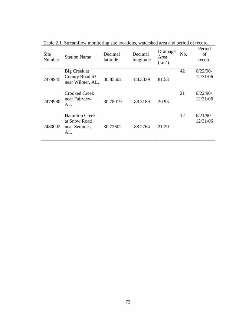
73
Table 2.1. Streamflow monitoring site locations, watershed area and period of record.
Site Number Station Name Decimal
latitude Decimal longitude
Drainage Area (km2)
No.
Period of
record
2479945
Big Creek at County Road 63 near Wilmer, AL.
30.85602 -88.3339 81.53
42 6/22/90- 12/31/06
2479980
Crooked Creek near Fairview, AL.
30.78019 -88.3189 20.93
21 6/22/90-12/31/06
2480002
Hamilton Creek at Snow Road near Semmes, AL.
30.72602 -88.2764 21.29
12 6/21/90-12/31/06

74
Table 2.2. Land use categories for Loading Simulation Program C++ classifications and watershed area of the Converse Watershed based upon 1992 multi-resolution land cover data. Land Use 1992 MRLC
land cover class
Base Cumulative watershed area (km2)
Percent of watershed
Future Watershed area (km2)
Percent of watershed
Urban 21+22+23+33 * 7.7 2.9%
59.7 22.2%
Barren 31 0.01 0.0% 0.01 0.0% Forest 41 + 42 + 43 165.6 61.6% 113.6 42.3% Pasture 81 + 85 45.3 16.9% 45.3 16.9% Cropland 82 32.9 12.2% 32.9 12.2% Wetlands 91 + 92 4.8 1.8% 4.8 1.8% Water 11 12.5 4.7% 12.5 4.7% Total 268.8 268.8 * Percent impervious designations follow Shen et al., 2005 (Low intensity residential (Class 21) = 12%; High intensity residential (Class 22) = 65%; Commercial/Industrial/Transportation (Class 23) = 85%; Transitional from one land use to another (Class 33) = 10%).

75
Table 2.3. Parameters for Loading Simulation Program C++ (LSPC) hydrologic calibration, suggested range of values and final calibration values for the Converse Watershed LSPC model. Parameter Description Result Range of
Values (units)
Final Values
AGWETP Fraction of evapotranspiration (ET) from active groundwater
An increases allows for more ET from wetlands
0.0 - 0.70 (none)
0.10 - 0.30
AGWRC Base groundwater recession
An increase flattens the base recession
0.850 - 0.999 (none)
0.991 - 0.998
BASETP Fraction of remaining ET from baseflow
An increase increases the difference between baseflow for different seasons
0.00 - 0.20 (none)
0.00 - 0.15
CEPSC Interception storage capacity
An increase allows for more interception
0.01 – 0.40 (inches)
0.01 - 0.15*
DEEPFR Fraction of groundwater inflow which is lost from the system to deep recharge
An increase reduces the streamflow
0.0 - 0.5 (none)
0.0 - 0.34
INFEXP Infiltration exponent
Regulates how lower zone storage affects infiltration rate
1.0 - 3.0 1.5 - 2.0
INFILD Ratio of maximum to mean infiltration capacity
Maximum infiltration is INFILD * input infiltration
1.0 - 3.0 2.0
INFILT Index to infiltration capacity
An increase results in a shift of drainage from surface runoff to baseflow
0.001 - 0.50 (inches hr -1)
0.01 - 0.45
INTFW Interflow inflow parameter
An increase decreases runoff by shifting surface runoff to
1.0 – 10.0 (none)
0.5 - 5.0

76
Parameter Description Result Range of Values (units)
Final Values
interflow
IRC Interflow recession parameter
An increase flattens recession and decreases peak flow
0.3 - 0.85 (none)
0.3 - 0.6
KVARY Variable groundwater recession
An increase causes groundwater to have a faster recession during wet periods
0.0 - 5.0 (inches-1)
0.0 - 0.5
LZETP Lower zone ET parameter – an index to deep rooted vegetation
An increase decreases surface runoff by increasing simulated ET
Maximum value ranges from 0.1 - 0.9 (none)
0.001 - 0.70*
LZSN Lower zone nominal soil moisture storage
An increase decreases flow by providing more opportunity for evapotranspiration
2.0 – 15.0 (inches)
7.0 - 9.0
NSUR Manning’s n for overland flow
An increase decreases velocity
0.1 - 0.5 (none)
0.12 - 0.35
UZSN Upper zone nominal soil moisture storage
Accounts for near surface water retention
0.05 - 2.0 (inches)
0.1 - 1.5*
* monthly values were used Range of recommended values from USEPA (2000).
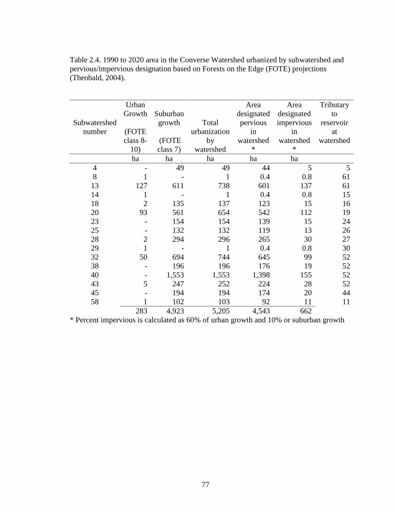
77
Table 2.4. 1990 to 2020 area in the Converse Watershed urbanized by subwatershed and pervious/impervious designation based on Forests on the Edge (FOTE) projections (Theobald, 2004).
Subwatershed number
Urban Growth
(FOTE class 8-
10)
Suburban growth
(FOTE class 7)
Total urbanization
by watershed
Area designated pervious
in watershed
*
Area designated impervious
in watershed
*
Tributary to
reservoir at
watershed
ha ha ha ha ha 4 - 49 49 44 5 5 8 1 - 1 0.4 0.8 61 13 127 611 738 601 137 61 14 1 - 1 0.4 0.8 15 18 2 135 137 123 15 16 20 93 561 654 542 112 19 23 - 154 154 139 15 24 25 - 132 132 119 13 26 28 2 294 296 265 30 27 29 1 - 1 0.4 0.8 30 32 50 694 744 645 99 52 38 - 196 196 176 19 52 40 - 1,553 1,553 1,398 155 52 43 5 247 252 224 28 52 45 - 194 194 174 20 44 58 1 102 103 92 11 11
283 4,923 5,205 4,543 662 * Percent impervious is calculated as 60% of urban growth and 10% or suburban growth

78
Table 2.5. Calibration (1991-2000) and validation (2001-2005) results for monthly total flow, direct runoff and baseflow at Big Creek, Hamilton Creek and Crooked creeks, Mobile County, Alabama. Statistics presented include the coefficient of determination (R2), Nash-Sutcliffe efficiency (NSE), ratio of the root mean square error to the standard deviation of measured data (RSR) and percent bias (PBIAS). R2 NSE RSR PBIAS Recommended criteria
> 0.5 <= 0.7 ± 25%
Big Creek Total flow 1991-2000 0.75 0.71 0.54 13.9 2001-2005 0.69 0.59 0.64 3.1 Direct runoff 1991-2000 0.65 0.52 0.69 35.8 2001-2005 0.70 0.45 0.74 16.2 Baseflow 1991-2000 0.84 0.83 0.41 0.6 2001-2005 0.63 0.61 0.62 -4.2
Hamilton Creek Total flow 1991-2000 0.67 0.60 0.63 14.5 2001-2005 0.72 0.69 0.56 2.5 Direct runoff 1991-2000 0.62 0.56 0.66 33.1 2001-2005 0.81 0.63 0.61 -4.7 Baseflow 1991-2000 0.71 0.63 0.61 7.2 2001-2005 0.67 0.62 0.62 4.7
Crooked Creek Total flow 1991-2000 0.71 0.67 0.57 6.6 2001-2005 0.70 0.61 0.62 -1.3 Direct runoff 1991-2000 0.72 0.57 0.66 29.6 2001-2005 0.73 0.52 0.69 19.2 Baseflow 1991-2000 0.67 0.64 0.60 -6.2 2001-2005 0.66 0.54 0.68 -10.4

79
Table 2.6. Annual total precipitation, simulated streamflow and observed streamflow (cm) for the base simulation. Simulated and observed streamflow converted from ft3 yr-1 to cm yr-1 [(ft3/yr) x (1 ac / 43,559 ft2) x (12 in / 1ft) x (1/watershed area in acres)]. Precipitation Big Creek Crooked Creek Hamilton Creek Year cm simulated observed simulated observed simulated observed 1991 207 3,998 5,370 1,118 1,227 1,245 1,425 1992 179 3,256 3,553 945 841 1,143 1,125 1993 153 3,078 4,209 719 973 1,133 1,219 1994 139 2,129 2,606 757 688 874 980 1995 204 4,036 4,161 1,374 1,156 1,346 1,532 1996 170 3,012 3,922 846 955 1,148 1,328 1997 178 3,246 4,026 1,120 1,402 1,130 1,671 1998 220 5,039 5,017 1,313 1,598 1,661 2,093 1999 129 2,029 2,070 937 925 930 1,034 2000 116 1,204 1,097 526 572 638 747 Mean 3,103 3,603 966 1,034 1,125 1,315 % difference
-13.9% ‘good’
-6.6% ‘very good’
-14.5% ‘good’
2001 139 2,111 1,656 523 589 848 709 2002 184 2,479 2,451 803 765 927 831 2003 180 4,056 4,897 986 932 1,323 1,278 2004 193 3,917 3,952 904 922 1,316 1,450 2005 188 4,343 4,483 1,176 1,130 1,468 1,775 Mean 3,381 3,488 878 868 1,176 1,209 % difference
-3.1% ‘very good’
1.2% ‘very good’
-2.7% ‘very good’
* streamflow performance ratings from Donigian (2002).

80
Table 2.7. Water quality parameters for TN, TP and TOC accumulation, storage, removal, interflow concentration and groundwater concentration by land use for the Converse Watershed model.
Land Use
Accumulation rate
Max surface storage
Runoff to remove 90% of stored
parameter
Interflow concentration
Groundwater concentration
acqop sqolim wsqop ioqc aoqc kg ha-1 day-1 kg ha-1 cm hr-1 mg L-1 mg L-1 TN Barren 0.08 c 0.39 c 2.0 c 0.05 c 0.05 c Crop 0.09 c 0.18 c 2.5 c 0.50 c 0.50 c Forest 0.01 c 0.02 c 3.3 c 0.50 f, l 0.50 f, l Pasture 0.22 c 0.56 c 2.0 c 0.80 c 0.50 c Urban 0.67 c 1.34 c 2.0 c 2.00 k 2.00 k Wetlands 0.06 c 0.11 c 3.3 c 0.50 i 0.50 i Urban impervious 0.34 c 0.67 c 1.3 c 2.00 k 2.00 k TP Barren 0.004 c, l 0.009 c 2.3 0.001 c, l 0.001 c, l Crop 0.008 c, e, l 0.016 c 2.3 0.100 c, l, k 0.030 c, l, k Forest 0.019 c, l 0.038 b, c, d 2.3 0.040 c, f, l 0.005 c, f, l Pasture 0.008 c, e, l 0.016 c 2.3 0.040 c, k, l 0.010 c, k, l Urban 0.009 c, l 0.018 c 2.3 0.060 c, k, l 0.030 c, k, l Wetlands 0.004 c, l 0.009 c 2.3 0.020 c, l 0.010 c, l Urban impervious 0.022 c, l 0.045 c 2.3 0.060 c, k, l 0.030 c, k, l TOC Barren 1.68 g 3.29 h 4.3 1.20 a, k 1.10 a, k Crop 2.13 g 2.40 h 4.3 5.90 a, k 2.90 a, k Forest 2.24 g 7.59 h 4.3 6.00 a, k 4.80 a, k Pasture 2.13 g 3.39 h 4.3 5.90 a, k 2.90 a, k Urban 1.18 g 14.39 h 4.3 1.30 a, k 1.28 a, k Wetlands 5.49 g j 34.98 h 4.3 6.20 a, k 1.10 a, k Urban impervious 1.18 g 3.29 h 4.3 1.20 a, k 1.28 a, k
a. Aelion et al., 1997 b. Alban, 1982 c. Childers, 2009 d. Furch, 1997 e. Macdonald and Bennett, 2009 f. Mulholland, 1992 g. Peters et al., 2007
h. Pouyat et al., 2006 i. Raghunthan et al., 2001 j. Reddy et al., 1993 k. Robinson et al., 2003 l. USEPA, 2009

81
Table 2.8. Loading Simulation Program C++ (simulated) and loadest (estimated) monthly load calibration (1991-2000) and validation (2001-2005) statistics for TN, TP and TOC at Big, Hamilton, and Crooked creeks, Mobile County, Alabama. n represents the number of samples utilized in loadest program linear regression. NSE RSR PBIAS Recommended criteria
> 0.5 <= 0.7 ± 25%
Big Creek TN (n = 70) 1991-2000 0.54 0.68 25 VG 2001-2005 0.61 0.62 7 VG TP (n = 69) 1991-2000 0.55 0.67 22 VG 2001-2005 0.27 0.85 6 VG TOC (n = 34) 1991-2000 0.50 0.71 37 G 2001-2005 0.59 0.65 26 G
Hamilton Creek TN (n = 70) 1991-2000 0.35 0.80 29 G 2001-2005 0.44 0.75 18 VG TP (n = 69) 1991-2000 0.39 0.78 45 S 2001-2005 0.57 0.65 32 G TOC (n = 35) 1991-2000 0.55 0.67 7 VG 2001-2005 0.33 0.82 -20 VG
Crooked Creek TN (n = 70) 1991-2000 0.73 0.51 11 VG 2001-2005 0.55 0.67 -1 VG TP (n = 69) 1991-2000 0.41 0.77 48 S 2001-2005 0.39 0.78 22 VG TOC (n = 36) 1991-2000 0.71 0.54 7 VG 2001-2005 0.62 0.61 -14 VG * PBIAS calibration quality results for N and P < ± 25 (very good), ± 25 - ± 40 (good) (Moriasi et al., 2007)

82
Table 2.9. Total nutrient load and median nutrient concentration to Converse Reservoir for base and future land use simulations, 1991 to 2005 TN TP TOC Total load (kg) Base 1,554,000 65,000 13,193,000 Future 3,252,000 105,000 16,557,000 % change 109% increase 62% increase 26% increase Minimum monthly load (kg mo-1) Base 1,970 43 15,203 Future 3,432 80 13,041 % change 74% increase 86% increase 14% decrease Median monthly load (kg mo-1) Base 6,367 206 49,013 Future 14,182 420 68,866 % change 123% increase 104% increase 41% increase Maximum monthly load (kg mo-1) Base 32,966 1,993 338,928 Future 65,245 2,485 395,220 % change 98% increase 25% increase 17% increase Concentration (mg L-1) Base 0.52 0.010 3.97 Future 0.82 0.017 3.34 % change 59% increase 66% increase 16% decrease

83
Table 2.10 Total simulated TOC flux (kg ha-1 yr-1
Year
) to Converse Reservoir by year for base and future scenarios, 1991 to 2005.
Base Future 1991 40.2 50.1 1992 32.6 42.0 1993 29.9 36.9 1994 21.3 29.0 1995 43.9 54.6 1996 31.1 38.6 1997 32.8 43.7 1998 52.8 59.0 1999 22.0 29.7 2000 12.7 17.8 2001 21.1 29.3 2002 26.6 37.5 2003 41.0 48.3 2004 40.1 50.5 2005 46.2 53.1

84
Table 2.11. Wilcoxon sign-ranked test of base and future monthly TOC loads (kg) to Converse Reservoir, 1991 to 2005. Bold numbers indicate a significant different (p < 0.05) between base and future monthly TOC loads. Month p-value January 0.0009 February 0.0054 March 0.0003 April 0.02 May 0.15 June 0.0001 July 0.0001 August 0.002 September 0.12 October 0.14 November 0.0006 December 0.0002

85
Figure 2.1. Monitoring locations, weather stations, and Mobile Area Water and Sewer
Systems (MAWSS) property in the Converse Watershed in southwestern Alabama. Watershed monitoring sites represent gauging and water quality monitoring locations.

86
0
50
100
150
200
250
1957
1960
1963
1966
1969
1972
1975
1978
1981
1984
1987
1990
1993
1996
1999
2002
2005
Year
Annu
al ra
infa
ll, c
m
Simulation period using measured precipitation
Figure 2.2. Annual rainfall (cm) from 1957 to 2005 at Mobile Regional Airport (Source: Mobile Regional Airport, reported by Earth Info, Inc)

87
Figure 2.3. Schematic of the Stanford Watershed Model adapted from Crawford and Linsley (1966). Circled numbers 1 to 5 denote the order in which water is removed to satisfy ET demand (TetraTech, 2008). AGWETP, active groundwater ET parameter; AGWRC, active groundwater recession; BASETP, baseflow ET parameter; CEPSC, interception storage capacity; DEEPFR, fraction to inactive groundwater; INFILT, infiltration parameter; INTFW, interflow parameter; IRC, interflow recession constant; LSUR, surface runoff length; LZETP, lower zone ET parameter; LZSN, lower zone storage capacity; NSUR, Manning’s surface roughness; SLSUR, surface slope; UZSN, upper zone storage capacity.

88
Figure 2.4. 1990 to 2020 urbanization scenario development for LSPC modeling of the Converse Watershed, Alabama. See text for description.
Primary Question: Which watersheds have the most urbanization between 1990 and 2020?
What is the housing density by watershed in 2020?
What is the housing density by watershed?
What is the change in
urban land in each
watershed between 1990
and 2020?
What is the change in
suburban land in each
watershed between 1990
and 2020?
Is the watershed owned by MAWSS?
Is Δ >= 2% of the total increase in suburban
land?
Is FOREST area by
watershed >= AREA Δ?
What is the land cover by watershed?
Question? Data Set
Scenario
FOTE 2020 Housing density
Class 0 - 10
FOTE 1990 Housing density
Class 0 - 10 LSPC
Watersheds
[2020 Class 7]–[1990 Class 7]
1. Δ watershed 1 2. Δ watershed 2 3. Δ watershed 3 . 62. Δ watershed
1992 NLCD
LSPC Watersheds
[2020 Class(8-10)]–[1990 Class(8-10)]
1. Δ watershed 1 2. Δ watershed 2 3. Δ watershed 3 . 62. Δ watershed
2020 housing density by watershed
Is the watershed owned by MAWSS?
Yes No
1992 land cover by watershed: water, crop,
pasture, barren, urban, wetland,
FOREST
Yes No
Omit No Yes
Add suburban and urban area to
determine total AREA Δ per
watershed
Yes
No Change all
FOREST land to urban land in
watershed in LSPC
Apply ‘AREA Δ’ by watershed to 1992 NLCD in LSPC (decrease forest - increase urban)
Pre-urbanizatio
1990 housing density by watershed
Post-urbanization
Omit
Omit
88

89
Figure 2.5. Forest to urban land conversion in the Converse Watershed from 1990 to 2020 by subwatershed. Subwatershed number, bold; acres changed from forest to urban in boxes. Each dot represents 20 acres changed from forest to urban land use within the subwatershed.

90
0
500
1000
1500
2000
2500
3000
3500
1/1/91 1/1/92 1/1/93 1/1/94 1/1/95 1/1/96 1/1/97 1/1/98 1/1/99 1/1/00
Time
Flow
(cfs
)0.001.002.003.004.005.006.007.008.009.0010.00
Tota
l Rai
nfal
l (in
)
Total Rainfall (in) Observed Flow Modeled Flow
0
200
400
600
800
1000
1200
1400
1600
1800
1/1/01 1/1/02 1/1/03 1/1/04 1/1/05
Time
Flow
(cfs
)
0.001.002.003.004.005.006.007.008.009.0010.00
Tota
l Rai
nfal
l (in
)
Total Rainfall (in) Observed Flow Modeled Flow
Figure 2.6. Observed and simulated streamflow at Big Creek during calibration (1991 to 2000) and validation (2001 to 2005). Daily precipitation from Mobile Regional Airport is shown.

91
0100200300400500600700800900
1000
1/1/1991 1/1/1992 1/1/1993 1/1/1994 1/1/1995 1/1/1996 1/1/1997 1/1/1998 1/1/1999 1/1/2000
Time
Flow
(cfs
)
0.001.002.003.004.005.006.007.008.009.0010.00
Tota
l Rai
nfal
l (in
)
Total Rainfall (in) Observed Flow Modeled Flow
0
50
100
150
200
250
300
350
400
1/1/2001 1/1/2002 1/1/2003 1/1/2004 1/1/2005
Time
Flow
(cfs
)
0.001.002.003.004.005.006.007.008.009.0010.00
Tota
l Rai
nfal
l (in
)
Total Rainfall (in) Observed Flow Modeled Flow
Figure 2.7. Observed and simulated streamflow at Crooked Creek during calibration (1991 to 2000) and validation (2001 to 2005). Daily precipitation from AWIS Semmes weather station is shown.

92
0
500
1000
1500
2000
2500
1/1/91 1/1/92 1/1/93 1/1/94 1/1/95 1/1/96 1/1/97 1/1/98 1/1/99 1/1/00
Time
Flow
(cfs
)
0.001.002.003.004.005.006.007.008.009.0010.00
Tota
l Rai
nfal
l (in
)
Total Rainfall (in) Observed Flow Modeled Flow
0
100
200
300
400
500
600
700
1/1/01 1/1/02 1/1/03 1/1/04 1/1/05
Time
Flow
(cfs
)
0.001.002.003.004.005.006.007.008.009.0010.00
Tota
l Rai
nfal
l (in
)
Total Rainfall (in) Observed Flow Modeled Flow
Figure 2.8. Observed and simulated streamflow at Hamilton Creek during calibration (1991 to 2000) and validation (2001 to 2005). Daily precipitation from Mobile Regional Airport is shown.

93
0
1000
2000
3000
4000
5000
6000
7000
8000
9000
10000
0 1000 2000 3000 4000 5000 6000 7000 8000 9000 10000 0
1000
2000
3000
4000
5000
6000
7000
0 1000 2000 3000 4000 5000 6000 7000 Monthly calibration Big Creek (R2 = 0.75)
Monthly validation Big Creek (R2 = 0.69)
y = 0.8402x + 121.15R2 = 0.7122
0
500
1000
1500
2000
2500
0 500 1000 1500 2000 2500
y = 0.7327x + 122R2 = 0.7042
0
200
400
600
800
1000
1200
1400
1600
1800
0 200 400 600 800 1000 1200 1400 1600 1800 Monthly calibration Crooked Creek (R2 = 0.71)
Monthly validation Crooked Creek (R2 = 0.70)
0
500
1000
1500
2000
2500
3000
3500
4000
0 500 1000 1500 2000 2500 3000 3500 4000 0
500
1000
1500
2000
2500
0 500 1000 1500 2000 2500 Monthly calibration Hamilton Creek (R2 = 0.67)
Monthly validation Hamilton Creek (R2 = 0.72)
Figure 2.9. Scatter plots of monthly streamflow during calibration (1991 to 2000) and validation (2001 to 2005) at Big, Crooked and Hamilton creeks in the Converse Watershed.

94
0
10,000
20,000
30,000
40,000
50,000
60,000
70,000
80,000
1991 1992 1993 1994 1995 1996 1997 1998 1999 2000 2001 2002 2003 2004 2005
Ann
ual T
N lo
ad (k
g/ye
ar)
LSPC LOADEST
Figure 2.10. Annual simulated (LSPC) and estimated (LOADEST) TN loads to Big Creek during calibration (1991 – 2000) and validation (2001 – 2005).

95
0
500
1000
1500
2000
2500
3000
1991 1992 1993 1994 1995 1996 1997 1998 1999 2000 2001 2002 2003 2004 2005
TP lo
ad (k
g/ye
ar)
LSPC LOADEST
Figure 2.11. Annual simulated (LSPC) and estimated (LOADEST) TP loads to Big Creek during calibration and validation.

96
0
100,000
200,000
300,000
400,000
500,000
600,000
700,000
1991 1992 1993 1994 1995 1996 1997 1998 1999 2000 2001 2002 2003 2004 2005
LSPC LOADEST
0
50,000
100,000
150,000
200,000
250,000
Jan-
91
Jul-9
1
Jan-
92
Jul-9
2
Jan-
93
Jul-9
3
Jan-
94
Jul-9
4
Jan-
95
Jul-9
5
Jan-
96
Jul-9
6
Jan-
97
Jul-9
7
Jan-
98
Jul-9
8
Jan-
99
Jul-9
9
Jan-
00
Jul-0
0
Jan-
01
Jul-0
1
Jan-
02
Jul-0
2
Jan-
03
Jul-0
3
Jan-
04
Jul-0
4
Jan-
05
Jul-0
5
TOC
load
(kg
per m
onth
)
LSPCLOADEST
Figure 2.12. Annual and monthly simulated and estimated TOC loads at Big Creek during calibration and validation.

97
0
50,000
100,000
150,000
200,000
250,000
1991 1992 1993 1994 1995 1996 1997 1998 1999 2000 2001 2002 2003 2004 2005
TOC
load
(kg/
year
)LSPC LOADEST
0
10,000
20,000
30,000
40,000
50,000
60,000
70,000
80,000
90,000
Jan-9
1Ju
l-91
Jan-9
2Ju
l-92
Jan-9
3Ju
l-93
Jan-9
4Ju
l-94
Jan-9
5Ju
l-95
Jan-9
6Ju
l-96
Jan-9
7Ju
l-97
Jan-9
8Ju
l-98
Jan-9
9Ju
l-99
Jan-0
0Ju
l-00
Jan-0
1Ju
l-01
Jan-0
2Ju
l-02
Jan-0
3Ju
l-03
Jan-0
4Ju
l-04
Jan-0
5Ju
l-05
TOC
load
(kg
per m
onth
)
LSPCLOADEST
Figure 2.13. Annual and monthly simulated and estimated TOC loads at Hamilton Creek during calibration and validation.

98
0
20,000
40,000
60,000
80,000
100,000
120,000
140,000
160,000
180,000
1991 1992 1993 1994 1995 1996 1997 1998 1999 2000 2001 2002 2003 2004 2005
TOC
load
(kg/
year
)
LSPC LOADEST
0
10,000
20,000
30,000
40,000
50,000
60,000
Jan-9
1Ju
l-91
Jan-9
2Ju
l-92
Jan-9
3Ju
l-93
Jan-9
4Ju
l-94
Jan-9
5Ju
l-95
Jan-9
6Ju
l-96
Jan-9
7Ju
l-97
Jan-9
8Ju
l-98
Jan-9
9Ju
l-99
Jan-0
0Ju
l-00
Jan-0
1Ju
l-01
Jan-0
2Ju
l-02
Jan-0
3Ju
l-03
Jan-0
4Ju
l-04
Jan-0
5Ju
l-05
TOC
load
(kg
per m
onth
)
LSPCLOADEST
Figure 2.14. Annual and monthly simulated and estimated TOC loads at Crooked Creek during calibration and validation.

99
0.00
10.00
20.00
30.00
40.00
50.00
60.00
70.00
1991 1992 1993 1994 1995 1996 1997 1998 1999 2000 2001 2002 2003 2004 2005
Tota
l str
eam
flow
(hm
mon
th-1
)
BaseFuture
Figure 2.15. Simulated total monthly base and future streamflow to Converse Reservoir, 1991 to 2005.

100
0
20000
40000
60000
Mon
thly
tota
l TN
load
(kg)
A.
0
500
1000
1500
2000
Mon
thly
tota
l TP
load
(kg)
B.
0
100000
200000
300000
400000
Mon
thly
tota
l TO
C lo
ad (k
g)
C. Figure 2.16. Monthly total TN (A), TP (B), and TOC (C) load (kg) to Converse Reservoir for base and future scenarios, 1991 to 2005. Symbols represent the smallest monthly load, lower quartile, median, upper quartile and largest monthly load.

101
1 2 3 4 5 6 7 8 9 10 11 12
0.0
0.1
0.2
0.3
0.4
0.5
Incr
ease
in T
N c
once
ntra
tion
(mg
L-1)
1 2 3 4 5 6 7 8 9 10 11 12
0.000
0.002
0.004
0.006
0.008
0.010
Incr
ease
in T
P c
once
ntra
tions
(m
g L-1
)
1 2 3 4 5 6 7 8 9 10 11 12-0.5
0.0
0.5
1.0
1.5
Incr
ease
in T
OC
con
cent
ratio
n (m
g L-1
)
Month Figure 2.17. Increase in estimated monthly TN, TP and TOC reservoir concentrations from allochthonous sources between base and future scenarios. Symbols represent the smallest monthly load, lower quartile, median, upper quartile and largest monthly load.

102
Chapter 3. Simulating the impact of urbanization on water quality of a public water supply reservoir, southern Alabama, USA.
3.1 Abstract Watershed model streamflow and water quality results were used in
Environmental Fluid Dynamics Code (EFDC) reservoir model to evaluate the difference
between pre- and post-urbanization concentrations of total nitrogen (TN), total
phosphorus (TP), total organic carbon (TOC) and chlorophyll a in raw water to be treated
for potable use. Source water TOC is especially important in Converse Reservoir due to
the potential for TOC to react with chlorine during the disinfection process and produce
carcinogenic disinfection byproducts (DBPs) regulated under the Safe Drinking Water
Act. Converse Reservoir simulation results based upon actual atmospheric conditions
from 1992 to mid-2005 were evaluated. EFDC calibration and validation performance
ratings for TN, TP, TOC and chlorophyll a ranged from ‘satisfactory’ to ‘very good’.
Median future TN, TP, TOC and chlorophyll a concentrations were higher than base
concentrations (p<0.05) during each month. Urbanization was found to increase total
median TN and TP concentrations by 55% and 67%, respectively. Predicted future
median TOC concentration was 1.1 mg L-1 (41%) higher than base TOC concentration at
the source water intake. Median TOC concentration increased by 0.02 mg L-1 km-2
following urbanization. The percent TOC change per area urbanized (%Δ / areaΔ) was
0.8 % per km2 urbanized area indicating that each km2 converted from forest to urban
land use increased TOC concentrations by 0.8%.

103
The highest simulated monthly median base and future TOC concentration
occurred in June whereas the highest measured median TOC concentration occurred in
July. Simulated and measured TOC concentrations reflect algae growth as chlorophyll a
accounted for most of the variance in TOC concentration between May and November
(R2 = 0.40 to 0.92). Tributary loading in March and April significantly influenced intake
TOC. Additional drinking water treatment beyond current practices is necessary when
raw water TOC concentration exceeds 2.7 mg L-1
3.2 Introduction
between May and October due to
distribution system temperature. Following simulated urbanization, TOC concentrations
at the source water intake between May and October increased by 33 to 49%. Monthly
results showed the largest increase in median TOC concentrations in August to October
(49%) due, in part, to the relatively low median base TOC concentrations in August to
October. Prior to urbanization, additional water treatment was necessary on 47% of the
days between May and October. Additional drinking water treatment was continuously
necessary between May and October following simulated urbanization.
Forested watersheds provide essential ecosystem services such as the provision of
high quality water. As watershed land becomes increasingly urbanized, the valuable
filtration services once provided by the forested catchments are lost. Drinking water
treatment authorities in locations such as Boston, MA, Portland, OR, and New York City
recognize the water quality benefits from forested catchments and actively purchase
natural land in supplying watersheds. An improvement in turbidity of 30% saved
$90,000 to $553,000 per year for drinking water treatment in the Neuse Basin of North
Carolina (Elsin et al., 2010). An analysis of 27 US water suppliers concluded a reduction
from 60% to 10% forest land increased drinking water treatment costs by 211% (Postel

104
and Thompson, 2010). The progressive loss of forest ecosystem services risks harm to
human health through lowered drinking water quality, as well as increased drinking water
treatment cost (Postel and Thompson, 2005).
One water quality variable of particular interest to water providers is total organic
carbon (TOC) because of disinfection byproduct (DBP) formation. Source water total
organic carbon (TOC) is a good indicator of the amount of DBP that may form as a result
of chemical disinfection (Singer and Chang, 1989). TOC reacts with chlorine during the
disinfection phase of water treatment to form DBPs. Several DBPs have been identified
by the US EPA as probable human carcinogens (USEPA, 2005b). Evidence is
insufficient to support a causal relationship between chlorinated drinking water and
cancer. However, US EPA concluded that epidemiology studies support a potential
association between exposure to chlorinated drinking water and bladder cancer leading to
the introduction of the Stage 2 DBP rule. The American Cancer Society (ACS) estimated
that there will be about 70,530 new cases of bladder cancer diagnosed in the United
States in 2010 (ACS, 2010). Approximately 2,260 drinking water treatment plants
nationwide are estimated to make treatment technology changes to comply with the Stage
2 DBP rule (USEPA, 2005b). An alternate method to mitigate DBP formation is the
management of watershed land use to reduce source water TOC (Walker, 1983; Canale et
al., 1997).
While water providers are struggling to maintain low source water TOC
concentrations and minimize DBP formation potential, source water catchments in the
southeastern US are undergoing rapid urbanization (Wear and Greis, 2002). The impact
of forest to urban land conversion on lotic TOC concentrations varies, however literature

105
reports elevated TN and TP concentrations in urban streams (Walsh et al., 2005).
Elevated nutrient concentrations can support increased algae growth thereby increasing
overall TOC in reservoirs regardless of the allochthonous contribution.
This research evaluates how simulated urbanization alters reservoir TOC
concentrations in a water supply reservoir, Converse Reservoir, Alabama. Converse
Reservoir supplies the drinking water for the City of Mobile, Alabama and surrounding
areas through the Mobile Area Water and Sewer Systems (MAWSS). MAWSS is one of
the >2,000 water treatment facilities nationally making changes to comply with the Stage
2 DBP rule. It was hypothesized that forest to urban land conversion in the Converse
Reservoir watershed may lead to increased reservoir eutrophication and challenges due to
elevated TOC concentrations and DBP formation.
Rapid urbanization is occurring in Converse Watershed, on the urban fringe of
Mobile, Alabama. Local, regional and national urbanization projections concur that the
Converse Watershed will likely undergo significant urbanization in the coming decades
(Wear and Greis, 2002; MMPO, 2005; Stein et al., 2005). Mobile source water TOC
concentrations may increase as urbanization occurs within the watershed. Mobile water
treatment officials evaluated alternate treatment strategies to comply with the Stage 2
DBP rule and found that raw water TOC >2.7 mg L-1 leads to elevated DBP in the
Mobile distribution system.
To evaluate the impact of forest to urban land conversion on reservoir water
quality paired watershed (Loading Simulation Program C++) and reservoir
(Envrionmental Fluid Dynamics Code) models were used. Daily nutrient concentrations
and streamflow from watershed simulations were utilized as input data to estimate the

106
effects on TOC concentrations within Converse Reservoir, AL under base and future land
use. TOC simulation results are vital because they lead to an understanding of effective
watershed and reservoir management to minimize source water TOC concentrations.
Overall (1992 to 2005) and monthly median TOC concentrations at a source water intake
from base and future scenarios were compared.
3.3 Objectives The objectives of this study were to 1) utilize paired watershed and reservoir
models to test the hypothesis that watershed nutrient loads during future scenarios will
lead to increased TOC concentrations and algae growth at the source water intake when
compared with base scenarios, 2) evaluate the influence of anticipated urbanization in
terms of the daily change in source water TOC concentrations and DBP formation
potential, 3) evaluate the influence of catchment urbanization on monthly median TOC
concentrations and algae growth at a source water intake.
3.4 Study Area Converse Reservoir was formed in 1952 by impoundment of Big Creek in Mobile
County, Alabama with a 37 meter high earthen dam. The reservoir is located ~6 km from
the Alabama-Mississippi border. Converse Reservoir, also referred to as Big Creek Lake,
supplies the majority of drinking water for the City of Mobile through the Mobile Area
Water and Wastewater Service (MAWWS). A 267 km2 watershed in the Southern Pine
Plains and Hills ecoregion of Alabama drains to the reservoir (Griffith et al., 2001). The
Converse Watershed is situated within the larger 2,797 km2 Escatawpa hydrologic
cataloging unit (HUC 03170008) (Seaber et al., 1994). The physical characteristics of the
reservoir, summarized by Journey and Gill (2001) include: volume (64,100,000 m3),
surface area (14.6 km2), mean depth (4.4 m), and maximum depth (15.2 m). Mean depth

107
was calculated by dividing volume by surface area. Centerline length of Converse
Reservoir mainstem is 12.1 km, with an average reservoir width of 1 km. Estimated
shoreline is 81 km, with a shoreline development index of 6.0, characteristic of elongate
reservoirs (Lind, 1985). Converse Reservoir has two main branches, Big Creek, which
becomes the mainstem of the reservoir, and Hamilton Creek. The drinking water intake is
on Hamilton Creek 4.8 km from the mainstem of the reservoir.
A preliminary evaluation was conducted to confirm the ability of the EFDC
model to simulate how changes in upstream nutrient loads influence water quality at the
drinking water intake. Average water surface elevation at the spillway is 33.53 m above
mean sea level (msl). Maximum watershed elevation is 59.4 m above msl. Figure 2.1
depicts the watershed location within Alabama, along with weather stations and water
quality monitoring locations in the Converse Watershed.
Converse Reservoir receives inflow from seven major tributaries, as well as
groundwater inflow. A firm-yield analysis of Converse Reservoir estimated ~5% of the
total volume is from groundwater (Carlson and Archfield, 2008). Streamflow from the 3
major tributaries (Big, Crooked and Hamilton creeks) has been monitored by USGS
gauging stations since 1990. Big Creek contributes one-half of the gauged inflow to
Converse Reservoir and Hamilton Creek contributes ~20 percent (Journey et al., 1995).
The Miocene-Pliocene aquifer ranges in thickness from 30.5 to 1,036-m thick in
Mobile and Baldwin counties and is ~305 m-thick beneath the Converse Watershed. The
aquifer supplies baseflow to streams (Mooty, 1988). The 61 m-thick Citronelle geologic
unit overlies the Miocene series. The sand and gravel beds of the Citronelle and upper
Miocene are hydraulically connected to the land surface; therefore, groundwater is

108
susceptible to surface contamination (Gillett et al., 2000). In the deeper portions of the
aquifer, clayey sediments can cause it to be semiconfined, which reduces the vertical
infiltration of water (Journey and Gill, 2001). The sediments in Converse watershed are
somewhat resistant to weathering and contribute relatively little to surface water
chemistry. Water pH tends to be more acidic and have low specific conductance
(Journey and Gill, 2001).
Concerns about the quality of Converse Reservoir as a supply source for drinking
water led to various scientific investigations (Journey et al., 1995; ADEM, 1996; Bayne,
et al., 1998; Journey et al., 2001; ADEM, 2003; Gill et al., 2005). Tributary and reservoir
water quality data have been collected by the United States Geological Survey (USGS),
Auburn University (AU) and MAWSS under various sampling programs and intervals
from 1990 to 2005 as described in Appendix A. Algae growth potential tests conducted
in 1997, 2001 and 2006 indicate P generally limits algae growth in Converse Reservoir
(Bayne et al., 1998; ADEM, 2007). Converse has a history of extended anoxic periods,
which may contribute to internal nutrient loading (Journey and Gill, 2001).
Precipitation near the City of Mobile is some of the highest in the US, with a 48-y
(1957-2005) median monthly precipitation of 12.40 cm (1953 – 2005). Modeling in this
project relies on historic rainfall data, so it is important that the periods of model
calibration and validation include representative wet and dry conditions (Figure 2.2).
Based upon Soil Survey Geographic (SSURGO) data, the Troup soil series covers
37% of the watershed and Troup-Benndale and Troup-Heidel cover another 14 and 6%,
respectively (USDA, 2004). Heidel and Bama Soil Series cover 13 and 67%,
respectively. All other soil series each (15 total) cover <5% of the watershed area each.

109
Watershed soils are generally acidic, low in natural fertility and organic matter content
and composed of fine sand or loamy find sand. These soils are considered well to
moderately well drained. They are classified as soil hydrologic group A and B soils,
having low to moderately low runoff potential and <20% clay (USDA, 2007).
Within the Converse Watershed there are wetlands, forests, dairy farms, plant
nurseries, pecan groves and residential areas that utilize septic tanks for sewage disposal.
Between 1990 and 2005 there were 2 known facilities with National Pollution Discharge
Elimination System (NPDES) permits in the watershed. Both are associated with
construction, one draining to Collins Creek (AL0064904) and the other discharging to
groundwater near Hamilton Creek (AL0064530). MAWSS owns roughly 36.4 km2
surrounding the reservoir (approximately 11.5% of the total watershed area), which is
managed for timber production by MAWSS.
The eastern watershed boundary extends to within 500 m of Mobile, Alabama,
city limits. New road construction is expected along with increased urbanization. The
Mobile Metropolitan Planning Organization (MMPO) Transportation Plan (2000 to 2030)
depicts a new freeway loop bisecting the eastern portion of the watershed (MMPO,
2005). Relocation of Highway 98 to the north within the watershed in 2007 generated
litigation due to failed Alabama Department of Transportation (ALDOT) erosion control
(ALDOT, 2010). Future forecasts of urbanization in the Southeastern US reported by the
Southern Forest Resource Assessment (Wear and Greis, 2002) indicated that major
urbanized centers will be concentrated in 3 large areas. One of these was the Gulf Coast
centered on Mobile Bay, which encompasses the Converse Watershed. The Forests on
the Edge project (FOTE, Stein et al., 2005) evaluated urbanization at a national scale and

110
depicted increased population and urban housing densities within the Converse
Watershed every 10 y between 1990 and 2030. Local, regional and national urbanization
studies described above concur that the Converse Watershed will likely experience
significant urbanization in the coming decades.
3.5 Methods EFDC simulations were first conducted using uncorrected inflows from LSPC and
water surface elevation was analyzed. Next, 4 s time-step simulations were conducted
using constant outflows and corrected water surface elevation was recorded daily. After
hydrodynamic routines were executed water quality simulations were conducted.
3.5.1 EFDC Hydrodynamic Model The EFDC hydrodynamic model was developed at the Virginia Institute of
Marine Science beginning in 1988 (Hamrick, 1992). EFDC can be used to simulate both
hydrodymanics and water quality. The model has been applied in various locations,
including Chesapeake Bay estuarine system (Hamrick, 1994), the Neuse Estuary in North
Carolina (Wool et al., 2003) and the Florida Everglades (Moustafa and Hamrick, 2000).
It has been used in a wide range of environmental studies including simulations of
pollutant and pathogenic organism transport, simulation of power plant cooling water
discharges, simulation of oyster and crab larvae transport, and evaluation of dredging and
dredge spoil disposal alternatives (Tetra Tech, 2006a). It has evolved over the past
several decades to become one of the most technically defensible and widely used
reservoir models available (USEPA, 2010). EFDC utilizes FORTRAN 77 code and
requires a several text based input files to supply water elevation (pser.inp), stream
inflows (qser.inp), atmospheric conditions (aser.inp and wser.inp), and grid parameters.
Lake evaporation is internally computed using a latent heat transfer equation documented

111
in Hamrick and Mills (2000). The model creates output files that are viewed in the Water
Quality Analysis Simulation Program (WASP) post processor. The EFDC hydrodynamic
model provides the hydrologic basis for a number of other water quality models such as
Water Quality Analysis Simulation program (WASP5) (Ambrose, et. al., 1993) and the
multi-dimensional surface water model (CE-QUAL-ICM) (Cerco and Cole, 1995).
3.5.2 EFDC Water Quality Model EFDC water quality simulation requires several additional input files.
WQ3DWC.inp is the master water quality input file containing information about the
simulated water quality variables, the load input locations, and values for rates and model
parameters controlling simulation of water quality variables. WQPSL.inp is the file
containing daily loads for the streams draining to Converse Reservoir. Details regarding
model set-up and theoretical basis are provided in the EFDC User’s Manual (Tetra Tech,
2006a) and the EFDC Theory and Computation Manual (Tetra Tech, 2006b).
3.5.3 Scenarios Base 1992 MRLC land cover served as the base (pre-urbanization) scenario for
comparison with the future (2020) scenario. The 2020 scenario was generated from the
population-based housing density forecasts of the FOTE project (Stein et al., 2006). To
quantify the economic value of forest land for water quality, only forest to urban land
conversion was simulated in future scenarios. Between base and future simulations only
daily LSPC-derived streamflow and TN, TP and TOC loads to Converse Reservoir
changed. All other input files remained constant in base and future scenario simulation.
Base and future urbanization scenarios were compared with each other to estimate the
influence of forest to urban land conversion on reservoir water quality.

112
3.5.4 Simulation Period EFDC simulation occurred over two time periods between 1 July 1991 and 30
April 2005. A severe drought in 2000 caused MAWSS to decrease reservoir surface
elevation by nearly 3 m. Changes to water quality under average conditions were the
focus of this study and the year 2000 provides the divide between calibration and
validation, but was not simulated or included in analyses.
EFDC is run for 6 mo (Jul to Dec 1991 and Feb to Jul 2001) prior to results
comparison to minimize the influence of initial conditions such as reservoir constituent
concentrations on model simulation. A test of the influence of initial concentrations at
the source water intake indicated similar nutrient concentrations at the source water
intake regardless of initial concentrations after six months of simulation.
Time periods for calibration, validation and model scenarios are reported in Table
3.1. The calibration and validation years correspond with the years of the greatest
number of reservoir water quality measurements. Detailed calibration and validation
methods are provided in section 3.5.7.
3.5.5 Model Configuration
Orthogonal Reservoir Model Grid Generation Topographic maps were available which reflected the watershed prior to reservoir
creation in 1952. The maps were surveyed in 1941-1942 and produced by the USGS and
Army Corps of Engineers. Photographs of these maps were imported into ArcMap
Version 9.1 and georeferenced to 7.5-minute topographic maps from 1985-86 for the
reservoir.
Projected maps were utilized to digitize reservoir bathymetry. The normal water
level elevation was 33.53 m above msl and each contour line represents a change of 3.05

113
m in elevation. Five contour lines were digitized as the reservoir has a maximum depth
of ~ 15.24 m. The digitized polyline shapefiles were utilized to assign a depth in meters
to each grid cell described below.
VOGG: A Visual Orthogonal Grid Generation Tool for Hydrodynamic and Water
Quality Modeling was utilized to generate the grid required for reservoir modeling (Tetra
Tech, 2002). The steps to operate the VOGG tool include: (1) import reservoir water
boundary, (2) create control points, (3) generate grid, (4) delete unwanted cells and (5)
input water level and reservoir depth values for each grid cell. The resulting grid was
then used as the reference system for EFDC modeling. Eight control points were used to
create a 60 by 45 curvilinear grid array. Cells outside the reservoir boundary were
deleted leaving a total of 575 grid cells to simulate Converse Reservoir (Figure 3.1). The
mean cell width was 178 m (range: 139 – 208 m). The mean cell height was 186 m
(range: 96.5 – 390 m). The water level was determined from the measured water surface
elevation during the first day of simulation and fluctuated with each time step during
simulation. The bottom elevation of each cell was the elevation of the cell with respect to
MSL.
Atmospheric Data Hourly local climatological data available from the National Climactic Data
Center (NCDC) for the Mobile Regional Airport weather station for the monitoring
period were provided by EarthInfo, Inc (2006). EarthInfo, Inc. supplies NCDC
atmospheric data formatted for use by the meteorological data analysis and preparation
tool (MetAdapt) program. The EarthInfo files required by the MetAdapt program
included ‘summary of the day’, ‘hourly precipitation’ and ‘surface airways’ data.
MedAdapt was utilized in this study to format and prepare the necessary atmospheric

114
data for EFDC. Two atmospheric input files (aser.inp and wser.inp) were generated that
included hourly barometric pressure, air temperature, dewpoint temperature, rainfall,
solar radiation, and cloud cover, wind speed and wind direction. Atmospheric data files
used in this study were checked by plotting hourly pressure, temperature, humidity and
precipitation in Microsoft Excel to ensure that values fell within expected ranges. Hourly
pressure values for 3 July 1997 were unrealistically low and deemed anomalies, and were
modified to be the mean of the preceding and subsequent hourly values. One temperature
(-17.8º C) and several humidity values (1.04) were also modified to be the mean of
preceding and subsequent hourly values after detecting obvious anomalies. Extreme
precipitation values were confirmed by comparing with stormdata publications and
hurricanes. Following verification and necessary data infilling atmospheric data were
utilized as input in reservoir model simulation.
Reservoir inflows and outflows The input file which stores streamflow and outflow data (qser.inp) was created
using modeled LSPC streamflow. Inflows from all watersheds draining to Converse
Reservoir were apportioned to one of five inflows to Converse Reservoir. Table 3.2
describes the output watersheds that correspond with each inflowing stream. The five
simulated inflows to Converse Reservoir are Hamilton Creek, Crooked Creek, Big Creek,
Long Branch, and Boggy Branch. The two outflows were dam spillage and pumpage for
water treatment, taken from MAWSS records. Lake evaporation was internally
computed using a latent heat transfer equation documented in Hamrick and Mills (2000).
Dam seepage and groundwater interaction were not simulated by EFDC.

115
Simulation outflow correction Simulation using inflow from watershed models and measured spillway outflows
causes differences between the simulated and measured water surface elevation (WSE).
The watershed model urban scenario had significantly higher inflow than the base
scenario. Model simulations were first conducted without flow correction. Measured
and simulated daily WSE results at the dam spillway were plotted to determine if a
constant outflow was necessary to achieve similar modeled and measured WSE.
Constant outflow correction was selected rather than inflow adjustment as adjusting
inflows during simulation to make simulated WSE consistent with measured WSE would
alter the nutrient loads to the reservoir.
Adjustments were made only to spillway outflows to correct WSE. If WSE
decreased to the point of shallow cell drying, then measured spillway outflows were
adjusted or deleted. If WSE consistently increased, then a constant outflow was
estimated from the linear slope of WSE increase and removed as spillway outflow on a
daily basis to achieve relatively consistent measured and simulated water surface.
Tributary inputs The 11 daily input variables at each stream included: green algae, particulate and
dissolved C, particulate and dissolved organic P, orthophosphate, particulate and
dissolved organic N, nitrate+nitrite, ammonia and dissolved O2
Measured data were used to partition watershed model TN concentrations into
TON, nitrate and ammonium values based upon the following relationship; TN is the sum
(Table 3.3). Daily TN,
TP and TOC concentrations from the watershed model were partitioned into nutrient
fractions for the EFDC model based upon measured data for each stream as described
below.

116
of inorganic N [nitrate and ammonium] and organic N. Organic N was simulated in
either the dissolved or particulate form. TON was assumed to be ~20% particulate and
80% dissolved based upon the measured proportions of PON and DON in a limited
number of samples at Big (TON n=20; DON n=14), Crooked (TON n=21; DON n=21)
and Hamilton (TON n=20; DON n=17) creeks.
Dissolved and particulate organic P were partitioned based upon the following
relationship; TP = particulate organic P + dissolved organic P + orthophosphate.
Measured TP, dissolved P and orthophosphorus were used to calculate the percentage of
incoming simulated TP as dissolved organic, particulate organic and inorganic
(orthophosphate) at all 5 tributaries flowing into Converse Reservoir. Organic C was
simulated in particulate and dissolved forms. Measured TOC and DOC data were used to
partition the simulated TOC from the watershed model into dissolved and particulate
fractions.Daily values of 2 µg L-1 for green algae chlorophyll a were input. Measured
data are used to estimate mean monthly dissolved oxygen at each stream. Dissolved
oxygen concentrations were used to calculate daily values. Daily concentrations were
converted to daily loads and a program was used to reformat the daily loads into the
wqpsl.inp file used in simulation.
3.5.6 Calibration and validation Flows and nutrient loads derived from the LSPC watershed model of 2001 MRLC
land cover (Homer et al., 2004) were utilized during calibration and validation.
Calibration is the process of parameter adjustment to achieve similar measured and
simulated values. Validation is the use of an alternate data set to test the calibrated
model. Model validation is an extension of the calibration process. The purpose of
validation is to assure that the calibrated model performs properly under various

117
conditions which can affect model results and to demonstrate the ability to predict field
observations for periods of time separate from calibration.
The common and recommended calibration and validation methodology is to use
available measured data from one time period for calibration and available measured data
from another time period for validation, which is the method employed in this study
(Donigian, 2002). Model performance is evaluated through graphical comparisons and
statistical tests.
Reservoir calibration (2001 to 2003) and validation (1996 to 1999) time periods
were selected based upon monitoring data availability. Reservoir data near the source
water intake were most plentiful in 1997, 2002 and 2003. The calibration period includes
one year of below average precipitation (2001) and two years of above average
precipitation (2002 and 2003). The validation period also has one year of below average
precipitation (1999) and three years of above average precipitation (1996 to 1998).
Watershed model streamflow and loads from the 2001 MRLC land cover, which is
temporally closer to the calibration and validation time frames than the 1992 MRLC land
cover, were used. The amount of barren land (~0%), forest land (~60%) and pasture land
(~15%) and water (~5%) were similar in the 1992 and 2001 land cover datasets (Table
3.4). Percent urban and wetland area were larger in 2001 than 1992. Percent cropland
was less in 2001 (2.7%) than 1992 (12.2%). These differences in watershed land cover
between 1992 and 2001 likely had little influence on reservoir model calibration and
validation.
Water Surface Elevation Flow Correction A flow correction calculation was utilized during calibration and validation to
ensure that simulated WSE corresponded with measured water surface elevation. The

118
flow correction was calculated on a daily basis. To correct WSE, inflow adjustments
were applied to the most upstream tributary (Big Creek) and outflow adjustments were
applied at the spillway. The goal of flow correction was to achieve similar measured and
simulated lake levels to minimize the influence of variation in simulated hydrodynamics
and WSE on calibration and validation of water quality variables. Following flow
modifications, measured and predicted WSE were compared. WSE measured at midnight
of each day at the Converse dam spillway was compared with simulated WSE at
midnight (cell 23,7).
WSE flow correction was conducted for calibration and validation independently.
The correction flow was calculated daily using a mass-balance approach. The measured
volume change was computed daily (change in water level x reservoir area). The mass-
balance volume change was also computed daily using simulated inflows for all
tributaries, precipitation volume, spillway and drinking water outflows and estimated
evaporation. The difference between the measured volume change and the mass-balance
volume change provided an overall daily correction volume, which was converted to a
flow rate. A new streamflow input file (qser.inp) with corrected flows was created and
used during calibration. Corrected streamflow was used to generate a new corrected
daily loads file for calibration (wqpsl.inp).
Water Quality calibration and validation Once flows were adjusted such that simulated WSE corresponded with measured
WSE, chlorophyll-a, TN, TP and TOC, parameters were adjusted to achieve similar
simulated and measured water quality near the drinking water intake. Data collected by
USGS, Auburn University in Dr. David Bayne’s laboratory (Department of Fisheries and
Allied Aquacultures) and MAWSS were used in calibration.

119
During calibration a total of 17 profiles were collected for temperature and
dissolved oxygen (DO) at the reservoir monitoring station nearest the MAWSS drinking
water intake. During validation a total of 13 profiles were collected for temperature and
DO. Individual DO values were collected on 25 additional sampling days during
validation. Temperature data were collected using a YSI thermistor and DO was
collected using the membrane electrode method (APHA, 1995).
The total number of chlorophyll-a samples (µg L-1
TOC data (mg L-1) for calibration and validation were collected by AU, USGS
and MAWSS (Bayne et al., 1998; Journey and Gill, 2001). The total number of TOC
samples used in assessing calibration and validation was 38 and 143, respectively.
MAWSS and USGS samples are analyzed using method 5310-B (APHA, 1995). The 12
samples collected by AU in 1997 were analyzed using method 5310-C (APHA, 1995).
) for calibration and validation
at MAWSS drinking water intake were 17 and 21, respectively. Most chlorophyll-a
samples were analyzed using standard method 10200H, a high-performance liquid
chromatography method (APHA, 1995). The 1997 samples analyzed by AU utilized a
spectrophotometric method (Bayne et al., 1998).
TP samples (mg L-1) for calibration (n=18) and validation (n=23) were collected
and analyzed by USGS and AU using similar colorimetric methods. TN samples (mg L-
1
3.5.7 Data Analyses
) for calibration (n=18) and validation (n=24) were collected and analyzed by USGS and
AU using similar colorimetric methods.
Model calibration and validation statistics
Daily EFDC results were provided for each cell at 5 depths. A mean of the values
for each depth at the MAWSS source water intake (cell 34,18) was calculated. Absolute

120
mean error (AME), fractional AME and percent bias (PBIAS) performance ratings were
provided. PBIAS performance ratings (Moriasi et al, 2007) were published for monthly
mean values, but here were applied to daily grab samples as multiple monthly samples
for water quality were rarely collected. Moriasi et al. (2007) recommended the use of
graphs to evaluate calibration and validation quality where a continuous dataset was
unavailable. Time-series plots of simulated and measured water quality were developed
for visual comparison. Profile plots of measured and simulated temperature and DO in
the channel near the drinking water intake (cell 27,18) were also developed. Model
calibration and validation were deemed acceptable based upon time-series plots, as well
as comparison of AME and PBIAS performance ratings. All statistical data analyses are
conducted in S-PLUS 6.2 professional (Insightful Corporation, 2003).
Base and future scenario statistics Daily concentrations at the MAWSS source water intake for the simulated water
quality variables and urbanization scenarios were analyzed for normality using
histograms and quantile-quantile normal plots of residuals. If data were not normally
distributed, differences between scenarios were determined using nonparametric
comparison methods such as the Wilcoxon Sign-Ranked (WSR) test (Wilcoxon, 1945).
WSR was used to compare daily and monthly median base and future concentration
results.
The change in median TN, TP and TOC concentration and percent difference
between base and future scenarios were reported. Concentration change following
urbanization was reported in terms of land use change. The percent change per area
change (%Δ / areaΔ) metric was calculated as the percent difference between base and
future concentrations divided by the simulated change in forest to urban land (km2).

121
Time-series plots display differences between daily base and future TN, TP, TOC and
chlorophyll a concentrations.
Monthly median simulated and measured TOC concentrations were compared.
The percent difference in monthly median TOC between base and future scenarios was
reported. Monthly base and future scenario regression was performed using monthly
median chlorophyll a, monthly TOC load and both to predict TOC response. In
regression analyses, monthly median TOC concentration was the response variable and
monthly median chlorophyll a and monthly Hamilton Creek loads were independent
variables. Since data were not normally distributed, they were log10 transformed before
regression analyses.
TOC threshold for drinking water treatment Minimum TOC concentration at the source water intake was analyzed in terms of
drinking water treatment level. The finished water TOC concentration of 1.5 mg L-1 or
less minimizes the formation of DBP in MAWSS drinking water distribution system.
Between May and October, when water temperature is generally >26.7º C, raw water
TOC must be <2.7 mg L-1 to have a finished water TOC concentration of 1.5 mg L-1,
given the 45% TOC removal efficiency at MAWSS drinking water treatment plants.
Additional treatment is necessary when reservoir TOC concentrations were >2.7 mg L-1.
The number of days when reservoir TOC exceeded the 2.7 mg L-1 level between May and
October were reported. An exceedence probability plot of monthly median TOC
concentrations for base and future scenarios was generated.

122
3.6 Results and Discussion
3.6.1 Water surface elevation constant outflow correction A constant outflow correction was applied between 2001 and 2005 in the future
scenario. A constant outflow of -15.9 MGD was removed at the dam spillway from 2001
to 2005. Constant outflow correction was necessary because simulated water level rose
above measured water level. Simulated water level increased for several reasons. LSPC
streamflow was higher in future scenarios, so WSE increased in response to increased
simulated inflows. Additionally, deep percolation and dam seepage are not simulated in
the Converse Reservoir model. Carlson and Archfield (2008) reported that in their
simulated firm yield analysis of Converse Reservoir, water flowed into the aquifer
between 2002 and 2006. Between 2002 and 2006 the aquifer below Converse Reservoir
may have been recovering from its depletion during the 2000 drought year. The constant
outflow correction between 2001 and 2005 may have been making adjustments which
accounted for the lack of simulated deep percolation. Other reasons for an increase in
water level over time include possible overestimation of precipitation reaching the lake
surface and/or underestimation of lake evaporation or evapotranspiration from aquatic
plants.
In general, measured outflow at the spillway was used for all simulations.
Occasionally, the measured outflow did not correspond well with the simulated inflows
causing problems for simulation due to water level decline. This occurred most
frequently during the base scenario, where simulated inflows were less than post-
urbanization scenario inflows. The edited outflows corresponded with years of negative
annual mass balance (1993 and 1996 to 1999), where there was more outflow than inflow
or precipitation. At times, hurricanes or large storms caused large flows and model

123
instability. These large flows when they occurred were averaged over a number of days
to mitigate instabilities in model simulation water level.
3.6.2 Calibration and validation results
Mass balance correction for water surface elevation The total inflow and outflow correction volume is provided in Table 3.5. The
average daily outflow correction volume was similar during both calibration and
validation. The average measured spillway outflows during calibration and validation
were similar, 0.37 and 0.40 million m3
Time series plots of water surface elevation used during water quality calibration
and validation (Figure 3.2) show that measured and simulated water level corresponded
well. Mean simulated WSE during calibration was 0.03 m higher than mean measured
WSE (33.42 and 33.39 m, respectively). Mean simulated WSE during validation was
0.21 m higher than mean measured WSE (33.32 and 33.53, respectively).
, respectively. Average daily inflow correction
during validation (1996 to 1999) was more than twice the average daily inflow correction
during calibration (2001 to 2003). This difference may be due to differences in simulated
inflows; during validation the error in total inflow volume for the largest tributary (Big
Creek) total simulated streamflow was 8% less than observed streamflow. In contrast,
during calibration, the simulated streamflow was 8% more than observed streamflow.
Under-estimated streamflows during validation caused a need for a larger average daily
correction flow to achieve similar measured and simulated WSE. The larger correction
inflows from 1996 to 1999 than 2001 to 2003 may also reflect the absence of simulated
deep percolation during the aquifer recharge period of 2002 to 2006 (Carlson and
Archfiled, 2008) effectively causing a higher WSE than if the recharge had been included
in simulation during calibration (2001 to 2003).

124
Water quality calibration and validation results Results of simulated and observed mean, standard deviation, absolute mean error
(AME), fractional AME and percent bias (PBIAS) for calibration and validation are
provided in Table 3.6.
Temperature calibration and validation
During calibration, mean values for temperature profiles collected on 17 days for
observed and simulated data were 26.2 ºC and 27.0 ºC, respectively (Table 3.6; Figure
3.3). An AME of 1.0 indicates that, on average, the predicted temperature values were
within 1.0 º C of the observed values. The PBIAS of -3.1 % for temperature calibration
indicates ‘very good’ performance (Donigian, 2002). Fractional AME (or relative error)
is a normalized statistic and allows for comparison with other model applications.
Temperature fractional AME was 4%.
The mean values for temperature profiles collected on 35 days during validation
for observed and simulated data were 21.5 ºC and 21.3 ºC, respectively. The PBIAS of
1.7 for temperature validation indicated ‘very good’ performance (Donigian, 2002)
(Figure 3.3). Temperature and DO profiles of observed and simulated data during
calibration and validation indicate good model performance.
Dissolved oxygen calibration and validation
During calibration, the mean of all DO profiles for observed (6.3 mg L-1) and
simulated (6.1 mg L-1) data over 17 sampling days corresponded well. The predicted DO
values were within 0.86 mg L-1 of the observed values. PBIAS performance ratings for
DO were not provided by Moriasi et al. (2007) or Donigian (2002). However applying
performance ratings for temperature to dissolved oxygen, PBIAS calibration performance
for DO was ‘very good’ (3.6%). DO fractional AME was 0.14, similar to EFDC

125
modeling applications at Cape Fear River, NC (0.12 – 0.15), Charleston Harbor, SC (0.08
to 0.21), and Charles River, MA (0.07 – 0.21) (Tetra Tech, Inc, 2006b). The Converse
EFDC model predicted DO levels well and within ranges reported by other EFDC
applications.
During validation, mean observed and simulated DO concentrations were 8.0 mg
L-1 and 6.9 mg L-1, respectively. DO fractional AME of 0.16 was within the reported
range of other calibrated EFDC models of 0.04 to 0.40 (Tetra Tech Inc, 2006b).
Applying performance ratings for temperature to DO, PBIAS validation performance for
dissolved oxygen (13%) was ‘fair’.
Nutrient calibration and validation During calibration, TN, TP and TOC concentration performance ratings were
‘very good’ based upon PBIAS. On average, predicted TN values were within 0.1 mg L-1
of observed values. Mean of daily observed and predicted TP concentrations were 0.007
and 0.006 mg L-1, respectively. Mean daily observed and predicted TOC were 3.9 and
3.5 mg L-1, respectively. On average, predicted TOC values were within 0.8 mg L-1 of
observed TOC values. The calibrated EFDC model appears to slightly under-predict TP
and TOC. Figures 3.4, 3.5 and 3.6 provide calibration time series plots of simulated and
measured TN, TP and TOC, respectively. TN fractional AME was 0.26, which was
within the range reported for a calibrated model of St. Johns River (Tillman et al., 2004)
and other calibrated EFDC models (Tetra Tech, Inc, 2006b). TP fractional AME was
0.66, which was within the ranges reported for other calibrated reservoir models (Tetra
Tech, 2006). TOC fractional AME was 0.21, which is less than values reported for
Florida Bay (Cerco et al, 2002) and similar to St. Johns River (Tillman et al., 2004).

126
Nutrient and TOC calibration were similar to previous EFDC applications and ‘very
good’ based upon PBIAS performance ratings.
During validaiton, TN, TP and TOC concentration preformance ratings were
‘good’ to ‘very good’ based upon PBIAS. The mean observed and simulated TN
concentrations during validation were 0.38 and 0.47 mg L-1, respectively. Simulated TN
was higher than observed TN, with an AME indicating that predicted TN was within 0.11
mg L-1 of observed TN. Fractional AME for TN (0.29) was within the range of reported
values from other EFDC applications. TN validaiton performance rating based upon a
PBIAS of 25% was ‘good’ (Moriasi et al., 2007). Figure 3.4 shows simulated and
observed TN concentration during calibration and validation indicating good model
performance. While EFDC slightly overpredicted in-reservoir TN concentrations, it
slightly underpredicted TP concentrations. Mean observed and simulated TP
concentrations during validation were 0.015 and 0.010 mg L-1, respectively. The
fractional AME of 0.56 for TP validation was within reported values for other EFDC
applications (Tetra Tech, 2006). PBIAS for TP during validation was 40% indicating
‘good’ model performance. Observed (3.54 mg L-1) and simulated (3.48 mg L-1
Chlorophyll a calibration and validation
) mean
daily TOC concentrations (n=143) during validation corresponded well. The TOC
PBIAS of 2% is considered ‘very good’ based upon the nutrient performance ratings of
Moriasi et al. (2007).
The mean measured chlorophyll a during the calibration period was 4.8 µg L-1,
while simulated mean chlorophyll a was 7.5 µg L-1. Seven of the 17 measured
chlorophyll a samples were below the detection limit of 0.1 µg L-1. Time-series plots of
simulated and measured chlorophyll a revealed that simulated values did not decrease to

127
the detection limit (Figure 3.7). On average, calibration predicted chlorophyll a was 4.5
µg L-1
PBIAS performance critera specific to chlorophyll a were not provided by
Moriasi et al. (2007) or Donigian (2002). Applying TN and TP performance ratings of
Moriasi to chlorophyll a, the validation PBIAS of 19% indicates ‘very good’ reservoir
model performance. During validation, mean observed and simulated chlorophyll a
(n=21) were 4.19 and 5.0 µg L
higher than measured chlorophyll a. TOC calibration performance was ‘very
good’, indicating that over-prediction of chlorophyll a concentration did not adversely
affect model TOC prediction performance.
-1
3.6.3 Measured concentrations used to partition total loads
, respectively. The fractional AME for chlorophyll a
during validation was 0.82 and within the range of values reported for a calibrated model
of Charles River, MA (0.76 – 1.37) and St. Johns River, FL (0.37 – 1.10) (Tetra Tech,
2006b; Tillman et al., 2004). The relative error for Converse Reservoir chlorophyll a
simulation during both calibration and validation (0.94 and 0.82, respectively ) were
within the range of errors reported for other EFDC simulations. Chlorophyll a
concentrations are inherantly difficult to measure accurately due to chlorophyll a
overestimation from the presence of phaeophytin (Lind, 1985), decomposition during the
process of measurement and variations in collection methodology (Noges et al., 2010).
Consequently, the differences between simulated and observed chlorophyll a during
calibration and validation, which are commonly attributed to model errors, may in fact be
a consequence of errors in determining measured chlorophyll a.
Measured data were used to partition watershed model TN concentrations into
TON, nitrate and ammonium values. The mean N percentages ranged from 32 to 65%
for TON, 30 to 65% for nitrate and 3 to 5% for ammonium (Table 3.7). These
128
percentages are applied to the daily TN values for each stream to calculate input TON,
nitrate and ammonium values for each stream. Measured TP data were used to estimate
the percentage of incoming simulated TP as dissolved organic, particulate organic and
inorganic (orthophosphate) at all 5 tributaries flowing into Converse Reservoir. The
percentage of TP as dissolved organic P ranged from 33 to 38%. The percentage of TP as
particulate organic P ranged from 18 to 23%. The percentage orthophosphate ranged
from 44 to 49%. Measured TOC and DOC data were used to partition the simulated
TOC from the watershed model into dissolved and particulate fractions. Most of the
organic C was in dissolved form, with average percentages at the five tributaries ranging
from 89 to 93%. Particulate organic carbon was between 7 and 11% of the TOC.
Measured DO values are listed in Table 3.8.
3.6.3 Comparison of simulated nutrient, TOC and chlorophyll a concentrations
Data distribution Histograms and quantile-quantile normal plots of residuals and skewness
coefficients using simulated daily TN, TP and TOC concentrations indicated data did not
follow a normal distribution. Nonparametric tests such as the WSR test (Wilcoxon,
1945) were used in data comparisons.
Daily simulated reservoir concentrations at the intake Time-series plots (Figures 3.8 and 3.9) depict daily simulated base and future TN,
TP, TOC, and chlorophyll a concentrations at the MAWSS drinking water intake. The
WSR test using daily TN, TP, TOC, and chlorophyll a concentrations at MAWSS
drinking water intake indicated that pre- and post-urbanization reservoir concentrations
were significantly different for all variables (p<0.05). In each case, future daily
concentrations were higher than base concentrations.

129
Comparisons between the overall median of daily simulated (n = 4,292; 1992 to
2005) base and future TN, TP, TOC, and chlorophyll a concentrations were reported
(Table 3.9). Median future nutrient concentrations were higher than median base
concentrations for each scenario comparison and nutrient. Future TN concentrations at
MAWSS drinking water intake were 55% (0.21 mg L-1) higher than base scenario TN
concentrations. Median TN concentration increased by 0.004 mg L-1 km-2. Median
future TP concentrations increased by 0.004 mg L-1 (67%) above median base TP
concentrations. Median TP concentrations increased by 0.0002 mg L-1 km-2 urbanized.
Median future TOC concentrations increased by 1.1 mg L-1 (41%) over median base TOC
concentrations due to simulated urbanization. Median TOC concentration increased by
0.02 mg L-1 km-2 urbanized. The percent TOC change per area urbanized (%Δ / areaΔ)
was 0.8 % per km2 urbanized indicating that for each km2
Simulated reservoir concentrations by month at the intake
of forest land converted to
urban land reservoir TOC concentrations at the source water intake increases by 0.8% in
the Converse Watershed.
A comparison of base and future daily concentration by month using the WSR
test indicated base and future TN, TP, TOC, and chlorophyll a by month (i.e., Jan base
concentrations compared with Jan future concentrations, Feb base concentrations
compared with Feb future concentrations, etc.) were significantly different (p < 0.05). A
WSR comparison of base and future monthly median concentrations by month indicated
the same results as the daily WSR test with significantly different base and future
concentrations for TN, TP, TOC, and chlorophyll a (Table 3.10). Simulated urbanization
significantly increased TN, TP, TOC and chlorophyll a levels during each month.

130
Monthly median TP concentrations were highest in January to March, when
simulated median TOC concentrations were least (Figures 3.10 and 3.11). Analysis of
monthly median TP and chlorophyll a showed an increase in median chlorophyll a in
April that coincides with decreased median TP concentrations indicating P limitation.
Monthly analysis indicates that TN and TP concentrations declined as TOC
concentrations increased likely due to the influence of algae growth, which utilized TN
and TP and incorporated C into biomass, thereby increasing simulated TOC. Simulated
monthly median chlorophyll a was highest in May and June and TOC was highest in
June, however, the strong seasonal influence evident in monthly median chlorophyll a
concentrations is not as evident in TOC concentrations indicating both algae growth and
other factors influence TOC concentration at the drinking water intake.
Comparison of simulated and measured monthly reservoir TOC Simulated monthly median base and future TOC concentration increased to a
maximum in June. The highest measured median TOC concentration occurred in July
(n=382; 1995 to 2005). Future simulated and measured median TOC concentrations
were similar to one another in November and January to May. Future simulated median
TOC was higher than measured median TOC in June, as expected, but lower during the
growing season of July to October, indicating that the EFDC model under-predicted
summer TOC for Converse Reservoir. The general low values in TOC concentrations
may be a result of low predicted algae growth or TOC simulation from submerged
aquatic plants. Bayne et al. (1998) reported aquatic plants covering ~40% of Converse
Reservoir in 1997. The organic compounds released by submerged aquatic plants, which
were not simulated in EFDC, may represent some of the difference between monthly
median measured and simulated TOC concentrations.

131
Between May and October, TOC concentrations at the source water intake
increased by 33 to 49% (Table 3.10). The largest increase occurs August to October.
Since additional drinking water treatment is related to elevated water temperatures
between May and October, the elevated reservoir TOC concentrations between May and
October depicted here based upon simulated urbanization would likely increase DBP
formation potential. Changes to existing drinking water treatment to minimize the
increased May to October TOC concentrations will likely be necessary to achieve
compliance with the Stage 2 DBP legislation. Elevated TOC concentrations between
November and April would likely have minimal effect on drinking water treatment cost.
Linear regression of monthly median TOC concentration with simulated
chlorophyll a and Hamilton Creek TOC load indicated that chlorophyll a accounted for
most of the variance in TOC concentration between May and November in base (R2 =
0.67 to 0.92) and future (R2
TOC concentration and potable water treatment
= 0.40 to 0.76) simulations (Table 3.11). Base simulation
Hamilton Creek TOC load was significant in March and April, predicting 47 to 58% of
the intake TOC concentration. A regression model including chlorophyll a and TOC load
increased intake TOC concentration variance accounted for to 58 to 92%, but was not
significant in January and February, indicating the importance of other TOC sources,
such as internal loading, in January and February.
Between May and October, simulated base scenario reservoir TOC was <2.7 mg
L-1 on 1,118 of 2,117 d (53%). Thus, prior to urbanization, additional drinking water
treatment would be required 47% of the days between May to October. Future scenario
simulated reservoir TOC concentrations were <2.7 mg L-1 on 11 of 2,117 d (0.5%)
between May and October. The simulated percent of days with TOC concentrations >2.7

132
mg L-1 (Table 3.10) using the base simulation indicated that 24 to 72% required
additional drinking water treatment prior to urbanization. Following urbanization, 97 to
100% of days between May and October required additional drinking water treatment.
Figure 3.12 shows that 1992 base monthly median TOC between May and October was
>2.7 mg L-1 during 42% of the months and all of the future months (n = 69 months). This
indicates that to comply with the DBP treatment level of 2.7 mg L-1
Reservoir TOC concentrations from other studies
, additional future
drinking water treatment would be continuously necessary.
Assessments of 34 publicly owned reservoirs in Alabama were conducted in 1989
to provide information for the 1990 Report to Congress on Lake Water Quality (Bayne et
al., 1989). The lakes were sampled in May and August. May mean TOC concentrations
ranged from 4.7 to 30.9 mg L-1 in the 34 reservoirs. Converse Reservoir TOC in May
1998 was 8.1 mg L-1 and 23 of the 34 reservoirs (67%) in Alabama had concentrations
higher than Converse Reservoir concentrations. Mean August TOC concentrations
ranged from 5.6 to 17.8 mg L-1. August 1998 TOC concentration in Converse Reservoir
was 7.4 mg L-1 and 24 of the 34 reservoirs (70%) had TOC concentrations higher than
Converse TOC. Measured concentrations were generally higher than Converse model
results, but measured samples were collected in the dam forebay rather than the drinking
water intake on Hamilton Creek. A study measuring TOC at the source water intake
reported median TOC concentrations (3.6 mg L-1; 1998 and 2003) near the median
simulated TOC concentrations during base (2.69 mg L-1) and future (3.65 mg L-1
A national assessment of TOC concentration in the influent of 286 large surface
drinking water plants showed that mean influent TOC was lowest in the Pacific
)
simulations (Gill et al., 2005).

133
Northwest (< 1 mg L-1) and highest in Florida (USEPA, 2005c). In Alabama, mean
influent TOC for large surface water plants ranged from 2 to 3 mg L-1, similar to the
modeled Converse Reservoir TOC. Analysis of 307 drinking water treatment plants
throughout the US using surface water reported mean and median TOC as 3.14 and 2.71
mg L-1, respectively (USEPA, 2005b). In contrast, mean and median TOC from 103
groundwater treatment plants were 1.46 and 0.19 mg L-1
3.7 Conclusions
, respectively.
Simulated forest to urban land conversion of 52 km2 in a 267 km2 watershed
increased TN, TP, TOC and chlorophyll a concentrations (p<0.05) at a source water
intake located 4.8 km from the mainstem of Converse Reservoir. Increases in future
TOC concentrations are important due to the potential for increased carcinogenic DBP
formation. Simulated forest to urban land conversion to projected 2020 urban land use in
the Converse Watershed increased median overall TOC concentrations, calculated from
daily concentrations, 1992 to 2005, by 1.1 mg L-1 (41%). Median TOC concentrations
increase by 0.02 mg L-1 km-2 following urbanization. The percent TOC change per area
urbanized (%Δ / areaΔ) was 0.8 % per km2 urbanized, indicating that for each km2 of
forest land converted to urban land reservoir TOC concentrations at the source water
intake increased 0.8%. Monthly median TOC concentrations between May and October
increase between 33 and 49% following urbanization. Chlorophyll a, indicating algae
growth, accounted for most of the variance in simulated TOC concentration between May
and November. In early spring (March and April), prior to high algae growth,
allochthonous TOC load predicted 47 to 58% of the variance in intake TOC
concentration. Simulated urbanization was associated with a significant relationship
between chlorophyll a and intake TOC concentrations earlier in the season. Using 1992

134
land cover, additional drinking water treatment was necessary 47% of the simulated days
between May and October. Future (2020) reservoir modeling completed in this study
indicated need for continuous additional treatment in this water body between May and
October based on median monthly TOC concentrations. Converting forest land to urban
land in the Converse Watershed increased source water TOC concentrations. It is
expected that elevated future TOC concentrations following urbanization will increase
the cost of additional drinking water treatment.

135
Table 3.1. Model simulation and results analysis time periods for calibration, validation and simulations prior to (simulation1) and following (simulation2) the drought of 2000. Calibration Validation Simulation1 Simulation2
Time of total model simulation
1 Feb 2001 to 31 Dec 2003
1 Jan 1996 to 31 Dec 1999
1 July 1991 to 31 Dec 1999
1 Feb 2001 to 30 Apr 2005
Results analysis 1 Aug 2001 to 31 Dec 2003
1 July 1996 to 31 Dec 1999
1 Jan 1992 to 31 Dec 1999
1 Aug 2001 to 30 Apr 2005

136
Table 3.2. Environmental Fluid Dynamics Code (EFDC) inflow-outflow cells and corresponding Loading Simulation Program C++ (LSPC) output subwatersheds. Inflow number Stream LSPC watersheds Cell number * 1 Hamilton Creek 2, 5, 6, 10, 11, 50 61 43, 20 2 Crooked Creek 15, 16 and 19 23, 48 3 Big Creek 52 17, 59 4 Long Branch 27 and 30 12, 56 5 Boggy Branch 24, 26, 44, 47, 48 2. 47 6 Spillway 23, 7 7 Pumping station 34, 18 * refer to Figure 3.1

137
Table 3.3 Environmental Fluid Dynamics Code (EFDC) water quality simulation variables and measured data used to partition simulated total nitrogen (TN), total phosphorus (TP) and total organic carbon (TOC) into nutrient fractions. EFDC simulation variable Measured data used to partition simulated
TN, TP and TOC into fractions (1) cyanobacteria Not simulated (2) diatom algae Not simulated (3) green algae Daily inflow * 0.002 mg L-1 * 2.447=kg d-1 (4) stationary algae Not simulated (5) refractory particulate organic C
Particulate organic C was calculated as TOC – DOC [USGS parameter code: POC = 680 – 681].
(6) labile particulate organic C
Not simulated
(7) dissolved organic C USGS parameter code 681 (8) refractory particulate organic P
Particulate organic P was calculated by subtracting dissolved orthophosphate (671) and dissolved organic P (10, below) from TP (parameter code 665).
(9) labile particulate organic P
Not simulated
(10) dissolved organic P Dissolved organic P was calculated as [dissolved P - dissolved orthophosphorus] [USGS parameter code: DOP = 666-671].
(11) total phosphate Total P – organic P [code 665 – (8 + 10 , above)]
(12) refractory particulate organic N
20% of the total organic N. Total organic N was calculated by subtracting ammonium from the total ammonium + organic N values [USGS code: TON = 625 – 610].
(13) labile particulate organic N
Not simulated
(14) dissolved organic N 80% of the total organic N. Total organic N was calculated by subtracting ammonium from the total ammonium + organic N values [USGS code: TON = 625 – 610].
(15) ammonium N USGS parameter code 610 (16) nitrate N USGS parameter code 630 (17) particulate Si Not simulated (18) dissolved available Si Not simulated (19) chemical O2 demand Not simulated (20) dissolved O2 Mean monthly measured dissolved O2
concentrations were used to calculate daily tributary dissolved O2.
(21) total active metal Not simulated

138

139
Table 3.4. Comparison of 1992 and 2001 multi-resolution land cover percentages within the Converse Watershed, AL
1992 2001
Land use Watershed area (km2)
Watershed %
Watershed area (km2)
Watershed %
Urban 7.7 2.9% 22.8 8.5% Barren 0.0 0.0% 0.8 0.3% Forest 165.6 61.6% 149.6 55.7% Pasture 45.3 16.9% 38.5 14.3% Cropland 32.8 12.2% 7.3 2.7% wetlands 4.8 1.8% 36.0 13.4% Water 12.5 4.6% 13.8 5.1% Total 268.7 100% 268.7 100%

140
Table 3.5. Total inflow and outflow correction volume during Environmental Fluid Dynamics Code calibration and validation Correction Calibration
2001 to 2003 Validation 1996 to 1999
Inflow 150 million m0.14 million m
3 3 d
446 million m-1 0.31 million m
3 3 d
Outflow -1
199 million m0.19 million m
3 3 d
256 million m-1 0.18 m
3 3 d
-1

141
Table 3.6. Environmental Fluid Dynamics Code (EFDC) calibration (1 Aug 2001 to 31 Dec 2003) and validation (1 July 1996 to 31 December 1999) statistics at Converse Reservoir drinking water intake for temperature (TEMP), dissolved oxygen (DO), total nitrogen (TN), total phosphorus (TP), total organic carbon (TOC), and chlorophyll a (CHL a). Unavailable performance ratings were based on temperature (for dissolved oxygen) and nutrient (for TOC and chlorophyll a) ratings of Moriasi (2007). Variable Units N Mean SD Fractional
AME AME PBIAS
Obs Sim Obs Sim Calibration TEMP ºC 17* 26.2 27.0 3.2 3.4 0.04 1.0 -3.1%
VG DO mg L-1 17* 6.3 6.1 1.35 0.9 0.14 0.86 3.6%
VG * TN mg L-1 18 0.39 0.42 0.13 0.04 0.26 0.10 -9.0%
VG TP mg L-1 18 0.007 0.006 0.008 0.002 0.66 0.004 9.0%
VG TOC mg L-1 38 3.90 3.50 1.12 0.64 0.21 0.81 10.2%
VG * CHL a µg L-1 17 4.82 7.5 4.48 1.84 0.94 4.5 -54%
S * Validation TEMP ºC 38 21.5 21.3 6.58 6.50 0.05 1.0 1.7 %
VG DO mg L-1 38 7.95 6.91 1.78 1.30 0.16 1.3 13.0 %
F* TN mg L-1 24 0.38 0.47 0.07 0.09 0.29 0.11 -25 % G TP mg L-1 23 0.015 0.010 0.010 0.005 0.56 0.009 40 %
G TOC mg L-1 143 3.54 3.48 1.16 0.34 0.28 0.97 2 %
VG* CHL a µg L-1 21 4.19 5.0 5.77 3.16 0.82 3.4 19 %
VG* Profiles of temperature and dissolved oxygen collected over 17 days during calibration and 13 days during validation. Individual temperature and dissolved oxygen samples collected on 25 days during validation. N = sample size, SD = standard deviation, Fractional AME = fractional absolute mean error; AME = absolute mean error; PBIAS = percent bias.

142
Table 3.7. Measured nitrogen (Total organic nitrogen (TON), nitrate and ammonium), phosphorus (dissolved organic phosphorus, particulate organic phosphorus and orthophosphate) and carbon (dissolved organic carbon and particulate organic carbon) percentages for each tributary to Converse Reservoir based upon measured data (n = sample size). Variable Big
Creek Crooked Creek
Hamilton Creek
Long Branch
Boggy Branch
Nitrogen
n
68 68 66 36 39
TON
44% 43% 32% 34% 65%
NO3+NO2
52% 54% 65% 60% 30%
Ammonium
4% 3% 3% 6% 5%
Phosphorus
n
66 60 66 33 37
Dissolved Organic P
38% 33% 33 32 34
Particulate Organic P
18% 23% 18 21 20
Ortho P
44% 44% 49 47 46
Carbon
n
20 22 29 21 21
Dissolved organic C
93% 91% 89% 90% 92%
Particulate organic C
7% 9% 11% 10% 8%

143
Table 3.8. Mean dissolved oxygen concentrations (mg L-1
Month
) and sample size (n) by month for Converse Reservoir tributaries, 1990 – 2005.
Big Creek Crooked Creek
Hamilton Creek
Long Branch Boggy Branch
Jan 8.8 (5) 8.5 (4) 8.2 (5) 9.5 (4) 8.0 (5) Feb 9.9 (10) 9.5 (10) 9.5 (10) 10.0 (5) 9.3 (6) Mar 8.8 (9) 8.9 (8) 8.4 (7) 8.9 (5) 8.5 (5) Apr 8.9 (6) 8.2 (6) 8.3 (6) 9.7 (2) 8.4 (2) May 7.4 (8) 7.7 (9) 7.1 (10) 8.3 (7) 6.0 (6) Jun 6.8 (8) 7.0 (8) 6.6 (8) 7.7 (5) 5.9 (6) Jul 6.6 (6) 7.3 (6) 6.9 (6) 7.2 (2) 5.7 (2) Aug 7.0 (8) 7.1 (8) 6.9 (11) 8.1 (7) 5.8 (7) Sep 7.1 (6) 7.0 (7) 6.9 (5) 7.8 (4) 5.7 (4) Oct 7.8 (6) 7.8 (6) 7.6 (6) 8.4 (3) 6.5 (4) Nov 9.1 (7) 9.1 (7) 8.5 (7) 9.3 (4) 7.6 (4) Dec 8.1 (5) 8.9 (7) 8.4 (6) 9.1 (4) 8.5 (4)

144
Table 3.9. Median total nitrogen (TN), total phosphorus (TP) and total organic carbon (TOC) concentrations using daily simulated data at the drinking water intake on Converse Reservoir, AL, 1992 to 2005 (n=4,292 days) Scenario Units TN TP TOC Base mg L-1 0.38 0.006 2.59 Future mg L-1 0.59 0.010 3.65 Difference mg L-1 0.21 0.004 1.1 Percent change % 55% 67% 41% Difference / km mg L -1km -2 2 0.004 0.0001 0.02

145
Table 3.10. Monthly median base, future and measured (n=382) total organic carbon (TOC) concentration (mg L-1) and monthly TOC percent increase in concentration and percent of days with TOC concentration >2.7 mg L-1
before and following urbanization at the drinking water intake on Converse Reservoir, AL, 1992 to 2005.
J F M A M J J A S O N D
Base 2.4 2.6 2.5 2.7 2.9 2.9 2.8 2.5 2.4 2.5 2.6 2.5
Future 3.3 3.0 3.0 3.3 3.8 4.0 3.9 3.7 3.6 3.8 3.7 3.7
Simulated percent increase in TOC concentration following urbanization 37 19 21 22 33 40 41 49 49 49 43 46 Measured median TOC concentration at source water intake (n=382; 1995 to 2005) 3.3 3.0 3.2 3.3 3.6 3.5 4.4 4.2 4.2 4.6 3.9 2.9 Simulated percent of days with TOC concentration > 2.7 mg L-1
before and after urbanization
Base 41 34 29 52 72 62 54 37 24 37 41 38 Future 100 85 72 87 97 100 100 100 100 100 100 100 Wilcoxon sign ranked test of simulated monthly median base and future concentrations TN * * * * * * * * * * * * TP * * * * * * * * * * * * TOC * * * * * * * * * * * * Chlorophyll a * * * * * * * * * * * * * indicates significant difference between base and future monthly median values from 1992 to 2005, excluding drought year of 2000 (n=141 months).

146
Table 3.11. Linear regression between simulated monthly median total organic carbon (TOC) concentration, monthly median chlorophyll a concentration and monthly Hamilton Creek loads (n=12 months), Converse Reservoir, Alabama. Base Month Chlorophyll a Monthly TOC load Chlorophyll a + TOC
load R p 2 R p 2 R p 2 Jan 0.007 0.80 0.22 0.12 0.36 0.14 Feb 0.007 0.80 0.17 0.49 0.01 0.80 Mar 0.0002 0.97 0.48 0.01 0.49 0.047 Apr 0.14 0.22 0.43 0.02 0.60 0.015 May 0.92 0.000 0.22 0.14 0.92 0.000 Jun 0.83 0.0001 0.17 0.20 0.88 0.0002 Jul 0.84 <0.0001 0.16 0.22 0.85 0.0005 Aug 0.83 <0.0001 0.27 0.08 0.84 0.0002 Sep 0.74 0.0003 0.03 0.63 0.81 0.0006 Oct 0.81 <0.0001 0.07 0.41 0.81 0.0005 Nov 0.51 0.009 0.22 0.12 0.79 0.0009 Dec 0.23 0.11 0.25 0.10 0.58 0.02 Future Jan 0.0001 0.99 0.003 0.95 0.0005 0.99 Feb 0.009 0.77 0.02 0.64 0.07 0.72 Mar 0.14 0.23 0.22 0.12 0.47 0.057 Apr 0.37 0.03 0.01 0.73 0.41 0.09 May 0.37 0.04 0.01 0.69 0.37 0.15 Jun 0.62 0.004 0.24 0.12 0.65 0.01 Jul 0.74 0.0006 0.09 0.37 0.79 0.002 Aug 0.50 0.009 0.07 0.41 0.54 0.03 Sep 0.54 0.007 0.007 0.79 0.62 0.01 Oct 0.71 0.0006 0.02 0.67 0.76 0.002 Nov 0.51 0.008 0.07 0.41 0.71 0.004 Dec 0.07 0.42 0.02 0.63 0.16 0.45

147
Figure 3.1. Grid showing the Converse Reservoir with eight control points and 575 cells used in Environmental Fluid Dynamics Code (EFDC) modeling. Cell colors correspond with bottom elevation in meters above mean sea level. Numbers represent the horizontal, vertical (i,j) cell location. Blue cells represent the shallowest cells (32.5 m above MSL) and the yellow cells represent the deepest cells (19.5 m above MSL).

148
30
31
32
33
34
35
36
37
2/2/
2001
5/2/
2001
8/2/
2001
11/2
/200
1
2/2/
2002
5/2/
2002
8/2/
2002
11/2
/200
2
2/2/
2003
5/2/
2003
8/2/
2003
11/2
/200
3
Wat
er S
urf
ace
Ele
vati
on
, mmeas ured
c orrec ted
no c orrec tion
30
31
32
33
34
35
36
37
1/2/
1996
4/2/
1996
7/2/
1996
10/2
/199
6
1/2/
1997
4/2/
1997
7/2/
1997
10/2
/199
7
1/2/
1998
4/2/
1998
7/2/
1998
10/2
/199
8
1/2/
1999
4/2/
1999
7/2/
1999
10/2
/199
9
Wat
er S
urfa
ce E
leva
tion,
m
Figure 3.2. Calibration (2001 to 2003) and validation (1996 to 1999) time series plots showing Converse Reservoir measured water surface elevation at the spillway (black), WSE with mass-balance correction for water level (red) and WSE without mass-balance correction (grey).

149
Figure 3.3. Measured and simulted temperature (ºC) at Converse Reservoir drinking water intake during calibration (2001 to 2003) and validation (1996 to 1999). Layers, from bottom to surface, were enumerated 1 (bottom layer), 2, 3, 4, 5 (surface). Dots represent measured data.

150
Figure 3.4. Measured and simulated total nitrogen (TN) concentration (mg L-1
) at Converse Reservoir drinking water intake during calibration (2001 to 2003) validation (1996 to 1999). Layers, from bottom to surface, were enumerated 1 (bottom layer), 2, 3, 4, 5 (surface layer). Dots represent measured data.

151
Figure 3.5. Measured and simulted total phosphorus (TP) concentration (mg L-1
) at Converse Reservoir drinking water intake during calibration (2001 to 2003) and validation (1996 to 1999). Layers, from bottom to surface, were enumerated 1 (bottom layer), 2, 3, 4, 5 (surface layer). Dots represent measured data.

152
Figure 3.6. Measured and simulted total organic carbon (TOC) concentration (mg L-1
) at Converse Reservoir drinking water intake during calibration (2001 to 2003) and validation (1996 to 1999). Layers, from bottom to surface, were enumerated 1 (bottom layer), 2, 3, 4, 5 (surface layer). Dots represent measured data.

153
Figure 3.7. Measured and simulted chlorophyll a (µg L-1
) at Converse Reservoir drinking water intake during calibration (2001 to 2003) validation (1996 to 1999). Layers, from bottom to surface, were enumerated 1 (bottom layer), 2, 3, 4, 5 (surface layer). Dots represent measured data.

154
0
0.2
0.4
0.6
0.8
1
1.2
1.4
1992 1993 1994 1995 1996 1997 1998 1999 2000 2001 2002 2003 2004 2005
TN c
once
ntra
tion
(mg
L-1)
0
0.01
0.02
0.03
0.04
0.05
0.06
1992 1993 1994 1995 1996 1997 1998 1999 2000 2001 2002 2003 2004 2005
TP c
once
ntra
tion
(mg
L-1)
Figure 3.8. Base (black) and future (red) daily simulated average water column TN and TP concentrations at the source water intake on Converse Reservoir.

155
0
1
2
3
4
5
6
7
8
9
1992 1993 1994 1995 1996 1997 1998 1999 2000 2001 2002 2003 2004 2005
TOC
con
cent
ratio
n (m
g L-1
)
0
2
4
6
8
10
12
14
16
1992 1993 1994 1995 1996 1997 1998 1999 2000 2001 2002 2003 2004 2005
Chl
orop
hyll
a (u
g L-1
)
Figure 3.9. Base (black) and future (red) daily simulated average water column TOC and chlorophyll a concentration at the source water intake, Converse Reservoir, AL.

156
0.2
0.3
0.4
0.5
0.6
0.7
0.8
0.9
Jan Feb Mar Apr May Jun Jul Aug Sep Oct Nov Dec
Med
ian
TN c
once
ntra
tion
(mg
L-1)
0
0.005
0.01
0.015
0.02
0.025
Jan Feb Mar Apr May Jun Jul Aug Sep Oct Nov Dec
TP c
once
ntra
tion
(mg
L-1)
0
2
4
6
8
10
Jan Feb Mar Apr May Jun Jul Aug Sep Oct Nov Dec
Mon
thly
med
ian
chlo
roph
yll a
(ug
L-1)
Figure 3.10. Simulated monthly median TN, TP and chlorophyll a concentrations (1992 to 2005) during base (gray) and urbanized (black) simulations at the drinking water intake, Converse Reservoir, AL.

157
0
1
2
3
4
5
Jan Feb Mar Apr May Jun Jul Aug Sep Oct Nov Dec
Med
ian
mon
thly
TO
C c
once
ntra
tion
BaseFuture
0
1
2
3
4
5
6
7
8
Jan Feb Mar Apr May Jun Jul Aug Sep Oct Nov Dec
TOC
con
cent
ratio
n (m
g L-1
)
MeasuredBaseFuture
Figure 3.11. Simulated median monthly TOC concentrations (mg L-1) (a) and median measured and simulated total organic carbon (TOC) concentrations (mg L-1) (b) at the drinking water intake by month, Converse Reservoir, AL, 1992 to 2005. Error bars represent the first and third quartile. Measured monthly n = 26 to 48 (n=382 total; 1995 to 2005). Simulated monthly n = 330 to 372 (n=4292 total; 1992 to 2005)

158
0
1
2
3
4
5
60.
01
0.07
0.12
0.18
0.24
0.30
0.36
0.41
0.47
0.53
0.59
0.64
0.70
0.76
0.82
0.88
0.93
0.99
Probability of exceedence
Med
ian
TOC
con
cent
ratio
n (m
g L-1
)
FutureMRLC 92MRLC 01
Figure 3.12. Monthly median simulated TOC concentrations (mg L-1
) from May to October at MAWSS drinking water intake

159
Chapter 4. Valuing forested watershed ecosystem services for total organic carbon regulation
4.1 Abstract The economic value of forested watersheds for source water protection has long
been recognized. This chapter focuses on the value of forest land for source water
mitigation of total organic carbon (TOC) through the use of linked watershed and
reservoir simulation models and cost-based valuation economics. The Converse
Watershed and Reservoir in southern Alabama provides drinking water for the residents
of the City of Mobile, AL. Watershed modeling results indicated that expected
urbanization will increase TOC loads to Converse Reservoir. Reservoir model results
indicated that future median TOC concentrations increased by 1.1 mg L-1 between 1992
and 2020 at the source water intake. Depending upon dynamic reservoir TOC
concentrations, additional drinking water treatment with powdered activated carbon
(PAC) often is necessary between May and October, when water temperatures are
elevated above 27º C. Additional treatment is necessary to comply with Safe Drinking
Water Act regulations to reduce TOC in finished water and reduce the formation of
carcinogenic disinfection byproducts (DBPs). The cost for additional treatment was
calculated using minimum and maximum volume treated with simulated TOC
concentrations at the source water intake. Daily simulated TOC concentrations for the
base scenario using 1992 land cover (3% urban) were compared with simulated TOC
concentrations following forest to urban land conversion predicted in the watershed by
2020 (22% urban). The daily cost for additional drinking water treatment with PAC was

160
calculated if simulated TOC concentrations exceeded 2.7 mg L-1. The mean increase in
daily treatment costs between base and future scenarios ranged from $4,700 to 5,000 per
day. Since 52 km2 was urbanized in the 1992 to 2020 comparison, the increase
corresponds to a value between $91 to $95 km2 d-1 for forest land TOC regulation. The
total increase in annual treatment costs following urbanization ranged from $628,070 to
$1,309,720 in the Converse Watershed. The reservoir water TOC regulation services
provided by forest land in Converse Watershed were estimated at between $12,080 to
$25,190 km2 y-1
4.2 Introduction: Valuing Ecosystem Services for Potable Water Quality
. Annual estimates of forest ecosystem services for this singular water
quality variable were higher than most previous estimates of forest provision of fresh
water supply. The developed methodology is applicable to other source watersheds to
determine TOC related ecosystem services for water quality.
It is conventionally accepted that minimizing the impact of human activities is
beneficial in a source watershed. Many municipalities actively purchase land in their
source water catchments to minimize potential water quality problems and avoid costly
drinking water treatment plant upgrades. While these water quality services from
minimally impacted ecosystems are generally accepted, the actual economic value has
been rarely quantified within an existing cost structure related to drinking water quality.
In recent years, the quantification of ecosystem services has received increased attention
due to increased regulation of drinking water contaminants and costs associated with
removal of certain regulated contaminants. Between 2001 and 2005, the Millennium
Ecosystem Assessment (MEA), an analysis called for by the United Nations in 2000 and
involving more than 1,360 experts, evaluated the consequences of ecosystem change for
human well-being (Millennium Ecosystem Assessment, 2005). Ecosystem services, as

161
defined by the MEA, are the benefits people obtain from ecosystems. Water related
ecosystem services provided by forested landscapes support many beneficial uses and
public goods, including source water supply for human water consumption, irrigation,
hydroelectric power production, waste dilution, recreation, industrial development, and
fish and wildlife habitat. This research estimates an economic value ($/km2) for the
ecosystem services provided by a forested landscape for mitigation of one drinking water
constituent, total organic carbon.
Total organic carbon (TOC) in drinking water supplies can react with chlorine to
form carcinogenic substances called disinfection byproducts (DBP). TOC in drinking
water reservoirs originates from either watershed sources or internal algal growth. This
research models watershed and reservoir nutrient processes with progressive urbanization
scenarios to evaluate the effects of forest land conversion on reservoir TOC
concentration. Resulting TOC concentrations from reservoir modeling were utilized to
estimate the cost of TOC removal during drinking water treatment for a given forest to
urban land conversion scenario. Differences between pre- and post-urbanization
scenarios yield the municipal water treatment cost savings provided by forest ecosystems
as a result of minimized in-reservoir TOC. The expected dollar value per km2 savings
provides an estimate of the monetary value of one water quality service provided by
forests through application of cost-based valuation. This value applies to the Converse
Reservoir, but a similar methodology may be applied elsewhere.
Methods for valuation of water related public goods fit into one of 3 broad
categories: expressed preference, revealed preference, and benefit-transfer methods
(National Research Council, 2005). Expressed preference techniques are the most

162
frequently used, but the least rigorous because they rely upon stated rather than actual
behavior. Revealed preference techniques, such as travel cost or hedonic methods, are
preferred over expressed preference techniques because they rely upon actual consumer
behavior rather than stated behavior; however, they are often more difficult to employ
than expressed preference techniques. Benefit transfer relies on secondary sources such
as expert opinion or governmental agency data to estimate the value of an ecosystem
service. Farber et al. (2006) expanded these valuation methods to include categories for
cost based approaches (replacement and avoidance costs) and nonmonetizing approaches.
A nonmonetizing approach evaluates a relative benefit without attaching a specific dollar
value to an ecosystem service.
Several recent studies utilized a nonmonetizing approach, which does not
calculate an actual dollar value for water services provided by forested ecosystems
(Randhir et al., 2001; Chan et al., 2006; Farber et al., 2006;). Randhir et al (2001) used
an expert choice model to evaluate water supply protection. They used geographic and
landscape information along with runoff travel time to develop a watershed-level
prioritization model. Expert opinion was then used for index-based valuation. Similarly,
Farber et al. (2006) estimated the relative value of different services at Long Term
Ecological Research sites, but did not attempt to place rigorously derived values on the
services. Rather, they utilized expert opinion to assign a range of values (-3 to +3) to an
anticipated ecosystem service change. Two forest-related ecosystem services, water
provision and flood control, were estimated for central California. Water provision was
defined simply as [precipitation – evapotranspiration] across the landscape. Flood control
was estimated based on land cover, distance to flood plain, and riparian zone width (Chan

163
et al., 2006). None of the above methods provided an actual dollar value for water
related ecosystem services.
Several authors successfully used cost estimates from another source, which is
known as the benefit-transfer method. Morgan and Owens (2001) estimated the
economic benefits of the Clean Water Act (1972) in Chesapeake Bay. Their watershed
based study focused on N and P loading from selected point and nonpoint sources,
specifically alternate manure control, decreased fertilizer application, and improvement
in wastewater treatment. A dollar value from previous studies (Krupnick et al., 1988;
Bockstael et al., 1989) based upon recreational benefits from improved water quality was
applied. The estimated value of a 40% improvement in water quality was $357.9 million
to $1.8 billion per year. In similar fashion, McGuckin and Young (1981) used the
benefit-transfer method to evaluate the effects of salinity based upon estimates of
household appliance damage by saline water.
Boyle et al. (1998) used the hedonic property value approach to measure demand
for protecting freshwater lakes from eutrophication. They evaluated property prices and
factors necessary to compare the properties with each other around different lakes. They
then surveyed landowners to compare their stated desire for water clarity with field water
clarity measurements. A review of economic valuation of freshwater ecosystem services
in the US reported results from 30 refereed journal articles (Wilson and Carpenter, 1999).
The articles surveyed often reported the value of improved water quality in terms of
increased property prices near aquatic resources with improved water quality, or in terms
of the recreational value of a waterbody, such as increased rafting trips or recreational

164
money spent. My study focuses on the value of improved water quality from a drinking
water perspective.
Krieger (2001) reported the forest ecosystem service value for water quality for
the entire US as $64.16 per household per year. Elsin et al. (2010) used a benefit-
transfer approach to evaluate changes in drinking water treatment costs at varying levels
of source water turbidity. An improvement in turbidity of 30% saved $90,000 to
$553,000 per year in the Neuse Basin of North Carolina. Postel and Thompson (2005)
reported adapted increased water treatment costs related to decreased catchment forest
land from Ernst (2004). A reduction from 60% forest land to 10% forest land increased
drinking water treatment costs by 211%. Most studies did not focus on specific water
quality parameters from forested catchments, instead reporting improvements in ‘water
supply’ or ‘water provision’ from forested catchments. The degree to which the terms
water supply or provision encompass water quality in each study is unknown.
A review of the economic value of forest watershed protection for various
benefits including water quality regulation found that economic values for water quality
were negligible when expressed on a per hectare basis (Pearce, 2001). In contrast, others
report values of $3.64 to $245 ha-1 for forest provision of fresh water supply (Table 4.1).
Costanza et al. (2006) reported the annual value of forests for water supply as between
$3.64 to $65.96 ha y-1, which is an increased from the global value of $2.97 ha reprted
previously (Costanza et al., 1997). Nunez et al. (2005) used a production function
method and report an annual value of $61.20 to $162.40 ha. Turner et al. (1998) reported
an annual value of $245 ha for water provision from the Chattahoochee and Oconee
National Forests. An estimated mean willingness-to-pay for wetland water related

165
services including water filtration was between $15.22 and $31.22 ha y-1. Additional
work is required to estimate the value of land for water filtration (Boyer and Polasky,
2004). Cost estimates of forest ecosystem services attributed specifically to water quality
and based upon water treatment costs were uncommon.
In an economic analysis of watershed management to protect Beijing’s water
supply, valuing benefits was based under the assumption that if the result is a positive net
value to society, then the additional benefits will enhance the result (Shuhuai et al.,
2001). Increased agricultural production, reduced flooding and soil loss, and water yield
alteration supported watershed management making economic evaluation of water
quality benefits unnecessary. This economic assessment approach was developed for the
Food and Agricultural Organization (FAO) of the United Nations (Brooks et al., 1982).
One well-known example of watershed management for water supply protection
emerged due to the influence of changes in EPA regulations on the water supply of New
York City (Blaine et al., 2006). Watershed management is important since >99% of the
supply is surface water. Consequently, NYC actively purchases land in the contributing
subwatersheds and ~27% is publicly owned. The average price of natural land purchased
for NYC watershed protection was $6,745 ha (Postel and Thompson, 2005). Other major
US cities relying on surface water supplies with public ownership include Boston, MA
(~60%), Portland, OR (100%), and Seattle, WA (100%) (Blaine et al., 2006).
According to Young (2005), estimating the economic benefits of water quality
improvement is among the most difficult tasks in water valuation. This study estimated a
dollar value for water filtration services of forested landscapes through application of a
cost-based method. This research is rare in that it attached a dollar value anchored in an

166
existing cost structure to the recognized benefits for water quality provided by of forested
watersheds.
4.3 Objectives This study aimed to evaluate the economic implications of increased source water
TOC on the cost of drinking water treatment with respect to the savings realized by
directly managing land use in the source watershed. Compliance with source water levels
of TOC has direct impact on formation of DBP in drinking water that are regulated by the
Safe Drinking Water Act (USEPA, 2005c). Specific objectives of this study were to 1)
utilize pre- and post-urbanization scenarios with linked watershed and reservoir models
to predict the influence of forest land use change on reservoir TOC concentrations at a
source water intake, 2) estimate the change in future treatment cost using a range of
measured treatment volumes, and 3) quantify the dollar value of forest land per area for
TOC regulation services provided in a specific source water catchment and reservoir.
4.4 Study Area Converse Reservoir was formed in 1952 by impoundment of Big Creek in Mobile
County, Alabama with a 37 meter high earthen dam. The reservoir is located ~6 km from
the Alabama-Mississippi border. Converse Reservoir, also referred to as Big Creek Lake,
supplies the majority of drinking water for the City of Mobile through the Mobile Area
Water and Wastewater Service (MAWWS). A 267 km2 watershed in the Southern Pine
Plains and Hills ecoregion of Alabama drains to the reservoir (Griffith et al., 2001). The
Converse Watershed is situated within the larger 2,797 km2 Escatawpa hydrologic
cataloging unit (HUC 03170008) (Seaber et al., 1994). The physical characteristics of the
reservoir, summarized by Journey and Gill (2001) include: volume (64,100,000 m3),
surface area (14.6 km2), mean depth (4.4 m), and maximum depth (15.2 m). Mean depth

167
was calculated by dividing volume by surface area. Centerline length of Converse
Reservoir mainstem is 12.1 km, with an average reservoir width of 1 km. Estimated
shoreline is 81 km, with a shoreline development index of 6.0, characteristic of elongate
reservoirs (Lind, 1985). Converse Reservoir has two main branches, Big Creek, which
becomes the mainstem of the reservoir, and Hamilton Creek. The drinking water intake is
on Hamilton Creek 4.8 km from the mainstem of the reservoir.
A preliminary evaluation was conducted to confirm the ability of the EFDC
model to simulate how changes in upstream nutrient loads influence water quality at the
drinking water intake. Average water surface elevation at the spillway is 33.53 m above
mean sea level (msl). Maximum watershed elevation is 59.4 m above msl. Figure 2.1
depicts the watershed location within Alabama, along with weather stations and water
quality monitoring locations in the Converse Watershed.
Converse Reservoir receives inflow from seven major tributaries, as well as
groundwater inflow. A firm-yield analysis of Converse Reservoir estimated ~5% of the
total volume is from groundwater (Carlson and Archfield, 2008). Streamflow from the 3
major tributaries (Big, Crooked and Hamilton creeks) has been monitored by USGS
gauging stations since 1990. Big Creek contributes one-half of the gauged inflow to
Converse Reservoir and Hamilton Creek contributes ~20 percent (Journey et al., 1995).
The Miocene-Pliocene aquifer ranges in thickness from 30.5 to 1,036-m thick in
Mobile and Baldwin counties and is ~305-m thick beneath the Converse Watershed. The
aquifer supplies baseflow to streams (Mooty, 1988). The 61-m thick Citronelle geologic
unit overlies the Miocene series. The sand and gravel beds of the Citronelle and upper
Miocene are hydraulically connected to the land surface; therefore, groundwater is

168
susceptible to surface contamination (Gillett et al., 2000). In the deeper portions of the
aquifer, clayey sediments can cause it to be semiconfined, which reduces the vertical
infiltration of water (Journey and Gill, 2001). The sediments in Converse watershed are
somewhat resistant to weathering and contribute relatively little to surface water
chemistry. Water pH tends to be more acidic and have low specific conductance
(Journey and Gill, 2001).
Concerns about the quality of Converse Reservoir as a supply source for drinking
water led to various scientific investigations (Journey et al., 1995; ADEM, 1996; Bayne,
et al., 1998; Journey et al., 2001; ADEM, 2003; Gill et al., 2005). Tributary and reservoir
water quality data have been collected by the United States Geological Survey (USGS),
Auburn University (AU) and MAWSS under various sampling programs and intervals
from 1990 to 2005. Algae growth potential tests conducted in 1997, 2001 and 2006
indicate P generally limits algae growth in Converse Reservoir (Bayne et al., 1998;
ADEM, 2007). Converse has a history of extended anoxic periods, which may contribute
to internal nutrient loading (Journey and Gill, 2001).
Precipitation near the City of Mobile is some of the highest in the US, with a 48-y
(1957-2005) median monthly precipitation of 12.40 cm (1953 – 2005). Modeling in this
project relies on historic rainfall data, so it is important that the periods of model
calibration and validation include representative wet and dry conditions (Figure 2.2).
Based upon Soil Survey Geographic (SSURGO) data, the Troup soil series covers
37% of the watershed and Troup-Benndale and Troup-Heidel cover another 14 and 6%,
respectively (USDA, 2004). Heidel and Bama Soil Series cover 13 and 67%,
respectively. All other soil series each (15 total) cover <5% of the watershed area each.

169
Watershed soils are generally acidic, low in natural fertility and organic matter content
and composed of fine sand or loamy find sand. These soils are considered well to
moderately well drained. They are classified as soil hydrologic group A and B soils,
having low to moderately low runoff potential and <20% clay (USDA, 2007).
Within the Converse Watershed there are wetlands, forests, dairy farms, plant
nurseries, pecan groves and residential areas that utilize septic tanks for sewage disposal.
Between 1990 and 2005 there were 2 known facilities with National Pollution Discharge
Elimination System (NPDES) permits in the watershed. Both are associated with
construction, one draining to Collins Creek (AL0064904) and the other discharging to
groundwater near Hamilton Creek (AL0064530). MAWSS owns roughly 36.4 km2
surrounding the reservoir (approximately 11.5% of the total watershed area), which is
managed for timber production by MAWSS.
The eastern watershed boundary extends to within 500 m of Mobile, Alabama,
city limits. New road construction is expected along with increased urbanization (Figure
2.3). The Mobile Metropolitan Planning Organization (MMPO) Transportation Plan
(2000 to 2030) depicts a new freeway loop bisecting the eastern portion of the watershed
(MMPO, 2005). Relocation of Highway 98 to the north within the watershed in 2007
generated litigation due to failed Alabama Department of Transportation (ALDOT)
erosion control (ALDOT, 2010). Future forecasts of urbanization in the Southeastern US
reported by the Southern Forest Resource Assessment (Wear and Greis, 2002) indicated
that major urbanized centers will be concentrated in 3 large areas. One of these was the
Gulf Coast centered on Mobile Bay, which encompasses the Converse Watershed. The
Forests on the Edge project (FOTE, Stein et al., 2005) evaluated urbanization at a

170
national scale and depicted increased population and urban housing densities within the
Converse Watershed every 10 y between 1990 and 2030. Local, regional and national
urbanization studies described above concur that the Converse Watershed will likely
experience significant urbanization in the coming decades.
4.5 Methods Results from watershed and reservoir hydrologic models were utilized to estimate
the value of forested landscapes for potential reservoir TOC regulation. In-reservoir
TOC concentrations resulting from watershed pre- and post-urbanization forest to urban
land use conversions were utilized. A cost-based economic analysis method was used to
estimate the value of the forested landscape for water quality maintenance using costs
associated with additional drinking water treatment options available in lieu of watershed
management.
4.5.1 Watershed Modeling The Loading Simulation Program in C++ (LSPC) (USEPA, 2010a) which can
simulate TOC and provide input for a widely used reservoir model described below was
selected as the watershed model for this project. LSPC was used to simulate a 1992
MRLC pre-urbanization land use scenario, as well as post-urbanization scenarios
estimated using Forest on the Edge (FOTE) housing density projections for 2020. FOTE
urbanization is spatially explicit, so expected urban growth was calculated on a
subwatershed basis for the 62 subwatersheds comprising the greater Converse watershed
(Figure 2.9). Base and future scenarios were paired and compared with one another to
simulate the influence of estimated forest to urban land conversion on simulated total N
(TN), total P (TP) and TOC concentrations and loads to Converse Reservoir between

171
1991 and 2005 using actual atmospheric conditions. Expected urbanization and changes
in streamflow, TOC concentrations and TOC loads were reported. Nash-Sutcliffe
efficiency (NSE), percent bias (PBIAS) and ratio of the root mean square error to the
standard deviation of measured data (RSR) were reported in order to evaluate model
performance.
4.5.2 Reservoir Modeling Daily flows and loads (kg) from watershed modeling were used to simulate base
and future scenarios in the Environmental Fluid Dynamics Code (EFDC) hydrodynamic
and water quality model. The EFDC model was developed at the Virginia Institute of
Marine Science (Hamrick, 1992). The model has been applied in various locations,
including the Chesapeake Bay estuarine system (Hamrick, 1994), the Neuse Estuary in
North Carolina (Wool et al., 2003) and the Florida Everglades (Moustafa and Hamrick,
2000). Daily differences between base and future TOC concentrations (mg L-1
4.5.3 Converse Reservoir Economic Analysis
) from
May to October between 1992 and 2004 at the drinking water intake were used to
estimate differences in treatment cost. The year 2000 was a severe drought year and was
not used in reservoir simulation because 1) this research aimed to evaluate the influence
of urbanization during average conditions, and 2) reservoir model limitations during low-
water level simulation. The grid used in reservoir simulation along with drinking water
intake location is provided in Figure 4.1.
The change in forested to urbanized land use along with the resultant change in
reservoir TOC were valued using a cost-based method related to the cost required to
remove carbon to minimize human health risk from carcinogens as required by the Stage
2 Disinfection Byproducts Rule (USEPA, 2005). The amount of land converted from

172
forested land (52 km2) was related to expected higher costs for TOC removal as
urbanization increased. The difference in additional PAC treatment costs divided by the
area changed from forest to urban land use provided a cost per km2 estimate for forest
water quality services related to reservoir TOC concentrations. A cost-based method was
selected as a straight-forward application of previously determined costs for additional
water treatment with PAC used to value forest-water related services. The benefit of this
approach is that it attaches an actual dollar value to ecosystem services. The drawback is
that it relies upon estimates of increased treatment costs, which may change with changes
in regulations or PAC costs.
Based upon previous monitoring data, MAWSS has established TOC and water
temperature levels above which disinfection byproduct formation is more likely in the
water distribution system. Operational thresholds are defined as a finished water TOC
concentration exceeding 1.5 mg L-1 when the water temperature at the treatment plant
exceeds 27º C (May to October).
Time period TOC at the drinking water intake was evaluated daily from May to October using
2,042 days from 1992 to 2004, excluding 2000 and 2001. The decline in water level
during the drought of 2000 hampered reservoir simulation by decreasing water level to
the point of cell ‘drying’, which was not computationally feasible in the version of EFDC
used in this research.
Powdered activated carbon cost Reservoir water TOC is currently treated with powdered activated carbon (PAC)
to minimize DBP formation. The cost for PAC in April 2010 was $1.72 kg-1 ($0.78 lb-1)
and was used in base and future scenario economic analysis. This is a conservative

173
estimate since PAC cost by 2020 is projected to range from $4.25 kg-1 ($1.93 lb-1) to
$5.82 kg-1 ($2.64 lb-1) (Volkert, 2010).
Drinking water treatment volume The least and highest total raw water flows treated between May and October
were used to define the upper and lower possible additional treatment cost between 1992
and 2005 (Table 4.2). The maximum volume treated between May and October was
9,501 million gallons in 2000, a severe drought year. The minimum volume treated
between May and October was 7,860 million gallons in 1995. The treatment volume for
1995 and 2000 was used in cost analyses.
For future scenarios, the population growth projection used by MAWSS was 1%
per year. Mobile County population growth projection between 2005 and 2020 was 6.4%
(Center for Business and Economic Research, 2001). The total daily treatment volume in
2020 was expected to be 7.5% higher than 2005. To calculate an estimated future
treatment volume for comparison with base scenarios, the 7.5% increase was applied to
the mean daily treatment volume from selected years having the least and highest
treatment volume (1995 and 2000, respectively).
TOC removal level MAWSS has found that a finished water TOC concentration of 1.5 mg L-1 or less
reduces the formation of DBPs. The drinking water treatment process at MAWSS
typically removes 45% or more of the reservoir water TOC. Occasionally, a removal
efficiency of 35% was recorded at lower reservoir water TOC concentrations. Assuming
a TOC removal of 45% during water treatment and a finished water goal of 1.5 mg L-1
TOC, the reservoir water TOC concentration above which additional treatment is
necessary was 2.7 mg L-1 (equation 1).

174
[2.7 mg L -1 x 55% TOC remaining =1.5 mg L-1]. (1)
Daily increase in water treatment cost The work rate is the ratio of TOC reduction (mg L-1) to PAC dose (mg L-1). A
work rate of 0.063 for TOC removal with PAC was calculated by MAWSS. The PAC
dose necessary for a specified TOC reduction is calculated (equation 2).
TOC reduction required (mg L-1) = PAC required (mg L-1) (2)
0.063
To calculate the daily cost for additional water treatment, assuming the daily
simulated TOC concentration at the drinking water intake (34, 18) was >2.7 mg L-1,
additional treatment cost for base and future scenarios was computed as follows:
1. [simulated concentration] – 2.7 = TOC reduction required (mg L-1) 2. TOC reduction required / 0.063 = PAC required (mg L-1) 3. PAC required (mg L-1) x daily volume treated (L) = mg PAC required 4. Convert mg PAC to kg d-1 5. Daily kg PAC required x $1.72 kg-1 = daily cost for PAC treatment.
The mean daily and annual costs for additional PAC treatment were reported,
along with a range of costs for the base scenarios provided by using the minimum and
maximum treatment volume in calculations.
The mean cost for additional treatment for base scenarios was subtracted from the
corresponding cost for future treatment to estimate an increase in cost per day and year
due to forest to urban land conversion. The mean annual costs were calculated using
minimum and maximum treatment volume to provide a range of expected increased
treatment costs due to simulated urbanization.
The dollar value for forested land ecosystem services related to TOC
concentrations was reported based upon the necessary increased treatment cost. To
simulate urbanization between 1992 and 2020, forest to urban land conversion occurred
175
on 52 km2. The average increase in treatment cost between May and October was
divided by the area urbanized to yield cost per km2 d-1.
4.6 Results and Discussion
4.6.1 Watershed Model Results Watershed model results are dependent upon the simulated spatial distribution of
urbanization in the Converse Watershed. As such, a spatially explicit regional growth
model was used to provide the best estimate of urbanization by subwatershed. From
1992 to 2020 simulated urban and suburban growth of 52 km2, which is an increase in
total urban area from 3 to 22%, resulted in an increase of >50% in TN and TP total loads
(kg) to Converse Reservoir. TN and TP loads increased by 109 and 62%, respectively.
LSPC watershed model total flow, direct runoff and base flow calibration and validation
NSE and RSR performance ratings ranged from ‘satisfactory’ to ‘very good’ for all
streams (Moriasi et al., 2007). Nutrient PBIAS performance ratings for calibration and
validation were ‘fair’ to ‘very good’ (Moriasi et al, 2007).
Results indicated simulated urban growth generally increased monthly flows by
15%, but resulted in 2.9% lower flows during drought months. An increase in flow
following simulated forest to urban land conversion resulted in a 26% increase in TOC
loads, despite lower future TOC concentrations (16%). Simulated forest to urban land
conversion led to significantly higher TOC loads during June, July and August of the
critical period (May to October) for DBP formation in drinking water supplied by
Converse Reservoir.
4.6.2 Reservoir Model Results Forest to urban land conversion resulted in elevated median TOC concentrations
at the MAWSS drinking water intake. Median future TOC concentration increased by

176
1.1 mg L-1
Additional drinking water treatment is necessary when raw water TOC
concentration was >2.7 mg L
(41%) over median base TOC concentration. Simulated forest to urban land
use change caused monthly median predicted TOC concentrations at the source water
intake between May and October to increase by between 33 to 49% (Table 3.10). The
largest increase occurred in August to October. TOC concentrations between May and
October are important since additional drinking water treatment is positively related to
elevated water temperatures.
-1 between May and October. Using 1992 pre-urbanized
land use, additional drinking water treatment with PAC was necessary on the 47% of
days since TOC concentrations exceeded 2.7 mg L-1
4.6.3 Ecosystem Services Valuation
. Simulated urbanization in the
Converse Watershed caused additional drinking water treatment to be continuously
necessary following simulated urbanization.
Mean daily additional treatment cost For the 1992 base scenario, average daily PAC treatment cost ranged from $1,100
d-1 with the smaller annual treatment volume to $1,360 d-1 with the larger annual
treatment volume (Table 4.2). The mean future additional PAC treatment cost due to
forest to urban land conversion was $6,100 d-1. The mean daily cost for additional future
PAC to reduce in-reservoir carbon was consistently higher than the mean daily cost for
base scenario PAC required to comply with disinfection byproduct rules. Forest to urban
land conversion substantially increased in-reservoir TOC and water treatment cost in the
Converse Watershed.

177
Annual additional treatment cost, May to October Table 4.3 shows the base and future annual treatment cost, as well as the increase
in annual treatment cost, for PAC addition. No additional water treatment with PAC was
necessary until raw water concentrations exceeded 2.7 mg L-1. The mean annual cost for
additional treatment with PAC using base 1992 land use during simulations was between
$207,000 to $250,000 y-1 depending upon volume treated (Table 4.4). The mean annual
cost for treatment with PAC following simulated urbanization was $1,120,000, with a
range of $740,000 to $1,777,000 y-1
Increase in treatment cost
.
The increase in treatment cost was calculated by subtracting daily base scenario
PAC cost from daily future PAC cost. On 8 to 14 days of the 2,024 evaluated in each
scenario pre-urbanization treatment cost was higher than future cost. Using the minimum
treatment volume (1995), base treatment cost was higher than future treatment cost on 8
days (0.4% of days simulated). Using the maximum treatment volume (2000), base
treatment cost was higher than future treatment cost on 14 days (0.7% of days simulated).
The difference related to occasional higher in-reservoir TOC concentrations at the
MAWSS drinking water intake.
Following simulated forest to urban land conversion, the daily mean increase in
treatment cost for PAC addition between May and October for the 1992 scenario
comparison was between $4,700 and $5,000 d-1 (Table 4.4). The value of the forested
watershed in reducing in-reservoir TOC using 1992 forest to urban land conversion
ranged from $91 to $95 km2 d-1
The mean increase in annual treatment cost (n=11 y) was $870,090 to $912,310 y
.
-
1 (Table 4.3). The increase in annual treatment cost ranged from $628,070 to $1,309,720.

178
The mean increase in annual treatment cost per km2 urbanized was $16,730 to $17,540
km2. The increase in annual treatment costs ranged from $12,080 to $25,190 km2 y-1
($120.80 to $251.90 ha y-1
4.7 Conclusions
). Thus, the value of forest TOC regulation services lost
following simulated urbanization was within the previously reported values for forest
water provision of $61 to $162 ha (Nunez, 2005), $4 to $66 ha (Costanza et al., 2006)
and $245 ha (Turner et al., 1988). Since previous estimates encompass all water
provision services from the forest and my estimate focused on only one water quality
parameter, the total water provision services from forested catchments would likely be
larger than my estimate and previous estimates. The average purchase price for natural
land purchased for watershed protection in catchments providing drinking water for NYC
was $6,745 ha (Postel and Thompson, 2005).
The economic value of forested watersheds for source water protection of water
quality has long been recognized but rarely quantified in a firmly established cost
structure. This study focused on the value of one water quality variable, TOC, to
estimate the economic benefits of forest land use in a source water catchment. Watershed
model results, which are dependent upon the spatial distribution of urbanization in the
watershed, indicated that urbanization increased TN, TP and TOC loads to Converse
Reservoir. Reservoir model results indicated future median TOC concentration increased
by 1.1 mg L-1. Between May and October, urbanization increased monthly median TOC
concentrations by 33 to 49%. With 1992 pre-urbanized land use, additional treatment
was necessary 47% of the days between May and October. Simulation with predicted
increase in urban land use by 2020 caused the need for continuous additional treatment
between May and October to comply with the DBP rule of the Safe Drinking Water Act.

179
The cost for additional treatment was estimated using minimum and maximum
values for volume treated with simulated TOC concentrations at the source water intake.
Daily simulated TOC concentrations for 1992 MRLC land use were compared with
simulated TOC concentrations following forest to urban land conversion predicted in the
watershed by 2020. PAC cost was estimated at $1.72 kg-1. Simulated reservoir TOC
concentrations required additional treatment with PAC at a mean daily cost of $1,100 to
$1,360 d-1 for base scenarios and $6,100 d-1 for future scenarios. Annual PAC treatment
costs from May to October were higher following simulated urbanization than the
respective base scenario and ranged from $9,830 to $844,850 y-1 for base scenario and
$740,800 to $1,777,000 y-1
The daily mean increase in treatment cost for PAC addition between May and
October was $4,700 to $5,000 d-1 using the 1992 scenario comparison. This corresponds
to a value of $91 to $95 km2 d-1 for forest land TOC regulation. Following simulated
urbanization, annual treatment costs increased by $628,000 to $1,309,720 y-1 or $12,080
to $25,190 km2 y-1. The reservoir water TOC regulation services provided by forest land
in the Converse Watershed were between $12,080 to $25,190 km2 y-1 ($120.80 to
$251.90 ha y-1). The value of TOC regulation in the Converse Watershed was within the
range of previous values provided for all water provision ecosystem services from a
forested catchment, suggesting that previous estimates may need to be increased to
incorporate additional services such as water quantity, sediment retention and nutrient
retention services.
with simulated urbanization by 2020.

180
Table 4.1. Studies reporting ecosystem services related to the provision of fresh water. Author Year Ecosystem change Valuation
method $ per ha per yr
This study 2010 Forest to urban land use change influence on total organic carbon – water treatment cost
Cost-based $123.80 to $251.90 per ha
Boyer and Polasky
2004 Water filtration from wetlands
Willingness to pay
$15.22 to $31.22 per ha
Nunez et al. 2005 Forest provision of fresh water supply
Production function
$61.20 to $162.4 per ha
Costanza et al. 2006 Forest provision of fresh water
Value transfer $3.64 to $65.96 per ha
Turner et al. * 1988 Value of water provision in the Chattahoochee and Oconee national forests
Cost-benefit analysis
$245 per ha
Postel and Thompson
2005 Average purchase price of land surrounding watersheds in the Catskills/Delaware watersheds for the NYC project
Natural land purchased for watershed protection
$6,745 per ha
* adapted from US Department of Agriculture Forest Service. 1985. Proposed land and resource management plan. 1985 revision. Chattahoochee-Oconee National Forests, Washington, DC.

181
Table 4.2. Raw water volume (cubic meters) from Converse Reservoir (May to October) treated by Mobile Area Water and Sewer Systems, 1992 to 2005.
Year
Raw water volume (cubic meters)
1992 30,238,000 1993 30,162,000 1994 30,230,000 1995 29,753,000 1996 30,859.000 1997 31,479,000 1998 34,141,000 1999 32,982,000 2000 35,965,000 2001 33,611,000 2002 33,766,000 2003 32,097,000 2004 32,645,000 2005 32,948,000

182
Table 4.3. Daily mean powdered activated carbon (PAC) treatment cost for base and post-urbanization land use scenarios between May and October, Converse Reservoir, AL Scenario Base
Minimum volume treated
Base Maximum volume treated
Post-urbanization
Mean $ d $1,100 -1 $1,360 $6,100

183
Table 4.4. Annual additional treatment costs for powdered activated carbon (PAC) addition in base and future scenarios, increase in annual treatment cost and cost per area urbanized, May to October, Converse Reservoir, AL.
Base scenario
Base scenario
Post-urban
Increase in annual treatment cost following urbanization
Increase in annual treatment cost per km2 following urbanization
min volume treated
max volume treated
Max volume
Min volume
Max volume
Min volume
1992 9,830 12,470 925,750 913,280 915,920 17,560 17,610 1993 96,950 112,810 740,880 628,070 643,930 12,080 12,380 1994 17,380 21,850 752,090 730,240 734,710 14,040 14,130 1995 417,570 502,840 1,175,440 672,610 757,870 12,940 14,570 1996 268,450 320,390 1,107,290 786,900 838,840 15,130 16,130 1997 47,070 57,130 1,356,780 1,299,660 1,309,720 24,990 25,190 1998 288,200 352,470 1,153,160 800,690 864,960 15,400 16,630 1999 37,630 46,580 1,131,570 1,085,000 1,093,950 20,870 21,040 2002 74,960 93,330 806,560 713,230 731,600 13,720 14,070 2003 708,020 844,850 1,776,760 931,920 1,068,740 17,920 20,550 2004 316,150 381,910 1,391,340 1,009,430 1,075,190 19,410 20,680
Mean $ yr 207,470 -1 249,690 1,119,780 870,090 912,310 16,730 17,540 Maximum $ yr 708,020 -1 844,850 1,776,760 1,299,660 1,309,720 24,990 25,190 Minimum $ yr 9,830 -1 12,470 740,880 628,070 643,930 12,080 12,380

184
Table 4.5. Increase in treatment cost per day and increase in treatment cost per day per km2
Increase in treatment cost
changed to urban land use between base and post-urbanization land use scenarios at Converse Reservoir, Alabama, 1992 to 2004.
Min volume Max volume
Dollars per day $4,700 $5,000 Dollars per km2 $91 per day
$95

185
Figure 4.1. Grid used in Converse Reservoir EFDC simulation and drinking water intake (Cell 34,18) on Hamilton Creek.

186
Chapter 5. Project Summary
5.1 Significant Findings Literature synthesis, model simulation, and ecosystem-benefit valuation indicated the
following regarding TOC loads and concentrations and drinking water treatment costs in
response to forest to urban land conversion in the Converse Reservoir watershed.
Literature review of land use and TOC 1. Given the variable nature of anthropogenic, autochthonous and allochthonous C
sources, the efficacy of land management to reduce source water TOC
concentrations must be evaluated on a watershed basis.
2. Literature indicated that TOC and DOC concentrations and loads from most
watersheds were higher with increased precipitation and streamflow.
3. Although studies did not report a consistent relationship between watershed forest
land cover and TOC/DOC concentrations, most studies reported that a higher
percent watershed forest land was associated with lower TOC concentrations and
exports. Exports were often lower due to lower streamflow originating from
forested catchments than other land uses. Observed TOC concentrations from
predominantly forested watersheds were occasionally higher than from
nonforested watersheds. Higher organic C from forested catchments was
observed in the Coastal Plain ecoregion and possibly attributable to elevated
sources of organic C and hydraulic retention in forested catchments.

187
4. As the percentage of wetlands or peatland in a watershed increased, the organic C
concentrations and exports also generally increased. The storage of organic C is
generally high in wetlands compared to other ecosystems.
5. Most research reported that increased organic C was related to increased urban
land use. Several articles suggest wastewater discharge as a source of elevated
TOC concentrations associated with urban land use (Westerhoff and Anning,
2000; Passell et al., 2005; Kaplan et al., 2006). Two of the studies (Westerhoff
and Anning, 2000; Passell et al., 2005) reported results from the arid western US,
where streams and rivers are often effluent-dominated, increasing the importance
of wastewater discharge In the Coastal Plain of the southeastern US, increased
urban land use was associated with lower organic C concentrations (Wahl et al.,
1997; Journey and Gill, 2001; Lehrter, 2006). Other research suggested urban
nonpoint pollution from sources such as petroleum products, soap, paint and
animal feces, as a major source of elevated urban TOC concentrations. Remnant
riparian areas were noted as important sources of TOC in urbanized catchments.
Projected urbanization 6. Expected future urbanization in the Converse Watershed was estimated using the
spatially explicit housing density forecasts of the Forests on the Edge (FOTE)
project (Stein, 2006). Urban and suburban land was expected to increase by an
estimated 52 km2 between 1992 and 2020 in the Converse Watershed.
7. The overall percent urban land in the Converse Watershed was 3% in 1992 and
predicted to be 22% in 2020. The analysis showed that 95-96% of the
urbanization is expected to be suburban growth with 0.69 to 1.98 ha unit-1.

188
Forest to urban land conversion influence on allochthonous TOC loads and in-reservoir TOC concentrations
8. The calibrated/validated LSPC watershed model was used to estimate the change
in streamflow, TN, TP and TOC concentrations and associated loads due to forest
to urban land use conversion.
9. Simulated urbanization generally results in increased monthly flows by 15%, but
led to lower flows (2.9%) during drought months. Monitoring studies have
reported increased stormflow and reduced baseflow following urbanization.
10. Simulated future median TN and TP concentrations were 59 and 66% higher than
base concentrations, whereas median TOC concentrations decreased 16% with
future urbanization. Concentration results were consistent with the hypotheses in
that TN and TP concentrations increased and TOC concentrations decreased
following urbanization. Although literature often indicates an increase in TOC
with urbanization, previous research in the Converse Watershed was the basis for
hypotheses and indicated lower TOC concentrations from urban catchments than
forested catchments.
11. As hypothesized, simulated forest to urban land conversion increased TN and TP
load by 109% and 62%, respectively. Counter to hypotheses, TOC load increased
by 26%, despite lower post-urbanization TOC concentrations. TOC loads
increased in urban scenarios due to the increase in streamflows associated with
urbanization. Though not anticipated, these results are not entirely unexpected
due to the strong dependence of load on flow.
12. Simulated annual TOC export ranged from 12.7 kg ha-1 y-1 in a severe drought
year to 52.8 kg ha-1 y-1 in the year with the highest precipitation.

189
13. Allochthonous sources of TOC were significantly higher in June, July and August
following simulated urbanization and may influence DBP formation.
Forest to urban land conversion influence on in-reservoir TOC concentrations 14. Watershed model streamflow and water quality results are used in Environmental
Fluid Dynamics Code (EFDC) reservoir model simulation to evaluate the
difference between urbanization scenario chlorophyll a, TN, TP and TOC
concentrations in raw water to be treated for potable use.
15. Simulated urbanization was predicted in this study to increase total median TN
concentrations by 55% and median TP concentrations by 67%.
16. Predicted future overall median TOC was 1.1 mg L-1 (41%) higher than predicted
base scenario TOC concentration at the source water intake.
17. The percent TOC change per area urbanized (%Δ / areaΔ) was 0.8 % per km2
urbanized indicating that for each km2 converted from forest to urban land use
increased TOC concentrations by 0.8%.
18. Monthly results showed in increase of 33 to 49% in monthly median TOC
concentrations at the source water intake following simulated urbanization.
While the highest TOC concentrations occurred in June (simulated) and July
(measured), the largest increase in median TOC concentrations following
simulated urbanization occurred from August to October (49%). Converse
Watershed urbanization increased intake TOC concentrations during all months
when DBP formation is of concern.
19. Base model simulation with 1992 land cover revealed that between May and
October daily TOC concentrations were <2.7 mg L-1 TOC on 53% of days
simulated. Additional drinking water treatment was necessary on 47% of the

190
days between May and October. Additional drinking water treatment was
predicted to be continuously necessary following urbanization. Alternately,
MAWSS could use a different or mixed drinking water source from May to
October. Minimizing impervious surface cover in the watershed as development
occurs may reduce the impact of simulated urbanization on reservoir TOC
concentrations. P control strategies in Converse Watershed are recommended
since Converse Reservoir algae growth is limited by P and high summer TOC is
highly correlated with algae growth.
Economic value of forest land for water quality through TOC regulation 20. While water quality services from forested watersheds are generally accepted, the
actual economic value related to potable water treatment has rarely been
quantified within a firmly based cost structure. Often benefits were included
within the general category of ‘water provision’ from forest land and based upon
costs derived from recreational use or expressed desire for high quality water.
21. The previous values reported in reviewed literature for forest provision of fresh
water supply range from $3.64 to $245 ha-1 yr-1 whereas the mean price for
natural land purchased for the New York City watershed project was $6,745 ha
(Postel and Thompson, 2005).
22. The cost for additional drinking water treatment was estimated using simulated
forest to urban land conversion in Converse Watershed along with minimum and
maximum values for the volume of water treated in the base and future scenarios.
PAC cost was estimated at $1.72 kg-1. The increase in daily treatment costs
between base and future scenarios ranged from $4,700 to 5,000 per day. Since 52

191
km2 was urbanized during simulation, the increase corresponded to a value
between $91 to $95 km2 d-1
23. Following simulated urbanization, annual treatment costs increased by $628,000
to $1,309,720 yr
for forest land TOC regulation.
-1 or $120.80 to $251.90 ha yr-1
24. This value applies specifically to TOC increase within the Converse Watershed in
the Coastal Plain ecoregion of Alabama draining to a source water reservoir.
Changes in model assumptions, laws regulating DBP formation and PAC cost will
change the cost savings from this forested catchment for TOC. Many water
provision services from forests were not included in this estimate, such as
reduction in turbidity and sediment, which is costly for water treatment (Elsin et
al., 2010). As such, the value reported here should be considered a minimum
value for the Converse Watershed forest ecosystem services for a singular water
quality variable.
.
5.2 Recommendations Specific to Converse Watershed Management Converse Watershed modeling was based upon some important assumptions that may be
altered in the future and should be considered in the context of watershed management of
a water supply catchment. Assumptions and results in terms of watershed management
recommendations are presented below:
1. Model parameters were estimated with the understanding that the watershed had
no known point sources of pollution. Point sources requiring an NPDES permit,
especially WWTP, are frequently associated with elevated TOC concentrations in
urban catchments.

192
2. Modeling assumes septic tanks in the watershed are functioning and that urban
groundwater TOC levels are lower than forest groundwater TOC. This
assumption could easily change with widespread septic system failure, resulting
in higher urban groundwater TOC, which would increase TOC concentrations and
loads reaching the reservoir.
3. Much of the influence of the simulated urbanization on increased TOC loads was
from the elevated stormflows following urbanization. Efforts to minimize
watershed impervious surface or capture stormflow in detention basins or other
best management practices such as low impact development are advised, but were
not simulated.
4. Simulated urbanization occurred on forest land. Agricultural land is often
associated with higher TOC levels than forest land because of increased fertilizer
application, productivity and erosion. Consequently, future growth on
agricultural land would likely have less of an impact on TOC loads to Converse
Reservoir than the development on forest land assuming higher TOC
concentrations and loads from agricultural land. This assumption depends upon
the intensity of agricultural practice.
5. Converse Reservoir algae growth has been documented to be P limited and
strategies to reduce the amount of P reaching the reservoir, especially erosion
control and maintenance of riparian buffers, may help minimize algae growth.
Algae growth, as measured by chlorophyll a, was the strongest predictor of
simulated base and future TOC concentrations at the drinking water intake on
Hamilton Creek. However, the simulated median monthly growing season

193
chlorophyll a was lower than measured monthly median chlorophyll a, possibly
due to the influence of aquatic plants. A study specifically measuring or
estimating the seasonal TOC contribution of aquatic plants may provide more
insight. Hence, the reservoir simulation model may not have been under-
simulating future TOC concentrations.
6. DOC was 89 to 93% of the measured TOC in Converse tributaries and
precipitation had a small but significant relationship with simulated intake TOC
concentration, so increased awareness of sourcewater TOC concentrations
following large rainfall events is advisable during months when distribution
system temperatures may increase DBP formation.
7. Simulated urbanization significantly increased TOC concentration at the intake
earlier in the season (April) than the base simulations. This increase, combined
with elevated water temperatures early in the season could make DBP formation
an issue in April.
5.3 Recommendations for Future Research Future research recommendations are divided into 3 general groups; 1) model
development 2) ecological processes, and 3) ecosystem services. Specific
recommendations include:
Model Development 1. Creation or modification of existing watershed models to focus on simulating
blackwater ecosystem soil and streamwater TOC, similar to the model developed
by Futter et al. (2007) for boreal and temperate catchments. Blackwater
watersheds merit special importance for C modeling because of their low
gradient, sandy soils and relatively high organic carbon concentrations. While

194
studies of Coastal Plain streams were not abundant, research from several projects
showed higher TOC concentrations from forested than urban watersheds in the
Coastal Plain (Helms et al., in press).
2. Innovative approaches are needed to quantify water quality related ecosystem
services, especially the use of coupled or linked watershed and reservoir models
to evaluate the influence of land use change on water quality.
3. Given the influence of precipitation and discharge on DOC, models capable of
simulating soil and river C pools linked with climate prediction models would
provide valuable estimates of the potential impact of climate change on source
water organic C.
Ecological processes 1. While many field-based forest watershed-organic C studies have been conducted,
there is a need for additional urban land use-organic C studies to improve
understanding of sources and processes influencing lotic organic C fluxes in
urban streams.
2. Field based urbanization–water quality studies in the Coastal Plain ecoregion are
recommended because available studies are limited and urbanization is rapidly
occurring in areas of the region.
3. Evaluate the effects of urbanization on organic C loads in the Southeastern United
States, similar to the work of Sickman et al. (2007) in California, which quantified
TOC loading from point and nonpoint urban sources in relation to DBP formation
potential.
4. Field research to identify the dominant sources of TOC/DOC in nonpoint source
runoff of urban areas.

195
Ecosystem Services 1. Research valuing forested catchments for specific water quality variables
(sediment, N, P, bacteria) related to water use (drinking, recreation, agricultural)
were uncommon. Grouping water quality services from forested catchments
within the general water provision category likely under-estimates the value of
ecological services.
2. Replications of this research at other locations, especially locations where
urbanization increases watershed derived TOC are recommended as they would
provide a range of values for forest ecosystem services related to DBP formation
in water supply watersheds.

196
References
ADEM, 1996. ADEM Reservoir Water Quality Monitoring Program Report (1990 - 1995), Alabama Department of Environmental Management, Ecological Studies Section, Field Operations Division, Montgomery, AL.
ADEM, 2003. Surface Water Quality Screening Assessment of the Escatawpa River, Mobile Bay, and Upper and Lower Tombigbee River Basins - 2001, Alabama Department of Environmental Management Aquatic Assessment Unit - Environmental Indicators Section, Montgomery, Alabama.
ADEM, 2007. 2006 Alabama Intensive Reservoir Sampling. Algal Growth Potential Tests. Report prepared by Alabama Department of Environmental Management. Field Operations Division.
Aelion, C.M, Shaw, J.N. and Wahl. M., 1997. Impact of suburbanization on groundwater quality and denitrification in coastal aquifer sediments. Journal of Experimental Marine Biology and Ecology 213: 31-51.
Aitkenhead, M.J., Aitkenhead-Peterson, J.A., McDowell, W.H., Smart, R.P., Cresser, M.S., 2006. Modelling DOC export from watersheds in Scotland using neural networks, Computers & Geosciences doi:10.1016/j.cageo.2006.08.002
Alabama Department of Transportation (ALDOT). 2010. Making Highway 98 safer for south Alabama’s families. Accessed on-line: April 9, 2010 http://www.safe98.com/.
Alban D.H., 1982. Effects of nutrient accumulation by aspen, spruce and pine on soil properties. Soil Science Society of America Journal 46: 853-861.
Ambrose, R.B., Wool, T.A. and Martin, J.L., 1993. The water quality analysis and simulation program, WASP5: Part A, model documentation version 5.1. USEPA, Athens Environmental Research Laboratory. 210 pp.
American Cancer Society (ACS). 2010. Bladder cancer overview. Accessed on-line: 10 October 2010 http://www.cancer.org/Cancer/BladderCancer/OverviewGuide/bladder-cancer-overview-key-statistics

197
American Public Health Association (APHA), 1995. Standard Methods for the Examination of Water and Wastewater. 19th Edition. American Public Health Association, Washington, D.C.
Anderson, K.A. and Downing, J.A., 2006. Dry and wet atmospheric deposition of nitrogen phosphorus and silicon in an agricultural region. Water, Air and Soil Pollution. 176(1-4) 351-374.
Anderson, J.R., Hardy, E.E., Roach, J.T. and Witmer, R.E., 1976. A land use and land cover classification system for use with remote sensor data, Geological Survey Professional Paper 964. USGS, Washington, DC. Accessed on-line: October 10, 2010 http://landcover.usgs.gov/pdf/anderson.pdf
Arnold, J.G. and Allen, P.M., 1999. Validation of automated methods for estimating baseflow and groundwater recharge from stream flow records. Journal of the American Water Resources Association 35(2): 411-424.
Arnold, J.G., Srinivasan, R., Muttiah, R.S. and Williams, J.R., 1998. Large area hydrologic modeling and assessment part I: model development. Journal of the American Water Resources Association 34(1): 73-89.
AWIS. 2009. Semmes, AL precipitation data. Accessed on-line: http://www.awis.com/mesonet/
Bayne, D.R., Seesock, W.C. and Reutebuch, E., 1998. Limnological Study of Big Creek Lake, Department of Fisheries and Allied Aquacultures, Auburn University, Auburn, AL.
Bayne, D.R., Seesock, W.C. and Benefield, L.D. 1989. Water quality assessment of Alabama Public Lakes. Prepared for the Alabama Department of Environmental Management. December 1989.
Beck, K.C., Reuter, J.H. and Perdue, E.M., 1974. Organic and inorganic geochemistry of some coastal-plain rivers of southeastern United States. Geochimica Et Cosmochimica Acta 38(3): 341-364.
Belt, K.T., Kaushal, S.S., Swan, C.M. Pouyat, R.V., Groffman, P.M. 2008. Dissolved organic carbon in streams: fluxes, impervious surfaces, and hydrologic drivers along an urban stream continuum. Conference of the 56th Annual North American Benthological Society Meeting. Salt Lake City, UT.
Bicknell, B.R., Imhoff, J.C., Kittle, J.L., Jobes, T.H. and Donigian, A.S., 2001. Hydrologic Simulation Program - Fortran Version 12.2 User's Manual. AQUA TERRA Consultants, Mountain View, California.

198
Blaine J. G., Sweeney B. W. & Arscott D. B. 2006. Enhanced source-water monitoring for New York City: historical framework, political context, and project design. Journal of the North American Benthological Society 25: 851-866.
Bockstael, N.E., McConnell, K.E., Strand, I.E., 1989. Measuring the benefits of improvements in water quality: the Chesapeake Bay. Marine Resource Economics 6:1–18.
Boetcher, D., 2006. Watershed Assessment Model. Soil and Water Assessment Technology, Gainesville, FL.
Borah, D.K., Yagow, G., Saleh, A., Barnes, P.L. Rosenthal, W., Krug, E.C. Hauck, L.M., 2006. Sediment and nutrient modeling for TMDL development and implementation. Transactions of the American Society of Agricultural and Biological Engineers 49(4): 967-986.
Boyer, T. and Polasky, S., 2004. Valuing urban wetlands: A review of non-market valuation studies. Wetlands 24(4): 744-755.
Boyle K. J., Lawson S. R. & Michael H. J. 1998. Lakefront property owners' economic demand for water clarity in Maine lakes. Maine Agricultural Experiment Station, Orono, ME.
Brooks K., Gregersen, H., Berglund, E., Tagaa, M., 1982. Economic evaluation of watershed projects: An overview methodology and application. Water Resources Bulletin 18: 245-250.
Brubaker, K., Mandel, R. and Nagel, A. 2008. Understanding and estimating HSPFs IQUAL and PQUAL parameters. Chesapeake Modeling Symposium 2008. May 12-14. Accessed on-line September 24, 2009 http://www.chesapeakemeetings.com/CheMS2008/papers/W3_Brubaker_HSPF-IQUAL-PQUAL.pdf
Buffam I., Galloway J.N., Blum L.K. and McGlathery K.J. 2001. A stormflow/baseflow comparison of dissolved organic matter concentrations and bioavailability in an Appalachian stream. Biogeochemistry 53: 269–306.
Canale, R.P., Chapra, S.C., Amy, G.L. and Edwards, M.A., 1997. Trihalomethane precursor model for Lake Youngs, Washington. Journal of Water Resources Planning and Management 123(5): 259-265.
Carlson, R., 1977. A trophic state index for lakes. Limnology and Oceanography 22: 361-369.
Carlson, C.S., and Archfield, S.A., 2009, Hydrogeologic conditions and a firm-yield assessment for J.B. Converse Lake, Mobile County, Alabama, 1991–2006: U.S.

199
Geological Survey Scientific Investigations Report 2008–5005, Second Edition--February 2009, 21 p. (available online at http://pubs.water.usgs.gov/sir2008-5005).
Center for Business and Economic Research. 2001. Alabama County Level Population Projections. U.S. Census Bureau and Center for Business and Economic Research, The University of Alabama. Accessed on-line 28 March 2007: http://cber.cba.ua.edu/edata/est_prj.html.
Cerco, C. F., and T. Cole, 1993. Three-dimensional eutrophication model of Chesapeake Bay. Journal of Environmental Engineering. 119: 1006-1025.
Cerco, C.F. and Cole, T., 1995. User's guide to the CE-QUAL-ICM three-dimensional eutrophication model; Release Version 1.0. Technical Report EL-95-15, U.S. Army Engineer Waterways Experiment Station, Vicksburg, MS.
Cerco, C.F., Linker, L., Sweeney, J., Shenk, G. and Butt, A.J., 2002. Nutrient and solids controls in Virginia's Chesapeake Bay tributaries. Journal of Water Resources Planning and Management 128(3): 179-189.
Cerco, C.F. and Noel, M.R., 2005. Incremental improvements in Chesapeake Bay Environmental Modeling Package. Journal of Environmental Engineering 131(5): 745-754.
Chan K. M. A., Shaw M. R., Cameron D. R., Underwood E. C. & Daily G. C. 2006. Conservation planning for ecosystem services. PLOS Biology 4: 2138-2152.
Chang, H. and Carlson, T.N., 2005. Water quality during winter storm events in Spring Creek, Pennsylvania USA. Hydrobiologia 544(1): 321-332.
Chapra, S.C., 1997. Surface water quality modeling. McGraw-Hill, Inc., New York.
Chapra, S.C., Canale, R.P. and Amy, G.L., 1997. Empirical models for disinfection by-products in lakes and reservoirs. Journal of Environmental Engineering 123(7): 714-715.
Childers, J.M. 2009. LSPC input file for Mobile Bay modeling project – TetraTech, Inc., 2110 Powers Ferry Road, Atlanta, GA, 30339.
Chow, A.T., Dahlgren, R.A. and Harrison, J.A., 2007. Watershed sources of disinfection byproduct precursors in the Sacramento and San Joaquin Rivers, California. Environmental Science and Technology 41(22): 7645-7652.
Clinch, P., 1999. The Economics of Irish forestry, National Council for Forest Research and Development (COFORD), Dublin, Ireland.

200
Connolly, J.P. and Coffin, R.B., 1995. Model of carbon cycling in planktonic food webs. Journal of Environmental Engineering 121(10): 682-690.
Correll, D.L., Jordan, T.E. and Weller, D.E., 2001. Effects of precipitation, air temperature, and land use on organic carbon discharges from Rhode River watersheds. Water, Air, and Soil Pollution 128(1-2): 139-159.
Costanza, R., d'Arge, R., de Groot, R., Farber, S., Grasso, M., Hannon, B., Limburg, K., Naeem, S., O'Neill, R.V. Paruelo, J., Raskin, R. G., Sutton, P., van den Belt, M. 1997. The value of the world’s ecosystem services and natural capital. Nature 387: 253-560.
Costanza, R. Wilson, M., Troy, A., Voinov, A., Liu, A., D’Agostina, J. 2006. The value of New Jersey’s ecosystem services and natural capital. Gund Institute for Ecological Economics. Robinson School of Environment and Natural Resources. University of Vermont. Burlington, Vermont. 05405. Accessed online: October 2, 2010 http://njedl.rutgers.edu/ftp/PDFs/4631.pdf
Crawford, N.H. and R.K. Linsley. 1966. Digital simulation on hydrology: Stanford Watershed Model IV. Stanford University Technical Report No. 39, Stanford University, Palo Alto, CA.
Dawson, J.C. and Smith, P. 2007. Carbon losses from soil and its consequences for land-use management. Science of the Total Environment. 382(2-3): 165-190.
Dittman, J.A., Driscoll, C.T., Groffman, P.M. and Fahey, T.J., 2007. Dynamics of nitrogen and dissolved organic carbon at the Hubbard Brook Experimental Forest. Ecology, 88(5) 1153-1166.
Donigian, A.S. and Davis, H.H., 1978. User's manual for agricultural runoff management (ARM) model. EPA-600/3-78-080, Hydrocomp Incorporated, Palo Alto, CA.
Donigian, A.S. 2002. Watershed model calibration and validation: the HSPF experience. Accessed on-line: 14 December 2009 http://hspf.com/TMDL.Nov02.Donigian.Paper.doc
Dosskey, M.G., and Bertsch, P.M., 1994. Forest sources and pathways of organic matter transport to blackwater stream: a hydrologic approach. Biogeochemistry 24: 1-19.
Dougherty, M., Dymond, R.L., Goetz, S.J., Jantz C.A., and Goulet, N., 2004. Evaluation of impervious surface estimates in a rapidly urbanizing watershed. Photogrammetric Engineering and Remote Sensing 70(1): 1275-1284.
Dougherty, M., Dymond, R.L., Grizzard, T.J., Godrej, A.N., Zipper, C.E., Randolph, J., Anderson-Cook, C.M., 2006. Empirical modeling of hydrologic and NPS

201
pollutant flux in an urbanizing basin. Journal of the American Water Resources Association 42(5): 1405-1419.
Earthinfo, Inc. 2006. National Climatic Data Center Summary of the Day, Hourly precipitation, and Surface airways, Central Region. www.earthinfo.com.
Elsin, Y.K., Kramer, R.A., Jenkins, W.A., 2010. Valuing drinking water provision as an ecosystem service in the Neuse River Basin. Journal of Water Resources Planning and Management. 136(4): 474-482.
Ernst, C. 2004. Protecting the source: land conservation and the future of America’s drinking water. Trust for Public Land, Washington, D.C.
Evans, C.D., Monteith, D.T. and Cooper, D.M., 2005. Long-term increases in surface water dissolved organic carbon: Observations, possible causes and environmental impacts. Environmental Pollution 137(1): 55-71.
Farber S., Costanza R., Childers D. L., Erickson J., Gross K., Grove M., Hopkinson C. S., Kahn J., Pincetl S., Troy A., Warren P. & Wilson M. 2006. Linking ecology and economics for ecosystem management. BioScience 56: 121-133.
Flowers, J.D., 2001. USDA: Lake Waco-Bosque River Initiative. Water Quality Modeling of Lake Waco Using CE-QUAL-W2 for Assessment of Phosphorus Control Strategies. TR0114, Texas Institute for Applied Environmental Research Tarleton State University, Stephenville, TX.
Flowers, J.D., Santhi, C., Hauck, L.M. and Kiesling, R.L., 2000. The use of an integrated modeling approach for TMDL development in the Lake Waco/Bosque river watershed, 2000 ASAE Annual International Meeting, Technical Papers: Engineering Solutions for a New Century, Jul 9-12 2000. American Society of Agricultural Engineers, Milwaukee, WI., United States, pp. 2419-2428.
Furch, K. 1997. Chemistry of Varzea and Igapo soils and nutrient inventory of their floodplain forests. In W.J. Junk (ed), The Central Amazon Floodplain (pp. 47-67). Berlin Heidelberg: Springer Verlag.
Futter, M.N., Butterfield, D., Cosby, B.J., Dillon, P.J., Wade, A.J., Whitehead, P.G., 2007. Modeling the mechanisms that control in-stream dissolved organic carbon dynamics in upland and forested catchments. Water Resources Research 43(2): W02424, doi:10.1029/2006WR004960.
Gill, A.C., McPherson, A.K. and Moreland, R.S., 2005. Water quality and simulated effects of urban land-use change in J.B. Converse Lake Watershed, Mobile County, Alabama, 1990 - 2003. 2005-5171, U.S. Geological Survey, Montgomery, Alabama.

202
Gillett, B., Raymond, D.E., Moore, J.D. and Tew, B.H., 2000. Hydrogeology and vulnerability to contamination of major aquifers in Alabama: Area 13. Geological Survey of Alabama and Alabama Department of Environmental Management, Tuscaloosa, Alabama, pp. 77.
Golladay, S.W. and Battle, J., 2002. Effects of flooding and drought on water quality in Gulf Coastal Plain Streams in Georgia. Journal of Environmental Quality 31(4): 1266-1272.
Grant, R., 1997. Changes in soil organic matter under different tillage and rotation: mathematical modeling in ecosys. Soil Science Society of America Journal 61: 1159-1175.
Griffith, G.E., Omernik, J.M., Comstock, J.A., Lawrence, S., Martin, G., Goddard, A., Hulcher, V.J., and Foster, T., 2001, Ecoregions of Alabama and Georgia, (color poster with map, descriptive text, summary tables, and photographs): Reston, Virginia, U.S. Geological Survey (map scale 1:1,700,000).
Guo Z. W., Xiao X. M. & Li D. M. 2000. An assessment of ecosystem services: water flow regulation and hydroelectric power production. Ecological Applications 10: 925-936.
Hamon, R.W., L.L. Weiss and T.W. Wilson. 1954. Insolation as an empirical function of daily sunshine duration. Monthly Weather Review 82(6): 141-146.
Hamon, R.W. 1961. Estimating potential evapotranspiration, Proceedings of the American Society of Civil Engineers, Journal of the Hydraulic Division 87(HY3): 107-120.
Hamrick, J.M., 1992. A three-dimensional environmental fluid dynamcis computer code: theoretical and computational aspects. The College of William and Mary, Virginia Institute of Marine Science. Special Report 317.
Hamrick, JM. 1994. Linking hydrodynamic and biogeochemical transport models for estuarine and coastal waters. Estuarine and Coastal Modeling. Proceedings of the 3rd International Conference, M.L. Spaulding et al, Eds., American Society of Civil Engineers. New York, 591-608.
Hamrick, J.M and W.B. Mills. 2000. Analysis of water temperatures in Conowingo Pond as influenced by the Peach Bottom atomic power plant thermal discharge. Environmental Science and Policy 3. S197-S209.
Harned, D.A., J.B. Atkins and J.S. Harville. 2004. Nutrient mass balance and trends, Mobile River Basin, Alabama, Georgia and Mississippi. Journal of the American Water Resources Association. 40(3): 765-793.

203
Helms, B., Kalin, L., Nagy, C., Lockaby, G. and Stoeckel, D. In press. The influence of forest landscapes and land use change on water resources in the Southeastern United States: A literature synthesis. USDA Forest Service General Technical Report, Southern Research Station, Asheville, NC.
Hinton M.J., Schiff S.L. and English M.C. 1997. The significance of storms for the concentration and export of dissolved organic carbon from two Precambrian Shield catchments. Biogeochemistry 36: 67–88.
Hongve, D., Riise, G. and Kristiansen, J., 2004. Increased colour and organic acid concentrations in Norwegian forest lakes and drinking water - a result of increased precipitation? Aquatic Sciences 66(2): 231-238.
Hook, A.M. and Yeakley, J.A., 2005. Stormflow dynamics of dissolved organic carbon and total dissolved nitrogen in a small urban watershed. Biogeochemistry 75(3): 409-431.
Homer, C. C. Huang, L. Yang, B. Wylie and M. Coan. 2004. Development of a 2001 National Landcover Database for the United States. Photogrammetric Engineering and Remote Sensing, Vol. 70, No. 7, July 2004, pp. 829-840.
Hope, D., Billett, M.F. and Cresser, M.S., 1994. A review of the export of carbon in river water – fluxes and processes. Environmental Pollution 84(3): 301-324.
Inwood, S.E., Tank, J.L. and Bernot, M.J., 2005. Patterns of denitrification associated with land use in 9 midwestern headwater streams. Journal of the North American Benthological Society 24(2): 227-245.
Insightful Corporation. 2002. S-PLUS version 6.2. Sommerville, MA, 02144.
Jacinthe, P.-A., Lal, R., Owens, L.B. and Hothem, D.L., 2004. Transport of labile carbon in runoff as affected by land use and rainfall characteristics. Soil and Tillage Research 77(2): 111-123.
Journey, C.A. and Gill, A.C., 2001. Assessment of Water-Quality Conditions in the J.B. Converse Lake Watershed, Mobile County, Alabama, 1990 - 98. 01-4225, U.S. Geological Survey, Montgomery, Alabama.
Journey, C.A., Psinakis, W.L. and Atkins, J.B., 1995. Streamflow and Water Quality and Bottom Material Analyses of the J.B. Converse Lake Basin, Mobile County, Alabama, 1990-1992. 95-4106, U.S. Geological Survey, Tuscaloosa, Alabama.
Joyce, K., Todd, R., Asmussen, L. and Leonard, R., 1985. Dissolved oxygen, total organic carbon and temperature relationships in southeastern U.S. Coastal Plain watersheds. Agricultural Water Management 9: 313-324.

204
Kaplan, L.A., Newbold, J.D., Van Horn, D.J., Dow, C.L., Aufdenkempe, A.K., Jackson, J.K., 2006. Organic matter transport in New York City drinking-water-supply watersheds. Journal of the North American Benthological Society 25(4): 912-927.
Kumari K. 1996. Sustainable forest management: myth or reality? Ambio 25: 459-467.
Krieger, D.J. 2001. The economic value of forest ecosystem services: a review. The Wilderness Society. 1615 M St., NW, Washington, DC, 20036.
Krupnick, A., 1988. Reducing bay nutrients: an economic perspective. Maryland Law Review 47(2): 453–480.
Krysanova, V., Hattermann, F., Post, J.R., Habeck, A. and Wechsung, F., 2005. Applications of SWIM model in the Elbe Basin: experience and new developments, Third international SWAT conference. Zurich, Switzerland.
Laudon, H., Kohler, S. and Buffam, I., 2004. Seasonal TOC export from seven boreal catchments in northern Sweden. Aquatic Sciences 66: 223-230.
Lehrter, J.C. 2006. Effects of land use and land cover, stream discharge and interannual climate of the magnitude and timing of nitrogen, phosphorus and organic carbon concentrations in three Coastal Plain watersheds. Water Environment Research. 78(12): 2356-2368.
Lewis, G.P., Mitchell, J.D., Andersen, C.B., Haney, D.C., Liao, M.K., Sargent, K.A. 2007. Urban influences on stream chemistry and biology in the Big Brushy Creek watershed, South Carolina. Water, Air and Soil Pollution. 182: 303-323.
Li, C., Frolking, S., Crocker, G.J., Grace, P.R., Klir, J., Korchens, M., Poulton, P.R., 1997. Simulating trends in soil organic carbon in long-term experiments using the DNDC model. Geoderma 81: 45-60.
Lim, K.J.. Engel, B.A., Tang, Z., Choi, J., Kim, K., Muthukrishnan, S., Tripathy, D. 2005. Automated web GIS based hydrograph analysis tool, WHAT. Journal of the American Water Resources Association 41(6): 1407-1416.
Lind, O.T., 1985. Handbook of common methods in limnology. Kendall/Hunt Publishing Company, Dubuque, Iowa, 199 pp.
Lockaby, B.G., Clawson, R.C., Flynn, K., Rummer, R., Meadows, S., Stokes, B., Stanturf, J., 1997. Influence of harvesting on biogeochemical exchange in sheetflow and soil processes in a eutrophic floodplain forest. Forest Ecology and Management 90(2-3): 187-194.

205
Mattsson, T., Kortelainen, P. and Raike, A., 2005. Export of DOM from boreal catchments: impacts of land use cover and climate. Biogeochemistry 76(2): 373-394.
Macdonald, G.K. and Bennett, E.M. 2009. Phosphorus accumulation in St. Lawrence River watershed soils: a century long perspective. Ecosystems 12: 621-635.
McDowell W.H. and Likens G.E. 1988. Origin, composition, and flux of dissolved organic carbon in the Hubbard Brook Valley. Ecological Monographs 58: 177–195.
McGuckin J. T. & Young R. A. 1981. On the economics of desalination of brackish household water supplies. Journal of Environmental Economics and Management 8: 79-91.
McTiernan, K.B., Jarvis, S.C., Scholefield, D. and Hayes, M.H.B., 2001. Dissolved organic carbon losses from grazed grasslands under different management regimes. Water Research 35(10): 2565-2569.
Meyer, J.L. and Tate, C.M., 1983. The influence of hydrologic conditions and successional state on dissolved organic carbon export from forested watersheds. Ecology 64: 25-32.
Millennium Ecosystem Assessment (MEA). 2005. Ecosystems and human well-being: synthesis. Island Press, Washington, DC.
Mobile Metropolitan Planning Organization (MMPO), 2005. 2030 long range transportation plan. South Alabama Regional Planning Commission, Mobile, Alabama, pp. 123.
Morgan C. & Owens N. 2001. Benefits of water quality policies: the Chesapeake Bay. Ecological Economics 39: 271-284.
Monteith, D.T., Stoddard, J.L., Evans, C.D., de Wit, H.A., Forsius, M., Hagasen, T., Wilander, A., Skjelkvali, B.L., Jeffries, D.S., Vuorenmaa, J., Keller, B., Kopacek, J., Vesely, J., 2007. Dissolved organic carbon trends resulting from changes in atmospheric deposition chemistry. Nature 450: 537-541.
Moriasi, D.N., Arnold, J.G., Van Liew, M.W., R.L., B. and Harned, R.D., 2007. Model evaluation guidelines for systematic quantification of accuracy in watershed simulations. Transactions of the American Society of Agricultural and Biological Engineers 50(3): 885-900.
Mooty, W.S. 1988. Geohydrology and susceptibility of major aquifers to surface contamination in Alabama; Area 13: US Geological Survey Water Resources Investigation Report 88-4080, 29 p.

206
Moustafa, M. Z., and J. M. Hamrick, 2000: Calibration of the wetland hydrodynamic model to the Everglades nutrient removal project. Water Quality and Ecosystem Modeling (1): 141-167.
Mulholland, P.J., 1981. Organic-carbon flow in a swamp-stream ecosystem. Ecological Monographs 51(3): 307-322.
Mulholland, P.J., 1992. Regulation of nutrient concentrations in a temperate forest stream: Roles of upland, riparian and instream processes. Limnology and Oceanography 37(7): 1512-1526.
Nagy, R.C., 2009. Impacts of land use/cover on ecosystem carbon storage in Apalachicola, FL. M.S. thesis, Auburn University, AL.
National Research Council. 2005. Valuing ecosystem services: toward better environmental decision-making. National Academies Press, Washington, DC.
Nathan, R.J. and McMahon, T.A., 1990. Evaluation of automated techniques for base flow and recession analyses. Water Resources Research 26(7): 1465-1473.
Neitsch, S.L., Arnold, J.G., Kiniry, J.R. and Willimas, J.R., 2005. Soil and Water Assessment Tool Theoretical Documentation, Grassland, Soil and Water Research Laboratory, Temple, TX.
National Land Cover Dataset (NLCD) 2001 class definitions accessed on-line: 18 February 2010 <http://www.mrlc.gov/nlcd_definitions.php>
National Land Cover Dataset (NLCD) 1992 class definition accessed on-line: 18 February 2010< http://www.epa.gov/mrlc/classification.html>
National Oceanic and Atmospheric Administration (NOAA) Satellite and Information Service. Accessed online: 17 January 2010 http://www4.ncdc.noaa.gov/cgi-win/wwcgi.dll?wwevent~storms
Noges, P., Poikane, S., Koir, T., Noges, T. 2010. Effect of chlorophyll sampling design on water quality assessment of thermally stratified lakes. Hydorbiologia. 649: 157-170.
Novotny, V. 2003. Water quality: diffuse pollution and watershed management. Second edition. John Wiley & Sons, Inc. New York.
Nunez, D., Nahuelhual, L. and Oyarzun, C., 2006. Forests and water: The value of native temperate forests in supplying water for human consumption. Ecological Economics 58(3): 606-616.

207
Ouyang, Y., 2003. Simulating dynamic load of naturally occurring TOC from watershed into a river. Water Research 37(4): 823-832.
Oxenford, J.L., 1996. Disinfection by-products: current practices and future directions. In: R.A. Minear and G.L. Amy (Editors), Disinfection by-products in water treatment: the chemistry of their formation and control. CRC Press, Boca Raton, FL pp. 502.
Parton, W., Schimen, D., Cole, C. and Ojima, D., 1987. Analysis of factors controlling soil organic matter levels in Great Plains grasslands. Soil Science Society of America Journal 51: 1173-1179.
Passell, H.D., Dahm, C.N. and Bedrick, E.J., 2005. Nutrient and organic carbon trends and patterns in the upper Rio Grande, 1975-1999. Science of the Total Environment 345: 239-260.
Pearce, D.W., The economic value of forest ecosystems. Ecosystem Health. 7(4): 284-296.
Peters, W., Jacobson, A.R., Sweeney, C., Andrews, A.E., Conway, T.J., Masarie, K. Miller, J.B., Bruhwiler, L.M.P., Petron, G., Hirsch, A.I., Worthy, P,E.J., van der Werf, G.D., Randerson, J.T., Wannberg, P.O., Krol, M.C., Tans, P.P. 2007. An atmospheric perspective on North American carbon dioxide exchanges: CarbonTracker. Proceedings of the National Academy of Science. 104(48) 18925-18930.
Pierce, L.B., 1966. Surface waters of southwest Alabama. Alabama Geological Survey Bulletin. 84, 182 p.
Pouyat, R, P. Groffman, I Yesilonis, L. Hernandez. 2002. Soil carbon pools and fluxes in urban ecosystems. Environmental Pollution 116: S107-S118.
Pouyat, R.V., I.D. Yesilonis and D.J. Nowak. 2006. Carbon storage by urban soils in the United States. Journal of Environmental Quality 35:1566–1575.
Postel, S.L. and Thompson, B.H. 2005. Watershed protection: Capturing the benefits of nature’s water supply services. Natural Resources Forum. 29: 98-108.
Post, J.R., Suckow, V., Krysanova, V. and Hattermann, F., 2005. Modelling soil carbon cycle for the assessment of carbon sequestration potentials at the river basin scale, Third international SWAT conference. Zurich, Switzerland.
Prepas, E.E., Burke, J.M., Whitson, I.R., Putz, G. and Smith, D.W., 2006. Associations between watershed characteristics, runoff, and stream water quality: hypothesis development for watershed disturbance experiments and modelling in the Forest

208
Watershed and Riparian Disturbance (FORWARD) project. Journal of Environmental Engineering and Science 5(SUPPL 1): 27-37.
Prepas, E.E., Planas, D., Gibson, J. J., Vitt, D. H., Prowse, T. D., Dinsmore, W. P., Halsey, L. A., McEachern, P. M., Paquet, S., Scrimgeour, G. J., Tonn, W. M., Paszkowski, C. A., Wolfstein, K. 2001. Landscape variables influencing nutrients and phytoplankton communities in Boreal Plain lakes of northern Alberta: a comparison of wetland- and upland-dominated catchments. Canadian Journal of Fisheries and Aquatic Sciences 58(7): 1286-1299.
Raghunathan, R., Slawecki, T., Fontaine, T.D., Chen, Z. Dilks, D.W., Bierman, V.J., Wade, S. 2001. Exploring the dynamics and fate of total phosphorus in the Florida Everglades using a calibrated mass balance model. Ecological Modelling 142:247-259.
Randhir T. O., O'Connor R., Penner P. R. & Goodwin D. W. 2001. A watershed-based land prioritization model for water supply protection. Forest Ecology and Management 143: 47-56.
Raschke, R.L. and D.A. Schultz. 1987. The use of the algal growth potential test for data assessment. Journal of Water Pollution Control Federation 59(4):222-227.
Reckhow, K.H., Beaulac, M.N., and Simpson, J.T., 1980, Modeling phosphorus loading and lake response under uncertainty—A manual and compilation of export coef-ficients: U.S. Environmental Protection Agency, Office of Water Regulations and Standards, EPA 440/5–80–011, 214 p.
Reckhow, K.H. and Chapra, S.C., 1999. Modeling excessive nutrient loading in the environment. Proceedings of the 1998 1st International Symposium : Issues in Environmental Pollution - IEP '98 'The State and Use of Science and Predictive Models', Aug 23-Aug 27 1998 Environmental Pollution 100(1-3): 197-207.
Reddy, K.R., DeLaune, R.D., DeBusk, W.F., Koch, M.S., 1993. Long term nutrient accumulation rates in the Everglades. Soil Science Society of America Journal 57: 1147-1155.
Richardson, J.L. and M.J. Vepraskas. 2001. Wetland soils: genesis, hydrology, landscapes and classification. CRC Press. Boca Raton, FL. 417 pp.
Robinson, J.L. 2003. Comparison between agricultural and urban groundwater quality in the Mobile River Basin, 1999-2001. U.S. Geological Survey Water resources investigations report 03-4182. National Water-Quality Assessment Program.
Rosgen, D. 1996. Applied river morphology. Wildland Hydrology. Pagosa Springs, CO.

209
Runkel, R.L., Crawford, C.G., Cohn, T.A. 2004. Load estimator (LOADEST): a FORTRAN program for estimating constituent loads in streams and rivers. USGS techniques and methods book 4, Chapter A5, 69p.
Schiff, S., Aravena, R. Mewhinnery, E. Elgood, R., Warner, B., Dillon, P., Trumbore, S., 1998. Precambrian shield wetlands: hydrologic control of the sources and export of dissolved organic matter. Climatic Change. 40: 167-188.
Schoonover, J.E., Lockaby, B.G. and Pan, S. 2005. Changes in chemical and physical properties of stream water across an urban-rural gradient in western Georgia. Urban Ecosystems. 8: 107-124.
Schoonover, J.E. and Lockaby, B.G. 2006. Land cover impacts on stream nutrients and fecal coliform in the lower Piedmont of western Georgia. Journal of Hydrology. 33: 371-382.
Seaber, Paul R., Kapinos, F. Paul, and Knapp, George L., 1987. Hydrologic Unit Maps. U.S. Geological Survey Water-Supply Paper 2294. Accessed on-line 4 May 2010: http://water.usgs.gov/GIS/huc.html
Sickman, J.O., Zanoli, M.J. and H.L. Mann, 2007. Effects of urbanization on organic carbon loads in the Sacramento River, California. Water Resources Research. 43: W11422: 1-15.
Sharma, P. and Rai, S.C., 2004. Streamflow, sediment and carbon transport from a Himalayan watershed. Journal of Hydrology 289(1-4): 190-203.
Shuhuai, D., Zhihui, G., Gregerson, H., Brooks, K. and Ffolliott, P., 2001. Protecting Beijing's municipal water supply through watershed management: an economic assessment. Journal of the American Water Resources Association 37(3): 585-595.
Shen, J., Parker, A. and Riverson, J., 2005. A new approach for a Windows-based watershed modeling system based on a database-supporting architecture. Environmental Modelling & Software 20(9): 1127-1138.
Shoemaker, L., Dai, T. and Koenig, J., 2005. TMDL model evaluation and research needs. EPA/600/R-05/149, US Environmental Protection Agency.
Singer, P.C. and Chang, S.P. 1989. Correlations between trihalomethanes and total organic halides formed during water treatment. Journal of the American Water Works Association. 81(8): 61-65.
Singh, V.P. Frevert, D.K., Rieker, J.D., Leverson, V.,Meyer, S., Meyer, S., 2006. Hydrologic modeling inventory: Cooperative research effort. Journal of Irrigation and Drainage Engineering 132(2): 98-103.

210
Stein, S.M., McRoberts, R.E., Alig, R.J., Nelson, M.D., Theobald, D.M., Eley, M., Dechter, M., Carr, M., 2005. Forests on the edge: housing development on America's private forests. PNW-GTR-636, U.S. Department of Agriculture, Forest Service, Pacific Northwest Research Station, Portland, OR.
Stein, S.M., McRoberts, R.E., Nelson, M.D., Theobald, D.M., Eley, M., Dechter, M., 2006. Forests on the Edge: A GIS-based Approach to Projecting Housing Development on Private Forests. USDA Forest Service Proceedings RMRS.
Snoeyink, V.L. and D. Jenkins. 1980. Water Chemistry. John Wiley & Sons, New York, NY. 463 p.
Tetra Tech, Inc. 2002. VOGG: A visual orthogonal grid generation tool for hydrodynamic and water quality modeling. Prepared for USEPA Region 4, Atlanta, GA. Tetra Tech, Inc., Fairfax, VA.
Tetra Tech, Inc. 2006a. User's manual for Environmental Fluid Dynamics Code, Tetra Tech, Inc, Fairfax, VA. prepared for USEPA Region 4, Atlanta, GA
Tetra Tech, Inc. 2006b. The Environmental Fluid Dynamics Code Theory and Computation Volume 3: Water Quality Module. Tetra Tech, Inc. Fairfax, VA.
Tetra Tech, Inc., 2007. Meteorological data analysis and preparation tool (MetAdapt). Tetra Tech, Inc., Fairfax, VA.
Tetra Tech, Inc., 2008. The LSPC Watershed Modeling System Users' Manual. Tetra Tech, Inc.
Theobald, D.M., 2004. Technical description of mapping historical, current and future housing densities in the US using Census block-groups. Natural Resource Ecology Laboratory.
Theobald, D.M. 2005. Landscape patterns of exurban growth in the USA from 1980 to 2020. Ecology and Society 10(1): 32. [online] URL: http://www.ecologyandsociety.org/vol10/iss1/art32/.
Tillman, D.H., Cerco, C.F., Noel, M.R., Martin, J.L. and Hamrick, J.M., 2004. Three-dimensional eutrophication model of the lower St. Johns River, Florida. ERDC/EL TR-04-13, US Army Engineer Research and Development Center, Vicksburg, MS.
Turner, M.G., Odum, E.P., Costanza, R., Springer, T.M., 1988. Market and non-market value of the Georgia landscape. Environmental Management. 12(2): 209-217.
United Nations. 2006. World Urbanization Prospectus. The 2005 revision. Department of Economic and Social Affairs – population division. October 2006. New York.

211
Accessed online October 5, 2010 http://www.un.org/esa/population/publications/WUP2005/2005WUPHighlights_Final_Report.pdf
USDA Natural Resources Conservation Service. 2004. Soil Survey Geographic (SSURGO) database for Mobile County, Alabama. Accessed online: May 4, 2010 URL:http://SoilDataMart.nrcs.usda.gov/
USDA Natural Resources Conservation Service, 2007. National Engineering Handbook Part 630. Hydrologic Soil Groups - Chapter 7.
USEPA, 1996. Information Collection Rule. Accessed on-line: September 4, 2008 http://www.epa.gov/enviro/html/icr/index.html
USEPA, 1999a. Enhanced coagulation and enhanced precipitative softening guidance manual. US Environmental Protection Agency. Report number 815-R-99-012. Accessed on-line: May 4, 2010 http://www.epa.gov/safewater/mdbp/coaguide.pdf
USEPA, 1999b. Stage 1 Disinfectants and Disinfection Byproducts Rule, US EPA. Report number EPA-815-F98-010. Accessed online: May 4, 2010 http://www.epa.gov/safewater/mdbp/dbp1.html
USEPA, 2000. BASINS Technical Note 6: Estimating Hydrology and Hydraulic Parameters for HSPF. EPA-823-R00-012, US EPA, Washington, D.C.
USEPA. 2003. LSPC Model version 3. Accessed online: http://www.epa.gov/athens/wwqtsc/html/lspc.html
USEPA, 2005a. Stage 2 Disinfectants and Disinfection Byproducts Rule. US Environmental Protection Agency. Accessed online: May 4, 2010 http://www.epa.gov/safewater/disinfection/stage2/regulations.html
USEPA, 2005b. Economic analysis for the Stage 2 disinfectants and disinfection byproducts rule. Prepared by The Cadmius Group, Inc. Contract 68-C-99-206. EPA 815-R-05-010. December 2005.
USEPA 2005c. Occurrence assessment for the final Stage 2 disinfectants and disinfection byproducts rule. EPA 815-R-05-011. December 2005.
USEPA, 2007. TMDL Modeling Toolbox. USEPA, Athens, GA. Accessed online: May 4, 2010 http://www.epa.gov/athens/wwqtsc/index.html
USEPA. 2009a. Lecture 11: NPS quality (PQUAL, IQUAL) processes, parameters and calibration. Accessed on-line. September 24, 2009 http://www.epa.gov/waterscience/ftp/basins/training/b4lec11.pdf

212
USEPA, 2009b. HSPF model parameter database. Accessed on-line. May 5, 2009. http://www.epa.gov/waterscience/ftp/basins/HSPFparm
USEPA, 2010a. Loading Simulation Program in C++. Accessed online: http://www.epa.gov/ATHENS/wwqtsc/html/lspc.html
USEPA, 2010b. Environmental Fluid Dynamics Code. Accessed online: 9 May 2010 < http://www.epa.gov/athens/wwqtsc/html/efdc.html>.
USGS, 2008a. Multi-Resolution Land Characteristics Consortium. US Department of the Interior. Accessed online 13 May 2008 http://www.mrlc.gov/nlcd_definitions.php
USGS, 2008b. Multi-Resolution Land Characteristics Consortium - Frequently Asked Questions. US Department of the Interior. Accessed online 13 May 2008 http://www.mrlc.gov/faq.php
Viessman, W., Lewis, G.L., Knapp, J.W. 1989. Introduction to Hydrology. Third edition. Harper and Row, New York.
Vink, S., Ford, P.W., Bormans, M., Kelly, C. and Turley, C., 2007. Contrasting nutrient exports from a forested and an agricultural catchment in south-eastern Australia. Biogeochemistry 84(3): 247-264.
Vogelmann, J.E., S.M. Howard, L. Yang, C. R. Larson, B. K. Wylie, and J. N. Van Driel, 2001, Completion of the 1990’s National Land Cover Data Set for the conterminous United States, Photogrammetric Engineering and Remote Sensing 67:650-662.
Volk, C. Kaplan, L.A., Robinson, J., Johnson, B., Wood, L., Zhu, H., LeChevallier, M., 2005. Fluctuations of dissolved organic matter in river used for drinking water and impacts on conventional treatment plant performance. Environmental Science and Technology 39(11): 4258-4264.
Volkert, Inc., 2010. Powdered activated carbon cost projections. Report prepared for Mobile Area Water and Sewer Systems by Volkert Engineering, Planning and Environmental Consulting. Mobile, AL.
Vollenweider, R.A., 1968. The scientific basis of lake and stream eutrophication, with particular reference to phosphorus and nitrogen as eutrophication factors. Technical Report DAS/DSI/68.27, Organization for Economic Cooperation and Development, 2 rue André-Pascal, 75775 Paris Cedex 16, France.
Vollenweider, R.A. 1975. Input-output models with special reference to the phosphorus loading concept in limnology. Schweizische Zeitshrift fuer Hydrologie 37: 53-84.

213
Wahl, M.H., McKellar, H.N. and Williams, T.M. 1997. Patterns of nutrient loading in forested and urbanized coastal streams. Journal of Experimental Marine Biology and Ecology. 213: 111-131.
Walker, W.W., Jr.,1983. Significance of eutrophication in water-supply reservoirs. Journal American Water Works Association 75(1): 38-42.
Walker, W.W., Jr., 1999. Simplified procedures for eutrophication assessment and prediction: U.S. Army Corps of Engineers, Instruction Report W-96-2.
Walsh, C. J., A.H. Roy, J.W. Feminella, P.D. Cottingham, P.M. Groffman, R.P. Morgan II. 2005. The urban stream syndrome: current knowledge and the search for a cure. Journal of the North American Benthological Society 24(3): 706-723.
Wear, D.N. and J.G. Greis eds. 2002. Southern Forest Resource Assessment. Gen. Tech. Rep. SRS-53. Ashville, NC. US Department of Agriculture, Forest Service, Southern Research Station, 635p.
Webster, J.R., Golladay, S.W., Benfield, E.F., Dangelo, D.J. and Peters, G.T., 1990. Effects of forest disturbance on particulate organic-matter budgets of small streams. Journal of the North American Benthological Society 9(2): 120-140.
Westerhoff, P. and D. Anning. 2000. Concentrations and characteristics of organic carbon in surface water in Arizona: influence of urbanization. Journal of Hydrology 236: 202-222.
Wetzel, R.G. 1992. Gradient-dominated ecosystems: sources and regulatory functions of dissolved organic matter in freshwater ecosystems. Hydrobiologia 229: 181-198.
Wilcoxon, F. 1945. Individual comparisons by ranking methods. Biometrics, 1: 80-83.
Williamson, C.E., Morris, D.P., Pace, M.L. and Olson, O.G., 1999. Dissolved organic carbon and nutrients as regulators of lake ecosystems: Resurrection of a more integrated paradigm. Limnology and Oceanography 44(3/2): 795-803.
Wilson, H.F. and Xenopoulos, M.A. 2008. Ecosystem and seasonal control of stream dissolved organic carbon along a gradient of land use. Ecosystems 11: 555-568.
Wilson, M.A., and Carpenter, C.R. 1999. Economic valuation of freshwater ecosystem services in the US: 1971 – 1997. Ecological Applications. 9(3): 772-783.
Wool, T. A., S. R. Davie, and H. N. Rodriguez, 2003: Development of three-dimensional hydrodynamic and water quality models to support TMDL decision process for the Neuse River estuary, North Carolina. Journal of Water Resources Planning and Management 129: 295-306.

214
Xu, Z., Godrej, A.N. and Grizzard, T.J. 2007. The hydrological calibration and validation of a complexly linked watershed-reservoir model for the Occoquan watershed, Virginia. Journal of Hydrology 345: 167-183.
Young R. A. 2005. Determining the economic value of water: concepts and methods. Resources for the Future, 1616 P Street NW, Washington, DC 20036.
Zsolnay A. and Gorlitz, H. 1994. Water extractable organic matter in arable soils: effect of drought and longer term fertilization. Soil Biology and Biochemistry 26: 1257-1261.

215
Appendix A. Watershed and reservoir sampling locations and number of sampling events Converse watershed model calibration and validation occur at the three monitoring sites in the watershed with long-term flow records. All watershed data used were collected by USGS. The number of water quality samples collected per year and site is reported in Table A-1. The reservoir model was calibrated to data collected near the source water intake on Hamilton Creek. Water quality data collected by USGS and AU (1997) are used in calibration/validation. MAWSS TOC data collected near the drinking water intake between 1996 and 2003 were also used. Table A-1. Water quality sampling events by year at each calibration and validation site for watershed and reservoir modeling. WATERSHED LOCATIONS
SITE NAME 1990
1991
1992
1993
1994
1995
1996
1997
1998
1999
2000
2001
2002
2003
2004
2005
Tota
l
BIG 4 12 11 11 9 7 7 12 8 8 6 4 11 7 6 3 126 CRO 4 12 11 11 9 6 7 12 8 9 7 5 9 9 8 3 130 HAM 4 12 11 9 9 8 6 12 8 8 7 6 12 9 8 4 133 TOTAL 12 36 33 31 27 21 20 36 24 25 20 15 32 25 22 10 389 RESERVOIR LOCATION LHAM - USGS 5 15 11 5 15 8 3 5 4 9 9 3 92 LHAM - AU 12 12 TOTAL 5 15 11 0 0 0 5 27 8 3 5 4 9 9 3 0 104 LHAM - MAWSS TOC 71 137 25 12 12 12 12 12 12 12 12 329
215

216
Appendix B. Long-term and study period rainfall summaries The two weather stations closest to Converse watershed are used in this project (Table B-1). Semmes AWIS data were utilized only in watershed modeling of the Crooked Creek watershed (subwatersheds 20 and 21). Mobile Regional Airport weather data were utilized in all other reservoir and watershed modeling. Table B-1. Weather station location, years utilized and source of precipitation data for Converse modeling. Station name Station ID Latitude Longitude Years
utilized Source
Mobile regional airport
13894 30.6914167 -88.242833 1 Jul 1990 31 Dec 2005
NCDC data formatted by Earth Info, Inc., 2006
AWIS Semmes, AL
SEMA1 30.78140 -88.27810 26 Feb 1992 31 Dec 2005
AWIS, 2009
EarthInfo, Inc., a private company, formats National Climatic Data Center (NCDC) data. Weather data for Mobile Regional Airport are exported from the EarthInfo NCDC Surface Airways, Hourly Precipitation and Summary of the Day for the central region (EarthInfo CD, 2006). Data are imported into MetAdapt, a program to format weather data for modeling applications (TetraTech, 2007). Evapotranspiration is computed in MetAdapt 2-1 using the Hamon (1961) method. Solar Radiation is computed using the method of Hamon et al. (1954). The Agricultural Weather Information Service, Inc. (AWIS) operates a weather station near Semmes, AL (AWIS, 2009). While this station is outside Converse watershed, it is closer to Crooked Creek than the Mobile Regional Airport station. Hourly Semmes AWIS precipitation data are used to simulate Crooked Creek (subwatersheds 20 and 21), with several exceptions (see Infilling precipitation data, below).
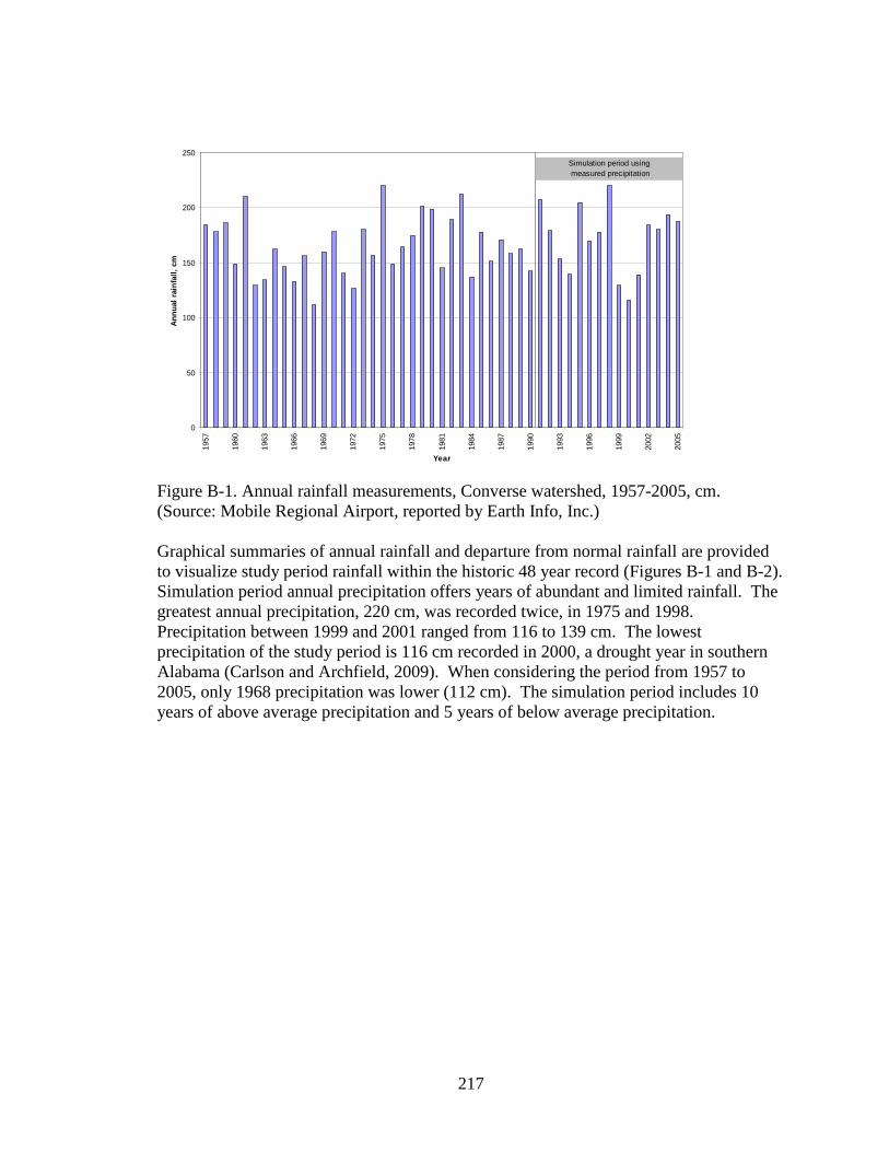
217
0
50
100
150
200
250
1957
1960
1963
1966
1969
1972
1975
1978
1981
1984
1987
1990
1993
1996
1999
2002
2005
Year
Annu
al ra
infa
ll, c
mSimulation period using measured precipitation
Figure B-1. Annual rainfall measurements, Converse watershed, 1957-2005, cm. (Source: Mobile Regional Airport, reported by Earth Info, Inc.) Graphical summaries of annual rainfall and departure from normal rainfall are provided to visualize study period rainfall within the historic 48 year record (Figures B-1 and B-2). Simulation period annual precipitation offers years of abundant and limited rainfall. The greatest annual precipitation, 220 cm, was recorded twice, in 1975 and 1998. Precipitation between 1999 and 2001 ranged from 116 to 139 cm. The lowest precipitation of the study period is 116 cm recorded in 2000, a drought year in southern Alabama (Carlson and Archfield, 2009). When considering the period from 1957 to 2005, only 1968 precipitation was lower (112 cm). The simulation period includes 10 years of above average precipitation and 5 years of below average precipitation.

218
1957
1958 19
5919
6019
6119
62 1963
1964
1965
1966
1967
1968
1969
1970
1971
1972
1973
1974
1975
1976
1977
1978
1979
1980
1981
1982
1983
1984
1985
1986
1987
1988 19
8919
9019
9119
9219
9319
9419
9519
96 1997
1998
1999
2000
2001
2002
2003
2004
2005
-80
-60
-40
-20
0
20
40
60
80
Dep
artu
re fr
om A
vera
ge, c
m
Simulation period using measured precipitation
year
, dep
artu
re fr
om n
orm
al
Figure B-2. Mobile Regional Airport departure from normal precipitation by year. (Source: NCDC Mobile Regional Airport precipitation, Earth Info, Inc. 2006).
JanuaryFebruary
MarchApril
MayJune
JulyAugust
SeptemberOctober
NovemberDecember
0
20
40
60
Figure B-3. Mean of Mobile Airport and Semmes AWIS total monthly rainfall (cm) from 1991 to 2005. The monthly rainfall depicted in Figure B-3 shows July as the month with the greatest median rainfall, excluding outliers. Outliers are defined as 1.5 * IQR. The outliers in

219
August and September coincide with hurricanes or tropical storms: August (2005; Hurricane Katrina), September (1998; Hurricane Georges and 2002; Tropical Storm Isadore). Other months with precipitation higher than 1.5 * IQR include December (1995 and 2002), January (1991 and 1998) and April (2005) generally due to multiple thunderstorms in the same month. There is little difference in the monthly precipitation of November to April (left) vs. May to October (right) monthly precipitation as shown in Figure B-4.
0
20
40
60
Figure B-4. Total monthly precipitation for November to April (left bar) and May to October (right bar) from 1991 to 2005.

220
Infilling missing precipitation data Hourly Mobile Regional Airport precipitation data are used to infill Semmes AWIS precipitation when data are missing (Appendix D. Missing Semmes AWIS rainfall data). Storms evident at the Mobile Regional Airport and in Crooked Creek streamflow in June 2003 and June 2004 are not detected in the Semmes AWIS precipitation data, possibly due to localized storms as no equipment malfunction was noted for the Semmes station. Hence, Mobile Regional Airport precipitation is used to simulate Crooked Creek in June 2003 and June 2004. On September 25 and 26, 2002, a storm is evident at the Semmes AWIS precipitation station and streamflow peaked at Crooked, Hamilton and Big Creek gauging stations. The storm is not detected at the Mobile Regional Airport. Semmes AWIS data for this storm are used to patch Mobile Regional Airport data. Hurricane Danny occurred on July 16-20, 1997 and produced extraordinary rainfall of 20 to 25 inches in portions of Mobile and Baldwin Counties. Mobile Regional Airport precipitation is 13 inches from July 18-20, while Semmes AWIS precipitation is 5.75 inches for the same time period. Big Creek simulation using Mobile Regional Airport precipitation during Hurricane Danny is an order of magnitude higher than measured Big Creek flow. Hence, Semmes AWIS data for Hurricane Danny are used to infill Mobile Regional Airport data for 18-20 July 1997. Crooked Creek simulation using Semmes AWIS data for Hurricane Danny is three times less than measured Crooked Creek flow. Hence, Mobile Regional Airport data are used to infill Semmes AWIS data for 18-20 July 1997. Daily Semmes precipitation data is used in time-series graphs and hourly Semmes AWIS station precipitation data are used in watershed model simulation. When Semmes station daily and hourly values are unavailable, Mobile regional airport data are used. Daily missing Semmes Data - 1 Jan 1991 to 3 March 1992 - 31 July 1996 to 3 Aug 1996 - 20 Sept 1996 - 16 October to 20 October 1996 - 8 April to 8 May 1998 Hurricanes and tropical storms Hurricanes and tropical storms influence model results. A list of hurricanes and tropical storms from 1991 to 2005 is provided in Table B-2. No Hurricanes or tropical storms are recorded from 1991 to mid-1995. The first hurricane recorded during the simulation period is Hurricane Erin in August 1995.

221
Table B-2. Hurricanes and Tropical Storms in Mobile County, AL, 1 January 1991 to 31 December 2005 (NOAA, 2010). Julian Day Date Name
1860 08/03/1995 Hurricane Erin
1921 10/03/1995 Hurricane Opal
2575 07/18/1997 Hurricane Danny
2985 09/01/1998 Hurricane
3009 09/25/1998 Hurricane Georges
3736 09/21/2000 Tropical Storm
4053 08/04/2001 Tropical Storm
4457 09/12/2002 Tropical Storm
4469 09/24/2002 Tropical Storm Isadore
4477 10/02/2002 Hurricane Lili
4748 6/30/2003 Tropical Storm Bill
5189 09/13/2004 Hurricane Ivan
5215 10/09/2004 Tropical Storm
5459 06/10/2005 Tropical Storm
5484 07/05/2005 Tropical Storm
5488 07/09/2005 Hurricane Dennis
5537 08/27/2005 Hurricane Katrina

222
Appendix C. Methods for determining future subwatershed urbanization and percent impervious area A. Future subwatershed urbanization The 1992 NLCD pre-urbanization scenario was compared with a respective future scenarios based upon the housing density forecasts of the Forests on the Edge (FOTE) project (Stein, 2006). The FOTE project was designed to identify areas of the US where private forests are likely to experience increases in housing density between 2000 and 2030. Housing density was estimated using historic and current density patterns and a forecast simulation model (Spatially Explicit Regional Growth Model – SERGoM) for each decade from 1970 to 2030 (Stein et al., 2006; Theobald, 2004). Forest to urban land conversion (1990 to 2020) was determined from GIS-based projections of the Forests on the Edge Project (FOTE), sponsored by the US Forest Service. The project focused on lands projected to shift from rural to urban use based on housing density (Stein et al. 2006). Details of the methodology from Stein et al. (2006) follow: “A 100-m spatial resolution dataset of the conterminous United States differentiating combinations of land cover and land ownership was constructed from the 1992 National Land Cover Dataset (NLCD) (Vogelmann and others 2001) and the Protected Areas Database (PAD) (DellaSala and others 2001). NLCD is a 30-m resolution, 21-class, land cover classification derived from nominal 1991 Landsat Thematic Mapper imagery and ancillary data by the U.S. Geological Survey. Housing density was estimated by drawing from historical and current housing densities at a fine resolution to examine spatial patterns of development. Using the historical and current housing density patterns as data inputs, a forecast simulation model of future housing density patterns was developed based on county-level population projections. Nationwide estimates of population and housing density were computed from the U.S. Census Bureau’s block-group and block data for 2000 (U.S. Census Bureau 2001a). To estimate current housing density patterns, housing density was computed using dasymetric mapping techniques (Theobald 2001a, in review). The Spatially Explicit Regional Growth Model (SERGoM v1) was used to model the full urban-to-rural spectrum of housing densities. It uses a supply-demand-allocation approach and assumes that future growth patterns will be similar to those found in the past decade. Four basic steps are used in SERGoM v1 to forecast future patterns on a decadal basis. First, the number of new housing units in the next decade is forced to meet the demands of the projected county-level population. Population growth was converted to new housing units by the county-specific housing unit per population ratio for 2000. Population estimates were obtained from a demographic-econometric model (NPA Data Services 2003). Second, a location-specific average growth rate from the previous to current time step (for example, 1990 to 2000) was computed for each of four density

223
classes: urban, suburban, exurban, and rural. These growth rates were computed for each 100 m cell using a moving neighborhood (radius = 1.6 km) that allows within-county heterogeneity and cross-county and State boundary growth patterns to be captured. Also, new housing units were spatially allocated based on these locally determined growth rates, which assumes that areas of future growth are likely to be near current high-growth areas or “hot spots.” Third, the distribution of new housing units was adjusted according to accessibility to the nearest urban core area. That is, urbanization and conversion to urban and exurban land use typically occurs at locations on the fringe of urban core areas where land is undeveloped. Accessibility is computed in terms of minutes of travel time from urban core areas as one would travel along the main transportation network.” Private forest lands were denoted “urban” if they contained 24.7 or more housing units per square km (1 or more housing units per 10 acres) (Stein et al. 2006). The spatially explicit regional growth model (SERGoM) was used to forecast 11 classes of future housing density listed below (Table C-1). Table C-1: FOTE project housing density classes Class Description from metadata Use 0 Undeveloped/private forests Rural 1 > 80 acres/unit Rural 2 50-80 acres/unit Rural 3 40-50 acres/unit Rural 4 30-40 acres/unit Rural 5 20-30 acres/unit Rural 6 10-20 acres/unit Rural 7 1.7 – 10 acres/unit Suburban 8 0.6 – 1.7 acres/unit Urban 9 < 0.6 acres/unit Urban 10 no houses, but commercial/ built up Urban Based upon the data classification, classes 7 to 10 in the FOTE were considered urban or suburban. The data were downloaded from http://www.nrel.colostate.edu/ftp/theobald/. The data are available by decade from 1970 to 2030; 2020 was selected as the future scenario to coincide with the county level projections of Wear and Greis. Future scenario methods and results (1990 to 2020): 1. Created subwatersheds shapefile for LSPC modeling which separates lands owned by MAWSS from changeable land. 2. Tabulate areas by watershed for 1990 and 2020 FOTE scenarios.

224
The ‘tabulate area’ command produces the housing density values for each subbasin. In the example above, bhc1990 is the 1990 housing density.
3. Determined urban areas for each watershed. Class 7 is considered suburban area. Classes 8 to 10 are added together and considered urban area for watershed modeling purposes. The housing density for Classes 7 to 10 is described below:
Class 7 = 1.7 – 10 acres/unit (simulate as urban, pervious in LSPC) Class 8 = 0.6 – 1.7 acres/unit (simulate as urban, impervious in LSPC) Class 9 = < 0.6 acres/unit (simulate as urban, impervious in LSPC) Class 10 = no houses, but commercial/ built up (urban, impervious)
4. Subtract 1990 urban housing density from 2020 urban housing density (in square
meters) to determine watersheds with the greatest increase in urban or suburban area.
5. Calculate percent change for each watershed (area/total change) 6. Exclude subwatersheds owned by MAWSS. 7. Evaluate 1992 forest land in each of the urbanizing watersheds (Table E-2) to ensure
the forest to urban conversion predicted is not greater than available forest land.
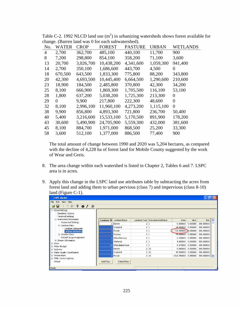
225
Table C-2. 1992 NLCD land use (m2) in urbanizing watersheds shows forest available for change. (Barren land was 0 for each subwatershed). No. WATER CROP FOREST PASTURE URBAN WETLANDS 4 2,700 362,700 485,100 440,100 11,700 900 8 7,200 298,800 854,100 358,200 71,100 3,600 13 20,700 3,026,700 10,438,200 4,341,600 1,059,300 941,400 14 2,700 350,100 1,686,600 443,700 4,500 0 18 670,500 643,500 1,833,300 775,800 88,200 343,800 20 42,300 4,693,500 10,445,400 6,664,500 1,290,600 210,600 23 18,900 184,500 2,485,800 370,800 42,300 34,200 25 8,100 666,900 1,869,300 1,705,500 116,100 53,100 28 1,800 637,200 5,038,200 1,725,300 213,300 0 29 0 9,900 217,800 222,300 48,600 0 32 8,100 2,996,100 11,960,100 4,273,200 1,115,100 0 38 9,900 856,800 4,893,300 721,800 236,700 50,400 40 5,400 3,216,600 15,533,100 5,170,500 891,900 178,200 43 30,600 5,490,900 24,705,900 5,559,300 432,000 381,600 45 8,100 884,700 1,971,000 868,500 25,200 33,300 58 3,600 512,100 1,377,000 886,500 77,400 900
The total amount of change between 1990 and 2020 was 5,204 hectares, as compared with the decline of 4,228 ha of forest land for Mobile County suggested by the work of Wear and Greis.
8. The area change within each watershed is listed in Chapter 2, Tables 6 and 7. LSPC area is in acres.
9. Apply this change in the LSPC land use attributes table by subtracting the acres from
forest land and adding them to urban pervious (class 7) and impervious (class 8-10) land (Figure C-1).

226
Figure C-1. Image of LSPC GUI land use attributes showing where land use change is applied in the watershed model.
Additional information sources: Southern Forests Resource Assessment provides county level land use change forecasts from 1992 to 2020 and 2040 (Wear & Greis 2002). The future projections are provided as county level percentages based upon the methods of Hardie and others (Hardie et al. 2000). Mobile County (FIPS Code 1097) percent changes in land use from 1992 to 2020: urban area will increase by 23% of 1992 values, agricultural area will decrease 4% of 1992 values and forest area will decrease 16% of 1992 values. According to future forecasts, urbanization is concentrated in three large areas in the Southeastern United States, one of which is the portion of the Gulf Coast centered on Mobile Bay. Applying the county level forest decline percentage (-16.5%) to the Converse watershed indicates that 4,228 ha of forest land will become urban land in the watershed. This number is used to evaluate the forest to urban land use change in Converse watershed based upon the ‘Forests on the Edge’ projections. B. Pervious/impervious designation for each urban land use classification
Urban land is partitioned into pervious or impervious land in LSPC. For the 1992 pre-urbanization scenario, pervious and impervious land is partitioned for each developed Anderson level 2 class (21, 22 and 23). Allocating pervious and impervious land for 1992 NLCD classes in the mid-Atlantic region, researchers developed three categories of development with the least developed being < 18%. All subwatersheds draining to Converse Reservoir are within the least developed category. Coefficients for percent imperviousness for the least developed category are 18.4% (class 21), 69.1% (class 22) and 34.4% (class 23) (Jennings et al., 2004). General impervious cover assumptions from another study are greater 40% (class 21), 60% (class 22) and 90% (class 23) (Bird et al., 2002). Simulation of the Neuse River watershed with LSPC, modelers partitioned urban impervious land as 12% (class 21), 65% (class 22) and 85% (class 23) (Shen et al., 2005). Impervious land cover for 1992 are provided in Tables C-4 and C-5. For the future scenarios, a decision had to be made about how much suburban and urban land would be allocated to pervious and impervious classes within the model. FOTE suburban land (class 7) is defined as 1.7 to 10 acres unit-1. This generally corresponds with the NLCD 2001 class 21 (Developed, open space), which has impervious surface area less that 20% of total cover (USGS, 2008a). For watershed modeling, acres changed to suburban land use (class 7) are partitioned as 90% pervious and 10% impervious. FOTE urban land [classes 8 to 10 (< 0.243 – 0.689 ha unit-1)] corresponds with NLCD classes 22, 23 and 24. The range of impervious cover for these classes is 20 to 100%. Given this broad range, acres changed to urban land use in the future scenarios (class 8 – 10) are allocated as 40% urban pervious land and 60% urban impervious land.

227
C-3. 1992 MRLC classifications, class names and percentage impervious utilized for each class in the LSPC model. 1992 classification
Classification name
Percentage impervious
Class 21 Low intensity residential
12% a
Class 22 High intensity residential
65% a
Class 23 Commercial/ Industrial/ transportation
85% a
Class 33 Transitional
10% a
a same as (Shen et al., 2005) Table C-4. 1992 percent impervious area applied to LSPC. Data are stored in an Access database and used by the model.

228
Appendix D. Land use change by subwatershed for base and future scenarios. Table D-1 shows land use and land use change by subwatershed. Acres changed per subwatershed are highlighted. Only subwatersheds with land use change are shown.
Land Use Subwatershed number
BASE 1992
FUTURE 1992
Barren 4 0 0 Cropland 4 89.63 89.63 Forest 4 119.87 0 Pasture 4 108.75 108.75 Urban Pervious 4 2.6 110.6 Wetlands 4 0.22 0.22 Urban Impervious 4 0.29 12.26 Barren 8 0 0 Cropland 8 73.83 73.83 Forest 8 211.05 208.55 Pasture 8 88.51 88.51 Urban Pervious 8 15.81 16.81 Wetlands 8 0.89 0.89 Urban Impervious 8 1.76 3.26 Barren 13 0 0 Cropland 13 747.91 747.91 Forest 13 2579.3 755.62 Pasture 13 1072.8 1072.83 Urban Pervious 13 217.88 1701.88 Wetlands 13 232.62 232.62 Urban Impervious 13 43.88 383.56 Barren 14 0 0 Cropland 14 86.51 86.51 Forest 14 416.77 414.27 Pasture 14 109.64 109.64 Urban Pervious 14 0.83 1.83 Wetlands 14 0 0 Urban Impervious 14 0.28 1.78 Barren 18 0 0 Cropland 18 159.01 159.01 Forest 18 453.02 114.52 Pasture 18 191.7 191.7 Urban Pervious 18 18.94 320.94 Wetlands 18 84.95 84.95 Urban Impervious 18 2.86 39.36 Barren 20 0 0 Cropland 20 1159.8 1159.78 Forest 20 2581.1 965

229
Land Use Subwatershed number
BASE 1992
FUTURE 1992
Pasture 20 1646.8 1646.83 Urban Pervious 20 238.42 1578.42 Wetlands 20 52.04 52.04 Urban Impervious 20 80.49 356.59 Barren 23 0 0 Cropland 23 45.59 45.59 Forest 23 614.25 233.75 Pasture 23 91.63 91.63 Urban Pervious 23 9.03 352.03 Wetlands 23 8.45 8.45 Urban Impervious 23 1.42 38.92 Barren 25 0 0 Cropland 25 164.79 164.79 Forest 25 461.91 135.71 Pasture 25 421.44 421.44 Urban Pervious 25 22.9 315.9 Wetlands 25 13.12 13.12 Urban Impervious 25 5.79 38.99 Barren 28 0 0 Cropland 28 157.46 157.46 Forest 28 1245 513.56 Pasture 28 426.33 426.33 Urban Pervious 28 44.23 700.23 Wetlands 28 0 0 Urban Impervious 28 8.47 83.91 Barren 29 0 0 Cropland 29 2.45 2.45 Forest 29 53.82 51.32 Pasture 29 54.93 54.93 Urban Pervious 29 8.61 9.61 Wetlands 29 0 0 Urban Impervious 29 3.4 4.9 Barren 32 0 0 Cropland 32 740.35 740.35 Forest 32 2955.4 1116.89 Pasture 32 1055.9 1055.93 Urban Pervious 32 227.74 1820.74 Wetlands 32 0 0 Urban Impervious 32 47.81 293.32 Barren 38 0 0 Cropland 38 211.72 211.72 Forest 38 1209.2 724.86 Pasture 38 178.36 178.36

230
Land Use Subwatershed number
BASE 1992
FUTURE 1992
Urban Pervious 38 52.47 488.47 Wetlands 38 12.45 12.45 Urban Impervious 38 6.02 54.36 Barren 40 0 0 Cropland 40 794.84 794.84 Forest 40 3838.3 0 Pasture 40 1277.7 1277.65 Urban Pervious 40 196.01 3650.01 Wetlands 40 44.03 44.03 Urban Impervious 40 24.39 408.69 Cropland 43 1356.8 1356.83 Forest 43 6104.9 5482.24 Pasture 43 1373.7 1373.73 Urban Pervious 43 93.23 647.23 Wetlands 43 94.3 94.3 Urban Impervious 43 13.52 82.18 Barren 45 0 0 Cropland 45 218.61 218.61 Forest 45 487.04 7.64 Pasture 45 214.61 214.61 Urban Pervious 45 5.44 436.44 Wetlands 45 8.23 8.23 Urban Impervious 45 0.79 49.19 Barren 58 0 0 Cropland 58 126.54 126.54 Forest 58 340.26 85.76 Pasture 58 219.06 219.06 Urban Pervious 58 16.97 244.97 Wetlands 58 0.22 0.22 Urban Impervious 58 2.15 28.65

231
Appendix E. Nutrient concentrations below the detection limit used for watershed calibration and validation. When nutrient concentrations are below the detection limit, the detection limit is used to estimate the concentrations. Total phosphorus (parameter code 665) analytical methods changed three times during the study period, resulting in different detection limits for TP. The detection limit is <0.01 during 1990-91; <0.02 during 92-98; <0.002 from 99-04. Big Creek TP concentrations were below detection 28 of 70 samples between 1990 and 2004. Crooked Creek TP concentrations were below the detection level in 24 of 70 samples. Hamilton Creek TP concentrations were below detection in 30 of 70 samples. Total nitrogen is the sum of unfiltered ammonia in mg L-1 (610), organic nitrogen in mg L-1 (625-610) and nitrate plus nitrite in mg L-1 (630). The number of samples below detection limit is listed in Table x. Table E-1. Number of samples below detection limit for TN components at Big, Crooked and Hamilton Creeks, 1990 to 2005
USGS parameter number
Big Creek Crooked Creek Hamilton Creek
Detection limit
610 3 10 5 < 0.01 625 14 23 31 <0.20 630 2 1 0 <0.02
The detection limit for total organic carbon is 0.1 mg L-1. No Big Creek or Hamilton Creek samples were below detection for TOC. Crooked Creek had one TOC sample below the detection limit on 23 July 1997.

232
Appendix F. Equations used in statistical analyses Moriasi et al. (2007) provide guidance for evaluation of watershed model performance. The authors recommend the use of graphical techniques, along with NSE, RSR and PBIAS and provide performance ratings using monthly data. Donigian (2002) provides performance ratings for the ratio of simulated and recorded values. Nash-Sutcliffe efficiency (NSE): “The Nash-Sutcliffe efficiency (NSE) determines the relative magnitude of the residual variance (“noise”) compared to the measured data variance (“information”) (Nash and Sutcliffe, 1970). NSE indicates how well the plot of observed versus simulated data fits the 1:1 line.”
NSE ranges between - infinity and 1.0 (1 inclusive), with NSE = 1 being the optimal value. Values between 0.0 and 1.0 are generally viewed as acceptable levels of performance, whereas values <0.0 indicates unacceptable performance. Percent bias (PBIAS): Percent bias (PBIAS) measures the average tendency of the simulated data to be larger or smaller than observed data. The optimal value of PBIAS is 0.0. Positive values indicate model underestimation bias, and negative values indicate model overestimation bias.
Ratio of the root mean square error to the standard deviation of measured data (RSR): RSR standardizes the root mean squared error statistic using the observations standard deviation. The optimal value for RSR is zero.
Absolute Mean Error (AME): AME gives an indication of how close the observed values are to the predicted values.

233
Fractional absolute mean error is the ratio of the AME to the mean of observations expressed as a percent. The FMAE is the best statistic to use to make comparisons of model performance between other study results since it has been normalized (Tillman et al, 2004).
Donigian (2002) provides ranges for calibration model performance based upon the ratio of simulated and observed means.
Percent difference is used to compare future and pre-urbanization scenario total and median results using the formula below.

234
Appendix G. LSPC hydrologic and water quality parameters and final values Hydrologic parameters
Monthly values are utilized for interception storage capacity (CEPSC; in), upper zone nominal storage (UZSN; in) and the lower zone evapotranspiration parameter (LZETP; unitless) in the Converse model. CEPSC is the amount of rainfall retained by vegetation which is eventually evaporated. The maximum interception value suggested by Donigian and Davis (1978) is 0.20 in for forest. Values are within guidelines (EPA, 2000) and Converse model CEPSC values ranged from 0.01 in on barren land in the winter to 0.15 in on forest land in the summer, all well within recommended guidelines (EPA, 2000). Although interception storage capacity varies by land use and month, the same CEPSC values are used in each watershed. For example, barren land is given the same CEPSC in Big, Hamilton and Crooked Creek watersheds.
Upper zone soil moisture storage (UZSN; in) values are a function of surface soil conditions and account for near surface water retention. A large UZSN value increases the amount of water retained in the upper zone and available for evapotranspiration and reduces overland flow. Calibrated UZSN values range from 0.1 in on barren land to 2.0 in on forest land and are within published guidelines (EPA, 2000).
LZETP (unitless) is the index to lower zone evapotranspiration or a coefficient to define the ET opportunity. It is primarily a function of vegetation and the maximum values range from 0.1 to 0.9. Monthly calibrated LZETP values are 0.001 for barren and urban impervious land. Pervious urban land LZETP is 0.1 for each month. Values for forest, crop, pasture and wetland LZETP vary monthly and range from 0.1 to 0.7.
LZSN (in) is the lower zone nominal soil moisture storage is related to precipitation and soil characteristics of the region. The possible range is 2.0 to 15.0 in. The Agricultural Runoff Model (ARM) user’s manual includes a map of calibrated LZSN values across the country and indicates a value of 6.0 for the Converse Watershed (Donigian and Davis, 1978). Viessman et al. (1989) provide an initial estimate of LZSN for coastal, humid climates as one-eighth annual rainfall plus 4 in, which is approximately 12 in for Converse watershed. Final calibrated LZSN is 9 in for each land use in Big and Crooked Creek watersheds. Hamilton Creek final calibrated LZSN is 7 in for each land use.
Infiltration (INFILT; in hr-1) is the index to mean soil infiltration rate. INFILT divides the surface and subsurface flow. High values produce more water in the lower zone and higher baseflow. INFILT is not an infiltration capacity and values are normally much less than published infiltration rates from the literature (EPA, 2000). Model values for INFILT are greatest on forest land, ranging from 0.35 to 0.41 in hr-1, less than the maximum recommended value of 0.50 in hr-1 (EPA, 2000). Crop and pasture land INFILT are between 0.15 and 0.33 in hr-1. The smallest INFILT is 0.01 in hr-1 on urban impervious land. While INFILT cannot be compared with infiltration capacity values, high model INFILT values are supported by field observations. Converse watershed soils are highly permeable and water infiltrates rapidly (Gillett et al., 2000). Streams draining the Citronelle formation, such as those within the Converse watershed, had the highest low water yields per square mile of drainage area in Alabama (Pierce, 1966). An infiltration exponent of 1.5 (unitless), rather than the typical 2.0, is used for Big and Crooked Creek watersheds to allow for greater mean and maximum infiltration

235
capacities. The infiltration equation is provided in the HSPF user manual (Bicknell et al., 2001).
BASETP (unitless) is the evapotranspiration by riparian vegetation and if significant riparian vegetation exists in the watershed, then nonzero values should be used. Adjustments are visible in the low flow simulation. Possible BASETP values range from 0.00 to 0.20. A BASETP value of 0.03 is used for forestland in Hamilton and Crooked Creek watersheds. Big Creek BASETP is 0.05 for crop and pasture land use and 0.15 for forestland.
AGWETP (unitless) refers to evapotranspiration from groundwater storage, such as wetlands or marsh areas. Since wetlands are represented in the model, AGWETP is zero for all land use classifications other than wetlands and a relatively high value for wetlands. Calibrated AGWETP values range from 0.1 to 0.3.
DEEPFR (unitless) is the fraction of infiltrating water lost to deep aquifers, with the remaining water as active groundwater storage that contributes to baseflow. Watershed areas in the upland portion of the watershed are more likely to loose more water to deep groundwater. This is the case in Converse Watershed, wherein Big and Crooked Creek DEEPFR is 0.18 for crop and pasture land and 0.24-0.34 for forest land. None of the Hamilton Creek infiltrating water is lost through deep percolation.
Initial interflow inflow parameter (INTFW) estimates from a national map of interflow values are 2.0 (unitless) for Converse watershed (Donigian and Davis, 1978). Calibrated Crooked and Hamilton Creek interflow values ranged from 0.5 to 2.0. Big Creek interflow values ranged from 0.5 to 5.0 (unitless).
Groundwater recession rate (AGWRC; d -1) values for Converse watershed range from 0.991 to 0.998 d -1. This parameter controls the baseflow recession. AGWRC influences the active groundwater outflow, and a larger value for AGWRC decreases the active groundwater outflow. AGWRC generally ranges from 0.92 to 0.99 d -1. The high calibrated AGWRC values at Converse watershed are similar to the values of other studies. AGWRC is 0.996 d -1 for high density forest in Oregon (USEPA, 2000).
Interflow recession coefficient (IRC; unitless) affects the rate at which interflow is discharged from storage. IRC generally ranges from 0.3 to 0.85 with values near the high end resulting in slower interflow discharge. Calibrated IRC in Hamilton Creek watershed is 0.3 resulting in rapid interflow discharge. An intermediate value of 0.6 characterizes forest and agricultural land in Crooked and Big Creek watersheds. The remaining land uses in Crooked and Big Creek watersheds have an IRC of 0.3 to 0.4. Water quality parameters Total Phosphorus parameters
Calibrated TP ACQOP values ranged from 0.004 lb ac-1 d-1 on barren land to 0.02 lb ac-1 d-1 on urban impervious land. These accumulation rates are slightly greater than rates reported for a calibrated Mobile Bay LSPC model (0.0005 lb ac-1 d-1 to 0.01 lb ac-1 d-1 (Childers, 2009) and near the estimated TP accumulation values for the St. Lawrence River basin (0.001 to 0.018 lb ac-1 d-1) (Macdonald and Bennett, 2009).
Values from previous models listed below provide an initial estimate that ACQOP is between 0.0005 and 0.018 lb acre-1 d-1. Phosphate (PO4) ACQOP for a model of the Patuxent watershed ranged from 0.001 to 0.005 lb acre-1 d-1 (USEPA, 2009). TP

236
accumulation rate ranged from 0.0005 lb acre-1 d-1 for agricultural land to 0.01 lb acre-1 d-
1 for urban impervious land in a calibrated LSPC model for Mobile Bay (Childers, 2009). TP accumulation for agricultural land in the St. Lawrence River basin ranged from 0.001 to 0.018 lb acre-1 d-1 (Macdonald and Bennett, 2009).
The calibrated TP maximum surface storage (SQOLIM) ranged from 0.008 to 0.034 lb ac-1. Measured values fall within this range as the mean soil phosphorus content under pine and spruce trees is 0.018 lb ac-1 at 0.1 mm depth (Alban et al., 1982). TP SQOLIM values for an LSPC simulation of the Maryland piedmont near Washington, D.C. (0.080 to 0.132 lb acre-1) were greater than Converse SQOLIM (Brubaker et al, 2008). TP SQOLIM values for an LSPC simulation of Mobile Bay (0.001 to 0.02 lb ac-1) were less than Converse SQOLIM (Childers, 2009). Converse TP WSQOP is 0.9 in hr-1. The total phosphorus content for the soil (30 cm depth) in the nutrient poor Igapó watershed of the Brazilian Amazon is 430 kg ha-1 which is converted to 0.13 lb acre-1 at 0.1 mm depth to estimate SQOLIM (Furch, 1997).
In previous models, the rate of surface runoff that removes 90% of the stored parameter (WSQOP) ranges from 0.50 in hr-1 in the Patuxent watershed to 1.64 in hr-1 for West Sandy Creed. An intermediate value of 0.70 in hr-1 is reported for Blue Earth River, MN. A calibrated value of 1.2 in hr-1 for the Mobile Basin is reported and used as a starting point in the Converse model (Childers, 2009).
Calibrated TP interflow concentration ranges from 0.001 mg L-1 on barren land to 0.1 mg L-1 on crop land. Calibrated TP groundwater concentration ranges from 0.001 mg L-1 on barren land to 0.03 mg L-1 on crop and urban land. Interflow and groundwater concentrations are within the measured groundwater TP in the Mobile River basin, which ranged from <0.006 to 0.3 mg L-1 (Robinson, 2003). TP in groundwater is generally less than 0.1 mg L-1 (Robinson, 2003; Raghunathan et al., 2001). In the Patuxent watershed, interflow phosphate concentrations ranged from 0.005 mg L-1 for forest and wetland land use to 0.055 mg L-1 for commercial and industrial land use. Groundwater phosphate concentrations in the same simulation are an order of magnitude less, ranging from 0.001 mg L-1 for forest land to 0.005 for commercial and industrial land (USEPA, 2009). Interflow TP in the calibrated Mobile Bay model ranged from 0.001 mg L-1 for barren land to 0.1 mg L-1 for crop land. Groundwater TP concentrations are between 0.001 and 0.05 mg L-1 (Childers, 2009). Total soluble phosphorus, which is filtered before analysis, at the West Walker Branch watershed for riparian groundwater and spring water is near 0.007 mg L-1 (Mulholland, 1992). This watershed is similar to the Converse watershed in that infiltration is high and available nutrients are low. Based upon this finding for soluble phosphorus, which is filtered prior to analysis, TP concentrations for Converse interflow and groundwater can be assumed to be greater than 0.007 mg L-1. Total Nitrogen
Calibrated Converse watershed TN values for ACQOP, SQOLIM and WSQOP mimic values used in the Mobile Bay LSPC model (Childers, 2009). Corresponding TN ACQOP ranged from 0.01 lb ac-1 d-1 on forest land to 0.6 lb ac-1 d-1 in urban pervious land and TN SQOLIM ranged from 0.01 to 1.20 lb ac-1. Measured TN content to 30 cm depth in the Igapo and Varzea is 7610 to 5907 kg ha-1, respectively (Furch, 1997). These are converted to a depth of 0.1 mm to estimate surface storage values of 2.3 to 1.8 lb acre-

237
1. These measured surface storage values are greater than the LSPC calibrated storage values for Converse watershed.
TN WSQOP ranges from 0.8 in hr-1 on barren, pasture and urban land to 1.3 in hr-
1 on forest and wetland parcels. Interflow and groundwater TN concentrations range from 0.05 mg L-1 on barren land to 2 mg L-1 on urban land. Mobile basin median measured urban groundwater TN concentrations of 2.0 mg L-1 are used in the Converse model (Robinson, 2003). Mulholland (1992) measured forested watershed nitrogen concentrations in riparian groundwater (interflow) and spring water (groundwater) and found total nitrogen values of approximately 0.105 mg L-1 and 0.085 mg L-1, respectively. Calibrated input forest interflow and groundwater TN values (0.5 mg L-1) are greater than Mulholland’s measured values, but less than the values used to simulated the Patuxent River watershed (NO3 + NH4 = 0.67 to 0.87 mg L-1) (USEPA, 2009).
Total Organic Carbon Carbon ACQOP values ranged from 1.05 lb ac-1 d-1 on barren and urban land use to 4.9 lb ac-1 d-1 in wetlands. A national model of carbon flux from 2001 to 2005 provides general guidance for the carbon accumulation rate in Converse watershed (Peters et al., 2007). A general estimate of carbon accumulation of 0.7 lb ac-1 d-1 is reported. Reported carbon accumulation rates are higher (4.9 lb ac-1 d-1) for everglades wetlands (Reddy et al, 1993). Calibrated TOC SQOLIM ranges from a minimum of 2.14 lb ac-1 on crop land to a maximum of 31.23 lb ac-1 in wetlands. These values are determined using carbon storage estimates by land use (converted to 0.1 mm depth) for the south central region (Pouyat et al., 2006). Calibrated TOC WSQOP is 1.7 in hr-1. Calibrated TOC interflow concentrations range from 1.2 mg L-1 on barren land to 6.2 mg L-1 in wetlands. Groundwater TOC concentrations are lower, ranging from 1.1 mg L-1 to 4.8 mg L-1. Mobile basin median measured urban groundwater DOC concentrations are 0.28 mg L-1 (Robinson, 2003). Since the model is simulating TOC, which is greater than DOC, values of 1.28 mg L-1 are used for urban land use.

238
Appendix H. Evaluation of watershed model concentration data distribution Histograms and quantile-quantile (Q-Q) plots of TN, TP and TOC concentrations at Big Creek, the largest tributary to Converse Reservoir, are utilized to analyze data distribution. Residuals (observed value – mean of observed values) of daily results (1991 – 2005; n=5,478) for TN, TP and TOC from LSPC simulation using 1992 MRLC were used to evaluate whether or not data conform to a normal distribution (Figures H-1 to H-3). The histograms indicate that TN, TP and TOC concentrations are not normally distributed. Q-Q normal plots also indicate LSPC concentrations do not follow a normal distribution (Figures H-4 to H-6). Based upon these graphs, TN, TP and TOC concentration data are analyzed using nonparametric statistics.

239
-0.07 0.07 0.20 0.34 0.47 0.61 0.74 0.88 1.01 1.15 1.28TN residuals
0
1000
2000
3000
4000
Figure H-1. Histogram of TN residuals
-4 -2 0 2 4Normal Distribution
-0.1
0.3
0.7
1.1
TN re
sidu
als
Figure H-4. Q-Q normal plot of TN residuals
-0.007 -0.002 0.003 0.008 0.013 0.018 0.023 0.029 0.034 0.039 0.044TP residuals
0
500
1000
1500
2000
2500
Figure H-2. Histogram of TP residuals
-4 -2 0 2 4Normal Distribution
-0.01
0.00
0.01
0.02
0.03
0.04
TP re
sidu
als
Figure H-5. Q-Q normal plot of TP residuals
-0.6 0.3 1.2 2.1 3.0 3.9 4.9 5.8 6.7 7.6 8.5TOC residuals
0
1000
2000
3000
Figure H-3. Histogram of TOC residuals
-4 -2 0 2 4Normal Distribution
-1
1
3
5
7
9
TOC
resi
dual
s
Figure H-6. Q-Q normal plot of TOC residuals

240
.

241
Appendix I. Evaluation of the Environmental Fluid Dynamics Code reservoir model to simulated Converse Reservoir, a public water supply impoundment in southern Alabama, USA An evaluation of the responsiveness of a reservoir model, Environmental Fluid Dynamics Code (EFDC), to changes in tributary loads to Converse Reservoir, a drinking water supply reservoir was conducted. The evaluation determines the ability of the EFDC model to simulate how changes in upstream nutrient loads influence water quality at a drinking water in-take, which is located on a tributary roughly 4.8 km from the mainstem of the reservoir. The reservoir model is then used to evaluate the influence of watershed urbanization on reservoir water quality. The goal of this analysis is to evaluate model sensitivity at the intake location to varied, but feasible, nutrient loads.
Two model simulations are performed. The first simulation utilizes actual tributary nutrient levels to determine total nitrogen, total phosphorus and total organic carbon values at the in-take which is located along a branch of the reservoir and may not be influenced by changes to the mainstem. To test this, a second simulation utilizes increased nutrient loads to the uppermost mainstem tributary. Changes in phosphorus, nitrogen and organic carbon at the in-take are compared with baseline conditions to evaluate EFDC responsiveness. Water surface elevation and nutrient results are evaluated using Nash-Sutcliffe efficiency (NSE), percent bias (PBIAS), and ratio of the root mean square error to the standard deviation of measured data (RSR).
The modeled and measured water surface elevation resulted in a very good overall performance. The predicted water surface elevation resulted in an NSE (0.98), PBIAS (0.02%) and RSR (0.12) near optimal values.
To determine model performance in simulating water quality, results from the baseline scenario at the in-take are compared with measured data at the same location. Monthly phosphorus (TP) and nitrogen (TN) samples were collected in 1991. Seventy-five percent of the TP measurements were reported as the detection limit (0.01 mg/l) while model results were all less than 0.01 mg/l, thereby limiting comparisons between measured and simulated results. PBIAS results suggest good model performance in simulating TN. NSE and RSR suggest unsatisfactory model performance for TN. TP, TN and total organic carbon concentrations at the in-take were greater during the urbanization scenario than the baseline scenario. Urban nutrient loads in the upstream most tributary increased nutrient concentrations at the drinking water intake, which is located on a tributary roughly 4.8 km from the mainstem of the reservoir. Total phosphorus and total organic carbon concentrations during the urban scenario were approximately twice baseline concentrations indicating that future watershed urbanization could adversely impact source water.

242
Appendix J. Test of the influence of initial concentrations on water quality results A test of the influence of initial concentrations on reservoir water quality at the MAWSS drinking water intake (cell 34,18) was conducted. Initial concentrations for TN, TP and TOC (Card 44) were doubled and the simulation was run for one year. Results for TN, TP and TOC are provided in Figures S-1, S-2 and S-3, respectively. Even with two times the original initial concentration, simulated TN, TP and TOC concentrations were the same as the simulation with original initial concentrations after approximately 6 months. Based upon this test, a model start-up time of at least 6 months will be allowed prior to results analysis.
TN initial concentration test
0
0.5
1
1.5
2
2.5
Jul-90 Aug-90 Sep-90 Oct-90 Nov-90 Dec-90 Jan-91 Feb-91 Mar-91 Apr-91 May-91 Jun-91
TN C
once
ntra
tion
mg
L-1
TN 2XICTN IC
Figure J-1.

243
TP initial concentration test
0
0.005
0.01
0.015
0.02
0.025
0.03
0.035
0.04
Jul-90 Aug-90 Sep-90 Oct-90 Nov-90 Dec-90 Jan-91 Feb-91 Mar-91 Apr-91 May-91 Jun-91
TP c
once
ntra
tion
mg
L-1
TP 2XICTP IC
Figure J-2.
TOC initial concentration test
0
1
2
3
4
5
6
7
8
9
Jul-90 Aug-90 Sep-90 Oct-90 Nov-90 Dec-90 Jan-91 Feb-91 Mar-91 Apr-91 May-91 Jun-91
TOC
Con
cent
ratio
n m
g L-
1
TOC 2XICTOC IC
Figure J-3.

244
Appendix K Constant EFDC outflow correction based upon simulated and measured water surface elevation. MRLC 1992 water surface elevation The future simulation for Feb 2001 to April 2005 has a linear upward trend of 0.0042 m d-1 (Figure K-1). Using the reservoir surface area of 14 500 000 m2, the constant daily outflow correction volume is 60,900 m3 (0.70 m3 s-1 or 15.9 MGD). The additional daily outflow correction of 15.9 MGD is added to the measured spillway outflow from 4 March 2001 to 30 April 2005.
y = 0.0042x + 33.128
R 2 = 0.9333
30
32
34
36
38
40
42
Feb
-01
Apr
-01
Jul-0
1
Sep
-01
Dec
-01
Mar
-02
May
-02
Aug
-02
Nov
-02
Jan-
03
Apr
-03
Jul-0
3
Sep
-03
Dec
-03
Feb
-04
May
-04
Aug
-04
Oct
-04
Jan-
05
Apr
-05
Wat
er S
urf
ace
Ele
vati
on
, m
predicted no correctionfuture92
m eas ured
predicted cons tantcorrection future92
L inear (predicted nocorrection future92)
Figure K-1. Measured water level at Converse spillway, post-urban 1992 predicted WSE using LSPC inflows and WSE with constant outflow correction for 1 February 2001 to 30 April 2005.

245
Appendix L. Values of rates and constants used in the master water quality input file. The following tables from the EFDC water quality manual provide rates and constants used in the WQ3DWC.INP water quality input file for a calibrated EFDC model of Florida Bay for comparison with Converse Reservoir values. Table L-1 Water Quality Parameters Related to Algae in the Water Column Parameter Description Florida Bay
(Cerco et al., 2000) Converse Reservoir
PMc (day-1) Maximum growth rate under optimal conditions
4.0 N/A PMd (day-1) N/A N/A PMg (day-1) N/A 3.0 KHNx (g N m-3) Half-saturation
constant for nitrogen uptake for green algal
0.03 0.01
KHPx (g P m-3) Half-saturation constant for phosphorus uptake
0.005 0.001
FD Fractional day length
1 N/A; use aser.inp
Keb (m-1) Light extinction due to water
0.13 0.4
KeISS (m-1 per g m-3) Light extinction 0.085 N/A KeVSS (m-1 per g m-3) Light extinction 0.085 N/A KeChl (m-1 / mg Chl m-
3) Light extinction due to chlorophyll
N/A Riley formula (1956)
CChlx (g C / mg Chl) Carbon-to-chlorophyll ratio
0.075 0.60
(Dopt)x (m) Optimal depth N/A 1.0 Isx (watts/meter2) Optimal light
intensity N/A N/A; use aser.inp
Isxmin (watts/meter2) Minimum light intensity
N/A 40
KHI (watts/meter2) Half saturation for light limitation
60 (E/ meter2-day) N/A
CIa, CIb & CIc Weighting factors for solar radiation
1.0, 0.0, 0.0 0.7, 0.2, 0.1
TMlowc, TMuppc (°C) 25, 25 N/A TMlowd, TMuppd (°C) N/A N/A TMlowg, TMuppg (°C) Lower and upper
optimal temperature for algae growth
N/A 28, 28

246
KTG1c , KTG2c (°C-2) 0.004, 0.012 N/A KTG1d , KTG2d (°C-2) N/A N/A KTG1g , KTG2g (°C-2) Super and sub
optimal temperature effect
N/A 0.01, 0.01
STOX (ppt) Salinity toxicity 1.0 N/A BMRc (day-1) Basal metabolism
rate 0.1 N/A
BMRd (day-1) N/A N/A BMRg (day-1) N/A 0.02 TRx (°C) Reference
temperature for metabolism
20 20
KTBx (°C-1) Temperature effect coefficient
0.0322 0.032
PRRc (day-1) Predation rate on algae
0.02 N/A PRRd (day-1) N/A N/A PRRg (day-1) N/A 0.1 WSc (m day-1) Settling velocity 0.01 N/A WSd (m day-1) N/A N/A WSg (m day-1) N/A 0.01 Table L-2 Parameters Related to Organic Carbon in the Water Column Parameter Description Florida Bay
(Cerco et al., 2000) Converse Model
FCRP Carbon distribution coefficient for algae predation – refractory particulate
0.25 0.20
FCLP 0.50 0.0 FCDP Carbon
distribution coefficient for algae predation – dissolved organic carbon
0.25 0.80
KHRx (g O2 m-3) Half saturation constant for green algae excretion
0.0 0.5
WSRP (m day-1) Settling velocity for refractory particulate organic matter
0.03 0.25
WSLP (m day-1) Settling velocity for labile
0.03 0.0

247
Parameter Description Florida Bay (Cerco et al., 2000)
Converse Model
particulate organic matter
KHORDO (g O2 m-3) Oxic respiration half-saturation constant for dissolved oxygen
0.5 0.5
KRC (day-1) Minimum dissolution rate for refractory particulate organic carbon
0.005 0.005
KLC (day-1) 0.02 N/A KDC (day-1) Minimum
dissolution rate of dissolved organic carbon
0.01 0.01
KRCalg (day-1/ g C m-3) Constant relating dissolution rate to total chlorophyll-a
0.0a 0.0 KLCalg (day-1/ g C m-3) 0.0a 0.0 KDCalg (day-1/ g C m-3) 0.0a 0.0 TRHDR (°C) Reference
temperature for hydrolysis
20.0 20.0
TRMNL (°C) Reference temperature for mineralization
20.0 20.0
KTHDR (°C-1) Temperature effect constant for hydrolysis
0.069 0.069
KTMNL (°C-1) Temperature effect constant for mineralization
0.069 0.069
AANOX Ratio of denitrification rate to oxic DOC respiration rate
0.0b 0.5
KHDNN (g N m-3) Half-saturation constant for denitrification
0.0b 0.1
a Not reported. Assumed value of zero b Not reported. Assumed no simulation of denitrification Table L-3. Parameters related to phosphorus in the water column.

248
Parameter Description Florida Bay (Cerco et al., 2000)
Converse Model
FPRP Phosphorus distribution coefficient for algae predation refractory particulate organic phosphorus
0.03 0.1
FPLP 0.07 0.0 FPDP Dissolved
organic phosphorus
0.4 0.4
FPIP Inorganic phosphorus
0.5a 0.5
FPRx 0.0 0.0 FPLx 0.0 0.0 FPDx Phosphorus
distribution coefficient of DOP for green algae metabolism
0.5 0.6
FPIx Phosphorus distribution coefficient of inorganic phosphorus for green algae metabolism
0.5a 0.4
APCx (g P per g C)
0.0167 NA
WSs(m/day) Settling velocity for particles sorbed to TAM
0.03 0.0
KPO4p(m3/g) for TSS
Partition coefficient for sorbed/dissolved PO4
0.2 1.0
CPprm1(g C per g P)
Constant used to determine algae phosphorus to carbon ratio
60 30

249
Parameter Description Florida Bay (Cerco et al., 2000)
Converse Model
CPprm2(g C per g P)
Constant used to determine algae phosphorus to carbon ratio
0 b 20
CPprm3 (per g P m-
3) Constant used to determine algae phosphorus to carbon ratio
0 b 350
KRP(day-1) Minimum hydrolysis rate for particulate organic phosphorus
0.005 0.01
KLP(day-1) 0.12 0.0 KDP(day-1) Minimum
hydrolysis rate for dissolved organic phosphorus
0.2 0.1
KRPalg(day-1 per g C m-3)
0.2 0.0
KLPalg(day-1 per g C m-3)
0.0b 0.0
KDPalg(day-1 per g C m-3)
Constant relating hydrolysis rate of algae to dissolved phosphorus
0.0b 0.5
a Not reported. Value inferred from constraint. b Not reported. Value assumed to be zero.
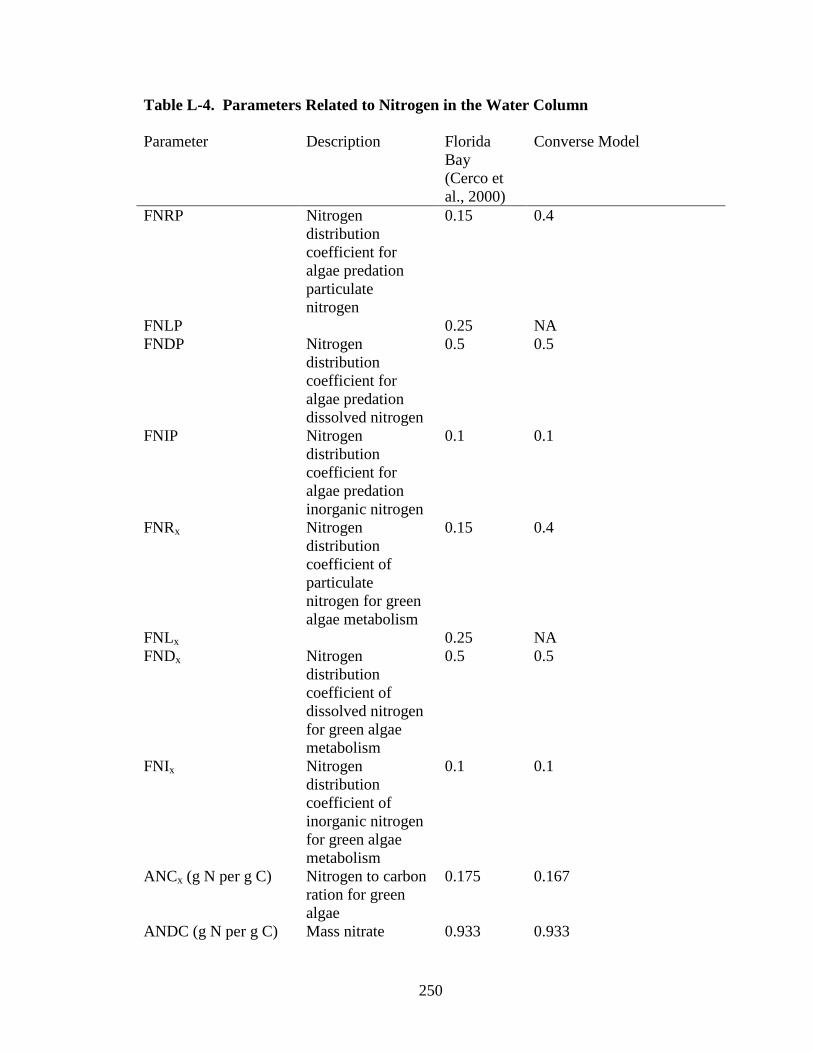
250
Table L-4. Parameters Related to Nitrogen in the Water Column Parameter Description Florida
Bay (Cerco et al., 2000)
Converse Model
FNRP Nitrogen distribution coefficient for algae predation particulate nitrogen
0.15 0.4
FNLP 0.25 NA FNDP Nitrogen
distribution coefficient for algae predation dissolved nitrogen
0.5 0.5
FNIP Nitrogen distribution coefficient for algae predation inorganic nitrogen
0.1 0.1
FNRx Nitrogen distribution coefficient of particulate nitrogen for green algae metabolism
0.15 0.4
FNLx 0.25 NA FNDx Nitrogen
distribution coefficient of dissolved nitrogen for green algae metabolism
0.5 0.5
FNIx Nitrogen distribution coefficient of inorganic nitrogen for green algae metabolism
0.1 0.1
ANCx (g N per g C) Nitrogen to carbon ration for green algae
0.175 0.167
ANDC (g N per g C) Mass nitrate 0.933 0.933

251
Parameter Description Florida Bay (Cerco et al., 2000)
Converse Model
reduced per D OC oxidized
KRN (day-1) Minimum hydrolysis rate for particulate organic nitrogen
0.005 0.009
KLN (day-1) 0.03 N/A KDN (day-1) Minimum
hydrolysis rate for dissolved organic nitrogen
0.01 0.01
KRNalg (day-1 /g C m-3) Constants relating hydrolysis rate to algae
0.0a 0
KLNalg (day-1 /g C m-3) 0.0a 0 KDNalg (day-1 /g C m-3) 0.0a 0 Nitm (g N m-3 day-1) Maximum
nitrification rate 0.01 0.35
KNit (day-1) 0.01 KHNitDO (g O2 m-3) Nitrification half-
saturation constant for dissolved oxygen
3.0 1.0
KHNitN (g N m-3) Nitrification half-saturation constant for NH4
1.0 1.0
TNit1 (°C) Reference temperature for nitrification
30 55
KNit1 (°C-2) Suboptimal temperature effect constant
0.003 0.0012
KNit2 (°C-2) Superoptimal temperature effect constant for nitrification
0.003 0.0012
a Not reported. Assumed value of zero.

252
Table L-5 Parameters Related to Chemical Oxygen Demand and Dissolved Oxygen in the Water Column Parameter Description Florida
Bay (Cerco et al., 2000)
Converse Model
KHCOD (g O2 m-3) Oxygen half-saturation constant for COD decay
0.5 1.5
KCD (day-1) COD decay rate 20 1.0 TRCOD (°C) Reference
temperature for COD decay
20a 20
KTCOD (°C-1) Temperature rate constant for COD decay
0.069a 0.041
AOCR (g O2 per g C) Stoichiometric algae oxygen to carbon ratio
2.67 2.67
AONT (g O2 per g N) Stoichiometric algae oxygen to nitrogen ratio
4.33 4.33
Kro (in MKS unit) Reaeration constant
3.933 3.933
KTr Temperature rate constant for reaeration
20 1.024

253
Appendix M Methods used to analyze Converse Reservoir data collected by AU, MAWSS, and USGS. Table M-1 provides the analytical methods used in chemical analysis by USGS and Dr. Bayne, Fisheries and Allied Aquaculture at Auburn University. Collected data were used in watershed and reservoir model calibration and validation. USGS methods are available on-line (USGS, 2009). The methods used by Dr. Bayne’s laboratory are provided in the Limnological Study of Big Creek (Bayne et al., 1998). MAWSS provided TOC data collected at the source water intake and analytical methods directly. Most of the TOC is analyzed using the same method. Only the AU laboratory TOC data (n=12) collected in 1997 uses a different method. Nitrate, nitrite, total and dissolved phosphorus are analyzed using the same methods regardless of sampling entity. Table M-1. Analytical methods AU METHODS
(APHA, 1995) USGS METHODS
Ammonia (USGS code 610 and 608)
Phenate method Colormetric, salicylate-hypochlorite, automated segmented flow
Ammonia plus organic nitrogen (USGS code 623 and 625)
Micro Kjeldahl colorimetric, block digestor-salicylate-hypochlorite, automated-segmented flow
Nitrite (USGS code 613 and 615)
Diazotization Colorimetric, diazotization, automated-segmented flow
Nitrite plus nitrate (USGS code 631 and 630)
Cadmium reduction (nitrate only)
Colorimetric, cadmium reduction-diazotization, automated-segmented flow
Dissolved and total phosphorus as P (USGS code 666 and 665)
Persulfate digestion, ascorbic acid
Colorimetric, phosphomolybdate, automated-segmented flow
Dissolved and total orthophosphate (USGS code 671 and 70507)
NA colorimetric, phosphomolybdate, automated-segmented flow
Soluble reactive phosphorus
Ascorbic acid NA
Total organic Persulfate- ultraviolet 5310B
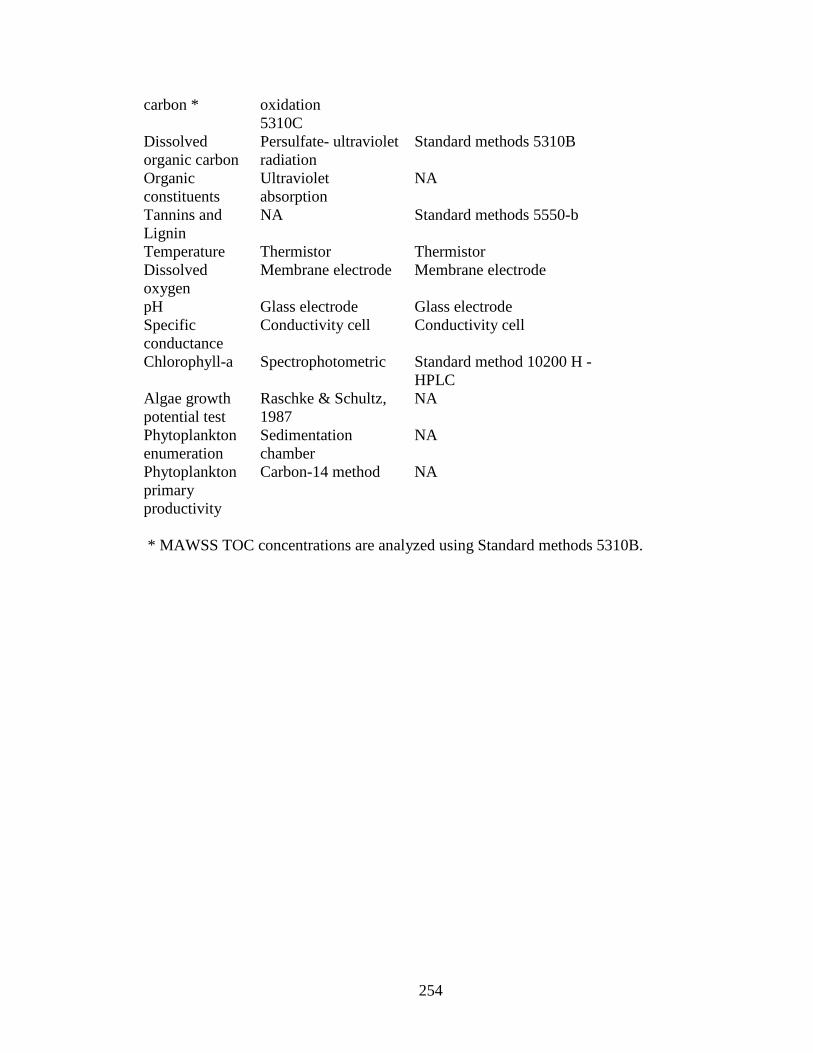
254
carbon * oxidation 5310C
Dissolved organic carbon
Persulfate- ultraviolet radiation
Standard methods 5310B
Organic constituents
Ultraviolet absorption
NA
Tannins and Lignin
NA Standard methods 5550-b
Temperature Thermistor Thermistor Dissolved oxygen
Membrane electrode Membrane electrode
pH Glass electrode Glass electrode Specific conductance
Conductivity cell Conductivity cell
Chlorophyll-a Spectrophotometric Standard method 10200 H - HPLC
Algae growth potential test
Raschke & Schultz, 1987
NA
Phytoplankton enumeration
Sedimentation chamber
NA
Phytoplankton primary productivity
Carbon-14 method NA
* MAWSS TOC concentrations are analyzed using Standard methods 5310B.

255
Appendix N. Calibration and validation profile plots of measured and simulated temperature and dissolved oxygen. Temperature and dissolved oxygen are reported from Hamilton Creek channel near the MAWSS drinking water intake (cell 27, 18) (Figure T-1). Cell 27, 18 was selected for temperature and dissolved oxygen profile reporting because it has a depth similar to measured profiles. Cell 34,18, which is adjacent to the drinking water intake, has a bottom elevation of 29.5 meters above mean sea level. The average water surface elevation is 33.5 meters above mean sea level and the typical depth at cell 34,18 is 4 meters. This corresponds with bathymetry measurements taken across the drinking water intake embayment (Figure T-2, site LHAM), wherein the bottom elevation is slightly greater than 4 meters, except for a deeper center channel with a depth of 8 meters (Figure T-3). Temperature and dissolved oxygen profiles were collected by USGS and AU in the deepest part of the embayment. In order to compare measured and simulated temperature and dissolved oxygen values of a similar depth, simulated temperature and dissolved oxygen from cell 27,18 are used. Cell 27,18 is the cell nearest the drinking water intake with a typical depth of 8 meters.
Figure N-1. Converse Reservoir simulation grid showing cell 34,18, near the drinking water intake, and cell 27,18, the nearest cell with a depth similar to the dredged channel near the drinking water intake.

256
Figure N-2. Converse lake sampling site showing transect LHAM, which depicts the path of the bathymetry measurement reported in Figure N-3. (Gill et al., 2005).
Intake Bathymetry (0 Depth = 33.5 m Gage Height)
0
2
4
6
8
100 50 100 150 200 250 300 350
Bath
ymet
ry (m
eter
s)
Figure N-3. Intake bathymetry measured across the drinking water intake embayment by USGS. Measured and simulated dissolved oxygen and temperature generally correspond well. Summer measured anoxic conditions are not as visible in the simulated (solid) dissolved oxygen profiles, indicating that the model dissolved oxygen in the reservoir hypolimnion

257
is not decreasing as much as the measured bottom dissolved oxygen. This difference between measured and simulated bottom dissolved oxygen is generally evident June to August. Calibration profile plots of simulated (solid) and observed temperature (ºC) and dissolved oxygen concentration (mg L-1).
Feb 2001
0
1
2
3
4
5
6
7
0 10 20 30
May 2001
0
1
23
4
5
67
8
0 10 20 30
July 2001
0
1
23
4
5
67
8
0 20
Sep 2001
0
1
23
4
5
67
8
0 10 20 30
Apr 2002
0
1
23
4
5
67
8
0 10 20 30
8 May 2002
0
1
23
4
5
67
8
0 10 20 30

258
29 May 2002
0
1
23
4
5
67
8
0 10 20 30
Jun 2002
0
1
23
4
5
67
8
0 10 20 30
8 Jul 2002
0
1
23
4
5
67
8
0 10 20 30
31 Jul 2002
0
1
23
4
5
67
8
0 10 20 30
Aug 2002
0
1
23
4
5
67
8
0 10 20 30
10 Sep 2002
0
1
23
4
5
67
8
0 10 20 30
24 Sep 2002
0123456789
0 10 20 30
Apr 2003
0
1
23
4
5
67
8
0 10 20 30
May 2003
0
1
23
4
5
67
8
0 10 20 30

259
4 Jun 2003
0
1
23
4
5
67
8
0 10 20 30
16 Jun 2003
0
1
23
4
5
67
8
0 10 20 30
Jul 2003
0
1
23
4
5
67
8
0 10 20 30
Aug 2003
0
1
23
4
5
67
8
0 10 20 30
Nov 2003
0
1
23
4
5
67
8
0 10 20 30
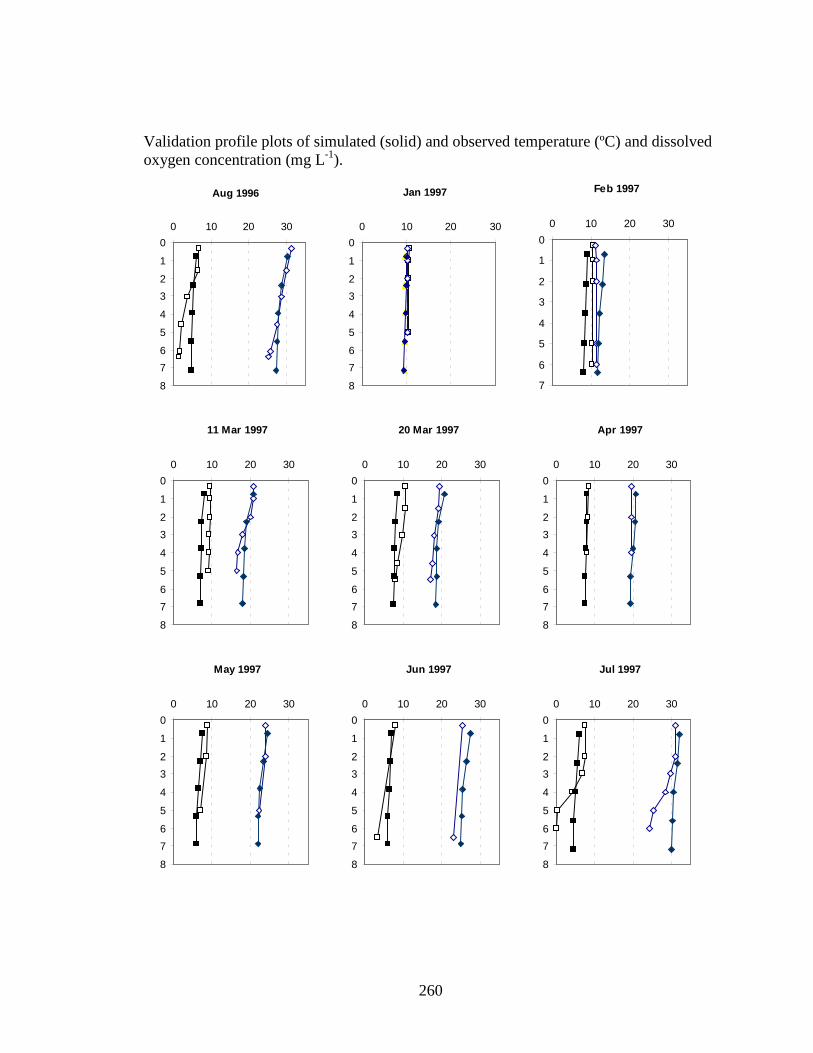
260
Validation profile plots of simulated (solid) and observed temperature (ºC) and dissolved oxygen concentration (mg L-1).
Aug 1996
0
1
23
4
5
67
8
0 10 20 30
Jan 1997
0
1
23
4
5
67
8
0 10 20 30
Feb 1997
0
1
2
3
4
5
6
7
0 10 20 30
11 Mar 1997
0
1
23
4
5
67
8
0 10 20 30
20 Mar 1997
0
1
23
4
5
67
8
0 10 20 30
Apr 1997
0
1
23
4
5
67
8
0 10 20 30
May 1997
0
1
23
4
5
67
8
0 10 20 30
Jun 1997
0
1
23
4
5
67
8
0 10 20 30
Jul 1997
0
1
23
4
5
67
8
0 10 20 30

261
Aug 1997
0
1
23
4
5
67
8
0 10 20 30
Sep 1997
0
1
23
4
5
67
8
0 10 20 30
Oct 1997
0
1
23
4
5
67
8
0 10 20 30
Nov 1997
0
1
23
4
5
67
8
0 10 20 30
Dec 1997
0
1
2
3
45
6
7
8
0 10 20 30

262
Appendix O. Data distribution of TN, TP and TOC data near the MAWSS drinking water intake (34,18). Histograms and quantile-quantile (Q-Q) normal plots of residuals (observed value – mean of observations) are provided below, along with skewness coefficients, to evaluate the assumption of a normal data distribution for TN, TP and TOC near the MAWSS drinking water intake. Data used in the analyses are from 1 Jan 1992 to 31 Dec 1999 and 1 Aug 2002 to 30 April 2005 (n=4,292). A total of 4,292 daily simulated values for each scenario are used in the graphs and analyses. In general, the distributions are slightly right-skewed, meaning that the right tail is long relative to the left tail of the distribution. The plots indicate that the data are not normally distributed and nonparametric methods for data analysis are used. The skewness for a normally distributed data set is zero. TN skewness ranges from 0.61 to 0.89, indicating that data are not normally distributed. TP skewness ranges from 0.4 to 1.64. Base TP values have a greater skewness than future for TOC. TOC future scenario data appear to have a distribution closer to normal than base scenarios. TOC skewness ranges from 0.44 to 1.28. Table O-1. Skewness coefficients based upon residuals (n=4,292) TN TP TOC Base 0.61 1.64 1.28 Future 0.87 1.02 0.51

263
-0.12 -0.08 -0.05 -0.01 0.03 0.07 0.11 0.15 0.19 0.23 0.27Base92 TN residuals
0
200
400
600
800
1000
Histogram of base TN residuals
-0.20 -0.12 -0.04 0.04 0.12 0.20 0.28 0.36 0.44 0.52 0.60Future TN residuals
0
400
800
1200
Histogram of future TN residuals
-0.006 -0.001 0.003 0.007 0.011 0.015 0.020 0.024 0.028 0.032 0.037Base92 TP residuals
0
500
1000
1500
2000
Histogram of base TP residuals
-0.0079 0.0013 0.0106 0.0198 0.0291 0.0383Future TP residuals
0
500
1000
1500
2000
Histogram of future TP residuals
-1.02 -0.52 -0.01 0.49 1.00 1.50 2.01 2.51 3.02 3.52 4.03Base92 TOC residuals
0
500
1000
1500
Histogram of pre-urban92 TOC residuals
-1.45 -0.85 -0.25 0.36 0.96 1.56 2.16 2.76 3.36 3.97 4.57Future92 TOC residuals
0
500
1000
1500
Histogram of future TOC residuals

264
Q-Q Normal Plots
-4 -2 0 2 4Normal Distribution
-0.2
-0.1
0.0
0.1
0.2
0.3
-4 -2 0 2 4Normal Distribution
-0.2
0.0
0.2
0.4
0.6
TN fu
ture
92
Base 1992 MRLC TN residuals Future TN residuals
-4 -2 0 2 4Normal Distribution
-0.01
0.00
0.01
0.02
0.03
-4 -2 0 2 4
Normal Distribution
-0.01
0.00
0.01
0.02
0.03
0.04
TP fu
ture
92
Base 1992 MRLC TP residuals Future TP residuals
-4 -2 0 2 4Normal Distribution
-2
0
2
4
-4 -2 0 2 4
Normal Distribution
-2
0
2
4
TOC
futu
re92
Base 1992 MRLC TOC residuals Future TOC residuals