VALUING COMPANIES BY CASH FLOW DISCOUNTING: …

IESE Business School-University of Navarra - 1

VALUING COMPANIES BY CASH FLOW DISCOUNTING: FUNDAMENTAL RELATIONSHIPS AND UNNECESSARY COMPLICATIONS

Pablo Fernández

IESE Business School – University of Navarra Av. Pearson, 21 – 08034 Barcelona, Spain. Phone: (+34) 93 253 42 00 Fax: (+34) 93 253 43 43 Camino del Cerro del Águila, 3 (Ctra. de Castilla, km 5,180) – 28023 Madrid, Spain. Phone: (+34) 91 357 08 09 Fax: (+34) 91 357 29 13 Copyright © 2013 IESE Business School.

Working Paper

WP-1062-E

February 2013

IESE Business School-University of Navarra

VALUING COMPANIES BY CASH FLOW DISCOUNTING: FUNDAMENTAL RELATIONSHIPS AND UNNECESSARY

COMPLICATIONS

Pablo Fernández1

Abstract

Company valuation using discounted cash flows is based on the valuation of government bonds: it consists of applying the procedure used to value government bonds to the debt and shares of a company. This is easy to understand (sections 1, 2 and 3).

But company valuations are often complicated by “additions” (formulae, concepts, theories…) to complicate its understanding (see sections 4 to 15) and to provide a more “scientific,” “serious,” “intriguing,” “impenetrable”… appearance. Among the most commonly used “additions” are: WACC, beta (), market risk premium, beta unlevered, value of tax shields…. Most of these “additions” are unnecessary complications and are the source of many errors (section 16).

JEL Classification: G12, G31, M21

Keywords: valuation, discounted cash flow, required equity premium, WACC, expected equity premium, beta, VTS.

1 Professor, Financial Management, PricewaterhouseCoopers Chair of Finance, IESE

IESE Business School-University of Navarra

VALUING COMPANIES BY CASH FLOW DISCOUNTING: FUNDAMENTAL RELATIONSHIPS AND UNNECESSARY

COMPLICATIONS

Contents 1 Valuation of Government Bonds 2 Extension of the Valuation of Government Bonds to the Valuation of Companies 2.1 Valuation of the Debt 2.2 Valuation of the Shares 3 Example 4 First Complication: Beta () and Market Risk Premium 5 Second Complication: The Free Cash Flow and the WACC 6 Third Complication: The Capital Cash Flow and the WACCBT 7 Fourth Complication: The Present Value of the Tax Savings Due to Interest Payments 8 Fifth Complication: The Unlevered Company, Ku and Vu 9 Sixth Complication: Different Theories About the VTS 10 Several Relationships Between the Unlevered Beta (U) and the Levered Beta (L) 11 More Relationships Between the Unlevered Beta and the Levered Beta 12 Mixing Accounting Data With the Valuation: The Economic Profit 13 Another Mix of Accounting Data With the Valuation: The EVA (Economic Value Added) 14 To Maintain That the Levered Beta May Be Calculated With a Regression of Historical Data 15 To Maintain That “the Market” Has “an MRP” and That It Is Possible to Estimate It 16 Some Errors Due to Using Unnecessary Complications

Exhibit 1. Concepts and Main Equations Exhibit 2. Main Results of the Example Exhibit 3. Some Articles About the Value of Tax Shields (VTS)

2 - IESE Business School-University of Navarra

1. Valuation of Government Bonds The valuation of companies using discounted cash flows is an extension of the valuation of government bonds. A government bond is a piece of paper1 that details the amount in U.S. dollars that its owner will receive and the dates on which the amounts will be received. The amounts promised in the government bond are called cash flows and are the money (cash) that will go from the government to the pocket of the owner of the bond on the specified days.

The value of a government bond (VGB) is the present value of the cash flows promised in the bond (CFgb) using the so called “risk-free rate” (RF):

Value of a government bond = VGB = PV (CFgb; RF) (1)

The risk-free rate (RF) is the required return on government bonds.

2. Extension of the Valuation of Government Bonds to the Valuation of Companies The valuation of companies deals with the valuation of the financial debt and with the valuation of the shares (equity). We apply Equation (1) to the valuation of debt and to the valuation of shares.

2.1 Valuation of the Debt

The debt of the company is: several pieces of paper2 that include the amounts that their owners will receive on specified dates. The amounts promised by the debt are called debt cash flows (CFd), and are interest payments and repayments of debt (N).3

CFd = Interest + N (2)

As the debt cash flows (CFd) promised by a company are usually riskier4 than the cash flows promised by the government bonds (CFgb), the required return to debt (Kd) is usually higher than the risk-free rate (RF).

Required return to debt = Kd = RF + RPd (debt risk premium) (3)

1 It can also be an electronic record. In that case we should say “as it would be” a piece of paper. 2 If it is bank debt, the owners of the papers are banks. If the debts are bonds, notes… the owners of the papers are the persons, the companies and the financial institutions that bought them. 3 If the company does not repay debt (N) but increases its debt (N), Equation (2) would be CFd = Interest - N. 4 The risk of the debt is the probability that the company will not pay some of the promised cash flows. Risk-free debt means that we assume that the company will pay all promised cash flows for sure.


The debt risk premium (RPd) depends on the perceived risk on the debt (expectations of getting less money than the promised debt cash flows) by every investor. Applying Equation (1) to the debt of the company, we get:

Value of debt = D = PV (CFd; Kd) (4)

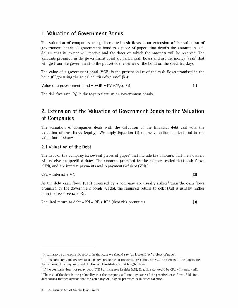
Cash Working capital Debt cash flow (CFd): money (cash) that goes from

the cash of the company to the pockets of bondholders

requirements Debt (N) (WCR) Bank debt, bonds…

Net fixed Book value of equity

(Ebv) Equity cash flow (ECF): money (cash) that goes from the cash of the company to the pockets of shareholders assets (NFA) Shares

2.2 Valuation of the Shares

A share of a company is a piece of paper that, contrary to debt, has neither dates nor amounts that its owner, the shareholder, will receive. We need, first, to estimate the expected cash flows for the owners of the shares in the following years, named equity cash flows (ECF). A usual way of estimating the ECF is to start with the expected balance sheets and P&Ls. Equation (5) is the basic accounting identity: assets are equal to liabilities and equity:

Cash + WCR + NFA = N + Ebv (5)

Equation (6) is the annual change of Equation (5). The increase of the cash of the company before giving anything to the shareholders will be divided between the equity cash flow (ECF) and the increase of cash (Cash) decided by the managers:

ECF + Cash + WCR + NFA = N + Ebv (6)

If the increase of the book value of equity (Ebv) is due only to the profit after tax (PAT) of the year, then:5

ECF = PAT - WCR - NFA + N - Cash (7)

As the expected equity cash flows (ECF) are riskier than the cash flows promised by government bonds (CFgb) and also riskier than the cash flows promised by the debt of the company (CFd), the required return to equity (shares) (Ke) is higher than the risk-free rate (RF) and also higher than the required return to debt (Kd):

Ke = RF + RPs (share risk premium) (8)

5 As NFA = GFA (gross fixed assets) - depreciation, equation (7) can be written: ECF = PAT + depreciation - NOF - GFA + N - Cash


The so-called share risk premium (RPs) depends on the estimated (expected) risk of the expected equity cash flows (ECF). Obviously, this parameter depends on the expectations of each investor. Applying Equation (1) to the equity (the shares of the company), we get:

Value of the shares (equity value) = E = PV (ECF; Ke) (9)

With Equations (2) to (9) we can value any company.

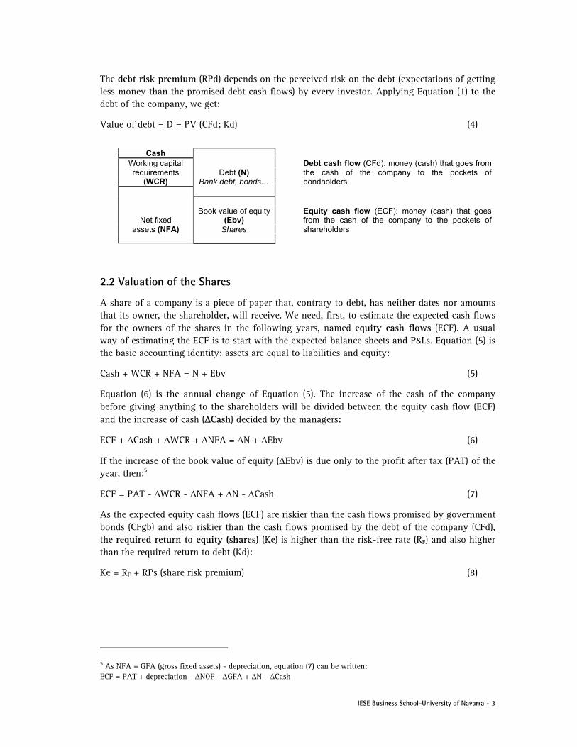
3. Example The expected balance sheets and P&Ls of company AAA are the following (amounts in $ millions):

Balance Sheet Year 0 1 2 …g = 2% P&L 1 2 …g = 2%

Cash 50 51 52.02 Sales 2400 2448.0

WCR 450 459 468.18 Cost of sales 1200 1224.0

Gross fixed assets (GFA) 1500 1680 1863.60 Other expenses 810 826.2

- cumul. depreciation 150 303.00 Depreciation 150 153.0

Net fixed assets (NFA) 1500 1530 1560.60 Interest 60 61.2

TOTAL NET ASSETS 2000 2040 2080.80 PBT (Profit before taxes) 180 183.6

Taxes (25%) 45 45.9

Debt (N) 1000 1020 1040.40 PAT (Profit after taxes) 135 137.7

Book value of equity (Ebv) 1000 1020 1040.00

TOTAL Liabilities and Equity 2000 2040 2080.80

The managers of AAA expect that the balance sheet (cash, WCR, NFA, N and Ebv) and the P&L will grow annually 2%.

The interest rate of the debt (r) is 6%. The interest to be paid in year one is $60 = N r = 1000 x 6%. The amount of debt is expected to increase in $20 million in year one. Then, in year one:

(2) CFd = Interest - N = 60 – 20 = 40

The risk-free rate (RF) of the long-term government bonds (10 years) is 4%. The financial manager of AAA considers that an RPd (debt risk premium) of 2% is appropriate for the debt of AAA. Then:

(3) Kd = RF + RPd (debt risk premium) = 4% + 2% = 6%

As the required return to debt (Kd = 6%) is equal to the interest rate paid (r = 6%), D = N = 1000. We can calculate D using Equation (4):

Value of debt = D = PV (CFd; Kd) =

In company AAA the increase of the book value of equity (�Ebv) is due only to the profit after tax of the year. Applying Equation (7) to year one:

(7) ECF = PAT - WCR - NFA + N - Cash = 115 = 135 - 9 - 30 + 20 - 1

100002.006.0

40...

06.1

)02.1(40

06.1

)02.1(40

06.1

403

2

2


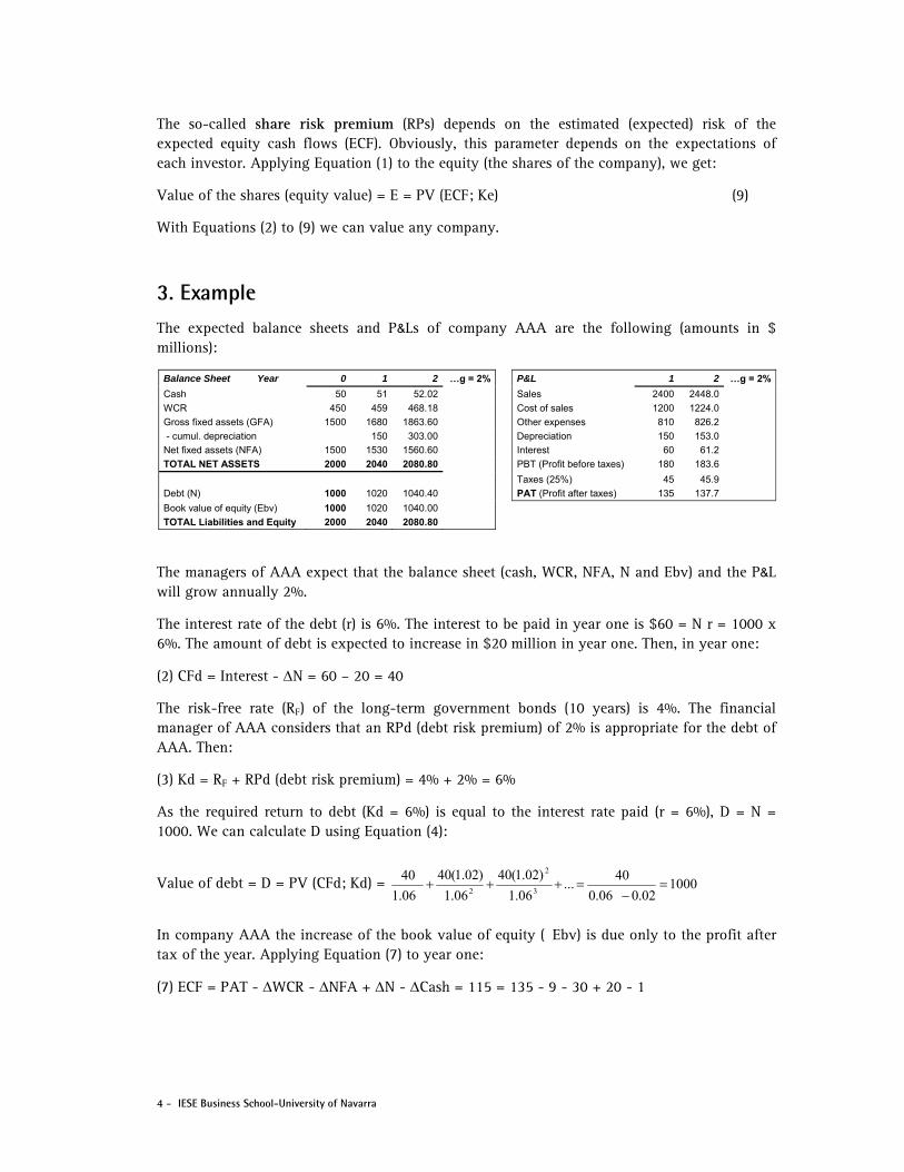
The next table applies Equation (7) to years one and two.

1 2

PAT (profit after tax) 135 137.7

+ Depreciation 150 153.00 + ∆ Debt 20 20.40 - ∆ Cash -1 -1.02 - ∆ WCR -9 -9.18 - Investments (∆GFA) -180 -183.60 ECF (equity cash flow) 115 117.30 … grows 2% annually

The financial manager of AAA considers that 5% is an appropriate share risk premium (RPs) for the equity (shares) of AAA. Then, the required return to equity (Ke) is:

(8) Ke = RF + RPs = 4% + 5% = 9%

Now, we can use Equation (9) to calculate the value of the shares or equity value (E) of AAA:

(9) E = PV (ECF; Ke) =

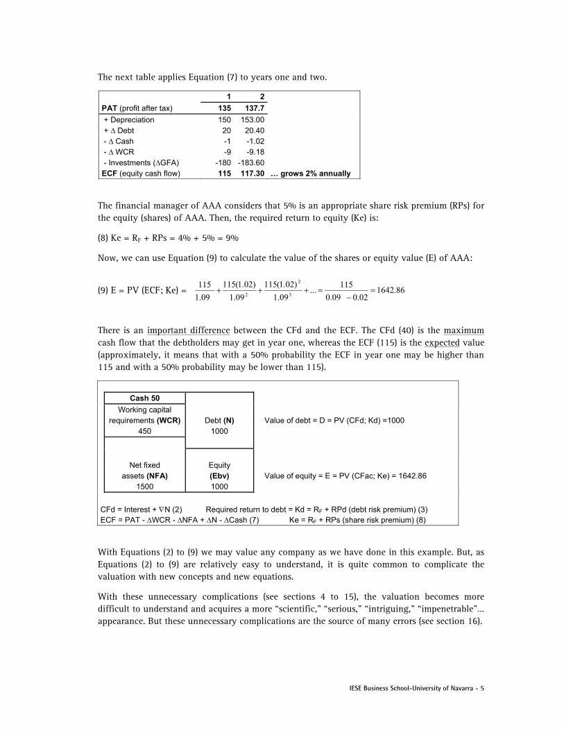
There is an important difference between the CFd and the ECF. The CFd (40) is the maximum cash flow that the debtholders may get in year one, whereas the ECF (115) is the expected value (approximately, it means that with a 50% probability the ECF in year one may be higher than 115 and with a 50% probability may be lower than 115).

Cash 50

Working capital requirements (WCR) Debt (N) Value of debt = D = PV (CFd; Kd) =1000 450 1000

Net fixed Equity assets (NFA) (Ebv) Value of equity = E = PV (CFac; Ke) = 1642.86 1500 1000

CFd = Interest + N (2) Required return to debt = Kd = RF + RPd (debt risk premium) (3) ECF = PAT - WCR - NFA + N - Cash (7) Ke = RF + RPs (share risk premium) (8)

With Equations (2) to (9) we may value any company as we have done in this example. But, as Equations (2) to (9) are relatively easy to understand, it is quite common to complicate the valuation with new concepts and new equations.

With these unnecessary complications (see sections 4 to 15), the valuation becomes more difficult to understand and acquires a more “scientific,” “serious,” “intriguing,” “impenetrable”… appearance. But these unnecessary complications are the source of many errors (see section 16).

86.164202.009.0

115...

09.1

)02.1(115

09.1

)02.1(115

09.1

1153

2

2


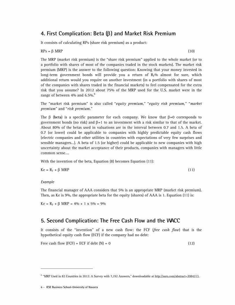
4. First Complication: Beta () and Market Risk Premium It consists of calculating RPs (share risk premium) as a product:

RPs = MRP (10)

The MRP (market risk premium) is the “share risk premium” applied to the whole market (or to a portfolio with shares of most of the companies traded in the stock markets). The market risk premium (MRP) is the answer to the following question: Knowing that your money invested in long-term government bonds will provide you a return of RF% almost for sure, which additional return would you require on another investment (in a portfolio with shares of most of the companies with shares traded in the financial markets) to feel compensated for the extra risk that you assume? In 2012 about 75% of the MRP used for the U.S. market were in the range of between 4% and 6.5%.6

The “market risk premium” is also called “equity premium,” “equity risk premium,” “market premium” and “risk premium.”

The (beta) is a specific parameter for each company. We know that =0 corresponds to government bonds (no risk) and =1 to an investment with a risk similar to that of the market. About 80% of the betas used in valuations are in the interval between 0.7 and 1.5. A beta of 0.7 (or lower) could be applicable to companies with highly predictable equity cash flows (electric companies and other utilities in countries with expectations of very few surprises and sensible managers…). A beta of 1.5 (or higher) could be applicable to new companies with high uncertainty about the market acceptance of their products, companies with managers with little common sense….

With the invention of the beta, Equation (8) becomes Equation (11):

Ke = RF + MRP (11)

Example

The financial manager of AAA considers that 5% is an appropriate MRP (market risk premium). Then, as Ke is 9%, the appropriate beta for the equity (shares) of AAA is 1. Equation (11) is:

Ke = RF + MRP = 4% + 1 x 5% = 9%

5. Second Complication: The Free Cash Flow and the WACC It consists of the “invention” of a new cash flow: the FCF (free cash flow) that is the hypothetical equity cash flow (ECF) if the company had no debt:

Free cash flow (FCF) = ECF if debt (N) = 0 (12)

6 “MRP Used in 82 Countries in 2012: A Survey with 7,192 Answers,” downloadable at http://ssrn.com/abstract=2084213.


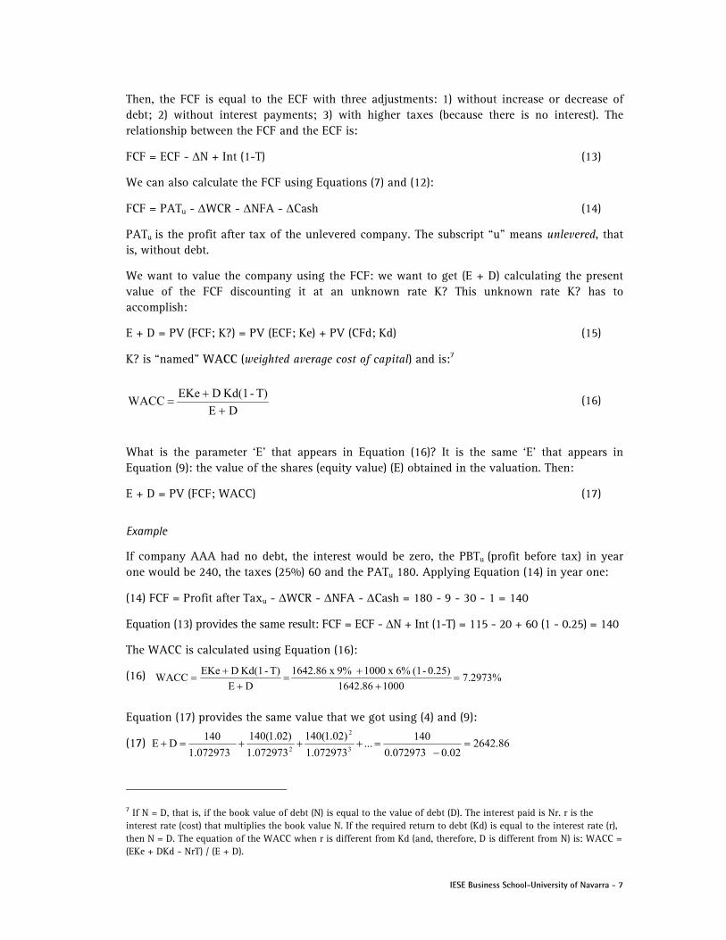
Then, the FCF is equal to the ECF with three adjustments: 1) without increase or decrease of debt; 2) without interest payments; 3) with higher taxes (because there is no interest). The relationship between the FCF and the ECF is:

FCF = ECF - N + Int (1-T) (13)

We can also calculate the FCF using Equations (7) and (12):

FCF = PATu - WCR - NFA - Cash (14)

PATu is the profit after tax of the unlevered company. The subscript “u” means unlevered, that is, without debt.

We want to value the company using the FCF: we want to get (E + D) calculating the present value of the FCF discounting it at an unknown rate K? This unknown rate K? has to accomplish:

E + D = PV (FCF; K?) = PV (ECF; Ke) + PV (CFd; Kd) (15)

K? is “named” WACC (weighted average cost of capital) and is:7

(16)

What is the parameter ‘E’ that appears in Equation (16)? It is the same ‘E’ that appears in Equation (9): the value of the shares (equity value) (E) obtained in the valuation. Then:

E + D = PV (FCF; WACC) (17)

Example

If company AAA had no debt, the interest would be zero, the PBTu (profit before tax) in year one would be 240, the taxes (25%) 60 and the PATu 180. Applying Equation (14) in year one:

(14) FCF = Profit after Taxu - WCR - NFA - Cash = 180 - 9 - 30 - 1 = 140

Equation (13) provides the same result: FCF = ECF - N + Int (1-T) = 115 - 20 + 60 (1 - 0.25) = 140

The WACC is calculated using Equation (16):

(16)

Equation (17) provides the same value that we got using (4) and (9):

(17)

7 If N = D, that is, if the book value of debt (N) is equal to the value of debt (D). The interest paid is Nr. r is the interest rate (cost) that multiplies the book value N. If the required return to debt (Kd) is equal to the interest rate (r), then N = D. The equation of the WACC when r is different from Kd (and, therefore, D is different from N) is: WACC = (EKe + DKd - NrT) / (E + D).

86.264202.0072973.0

140...

072973.1

)02.1(140

072973.1

)02.1(140

072973.1

140DE

3

2

2

7.2973% 10001642.86

0.25)-(1 6% x 1000 9% x 1642.86

DE

T) - Kd(1 D EKeWACC

DE

T) - Kd(1 D EKeWACC


6. Third Complication: The Capital Cash Flow and the WACCBT

It consists of the “invention” of a new cash flow: the CCF (capital cash flow), which is the sum of the equity cash flow (ECF) and the debt cash flow (CFd):

CCF = ECF + CFd (18)

The relationship between the CCF and the FCF is:

CCF = FCF + Int T (19)

We want to value the company using the CCF: we want to get (E + D) calculating the present value of the CCF discounting it at an unknown rate K? This unknown rate K? has to accomplish:

E + D = PV (CCF; K?) = PV (ECF; Ke) + PV (CFd; Kd) = PV (FCF; WACC) (20)

K? is “named” WACCBT (weighted average cost of capital before taxes) and is:

(21)

Then,

E + D = PV (CCF; WACCBT) (22)

Example

In company AAA, the CCF (capital cash flow) of year one is: (18) CCF = ECF + CFd = 115 + 40 =155

We could also use Equation (19): CCF = FCF + Int T = 140 + 60 x 0.25 = 155

(21)

And (22) E + D = PV (CCF; WACCBT) = 155 / (0.786487 - 0.02) = 2642.858

7. Fourth Complication: The Present Value of the Tax Savings Due to Interest Payments (VTS) We can calculate the present value of tax savings arising from the use of debt (tax shields). It is usually named value of tax shields (VTS). If all interest paid is tax-deductible, the tax shield of a year is the product of the interest paid (N r) times the tax rate (T). If we assume that the risk of the tax shields is the same as the risk of the debt:

VTS = PV (N r T; Kd) (23)

8 We have an error of one cent because, to simplify, we calculate the WACCBT using only two decimal figures of E: 1642.86; instead of 1642.85714.

%86487.7 000186.6421

6% x 1000 9% x 1642.86

DE

Kd D EKeWACCBT

DE

Kd D EKeWACC BT


Example

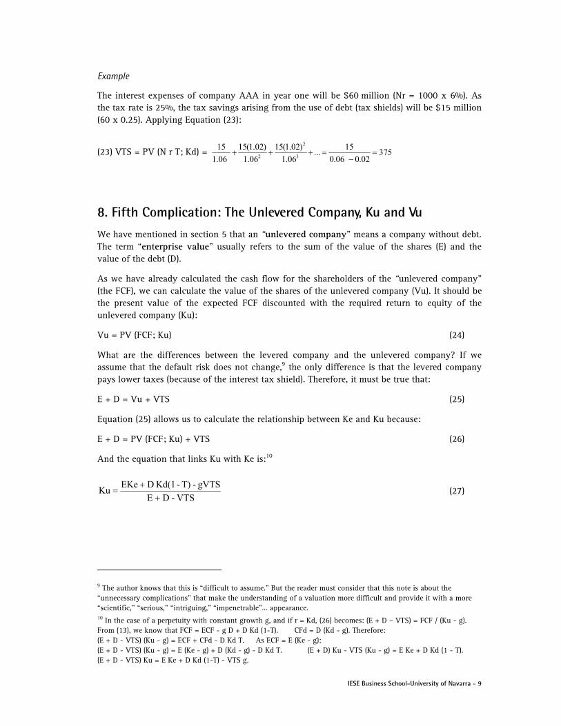
The interest expenses of company AAA in year one will be $60 million (Nr = 1000 x 6%). As the tax rate is 25%, the tax savings arising from the use of debt (tax shields) will be $15 million (60 x 0.25). Applying Equation (23):

(23) VTS = PV (N r T; Kd) =

8. Fifth Complication: The Unlevered Company, Ku and Vu

We have mentioned in section 5 that an “unlevered company” means a company without debt. The term “enterprise value” usually refers to the sum of the value of the shares (E) and the value of the debt (D).

As we have already calculated the cash flow for the shareholders of the “unlevered company” (the FCF), we can calculate the value of the shares of the unlevered company (Vu). It should be the present value of the expected FCF discounted with the required return to equity of the unlevered company (Ku):

Vu = PV (FCF; Ku) (24)

What are the differences between the levered company and the unlevered company? If we assume that the default risk does not change,9 the only difference is that the levered company pays lower taxes (because of the interest tax shield). Therefore, it must be true that:

E + D = Vu + VTS (25)

Equation (25) allows us to calculate the relationship between Ke and Ku because:

E + D = PV (FCF; Ku) + VTS (26)

And the equation that links Ku with Ke is:10

(27)

9 The author knows that this is “difficult to assume.” But the reader must consider that this note is about the “unnecessary complications” that make the understanding of a valuation more difficult and provide it with a more “scientific,” “serious,” “intriguing,” “impenetrable”… appearance. 10 In the case of a perpetuity with constant growth g, and if r = Kd, (26) becomes: (E + D – VTS) = FCF / (Ku - g). From (13), we know that FCF = ECF - g D + D Kd (1-T). CFd = D (Kd - g). Therefore: (E + D - VTS) (Ku - g) = ECF + CFd - D Kd T. As ECF = E (Ke - g): (E + D - VTS) (Ku - g) = E (Ke - g) + D (Kd - g) - D Kd T. (E + D) Ku - VTS (Ku - g) = E Ke + D Kd (1 - T). (E + D - VTS) Ku = E Ke + D Kd (1-T) - VTS g.

37502.006.0

15...

06.1

)02.1(15

06.1

)02.1(15

06.1

153

2

2

VTS-DE

gVTS-T)-Kd(1 D EKeKu


Example

(27)

(24) Vu = 140 /(0.0817323 - 0.02) = 2267.86

(25) 2267.86 + 375 = 1642.86 + 1000

VTS 375 VTS = PV (N r T; Kd) D = PV (CFd; Kd) Debt (D) 1000.00 Vu Vu = PV (FCF; Ku) Shares 2267.86 E = PV (ECF; Ke) E 1642.86

E + D = PV (FCF; WACC) = PV (CCF; WACCBT) = Vu + VTS

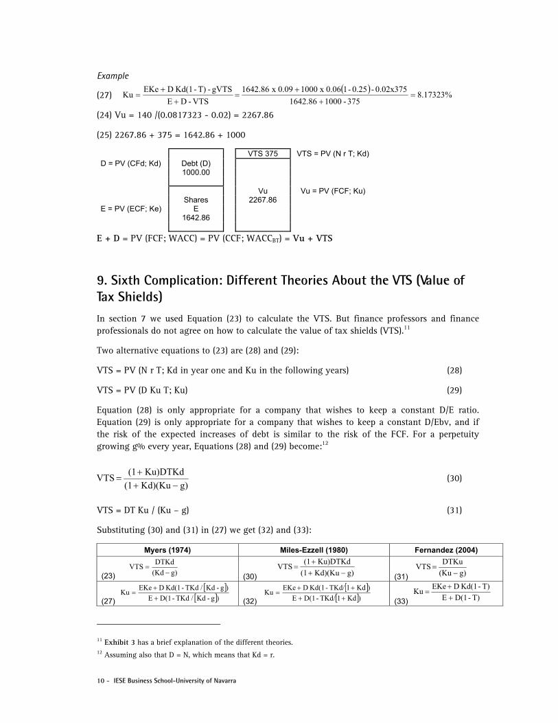
9. Sixth Complication: Different Theories About the VTS (Value of Tax Shields) In section 7 we used Equation (23) to calculate the VTS. But finance professors and finance professionals do not agree on how to calculate the value of tax shields (VTS).11

Two alternative equations to (23) are (28) and (29):

VTS = PV (N r T; Kd in year one and Ku in the following years) (28)

VTS = PV (D Ku T; Ku) (29)

Equation (28) is only appropriate for a company that wishes to keep a constant D/E ratio. Equation (29) is only appropriate for a company that wishes to keep a constant D/Ebv, and if the risk of the expected increases of debt is similar to the risk of the FCF. For a perpetuity growing g% every year, Equations (28) and (29) become:12

(30)

VTS = DT Ku / (Ku – g) (31)

Substituting (30) and (31) in (27) we get (32) and (33):

Myers (1974) Miles-Ezzell (1980) Fernandez (2004)

(23)

g)(Kd

DTKdVTS

(30)

g)Kd)(Ku(1

Ku)DTKd(1VTS

(31)

g)(Ku

DTKuVTS

(27)

)g-Kd / TKd-D(1E

)g-Kd / TKd-Kd(1 D EKeKu

(32)

)Kd1TKd/-D(1E

)Kd1TKd/-Kd(1 D EKeKu

(33)

T)-D(1E

T)-Kd(1 D EKeKu

11 Exhibit 3 has a brief explanation of the different theories. 12 Assuming also that D = N, which means that Kd = r.

8.17323%

375-10001642.86

0.02x375-0.25-10.06 x 1000 0.09 x 1642.86

VTS-DE


g)Kd)(Ku(1

Ku)DTKd(1VTS


Example

Equation (32) applied to company AAA results in Ku = 7.8749%. Equation (33), Ku = 8.0597%

Equation (30): VTS = 259.84. Equation (31): 332.51. Vu is 2383.02 according to (32) and 2310.35 according to (33)

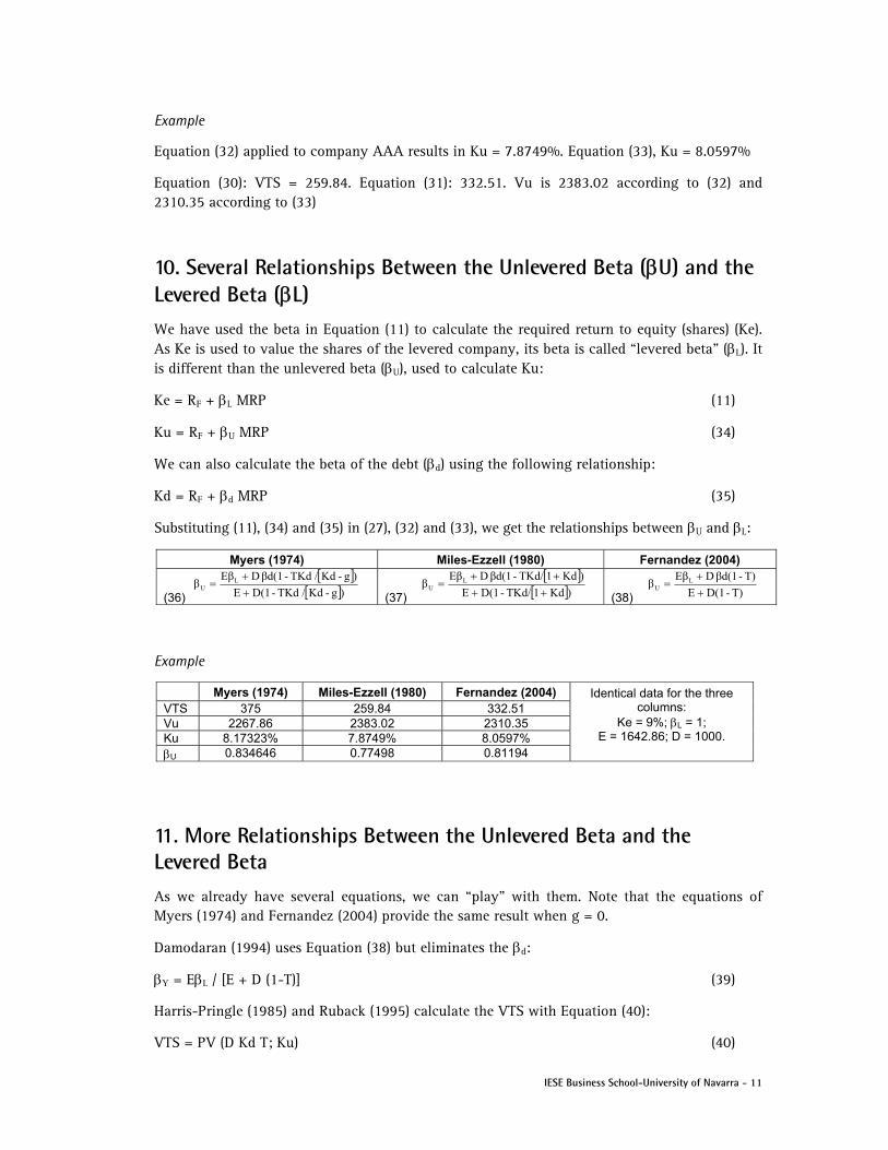
10. Several Relationships Between the Unlevered Beta (U) and the Levered Beta (L) We have used the beta in Equation (11) to calculate the required return to equity (shares) (Ke). As Ke is used to value the shares of the levered company, its beta is called “levered beta” (L). It is different than the unlevered beta (U), used to calculate Ku:

Ke = RF + L MRP (11)

Ku = RF + U MRP (34)

We can also calculate the beta of the debt (d) using the following relationship:

Kd = RF + d MRP (35)

Substituting (11), (34) and (35) in (27), (32) and (33), we get the relationships between U and L:

Myers (1974) Miles-Ezzell (1980) Fernandez (2004)

(36)

)g-Kd /TKd-D(1E

)g-Kd /TKd-βd(1 D Eββ L

U

(37)

)Kd1TKd/-D(1E

)Kd1TKd/-βd(1 D Eββ L

U

(38)

T)-D(1E

T)-βd(1 D Eββ L

U

Example

Myers (1974) Miles-Ezzell (1980) Fernandez (2004) Identical data for the three columns:

Ke = 9%; L = 1; E = 1642.86; D = 1000.

VTS 375 259.84 332.51 Vu 2267.86 2383.02 2310.35 Ku 8.17323% 7.8749% 8.0597% U 0.834646 0.77498 0.81194

11. More Relationships Between the Unlevered Beta and the Levered Beta As we already have several equations, we can “play” with them. Note that the equations of Myers (1974) and Fernandez (2004) provide the same result when g = 0.

Damodaran (1994) uses Equation (38) but eliminates the d:

= EL / [E + D (1-T)] (39)

Harris-Pringle (1985) and Ruback (1995) calculate the VTS with Equation (40):

VTS = PV (D Kd T; Ku) (40)


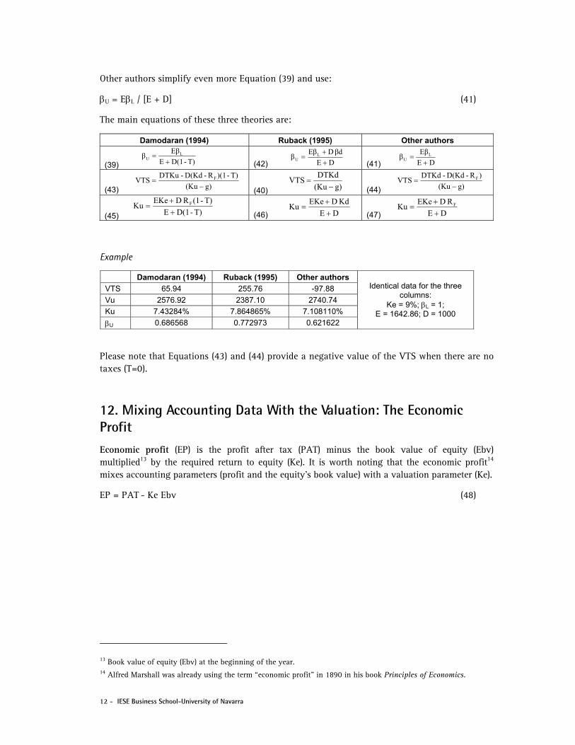
Other authors simplify even more Equation (39) and use:

U = EL / [E + D] (41)

The main equations of these three theories are:

Damodaran (1994) Ruback (1995) Other authors

(39)

T)-D(1E

Eββ L

U

(42)

DE

βd D Eββ L

U

(41)

DE

Eββ L

U

(43)

g)(Ku

T)-)(1R-D(Kd-DTKuVTS F

(40)

g)(Ku

DTKdVTS

(44)

g)(Ku

)R-D(Kd-DTKdVTS F

(45)

T)-D(1E

T)-(1R D EKeKu F

(46)

DE

Kd D EKeKu

(47)

DE

R D EKeKu F

Example

Damodaran (1994) Ruback (1995) Other authors Identical data for the three

columns: Ke = 9%; L = 1;

E = 1642.86; D = 1000

VTS 65.94 255.76 -97.88

Vu 2576.92 2387.10 2740.74

Ku 7.43284% 7.864865% 7.108110%

U 0.686568 0.772973 0.621622

Please note that Equations (43) and (44) provide a negative value of the VTS when there are no taxes (T=0).

12. Mixing Accounting Data With the Valuation: The Economic Profit Economic profit (EP) is the profit after tax (PAT) minus the book value of equity (Ebv) multiplied13 by the required return to equity (Ke). It is worth noting that the economic profit14 mixes accounting parameters (profit and the equity’s book value) with a valuation parameter (Ke).

EP = PAT - Ke Ebv (48)

13 Book value of equity (Ebv) at the beginning of the year. 14 Alfred Marshall was already using the term “economic profit” in 1890 in his book Principles of Economics.


Using the economic profit, we get a new equation to value the shares of the company:15

E = Ebv + PV (PAT – Ke Ebv; Ke) = Ebv + PV (EP; Ke) (49)

Example

(48) EP1 = PAT1 - Ke Ebv0 = 135 - 0.09 x 1000 = 45

(49) E = Ebv + PV (EP; Ke) = 1000 + 45 / (0.09 - 0.02) = 1000 + 642.86 = 1642.86

13. Another Mix of Accounting Data With the Valuation: The EVA (Economic Value Added)

EVA (economic value added) is the term used16 to define:

EVA = NOPAT - (D + Ebv)WACC (50)

NOPAT (net operating profit after taxes) is the profit after tax (PAT) of the company without debt. Sometimes it is also called PATu (as in section 5) and NOPLAT (net operating profit less adjusted taxes).

Using EVA, we get a new equation to value the company:17

E + D = Ebv + D + PV (EVA; WACC) (51)

15 In companies that do not issue shares and have no direct charges to equity, it happens that:

ECF t = PATt - �Ebvt = PATt - (Ebvt - Ebvt-1). As E = PV (ECF; Ke):

Taking into account that Ebv0 / (1+Ke) = Ebv0 – Ke Ebv0 / (1+Ke), the previous equation may be written as:

With some algebra, we get:

16 According to Stern Stewart & Co’s definition. See page 192 of their book The Quest for Value. The EVA Management Guide. 17 In companies that do not issue shares and have no direct charges to equity, it happens that:

FCFt = NOPATt - (∆Ebvt + ∆Dt) As E + D = PV (FCF; WACC):

E + D = [NOPAT1 - (∆Ebv1 + ∆D1)] / (1 + WACC) + [NOPAT2 - (∆Ebv2 + ∆D2)] / (1 + WACC)2 + … = NOPAT1 /(1+WACC) + NOPAT2 /(1 +WACC)2 + … -(Ebv1 + D1 - Ebv0 -D0) /(1+WACC) -(Ebv2 + D2 - Ebv1 - D1) /(1+WACC)2 -…

Given the identity (Ebv0 +D0) / (1+WACC) = Ebv0 +D0 - WACC(Ebv0 +D0) / (1+WACC), the previous equation may be written as:

E + D = NOPAT1 /(1+WACC) + NOPAT2 /(1+WACC)2 +…+(Ebv0 +D0) - (Ebv0 +D0)WACC/ (1+WACC) - (Ebv1 + D1)WACC /(1+WACC)2 -… . ; E + D = Ebv + D + VA [NOPAT - (D + Ebv) WACC; WACC].

...Ke)(1

Ebv Ke

Ke)(1

Ebv Ke

Ke1

Ebv KeFP...

Ke)(1

PAT

Ke1

PATE

32

210

0221

0

...Ke)+(1

Ebv KePAT

Ke+1

Ebv KePATEbvE

21201

00

...Ke)(1

EbvEbvPAT

Ke1

EbvEbvPATE

2122011


Example

(50) EVA = NOPAT - (D + Ebv) WACC =180 – 2000 x 0.072973 = 34.054

(51) E + D = Ebv + D + PV(EVA; WACC) = 2000 + 34.054 / (0.072973 - 0.02) = 2642.86

14. To Maintain That the Levered Beta May Be Calculated With a Regression of Historical Data This new “complication” is a lack of common sense and consists, first, of assuming that “the market” assigns a beta to every company and, second, of maintaining that the levered beta may be calculated with a regression of historical data. According to the followers of this new “complication,” the beta has nothing to do with the expectations of risk, the experience of the valuator… but rather every investor should use the same beta: the calculated beta. You can get that beta running a regression of the past returns of the company against the returns of some market index.

Fernandez (2008)18 shows that it is an enormous error to use calculated betas. First, because it is almost impossible to calculate a meaningful beta because historical betas change dramatically from one day to the next; second, because very often we cannot say with relevant statistical confidence that the beta of one company is smaller or bigger than the beta of another; third, because historical betas do not make much sense in many cases: high-risk companies very often have smaller historical betas than low-risk companies; fourth, because historical betas depend very much on which index we use to calculate them. Industry betas are also unstable: on average, the maximum beta of an industry was 2.7 times its minimum beta in two months.

Some authors and companies publish calculated betas. For example, Damodaran publishes industry betas at http://pages.stern.nyu.edu/~adamodar/New_Home_Page/datafile/Betas.html.

15. To Maintain That “the Market” Has “an MRP” and That It Is Possible to Estimate It This new “complication” consists of assuming that “the market” has an MRP (market risk premium). Then, the MRP would be a parameter “of the market” and not a parameter that is different for different investors.

Fernandez (2010)19 reviews 150 textbooks on corporate finance and valuation written by authors such as Brealey, Myers, Copeland, Damodaran, Merton, Ross, Bruner, Bodie, Penman, Arzac… and finds that their recommendations regarding the equity premium range from 3% to 10%, and that 51 books use different equity premia on various pages. Some confusion arises from not distinguishing among the four concepts that the phrase equity premium designates: the historical, the expected, the implied and the required equity premium (incremental return of a diversified portfolio over the risk-free rate required by an investor).

18 “Are Calculated Betas Worth for Anything?,” downloadable at http://ssrn.com/abstract=504565. 19 “The Equity Premium in 150 Textbooks,” downloadable at http://ssrn.com/abstract=1473225. Of the books, 129 identify expected and required equity premium and 82 identify expected and historical equity premium.


Fernandez, Aguirreamalloa and Corres (2011)20 show that the average market risk premium (MRP) used in 2011 for the United States by professors, analysts and company managers were 5.7%, 5.0% and 5.6% (standard deviation: 1.6%, 1.1% and 2.0%). They also found a great dispersion in the MRP used even if it was justified with the same reference: professors, analysts and companies that cited Ibbotson as their reference used an MRP for the United States of between 2% and 14.5%, and the ones that cited Damodaran as their reference used an MRP of between 2% and 10.8%.

16. Some Errors Due to Using Unnecessary Complications The article “WACC: Definition, Misconceptions and Errors”21 lists seven errors due to not remembering the definition of WACC. Some of the errors are found in many valuations.

The article “110 Common Errors in Company Valuations”22 contains a collection and classification of 110 errors seen in company valuations performed by financial analysts, investment banks and financial consultants. Some of the most common errors are:

1. Errors in the Discount Rate Calculation and Concerning the Riskiness of the Company

Wrong beta used for the valuation.

Using the historical industry beta, or the average of the betas of similar companies, when the result goes against common sense.

Using the historical beta of the company when the result goes against common sense.

Using the wrong formulae for levering and unlevering the beta.

Forgetting the beta of the debt when levering the beta of the shares.

Calculating the beta using not common sense, but strange formulae.

Wrong market risk premium used for the valuation.

Assume that the required market risk premium is equal to the historical equity premium.

Using a risk premium recommended by a book even though it goes against common sense.

Wrong calculation of WACC.

Debt to equity ratio used to calculate the WACC is different than the debt to equity ratio resulting from the valuation.

Calculating the WACC using book values of debt and equity.

Wrong calculation of the value of tax shields (VTS).

20 “US Market Risk Premium Used in 2011 by Professors, Analysts and Companies: A Survey with 5.731 Answers,” downloadable at http://ssrn.com/abstract=1805852. 21 “WACC: definition, misconceptions and errors,” downloadable at http://ssrn.com/abstract=1620871. 22 “110 common errors in company valuations,” downloadable at http://ssrn.com/abstract=1025424.


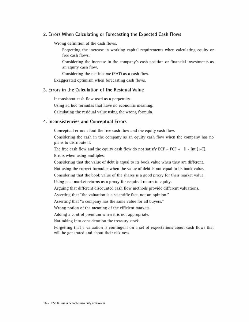
2. Errors When Calculating or Forecasting the Expected Cash Flows

Wrong definition of the cash flows.

Forgetting the increase in working capital requirements when calculating equity or free cash flows.

Considering the increase in the company’s cash position or financial investments as an equity cash flow.

Considering the net income (PAT) as a cash flow.

Exaggerated optimism when forecasting cash flows.

3. Errors in the Calculation of the Residual Value

Inconsistent cash flow used as a perpetuity.

Using ad hoc formulas that have no economic meaning.

Calculating the residual value using the wrong formula.

4. Inconsistencies and Conceptual Errors

Conceptual errors about the free cash flow and the equity cash flow.

Considering the cash in the company as an equity cash flow when the company has no plans to distribute it.

The free cash flow and the equity cash flow do not satisfy ECF = FCF + �D - Int (1-T).

Errors when using multiples.

Considering that the value of debt is equal to its book value when they are different.

Not using the correct formulae when the value of debt is not equal to its book value.

Considering that the book value of the shares is a good proxy for their market value.

Using past market returns as a proxy for required return to equity.

Arguing that different discounted cash flow methods provide different valuations.

Asserting that “the valuation is a scientific fact, not an opinion.”

Asserting that “a company has the same value for all buyers.”

Wrong notion of the meaning of the efficient markets.

Adding a control premium when it is not appropriate.

Not taking into consideration the treasury stock.

Forgetting that a valuation is contingent on a set of expectations about cash flows that will be generated and about their riskiness.


Exhibit 1 Concepts and Main Equations

Cash flows promised by the government bonds (CFgb) Risk-free rate (RF) = required return to government bonds

Value of a government bond = VGB = PV (CFgb; RF) (1)

Debt cash flows (CFd) Repayments of debt (N) Required return to debt (Kd)

CFd = Interest + N (2)

Required return to debt = Kd = RF + RPd (debt risk premium) (3)

Value of debt = D = PV (CFd; Kd) (4)

If the increase of the book value of equity (Ebv) is only due to the profit after tax (PAT) of the year:

ECF = PAT - WCR - NFA + N - Cash (7)

Required return to equity (shares) (Ke) = RF + RPs (share risk premium) (8)

Value of the shares (equity value) = E = PV (ECF; Ke) (9)

RPs (share risk premium) = MRP (market risk premium) (10)

Ke = RF + MRP (11)

Free cash flow (FCF) = ECF if debt (N) = 0 FCF = ECF - N + Int (1-T) (12), (13)

(16)

E + D = PV (FCF; WACC) (17)

Capital cash flow (CCF) = ECF + CFd = FCF + Int T (18), (21)

E + D = PV (CCF; WACCBT) (22)

VTS (value of tax shields) = PV (N r T; Kd) (23)

Value of the shares of the unlevered company (Vu). Required return to equity of the unlevered company (Ku).

Vu = PV (FCF; Ku) E + D = Vu + VTS (24), (25)

(27)

Ku = RF + U MRP. Kd = RF + d MRP (34), (35)

DE

T) - Kd(1 D EKeWACC

DE

Kd D EKeWACCBT

VTS-DE



Exhibit 1 (continued)

Author VTS Ku �u

Myers (1974)

(23)

g)(Kd

DTKdVTS

(27)

)g-Kd / TKd-D(1E

)g-Kd / TKd-Kd(1 D EKe

(36)

)g-KdTKd-D(1E

)g-KdTKd-βd(1 D EβL

Miles-Ezzell (1980)

(30)

g)Kd)(Ku(1

Ku)DTKd(1VTS

(32)

)Kd1TKd/-D(1E

)Kd1TKd/-Kd(1 D EKe

(37)

)Kd1TKd/-D(1E

)Kd1TKd/-βd(1 D EβL

Fernandez (2004)

(31)

g)(Ku

DTKuVTS

(33)

T)-D(1E

T)-Kd(1 D EKeKu

(38)

T)-D(1E

T)-βd(1 D Eββ L

U

Damodaran (1994)

(43)

g)(Ku

T)-)(1R-D(Kd-DTKu F

(45)

T)-D(1E

T)-(1R D EKeKu F

(39)

T)-D(1E

Eββ L

U

Ruback (1995)

(40)

g)(Ku

DTKdVTS

(46)

DE

Kd D EKeKu

(42)

DE

βd D Eββ L

U

Other authors

(44)

g)(Ku

)R-D(Kd-DTKdVTS F

(47)

DE

R D EKeKu F

(41)

DE

Eββ L

U

Economic profit (EP) Book value of equity (Ebv) NOPAT (net operating profit after taxes)

EP (Economic Profit) = PAT - Ke Ebv (48)

E = Ebv + PV (EP; Ke) (49)

EVA (economic value added) = NOPAT - (D + Ebv) WACC (50)

E + D = Ebv + D + PV (EVA; WACC) (51)


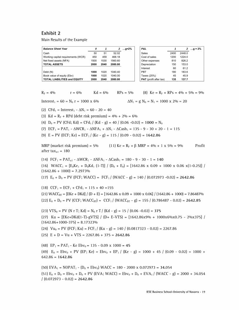
Exhibit 2 Main Results of the Example

Balance Sheet Year 0 1 2 …g=2% P&L 1 2 …g = 2%

Cash 50 51 52.02 Sales 2400 2448.0

Working capital requirements (WCR) 450 459 468.18 Cost of sales 1200 1224.0

Net fixed assets (NFA) 1500 1530 1560.60 Other expenses 810 826.2

TOTAL ASSETS 2000 2040 2080.80 Depreciation 150 153.0

Interest 60 61.2

Debt (N) 1000 1020 1040.40 PBT 180 183.6

Book value of equity (Ebv) 1000 1020 1040.00 Taxes (25%) 45 45.9

TOTAL LIABILITIES and EQUITY 2000 2040 2080.80 PAT (profit after tax) 135 137.7

RF = 4% r = 6% Kd = 6% RPs = 5% (8) Ke = RF + RPs = 4% + 5% = 9%

Interest1 = 60 = N0 r = 1000 x 6% N1 = g N0 = N1 = 1000 x 2% = 20

(2) CFd1 = Interest1 - N1 = 60 - 20 = 40

(3) Kd = RF + RPd (debt risk premium) = 4% + 2% = 6%

(4) D0 = PV (CFd; Kd) = CFd1 / (Kd - g) = 40 / (0.06 -0.02) = 1000 = N0

(7) ECF1 = PAT1 - WCR1 - NFA1 + N1 - Cash1 = 135 - 9 - 30 + 20 - 1 = 115

(9) E = PV (ECF; Ke) = ECF1 / (Ke - g) = 115 / (0.09 - 0.02) = 1642.86 MRP (market risk premium) = 5% (11) Ke = RF + MRP = 4% + 1 x 5% = 9% Profit after taxu1 = 180

(14) FCF1 = PATu1 - WCR1 - NFA1 - Cash1 = 180 - 9 - 30 - 1 = 140

(16) WACC1 = [E0Ke1 + D0Kd1 (1-T)] / (D0 + E0) = [1642.86 x 0.09 + 1000 x 0.06 x(1-0.25)] / (1642.86 + 1000) = 7.2973%

(17) E0 + D0 = PV (FCF; WACC) = FCF1 / (WACC - g) = 140 / (0.072973 -0.02) = 2642.86 (18) CCF1 = ECF1 + CFd1 = 115 + 40 =155

(21) WACCBT = [EKe + DKd] / (D + E) = [1642.86 x 0.09 + 1000 x 0.06] / (1642.86 + 1000) = 7.86487%

(22) E0 + D0 = PV (CCF; WACCBT) = CCF1 / (WACCBT - g) = 155 / (0.786487 - 0.02) = 2642.85 (23) VTS0 = PV (N r T; Kd) = N0 r T / (Kd - g) = 15 / (0.06 -0.02) = 375

(27) Ku = [EKe+DKd(1-T)-gVTS] / (D+ E-VTS) = [1642.86x9% + 1000x6%x0.75 - 2%x375] / (1642.86+1000-375) = 8.17323%

(24) Vu0 = PV (FCF; Ku) = FCF1 / (Ku - g) = 140 / (0.0817323 - 0.02) = 2267.86

(25) E + D = Vu + VTS = 2267.86 + 375 = 2642.86 (48) EP1 = PAT1 - Ke Ebv0 = 135 - 0.09 x 1000 = 45

(49) E0 = Ebv0 + PV (EP; Ke) = Ebv0 + EP1 / (Ke - g) = 1000 + 45 / (0.09 - 0.02) = 1000 + 642.86 = 1642.86 (50) EVA1 = NOPAT1 - (D0 + Ebv0) WACC = 180 - 2000 x 0.072973 = 34.054

(51) E0 + D0 = Ebv0 + D0 + PV (EVA; WACC) = Ebv0 + D0 + EVA1 / (WACC - g) = 2000 + 34.054 / (0.072973 - 0.02) = 2642.86


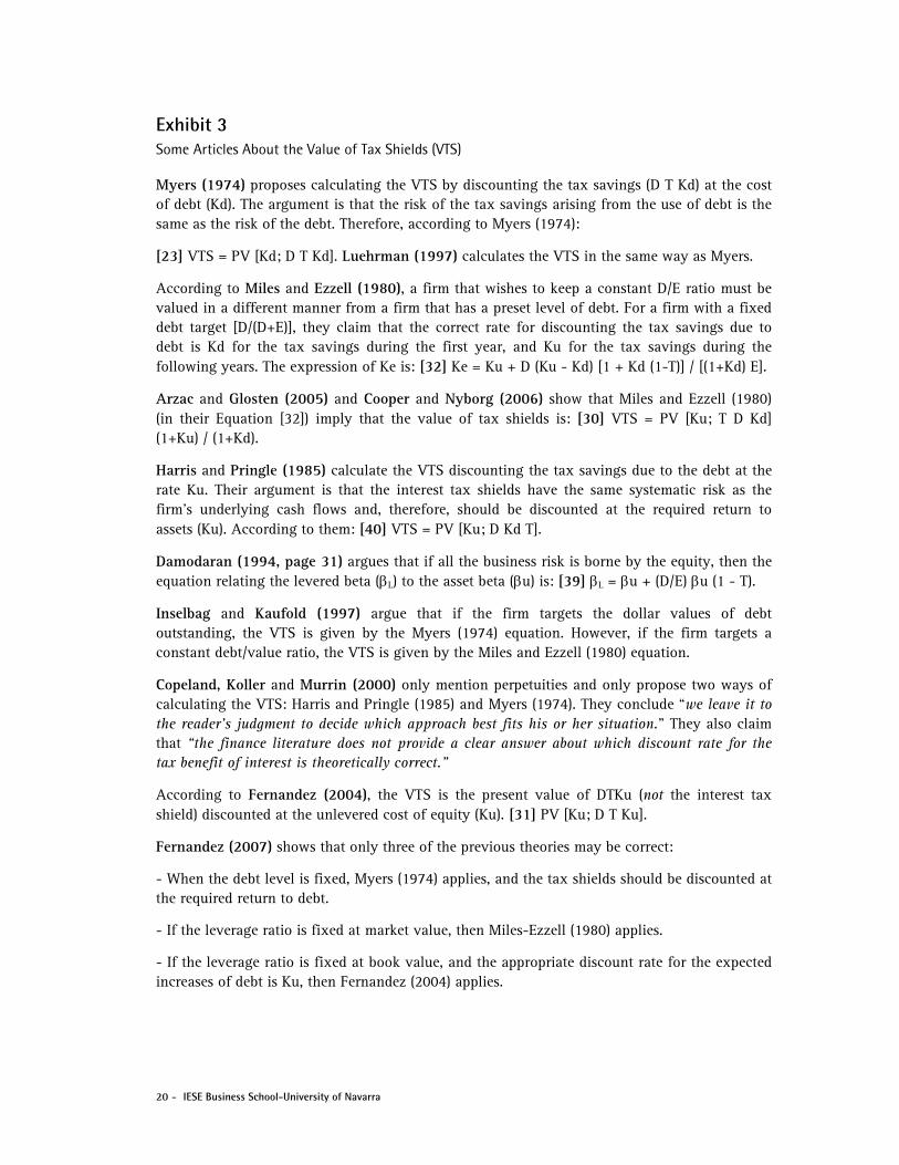
Exhibit 3 Some Articles About the Value of Tax Shields (VTS)

Myers (1974) proposes calculating the VTS by discounting the tax savings (D T Kd) at the cost of debt (Kd). The argument is that the risk of the tax savings arising from the use of debt is the same as the risk of the debt. Therefore, according to Myers (1974):

[23] VTS = PV [Kd; D T Kd]. Luehrman (1997) calculates the VTS in the same way as Myers.

According to Miles and Ezzell (1980), a firm that wishes to keep a constant D/E ratio must be valued in a different manner from a firm that has a preset level of debt. For a firm with a fixed debt target [D/(D+E)], they claim that the correct rate for discounting the tax savings due to debt is Kd for the tax savings during the first year, and Ku for the tax savings during the following years. The expression of Ke is: [32] Ke = Ku + D (Ku - Kd) [1 + Kd (1-T)] / [(1+Kd) E].

Arzac and Glosten (2005) and Cooper and Nyborg (2006) show that Miles and Ezzell (1980) (in their Equation [32]) imply that the value of tax shields is: [30] VTS = PV [Ku; T D Kd] (1+Ku) / (1+Kd).

Harris and Pringle (1985) calculate the VTS discounting the tax savings due to the debt at the rate Ku. Their argument is that the interest tax shields have the same systematic risk as the firm’s underlying cash flows and, therefore, should be discounted at the required return to assets (Ku). According to them: [40] VTS = PV [Ku; D Kd T].

Damodaran (1994, page 31) argues that if all the business risk is borne by the equity, then the equation relating the levered beta (L) to the asset beta (u) is: [39] L = u + (D/E) u (1 - T).

Inselbag and Kaufold (1997) argue that if the firm targets the dollar values of debt outstanding, the VTS is given by the Myers (1974) equation. However, if the firm targets a constant debt/value ratio, the VTS is given by the Miles and Ezzell (1980) equation.

Copeland, Koller and Murrin (2000) only mention perpetuities and only propose two ways of calculating the VTS: Harris and Pringle (1985) and Myers (1974). They conclude “we leave it to the reader’s judgment to decide which approach best fits his or her situation.” They also claim that “the finance literature does not provide a clear answer about which discount rate for the tax benefit of interest is theoretically correct.”

According to Fernandez (2004), the VTS is the present value of DTKu (not the interest tax shield) discounted at the unlevered cost of equity (Ku). [31] PV [Ku; D T Ku].

Fernandez (2007) shows that only three of the previous theories may be correct:

- When the debt level is fixed, Myers (1974) applies, and the tax shields should be discounted at the required return to debt.

- If the leverage ratio is fixed at market value, then Miles-Ezzell (1980) applies.

- If the leverage ratio is fixed at book value, and the appropriate discount rate for the expected increases of debt is Ku, then Fernandez (2004) applies.


References Arzac, E. R. and L. R. Glosten (2005), “A Reconsideration of Tax Shield Valuation,” European Financial Management 11/4, pp. 453-461.

Cooper, I. A. and K. G. Nyborg (2006), “The Value of Tax Shields IS Equal to the Present Value of Tax Shields,” Journal of Financial Economics 81, pp. 215-225.

Copeland, T. E., T. Koller and J. Murrin (2000), Valuation: Measuring and Managing the Value of Companies. Third edition. New York: Wiley.

Damodaran, A. (1994), Damodaran on Valuation, John Wiley and Sons, New York.

Fernandez, P. (2004), “The value of tax shields is NOT equal to the present value of tax shields,” Journal of Financial Economics, Vol. 73/1 (July), pp. 145-165.

Fernandez, P. (2007). “A More Realistic Valuation: APV and WACC with constant book leverage ratio,” Journal of Applied Finance, Fall/Winter, Vol.17 No. 2, pp. 13-20.

Harris, R. S. and J. J. Pringle (1985), “Risk-Adjusted Discount Rates Extensions form the Average-Risk Case,” Journal of Financial Research (Fall), pp. 237-244.

Inselbag, I. and H. Kaufold (1997), “Two DCF Approaches for Valuing Companies under Alternative Financing Strategies (and How to Choose Between Them),” Journal of Applied Corporate Finance (Spring), pp. 114-122.

Luehrman, T. A. (1997), “What’s It Worth? A General Manager’s Guide to Valuation,” and “Using APV: A Better Tool for Valuing Operations,” Harvard Business Review (May-June), pp. 132-154.

Miles, J. A. and J. R. Ezzell (1980), “The Weighted Average Cost of Capital, Perfect Capital Markets and Project Life: A Clarification,” Journal of Financial and Quantitative Analysis (September), pp. 719-730.

Miles, J. A. and J. R. Ezzell (1985), “Reequationing Tax Shield Valuation: A Note,” Journal of Finance, Vol XL, 5 (December), pp. 1485-1492.

Myers, S. C. (1974), “Interactions of Corporate Financing and Investment Decisions – Implications for Capital Budgeting,” Journal of Finance (March), pp. 1-25.

Ruback, R. S. (1995), “A Note on Capital Cash Flow Valuation,” Harvard Business School, 9-295-069.

Other downloadable articles:

Valuing Companies by Cash Flow Discounting: Ten Methods and Nine Theories http://ssrn.com/abstract=256987

Beta = 1 Does a Better Job than Calculated Betas http://ssrn.com/abstract=1406923

Betas Used in Europe: A Survey. 2009 http://ssrn.com/abstract=1419919

Equity Premium: Historical, Expected, Required and Implied http://ssrn.com/abstract=933070


Some comments from readers:

“Company valuation using discounted cash flows is based on the valuation of government bonds: it consists of applying the procedure used to value the government bonds to the debt and shares of a company.”

I would argue that because central banks are intervening in markets/government bonds like never before, using government bonds would lead to a manipulated valuation.

At the start of your paper you apply the convention that the required return on government bonds is referred to as the “risk-free rate Rf.” (“The risk-free rate (RF) is the required return to government bonds.”) As has become all too apparent during the euro crisis, government bonds cannot necessarily be considered “risk free,” and within the Euro Zone there are correspondingly marked differences between the required returns on government bonds of different countries. I would be interested to know how you cover this issue with your students, and what “risk-free rate” you advise them to use when attempting to value a Euro Zone company. Do you find yourself perhaps introducing a new “‘addition’ (formulae, concepts, theories...),” for instance, that even if a company is Spanish, the “risk-free rate” should be the rate on German government bonds? Is this then another complication, and possible source of error, that should be examined in a future update of your paper?

Very interesting, and, although I expected errors, I was amazed at how many errors in valuation calculations you found!

I have another request/reflection on your paper. My perception has always been that the DCF formula lends itself nicely to very stable and rather profitable companies. I believe it creates challenges when looking at high growth companies, especially when these are loss making for most of the DCF time frame for the analysis. The DCF method then relies heavily on the terminal value, which in turn relies on an assumed growth rate. The latter becomes a tremendous swing factor. Unfortunately, this factor is very difficult to assess for high growth companies.

Have you looked at any of the U.S. homebuilders? Homebuilders are an interesting phenomenon since they burn cash during upcycles as they acquire land for acquisition and development and generate cash during downcycles as they run off inventory. The companies also have large deferred tax assets (DTAs) that are reserved for (so not reflected on the balance sheet), although these assets require significant pre-tax income to be monetized. As a result, investors don’t typically do DCFs on these companies. Most use a multiple on book value plus some credit for DTAs or so-called normalized earnings.

I have been trying to look at alternative valuation approaches, including a land runoff model plus some equity option value as well as an excess return model.

Enterprise value to EBITDA (normalized) taking into account future enterprise value (cash flows) using a 12% discount rate (higher if the company’s debt yields higher). Add back hidden assets such as tax shields for NOLs.

I’m a practitioner in the sense that I’ve practiced private equity for 23 years now, and that I chair the French PE association (AFIC). My firm (Argos Soditic) also publishes the only index of valuation for unlisted companies in the Euro Zone (cf. our website).


In a nutshell:

DCF is monstrous, in the genetic sense. It mixes in the same calculation historic data (betas, risk premium…), spot data (government bond rates) and forward data. As you rightly point out, because it’s very complex it gives a false sense of “hard scientific” results. One can claim it’s the basis of most of the recent financial disasters (subprimes, .com bubble, and farther away Eurotunnel, etc.).

The main issue with DCF and many valuation models is that they rely on forecasting. You know what Galbraith said of economic forecasting and astrology, and he was definitely right. Let me share a secret with you: since I started PE, I’ve never ever managed to exit an investment with an IRR within an 8% range (meaning -8% / +8%) of the initial IRR target. Never. (For the avoidance of doubt, my firm is said by its investors to be top decile; we’re one of the very few to have raised a fund recently and it’s been massively oversubscribed, so supposedly we have some investor skills). Why that failure, despite all the efforts, money and external advice in forecasting? My (interim) conclusion is that forecasting and forecast-based valuation are close to being meaningless for companies, while they remain valid for assets with predictable cash flows (say, a photovoltaic farm). When investing in a business you have to accept that uncertainty is the rule, and worse: you can be certain that something unpredictable will happen; therefore, success relies on the ability to ride into uncertainty, hence you focus much more on management capabilities, governance, etc.

So how do we value companies? Well, at least half of the thinking relies on a basic, stupid EV/(EBITDA-Capex) ratio. And my analysts are forbidden to run DCFs. Waste of time… and loss of critical spirit on forecasts.

Not sure this helps in your work, but the success factors in this game appear to be in soft factors, and first of all people, more than any model.

The article could be better if the following were to be considered:

– How and where to get those inputs for estimation.

– Rather than say B/S and P/L grow at 2%, maybe you could say the reinvestment growth rate is 2%. More explanations on computation of reinvestment growth rate, how it related to the company’s capital structure.

– Net fixed assets may be replaced with net non-current assets to be in line with the terminology used by International Financial Reporting Standards.

– Tax rate may need to be further clarified between statutory tax rate and effective tax rate, where the later is used in estimation.

– Brief on market value added and DDM model.

– How to reconcile the values produced by different formula used and the weights to be given to each value.

– Show by example the material impact on value if wrong input is used such as discount rate, growth rate...

– Current sovereign debt crisis may impact the concept of “risk-free rate of return;” government may default, especially now in Europe!


I have one remark when it comes to NPV calculations:

People do these by estimating future cash flow – and then discount these back with WACC. And then subtract the net debt from the resulting EV to find the Eq-value. I do, however, believe this overestimates the NPV (and by the way – I always find the NPV to be larger than multiple-based methods [for several reasons – but one important one is due to the following fact]).

I do not agree on using a WACC on the cash flow – I think a WACC should be used on the income and corresponding “uncertain” costs (i.e., variable), and then discount all other (fixed) costs with only cost of capital (not risk-adjusted), for example, a secure government bond rate. This is because these (cost) elements of the WACC now have uncertainty, they will appear anyway, and should hence not be reduced by this big WACC.

VALUING COMPANIES BY CASH FLOW DISCOUNTING: …

Documents

Transcript of VALUING COMPANIES BY CASH FLOW DISCOUNTING: …