VALUING BOND FUTURES AND THE QUALITY OPTION

by

Peter Carr

Morgan Stanley

Equity Derivatives Research

1585 Broadway, 6th Fl.

New York, New York 10036

(212) 761-7340

and

Ren-Raw Chen*

Faculty of Management

SOB/NB, Department of Finance

Rutgers University

Janice Levin Bldg., Livingston Campus

New Brunswick, NJ 08903

(908) 445-4236

February, 1997

* This paper is a revision of the paper under the same title by Peter Carr. We would li ke to thank MichaelBrennan, Eduardo Schwartz, Sheridan Titman, David Butz, Bryan Elli ckson, Warren Bailey, BrunoGerard, David Hirshleifer, Craig Holden, Farshid Jamshidian, Walter Torous, and Louis Scott forcomments and Gikas Hardouvelis for the T-Bill data. Carr would li ke to thank an Allstate DissertationFellowship from UCLA and Chen would li ke to thank the CBOT Educational Research Foundation forfinancial support.

VALUING BOND FUTURES AND THE QUALITY OPTION

ABSTRACT

This paper develops a model for determining Treasury bond futures prices when the short

position has a quality option. The model is developed in a general equili brium economy

where futures prices are driven by one or two factors. The main advantage of a factor

based model over the exchange option based model is the abili ty to permit a realistic

number of bonds in the deliverable set. The two factor quality option model is tested

against two popular models which ignore the quality option, namely the CIR model (1981)

and the cost of carry model using the cheapest to deliver bond.

1

1 INTRODUCTION

The Chicago Board of Trade's US Treasury Bond futures contract is one of the most

actively traded securities in history. Given its volume, it is not surprising that there has

been considerable interest in developing accurate pricing models for these contracts.

Historically, the futures price has been below that predicted by the traditional cost-

of-carry model.1 This deficiency has been attributed to several delivery options which the

short retains. Kane and Marcus (1986) categorize these options as either timing options

or quality options. Timing options have value because the short may deliver on any

business day in the delivery month. Additional value arises because trading in the cash

market continues after the futures price has settled.2

The quality option gives the short position the opportunity to deliver any US

Treasury bond that has at least fifteen years to maturity or first call. Currently, more than

thirty bonds, widely varying in coupon, callabili ty and maturity, meet these criteria. The

empirical evidence suggests that it is extremely difficult to predict which bond will be

optimally delivered by the short. A system employing conversion factors for the various

bonds has been developed by the Chicago Board of Trade (CBOT) in an effort to mitigate

the scope of the short's option. However, the profitabili ty of each position still depends

heavily on which bond is delivered, after accounting for the effect of conversion factors.

For this reason, the long position in the futures contract is said to face conversion factor

risk.

Models for the quality option in Treasury bond futures can be divided into those

which assume a stochastic process directly on bond prices and those which model interest

rates instead. The former class of models includes Cheng (1985), Chowdry (1986),

Hemler (1990) and Boyle (1989). The latter class of models includes Cox, Ingersoll, and

Ross (1981), Ritchken and Sankarasubramanian (1992), Cherubini and Esposito (1996),

and Bick (1996). We also develop and test a model of the quality option based upon the

term structure of interest rates.

We develop tractable procedures in a general equili brium economy where futures

prices are driven by one or two factors, rather than by the prices of over thirty different

bonds. In a series of papers, Vasicek (1977), Richard (1978), Brennan and Schwartz

1 The traditional cost-of-carry model relates the futures price to the spot price of the underlying asset,which in this case is the bond which is currently cheapest to deliver.2 For the first 15 or 16 days of each delivery month, there is a 6 hour period during which the cash marketremains open after the futures price has been settled. Futures trading ceases entirely for the last 7 tradingdays. These options have been termed the wild card option and the end-of-the-month option respectively.

2

(1979), Courtadon (1982) and Cox, Ingersoll and Ross (1985, hereafter CIR) have

developed a methodology for pricing interest rate dependent claims. The methodology

has been applied to determining bond spot and futures prices. This paper extends this

methodology towards determining bond futures prices when the short position has a

quality option.

In the one factor case, a closed form solution is developed which requires

evaluating only univariate distribution functions. A more general two factor model can be

extended from the one factor model in a number of ways. CIR (1985) develop several

two and three factor models of the term structure. Using the same methodology as CIR,

Longstaff and Schwartz (1992) derive a two factor term structure model in which the

short rate and the volatili ty move randomly. Chen and Scott (1992) also follow the CIR

framework and decompose the spot rate into two factors. Jamshidian (1993) and Duffie

and Kan (1992) extend the Chen and Scott model to an arbitrary number of factors.

Aside from increased tractabili ty, a term structure approach has several other

advantages over models which specify bond price diffusions directly. One advantage is the

paucity of inputs required to calculate the futures price, when there are a realistic number

of bonds in the deliverable set. For our model, one needs only the values of at most two

interest rates rather than the prices of over thirty different bonds. In contrast, when over

thirty bonds are deliverable, over 465 bond return variances and covariances must be

estimated3 to implement models which specify bond price diffusions. Furthermore, those

models generally do not preclude negative spot or forward rates of interest.4 Moreover,

the models employing bond price diffusions must assume that the coupon is a constant

fraction of the bond price in order to obtain analytical solutions. Since bond coupons are

constant, there is an internal inconsistency in these models unless the coupon rate is

assumed to be zero. In contrast, term structure approaches allow for constant coupons.

Finally, generalizing the analysis to allow for the callabili ty feature of several of the

underlying bonds is much more easily handled in a term structure framework. Including

the call feature is particularly important because it increases the likelihood that the bond is

optimally delivered.

The plan of this work is as follows. In Section II , we develop a model where the

short rate of interest is taken as the single state variable. Analytic valuation formulae are

obtained for the futures price with the quality option. Since the CBOT quality option is

3 Imposing a single factor asset pricing model such as the CAPM reduces the number of parameters to beestimated.4 An important exception is Flesaker and Hughsten (1996). It would be interesting to apply theirapproach to quality options.

3

over long term bonds, the state space is augmented in Section III with a second factor that

takes into account the effect of the long rate of interest. Section IV provides an empirical

study of the two factor model. Section V concludes the paper.

2 ONE FACTOR MODEL

2.1 Assumptions and Notation

The following assumptions describe the structure of the model:

A1) Perfect Spot and Futures Markets

There are no transactions costs, margin requirements, limit moves, indivisibilities,

differential taxes or short selling restrictions. Trading and marking-to-market occur

continuously in time.

The import of this assumption is to rule out frictions of any sort and to cast the analysis in

continuous time and space. In reality, marking-to-market occurs daily5 and prices move in

thirty seconds of a point subject to a three point daily price limit.

A2) Delivery Process

Delivery occurs at the contract expiration date. The short receives the futures price

times the relevant conversion factor.

This assumption simplifies the analysis by excluding the short’s timing option from

consideration. The timing option will have smaller relative value when considering long

maturity futures contracts.

A3) Deliverable Set

The coupon rate and maturity of all bonds in the deliverable set is known on the

valuation date.

This assumption eliminates uncertainty as to the terms of any bonds issued between the

valuation date and expiration. Since Treasury bonds are issued quarterly, this assumption

is less valid for longer maturity contracts. If an eligible bond is callable, the assumption

also eliminates uncertainty as to the call date.

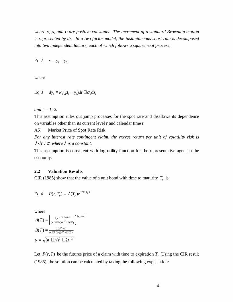
A4) Mean Reverting Square Root Process

In the one factor model, the following dynamics is assumed for the instantaneous rate:

Eq 1 dr r dt rdz= − +κ µ σ( )

5 Flesaker (1988) and Chen (1991) have shown that the effect of dail y marking to market on the futuresprice differs very little from that of continuous marking to market.

4

where κ, µ, and σ are positive constants. The increment of a standard Brownian motion

is represented by dz. In a two factor model, the instantaneous short rate is decomposed

into two independent factors, each of which follows a square root process:

Eq 2 r y y= +1 2

where

Eq 3 dy y dt dzi i i i i i= − +κ µ σ( )

and i = 1, 2.

This assumption rules out jump processes for the spot rate and disallows its dependence

on variables other than its current level r and calendar time t.

A5) Market Price of Spot Rate Risk

For any interest rate contingent claim, the excess return per unit of volatility risk is

λ σr / where λ is a constant.

This assumption is consistent with log utili ty function for the representative agent in the

economy.

2.2 Valuation ResultsCIR (1985) show that the value of a unit bond with time to maturity Tp is:

Eq 4 P r T A T ep p

rB Tp( , ) ( ) ( )= −

where

[ ]A T

B T

e

e

e

e

T

T

T

T

( )

( )

( )

( ) /

( )(

/

(

( )(

=

=

= + +

+ +

+ + − +

−+ + − +

2

1) 2

2

2 1)

1) 2

2 2

22

2

γκ λ γ γ

κµ σ

κ λ γ γ

κ λ γ

γ

γ

γ

γ κ λ σ

Let F r T( , ) be the futures price of a claim with time to expiration T. Using the CIR result

(1985), the solution can be calculated by taking the following expectation:

5

Eq 5 F r T T E P r Tp f p p( , ; )�

[ (~, )]=

In the above equation, ~r is the terminal spot rate and �

[ ]E ⋅ denotes expectations under the

following risk-neutralized process:

Eq 6 dr r r dt rdz= − − +[ ( ) ]�

κ µ λ σ

It can be shown that the expectation of Eq 5 under Eq 6 leads to CIR’s formula for the

futures price of a pure discount bond (1981):

Eq 7 F r T T C T ep f p f

rD Tf( , , ) ( ) ( )= −

where

[ ]C T A T

D T B T

f B T p

fe

B T p

e

p

Tf

p

Tf

( ) ( )

( ) ( )

( )

/

( )

( )

(1 )

( )

( )

=

=

=

+

+

+

−

− +

− +

ηη

κµ σ

ηη

κ λσ

κ λ

κ λη

2

2

2

2

Both the spot and futures prices of the pure discount bond are decreasing, convex

functions of the spot rate r. While the spot price of the bond is declining in its time to

maturity Tp , the futures price may be increasing or decreasing in the time to expiration

Tf , ceteris paribus. Since the futures price is nothing more than an expectation under a

certain process, there is no reason why changing the expiration date should unambiguously

affect the futures price.

By CIR (1981), the futures price of a coupon bond, F r Tb f( , ) , can be specified as

follows:

Eq 8

F r T E B r T

C E P r T

C F r T T

b f b

j

b

j j

j

b

j p f j

( , )�

[ (~, )]

�

[ (~, )]

(~, ; )]

=

=

=

=

=

∑

∑1

1

6

where

Eq 9 B r T C P r Tb jb

j j(~, ) (~, )= =Σ 1

and C j is the coupon for j b= −1 1, ,� and the coupon plus face value for j b= .

Next, we calculate the futures price, F r Tb f( ) ( , )2 , when the short can deliver either

of two Treasury bonds. Of course, the short selects the bond which maximizes his profit,

after accounting for the conversion factors qi ,6 which leads to the following terminal

condition:

Eq 10 F rB r T

q

B r T

qbb b( ) ( , ) min

(~, ),

(~, )2 1

1

2

2

0 =

The terminal futures price is just the smaller of the two “adjusted” bond prices, where the

adjustment occurs by dividing each bond’s price by its conversion factor. Depending on

the coupons and maturities of the two bonds, one bond may be cheaper to deliver for all

terminal interest rates, or one bond may be preferred for certain rates, while the other

bond is preferred for different rates. In the former case, Eq 8 applies for the cheaper to

deliver bond. In the latter case, the adjusted price of the cheaper bond must be determined

for each level of the short rate at expiration. Suppose for simplicity that bond 1 is cheaper

for interest rates below some critical level r * while bond 2 is cheaper for higher rates.

Then:

Eq 11

F r T EB r T

q

B r T

q

B r T

q

B r T

qr dr

B r T

qr dr

B r T

qr dr

b fb b

b b

rb

r

b

( ) ( , )�

min(~, )

,(~, )

min(~, )

,(~, )

(~) ~

(~, )(~) ~ (~, )

(~) ~*

*

2 1

1

2

2

0

1

1

2

2

0

1

1

2

2

=î

=î

= +

∞

∞

∫

∫ ∫

φ

φ φ

6 The conversion factor is the fraction of par value for which the bond would sell , if it were priced to yield8%.

7

where φ(~)r is the probabili ty density function of the terminal interest rate under the drift-

adjusted mean-reverting square root process Eq 6. The Appendix presents this density

function en route to proving the following result which is used to evaluate Eq 11:

Eq 120

1

2 2r

b

j

bj

p f j j

B r T

qr dr

C

qF r T T B T r v

* (~, )(~) ~ ( , ; ) [ ( ( )) ; , ]*∫ ∑= +

=

φ χ η Λ

where χ 2[ ; , ]x v Λ is the non-central chi-square distribution function evaluated at x with

v = 4 2κµ σ/ degrees of freedom and noncentrality parameter Λ = − ++

2 2η κ λη

exp( ( ) )

( )

T

B Tf

jr .

Applying this result to Eq 11 implies that the current futures price is:

Eq 13 F r TC

qF r T T r

C

qF r T T rb f

j

bj

p f jj

bj

p f j( ) * *( , ) ( , ; ) ( ) ( , ; ) ( )2

1

11

1

2

1

22

2

2= += =∑ ∑χ χ

where χ χ η2 2 2( ) [ ( ( )) ; ; ]* *r B T r vj= + Λ .

2.3 Multiple Crossover Points

The pricing equation Eq 13 is predicated on there being at most one crossover point for

the two underlying bond prices at expiration. Theoretically, there is no reason why the

prices of the two bonds cannot cross themselves more than once. Furthermore, in any

delivery month, there are 20 to 30 bonds deliverable against the CBOT Treasury bond

futures contract. Fortunately, the biggest problem in extending our results to an arbitrary

number of crossover points and deliverable bonds in mainly notational. The terminal

condition when n bonds are deliverable is:

Eq 14 F rB r T

q

B r T

qbn b b( ) (~, ) min

(~, ), ,

(~, )0 1

1

2

2

=

�

Employing the same technique as used to derived Eq 12, the current futures price

generalizes to :

Eq 15 F r TC

qF r T T wb

nf

j

bij

ip f j ij

i

n( ) ( , ) ( , ; )=

==∑∑

11

8

where w I r rij km

ik j k j k= − >= −Σ 12 2

1 0[ ( ) ( )]* *χ χ , i n= 1, � , j bi= 1, � , are weights summing

to unity across bonds. i.e. Σ in

ijw= =1 1 for all j, and where r k mk* , , , ,= 01 � are crossover

points arranged in increasing order as 0 0 1 1= < < < < = ∞−r r r rm m* * * *

� . Iik is an indicator

variable equal to one if bond i is cheapest in the interval and 0 otherwise, i =1,2.

Eq 15 is easier to use than its formal form might suggest. Figure 1 ill ustrates that

if there are only three bonds which are cheapest to deliver in their respective subinterval,

then Eq 15 will consist of only three terms, each of which is the futures price of the bond

integrated against the probability kernel over the relevant spot rate range.

Figure 1: Three Adjusted Bond Prices Crossing Twice

The CBOT futures price is a weighted average of the futures prices of the

component cash flows of each deliverable bond. The weight applied reflects7 the

probabili ty (risk neutral) that the cash flow belongs to the cheapest deliverable bond at

expiration. The futures price is a decreasing convex function of the current short rate r. It

may be decreasing or increasing in the time to expiration, holding the underlying bond

maturities constant.

Eq 15 can be used to develop the cost-of-carry relationship between the futures

price and the underlying bond prices. Recall that Bi is the bond price of the i-th bond.

Then:

Eq 16 F r T x Bbn

fi

n

i i( ) ( , ) =

=∑

1

where xi jb C F r T T w

q Bij p f j ij

i i= =Σ 1

( , , ).

Unlike the traditional cost-of-carry model, our model relates the futures price to

several underlying bond prices. Eq 16 also indicates that the long position can eliminate

conversion factor risk by always shorting xi units of the i-th bond. At maturity, the long

will only be shorting the cheapest deliverable bond. He can then use the bond received

from his long position to cover this short.

7 Note that the weight does not equal this probabilit y but reflects it in that wij is increasing in theprobability and equals 0 and one when the probability does.

9

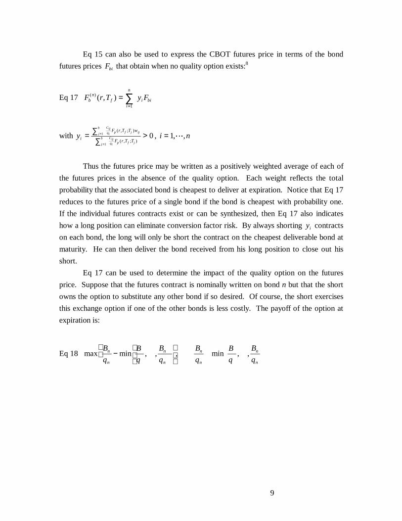
Eq 15 can also be used to express the CBOT futures price in terms of the bond

futures prices Fbi that obtain when no quality option exists:8

Eq 17 F r T y Fbn

fi

n

i bi( ) ( , ) =

=∑

1

with yi

F r T T w

F r T T

j

b Cijqi p f j ij

j

b Cijqi p f j

= ∑∑

>=

=

1

1

0( , ; )

( , ; ), i n= 1, ,�

Thus the futures price may be written as a positively weighted average of each of

the futures prices in the absence of the quality option. Each weight reflects the total

probabili ty that the associated bond is cheapest to deliver at expiration. Notice that Eq 17

reduces to the futures price of a single bond if the bond is cheapest with probabili ty one.

If the individual futures contracts exist or can be synthesized, then Eq 17 also indicates

how a long position can eliminate conversion factor risk. By always shorting yi contracts

on each bond, the long will only be short the contract on the cheapest deliverable bond at

maturity. He can then deliver the bond received from his long position to close out his

short.

Eq 17 can be used to determine the impact of the quality option on the futures

price. Suppose that the futures contract is nominally written on bond n but that the short

owns the option to substitute any other bond if so desired. Of course, the short exercises

this exchange option if one of the other bonds is less costly. The payoff of the option at

expiration is:

Eq 18 max min , , , min , ,B

q

B

q

B

q

B

q

B

q

B

qn

n

n

n

n

n

n

n

−

î

= −

−

−

1

1

1

1

1

1

0� �

Consequently, the current futures price of this option is given by:

Eq 19�

min , , ( )( )EB

q

B

q

B

qF F F y F yn

n

n

nn b

nn n

i

n

i i−î

= − = − −

=

−

∑1

1 1

1

1�

8 For simplicity, we assume that the conversion factor system still exists in that the invoice price resultingfrom delivery of bond i is qiFbi

10

Eq 19 shows that the bond futures price is affected by the futures price of the

quality option rather than its spot price. As in most option pricing modes, Eq 19 shows

that the (futures) price of the option is a probabili ty-weighted difference in the (futures)

prices of the optioned asset and the exercise asset. The weight on the futures price of the

nominal bond is related to the probabili ty that this bond is not cheapest to deliver. This

weight measures the likelihood that the quality option finishes in the money. The weights

on the futures prices of the other bonds reflect their respective probabilities of delivery.

3 TWO FACTOR MODEL

A disadvantage of single factor models is that bond returns of different maturities are

perfectly correlated locally. Another disadvantage that arises when the single factor is the

spot rate is that insufficient variance is generated for long term bond prices. In fact, as the

time to maturity tends to infinity, the bond yield approaches a constant. As the CBOT

quality option is defined over long term bonds and its value is sensitive to the underlying

bond variances, a second factor is needed in order to induce the variabili ty observed in

long interest rates.

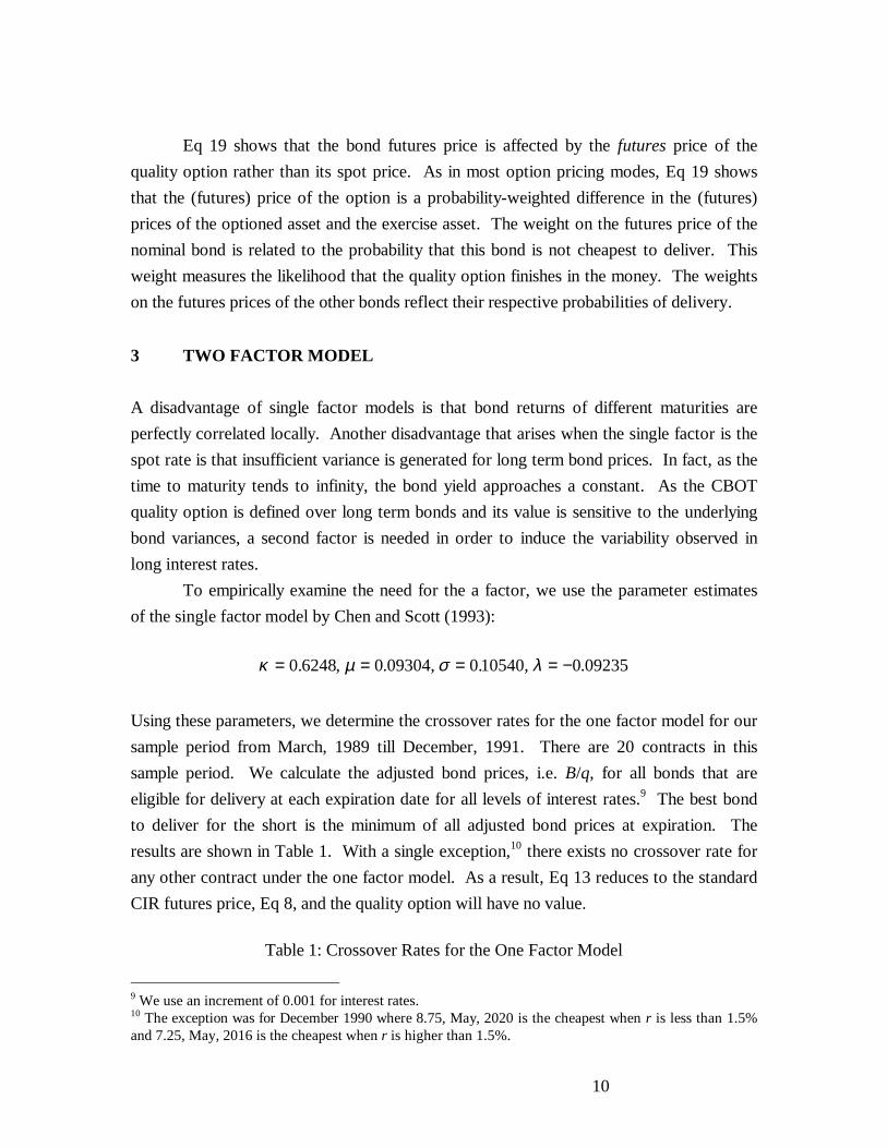
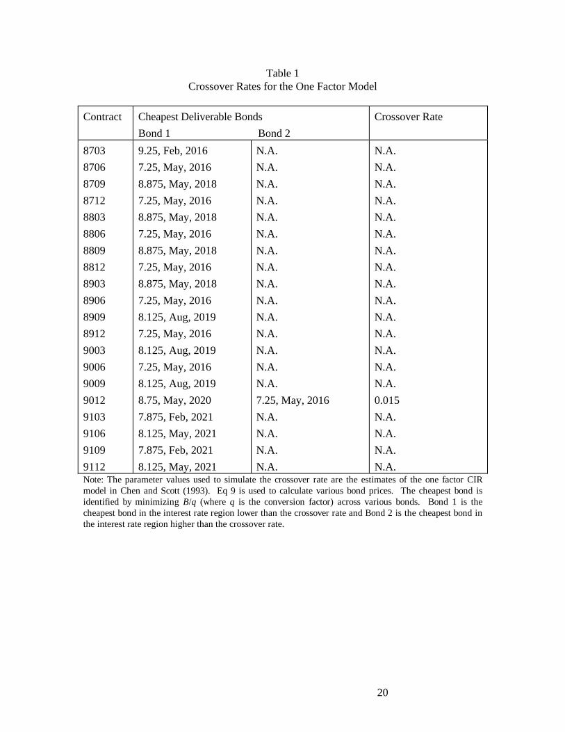
To empirically examine the need for the a factor, we use the parameter estimates

of the single factor model by Chen and Scott (1993):

κ µ σ λ= = = = −0 6248 0 09304 010540 0 09235. , . , . , .

Using these parameters, we determine the crossover rates for the one factor model for our

sample period from March, 1989 till December, 1991. There are 20 contracts in this

sample period. We calculate the adjusted bond prices, i.e. B/q, for all bonds that are

eligible for delivery at each expiration date for all levels of interest rates.9 The best bond

to deliver for the short is the minimum of all adjusted bond prices at expiration. The

results are shown in Table 1. With a single exception,10 there exists no crossover rate for

any other contract under the one factor model. As a result, Eq 13 reduces to the standard

CIR futures price, Eq 8, and the quality option will have no value.

Table 1: Crossover Rates for the One Factor Model

9 We use an increment of 0.001 for interest rates.10 The exception was for December 1990 where 8.75, May, 2020 is the cheapest when r is less than 1.5%and 7.25, May, 2016 is the cheapest when r is higher than 1.5%.

11

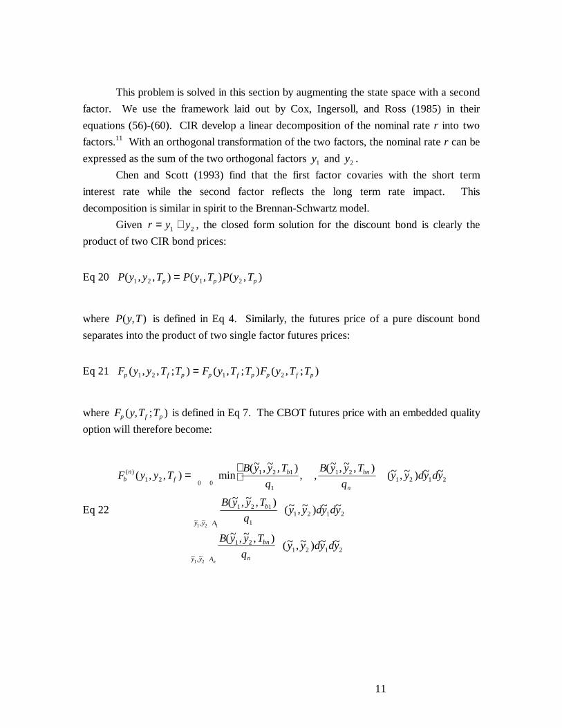
This problem is solved in this section by augmenting the state space with a second

factor. We use the framework laid out by Cox, Ingersoll, and Ross (1985) in their

equations (56)-(60). CIR develop a linear decomposition of the nominal rate r into two

factors.11 With an orthogonal transformation of the two factors, the nominal rate r can be

expressed as the sum of the two orthogonal factors y1 and y2 .

Chen and Scott (1993) find that the first factor covaries with the short term

interest rate while the second factor reflects the long term rate impact. This

decomposition is similar in spirit to the Brennan-Schwartz model.

Given r y y= +1 2 , the closed form solution for the discount bond is clearly the

product of two CIR bond prices:

Eq 20 P y y T P y T P y Tp p p( , , ) ( , ) ( , )1 2 1 2=

where P y T( , ) is defined in Eq 4. Similarly, the futures price of a pure discount bond

separates into the product of two single factor futures prices:

Eq 21 F y y T T F y T T F y T Tp f p p f p p f p( , , ; ) ( , ; ) ( , ; )1 2 1 2=

where F y T Tp f p( , ; ) is defined in Eq 7. The CBOT futures price with an embedded quality

option will therefore become:

Eq 22

F y y TB y y T

q

B y y T

qy y dy dy

B y y T

qy y dy dy

B y y T

qy y dy dy

bn

fb bn

n

y y A

b

y y A

bn

nn

( )

~ ,~

~ ,~

( , , ) min(~ ,~ , )

, ,(~ ,~ , )

(~ ,~ ) ~ ~

(~ ,~ , )(~ ,~ ) ~ ~

(~ ,~ , )(~ ,~ ) ~ ~

1 2 0

1 2 1

1

1 2

0 1 2 1 2

1 2 1

11 2 1 2

1 21 2 1 2

1 2 1

1 2

=î

= + ⋅⋅ ⋅

∞∞

∈

∈

∫∫

∫∫

∫∫

� φ

φ

φ

where ~yi is the terminal factor level, i = 1,2, Ak indicates the region of the state space

where bond k is cheapest to deliver, and where A A An1 22∪ ∪ ∪ = ℜ +

� is the whole space.

11 See the original paper pp. 404-405 for details.

12

Using the same technique as in the Appendix, we can write the integrals in terms of

bivariate non-central chi-squared distributions:

Eq 23

F y y TC

qF y y T T x x dx dx

C

qF y y T T x x dx dx

bn

fj

bij

p f j

x x A

j

bnij

np f j

x x An

( )

~ ,~

~ ,~

( , , ) ( , , ; ) (~ ) (~ ) ~ ~

( , , ; ) (~ ) (~ ) ~ ~

1 21

1

11 2 1 2 1 2

11 2 1 2 1 2

1 2 1

1 2

= +⋅⋅⋅= ∈

= ∈

∑ ∫∫

∑ ∫∫

φ φ

φ φ

where ~ ( ( ))~x B T yi j i= +2 η , for i = 1,2 and φ(~ )x i is a non-central chi-squared density

function. A closed form solution to this integral is diff icult to obtain because the domain

of each integral is a complicated region. Although the double integrals can be computed

numerically, we actually implemented a lattice model which Longstaff and Schwartz

(1992) advocate as equally efficient.

4 EMPIRICAL STUDY

In this section, we empirically examine our model, Eq 23, by comparing it against the CIR

futures pricing model which does not incorporate the quality option and the popular cost

of carry model (COC) assumes that the cheapest to deliver (CTD) bond at maturity is the

current CTD bond.

4.1 Methodology

The model used in the empirical test is the two factor model of Eq 23. The model is a sum

of two dimensional integrations. These integrals require CTD regions to be identified

first. To identify the relevant regions, we need parameter values. There have been drastic

developments in estimation techniques in recent years.12 In this paper, we use the two

factor model estimated by Chen and Scott (1993) with a weekly data set from 1980 to

1988. Their two factor model fits the yield curve reasonably well (for both in sample,

1980-88, and out of sample, 1989-91, periods). Three month, six month, five year, and

the longest maturity Treasury issues are used to estimate the parameters for the two factor

model as follows:

12 For maximum likelihood estimation, see Chen and Scott (1993) and Pearson and Sun (1993); forGenerali zed method of moments, see Gibbons and Ramaswamy (1993) and Heston (1989); for the statespace model with Kalman filtering, see Lund (1994), Chen and Scott (1995) and Duan and Simonato(1995).

13

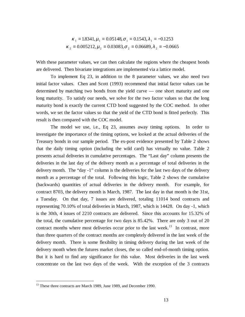
κ µ σ λκ µ σ λ

1 1 1 1

2 2 2 2

18341 0 05148 01543 01253

0 005212 0 03083 0 06689 0 0665

= = = = −= = = = −

. , . , . , .

. , . , . , .

With these parameter values, we can then calculate the regions where the cheapest bonds

are delivered. Then bivariate integrations are implemented via a lattice model.

To implement Eq 23, in addition to the 8 parameter values, we also need two

initial factor values. Chen and Scott (1993) recommend that initial factor values can be

determined by matching two bonds from the yield curve — one short maturity and one

long maturity. To satisfy our needs, we solve for the two factor values so that the long

maturity bond is exactly the current CTD bond suggested by the COC method. In other

words, we set the factor values so that the yield of the CTD bond is fitted perfectly. This

result is then compared with the COC model.

The model we use, i.e., Eq 23, assumes away timing options. In order to

investigate the importance of the timing options, we looked at the actual deliveries of the

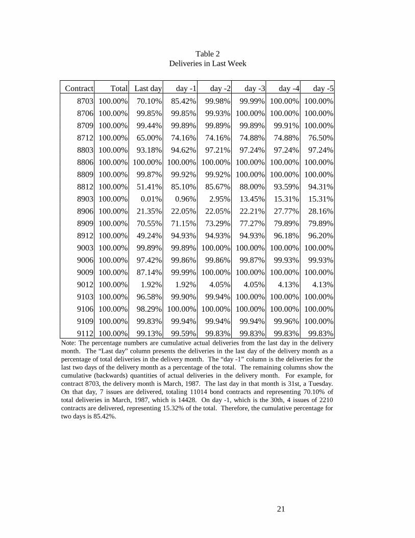
Treasury bonds in our sample period. The ex-post evidence presented by Table 2 shows

that the daily timing option (including the wild card) has virtually no value. Table 2

presents actual deliveries in cumulative percentages. The “Last day” column presents the

deliveries in the last day of the delivery month as a percentage of total deliveries in the

delivery month. The “day -1” column is the deliveries for the last two days of the delivery

month as a percentage of the total. Following this logic, Table 2 shows the cumulative

(backwards) quantities of actual deliveries in the delivery month. For example, for

contract 8703, the delivery month is March, 1987. The last day in that month is the 31st,

a Tuesday. On that day, 7 issues are delivered, totaling 11014 bond contracts and

representing 70.10% of total deliveries in March, 1987, which is 14428. On day -1, which

is the 30th, 4 issues of 2210 contracts are delivered. Since this accounts for 15.32% of

the total, the cumulative percentage for two days is 85.42%. There are only 3 out of 20

contract months where most deliveries occur prior to the last week.13 In contrast, more

than three quarters of the contract months are completely delivered in the last week of the

delivery month. There is some flexibili ty in timing delivery during the last week of the

delivery month when the futures market closes, the so called end-of-month timing option.

But it is hard to find any significance for this value. Most deliveries in the last week

concentrate on the last two days of the week. With the exception of the 3 contracts

13 These three contracts are March 1989, June 1989, and December 1990.

14

previously mentioned, all the contracts had more than 70% of the deliveries occurring

during the last two days.14

Table 2: Deliveries in Last Week

4.2 Data

In this empirical study, we use daily settlement futures prices from January, 1987 through

December, 1991. We select this sample period because we would like to conduct both in-

sample and out-of-sample tests. The Chen-Scott parameter values are estimated for the

period 1980-1988. Therefore our sample period covers the in-sample period, 87-88, and

the out-of-sample period, 89-91. The data set was acquired directly from the CBOT. We

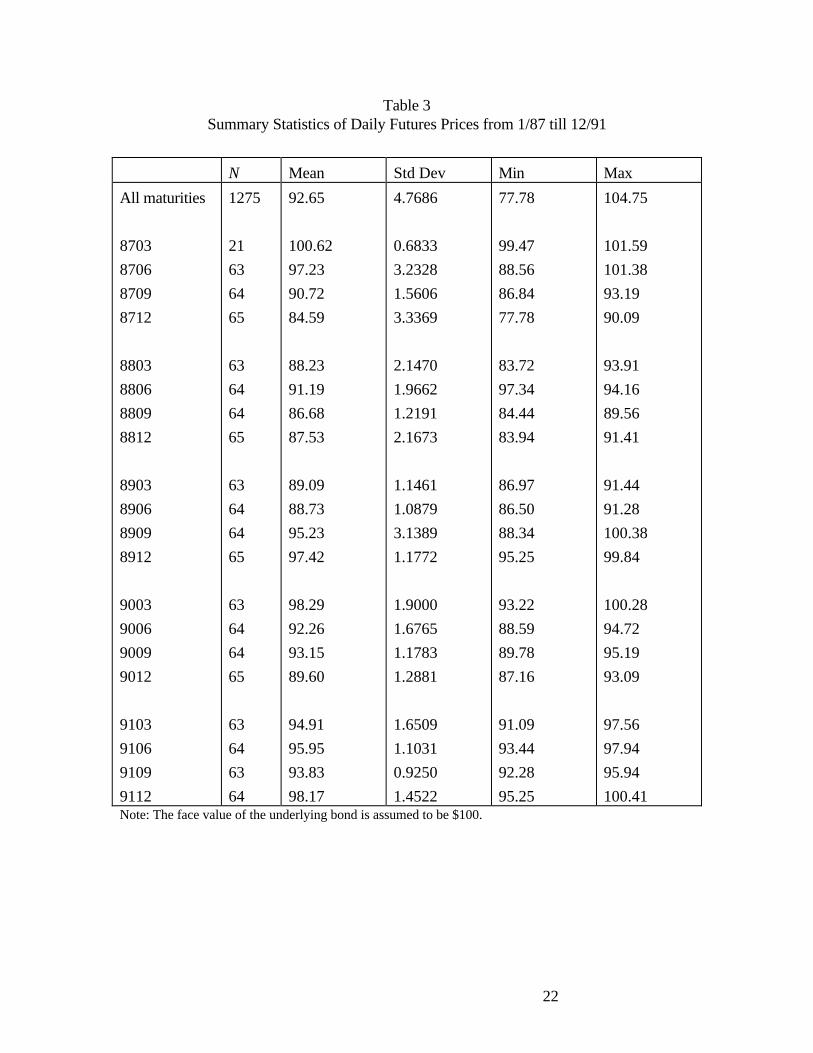
select prices of contracts that have maturities between 6 weeks and 4.5 months because of

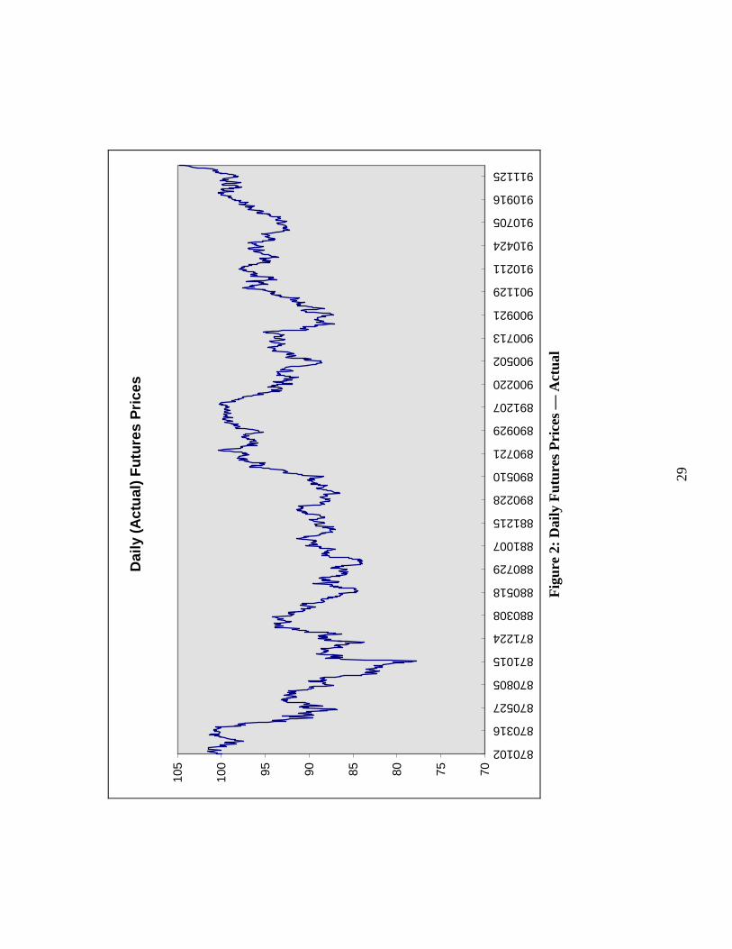
their liquidity and interest to traders.15 Figure 2 presents a plot of futures prices. Since

prices are taken from contracts that have 6 weeks to 4 and half months to maturity, there

is little overlapping of any two consecutive contracts. In other words, for every trading

day, we have only price. Table 3 breaks the time series down by the maturity of the

contract. For a given contract month, the fluctuation is smaller and we can discern a

definite pattern in the prices. Futures prices start out high, plunge in the middle of the

sample period, and then climb back by the end of the sample period. It is also seen that

prices are more volatile in 1987 and 1988 and stabilize after 1989.

Table 3: Summary Statistics of Daily Futures Prices

Figure 2: Daily Futures Prices

4.3 Results – Daily TestingTo calculate theoretical futures prices using Eq 23, we need the two factor values, y1 and

y2 daily. To calculate daily factor values for our study, we would need all deliverable

bond prices daily, which is diff icult to handle. Fortunately, Chen and Scott (1993) have

shown that the sum of the two factors which should yield the theoretical instantaneous

rate approximates extremely well the 3 month T Bill rate. As a result, we shall use daily 3

month Treasury bill rates to back out the second factor value with weekly updating the

first factor. This approximation should have little effect on our model futures prices

14 The data of actual deli veries are obtained from CBOT Financial Updates and CBOT Financial FuturesProfessional.15 This selection of maturities was based upon a conversation with CBOT.

15

because the first factor contributes very little (less than 1%, see Chen and Scott (1993)) to

the long term bond variabili ty. The 1275 daily factor values for the second factor are

calculated from January 1987 through December 1991.16

Before using Eq 23 to calculate theoretical prices, we need to identify all possible

deliverable bonds at maturity. This is accomplished by simulating all bond prices at

delivery dates. We select all deliverable bonds for every delivery month in the sample

period (8703 through 9112), calculate their theoretical prices using Eq 9 and Eq 20, and

use their conversion factors to identify the cheapest bonds for various interest rate regions.

The results are reported in Table 4.

Table 4: Deliverable Bonds in the Two Factor Model

Table 4 presents a sharp contrast to Table 1. All contracts now have at least three

possible bonds to deliver. For some contracts, there are 5 possible bonds for delivery. If

the quality option is valued under the exchange-option framework, we need 2 to 4

dimensional integrations. Under the two factor model, we need just 2 dimensional

integrations for any number of deliverable bonds. As we have pointed out, this is one of

the major advantages of using our model.

With parameter and factor values, we can then use Eq 23 to calculate theoretical

futures prices. Mean squared errors (MSEs) are calculated for each contract and reported

in Table 5. For comparisons, we also compute the MSEs of all potentially deliverable

bonds reported in Table 4 as well as a benchmark bond with an 8% coupon and 20 years

to maturity. In Table 5, we report the MSEs of our model, labeled Eq 23, the benchmark

bond, and the minimum and maximum MSEs over all potentially deliverable bonds.

Table 5: MSE’s for Daily Testing

The magnitude of these MSEs is based upon a $100 face value. Other than the first two

contracts (8703 and 8706), the combined MSE for the whole sample period is 3.14 (or the

root MSE is 1.77). It is interesting to note that the performance of our model is close to

the minimum MSE over all potentially deliverable bonds. This is in spite of the fact that

the bond that generates the minimum MSE is not known at valuation date. Also the

maximum MSE over all bonds is large. This indicates that the consequences of selecting

16 The 3- month Treasury bill rates are the average of the bid and ask. We thank G. Hardouvelis for thisdata set.

16

the wrong bond in a single deliverable model are severe.17 The large difference between

the maximum MSE and the minimum MSE suggests that the quality option value is

potentially large.

It is widely accepted that the most important input for an option is the volatili ty of

the underlying asset and unfortunately this parameter is nonstationary. Although there

have been models that deal with stochastic volatili ty option pricing problems, the most

popular method adopted by practitioners is still the “ implied volatili ty” method.

Analogously, we update σ 22 daily. σ 2

2 computed at current date is used for the next day.

With this adjustment, the performance of our model is indeed significantly improved.

Except for March, 1987, all contracts are priced within 1% error. The results are

presented in Table 6.

Table 6: MSE’s for Daily Testing with Constantly Updated σ 22

4.4 Data and Results – Weekly Testing

The cost of carry model uses the current cheapest bond as the assumed only deliverable

bond and uses the cost of carry formula to determine the futures price:

Eq 24 FB AI R AI

qcocctd f

ctd

=+ + −( )( )1 21

where Bctd is the cheapest bond on the transaction date (after accounting for its

conversion factor), and where AI1 is the accrued interest on the trade date, AI2 is the

accrued interest on the delivery date, and R f is the short term risk free rate that matches

the time to maturity of the futures contract.

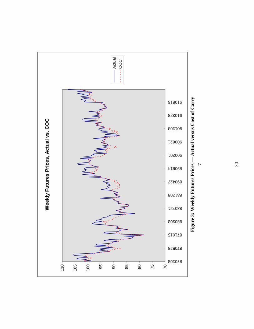
Since the test of the COC model requires data on all deliverable bonds, the test is

done on weekly data. We select Thursday’s prices to be consistent with the Chen and

Scott study (1993).18 We find the cheapest to deliver bond by minimizing B/q for every

given week and then use Eq 24 to compute futures prices. The results of this calculation

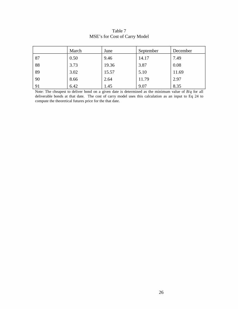
as well as the weekly futures prices from the CBOT are plotted in Figure 3. The MSE is

17 It should be kept in mind that all bonds considered here will potentiall y be the cheapest if the interestrates at maturity settle in its relevant region.18 If Thursday prices are not available, we use Friday’s prices. This selection is also consistent with Chenand Scott (1993) so that the factor values for the model are consistent with the COC model.

17

calculated as 7.8838 for the whole period. The breakdown of each contract is given in

Table 7.

Figure 3: Weekly Futures Prices

Table 7: MSE’s for the Cost of Carry Model

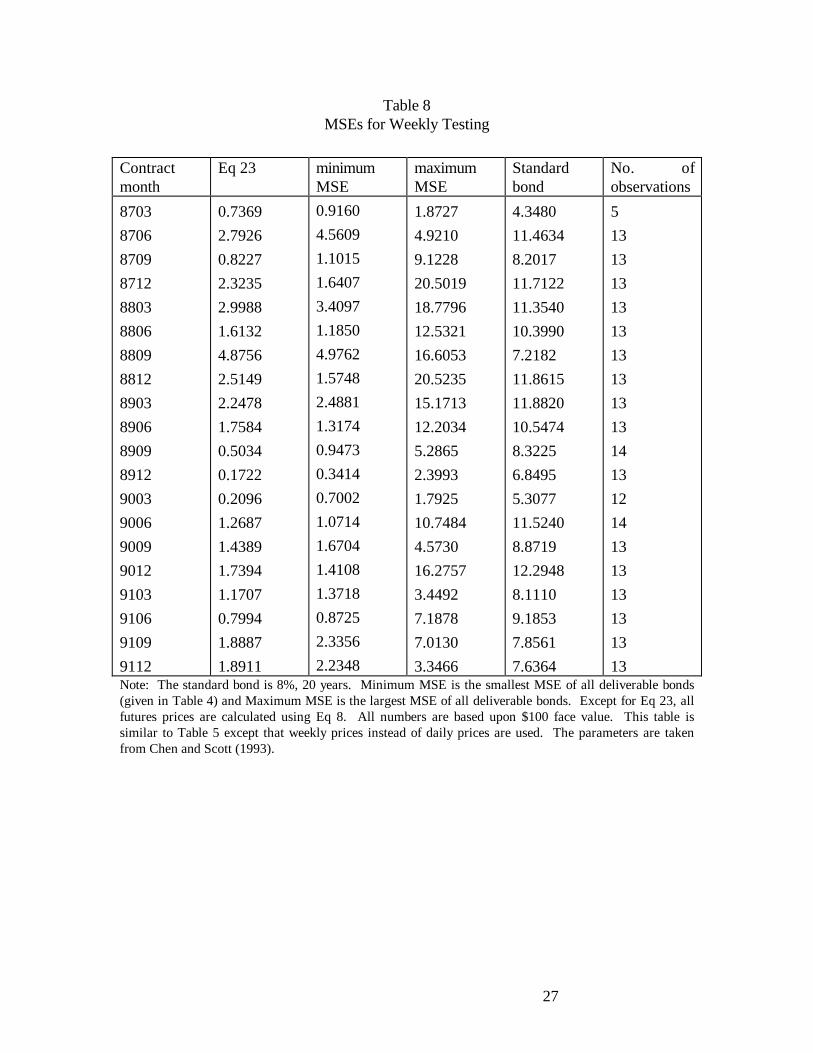
To test our model against the COC model, we need to compute Eq 23 once a week. We

repeat the procedure used to generate Table 5 and the results are given in Table 8. The

MSE of our model for the whole sample period is 1.7197, representing an 80% reduction

in error over the COC model.

Table 8: MSE’s for weekly testing

5 SUMMARY

This paper derives and empirically tests a quality option model which overcomes several

disadvantages of previous models. First, it is consistent with a general equili brium theory

of the term structure. Second, it avoids the use of multi-dimensional bond price processes

which are difficult to implement. Third, it provides closed form solutions in the single

factor case.

The empirical work in this paper is very supportive of the two factor model. The

evidence suggests that the magnitude of the quality option in T-Bond futures contracts is

not trivial. It also shows a significant difference between the two factor CIR model and

the cost of carry model. Further research should focus on parameter estimation of the two

factor model.

APPENDIX

This Appendix finds an expression for the first truncated moment of the terminal adjusted

bond price:

01

28

2r

b

j

bj

p f j j

B r T

qr dr

C

qF r T T B T r v∫ ∑= +

=

(~, )(~) ~ ( , ; ) [ ( ( )) ; , ]*φ χ η Λ

18

We begin by substituting the coupon bond definition into the integral on the left hand side

of the above equation:

0 01

10

10

8 8

8

8

rb

r

j

bj

j

j

b r jj

j

bj

j

r r B T

B r T

qr dr

C

qP r T r dr

C

qP r T r dr

C

qA T e r drj

∫ ∫ ∑

∑ ∫

∑ ∫

=

=

=

=

=

=

−

(~, )(~) ~ (~, ) (~) ~

(~, ) (~) ~

( ) (~) ~~ ( )

φ φ

φ

φ

The integral here is recognized as the truncated Laplace transform of the density function

φ(~)r , evaluated at the point B Tj( ) . Using the density function provided in CIR (1985)

under the square root process:

φ η(~| ) ( )/

r r ev

uI uvu v

q

q=

− −2

2

where:

( )η

ηη

κ λ

σ

κ λ

κµσ

κ λ=

==

= −

+

−

− +

− +2

1

2

2

2 1

( )

( )

( ))

~

e

T

T f

fu e r

v r

q

Iq ( )⋅ is the modified Bessel function of the first kind of order q:

I xx

j q jq

j

q j

( )( / )

! ( )=

+ +=

∞ +

∑0

22

1Γ

Substituting this expression back to the integral yields:

A T e r dr A T e ev

u

uv

j q jdr

A T ev

u

u r

j q jdr

j

r r B T

j

r r B T u vq

j

q j

j

r u B T rq

j

j q j

j j

j

( ) (~) ~ ( )( )

! ( )~

( )( ~)

! ( )~

* *

*

~ ( ) ~ ( )/ /

( ( ))~/

0 0

2

0

2

0

2

0

1

1

∫ ∫ ∑

∫ ∑

− − − −

=

∞ +

− − +

=

∞ +

=

+ +

=

+ +

φ η

η ηη

Γ

Γ

19

In order to represent the integral as the distribution function of a non-central chi-squared

distribution, consider the affine transformation y B T rj= +2( ( ))~η :

[ ]

[ ] [ ]

A T eu

j q j B Tdy

A TB T

e u

j q jdy

C T e

j

B T ru v

j

j yB T

q j

j

jj

q jB T r u v

j

j uB T

jy q j

f

B T r

j j

j j

B Tj u

B Tj j

( )! ( ) ( ( ))

( )( ) ! ( )

( )

( ( )) */ ( ( ))

( ( )) * /( )

( ( )) *( )

( )

ηη

ηη

ηη

η

ηη

η

ηη

0

22

0

2

0

2 2

0

2

0

2

1

1

2

2 1

+ − −

=

∞ +

+

++ − −

=

∞ ++

+

∫ ∑

∫ ∑

+ +⋅

+

=+

+ +

=−

+

Γ

Γ

[ ]

[ ]∫ ∑

∫ ∑

∫ ∑

− − +

=

∞ ++

+

+− −

+=

∞ ++

+−

=

∞

+

+

+

+ +

=+ +

=

e u y

j q jdy

F r T Te u y

j q jdy

F r T Te y

u v

j

j uB T

jq j

q j

p f j

B T rv

qj

j uB T

jq j

j

p f j

B T r

vj

j v

B Tj u

B Tjj

j

uB Tj

j

j

y

/( )

( ( )) */

( )

( ( )) *

/

( )

( )

( )

( )

! ( )2

( , ; )! ( )2

( , ; )

2

0

0

22

10

0

2

20

2 1

2 1

2

2

η

ηη

ηη

ηη

η

η

Γ

Γ

ΛΛ

/

*

! ( / )2

( , ; ) [ ( ( )) ; , ]

2 1

2

2

2

2

+ −

+

= +

j

j

p f j j

j v jdy

F r T T B T r

Γ

Λχ η ν

where v (degrees of freedom) and Λ (non-centrality parameter) are defined in the text.

We complete the proof by substituting this result into the original equation.

20

Table 1Crossover Rates for the One Factor Model

Contract Cheapest Deliverable Bonds

Bond 1 Bond 2

Crossover Rate

8703

8706

8709

8712

8803

8806

8809

8812

8903

8906

8909

8912

9003

9006

9009

9012

9103

9106

9109

9112

9.25, Feb, 2016

7.25, May, 2016

8.875, May, 2018

7.25, May, 2016

8.875, May, 2018

7.25, May, 2016

8.875, May, 2018

7.25, May, 2016

8.875, May, 2018

7.25, May, 2016

8.125, Aug, 2019

7.25, May, 2016

8.125, Aug, 2019

7.25, May, 2016

8.125, Aug, 2019

8.75, May, 2020

7.875, Feb, 2021

8.125, May, 2021

7.875, Feb, 2021

8.125, May, 2021

N.A.

N.A.

N.A.

N.A.

N.A.

N.A.

N.A.

N.A.

N.A.

N.A.

N.A.

N.A.

N.A.

N.A.

N.A.

7.25, May, 2016

N.A.

N.A.

N.A.

N.A.

N.A.

N.A.

N.A.

N.A.

N.A.

N.A.

N.A.

N.A.

N.A.

N.A.

N.A.

N.A.

N.A.

N.A.

N.A.

0.015

N.A.

N.A.

N.A.

N.A.Note: The parameter values used to simulate the crossover rate are the estimates of the one factor CIRmodel in Chen and Scott (1993). Eq 9 is used to calculate various bond prices. The cheapest bond isidentified by minimizing B/q (where q is the conversion factor) across various bonds. Bond 1 is thecheapest bond in the interest rate region lower than the crossover rate and Bond 2 is the cheapest bond inthe interest rate region higher than the crossover rate.

21

Table 2Deliveries in Last Week

Contract Total Last day day -1 day -2 day -3 day -4 day -5

8703 100.00% 70.10% 85.42% 99.98% 99.99% 100.00% 100.00%

8706 100.00% 99.85% 99.85% 99.93% 100.00% 100.00% 100.00%

8709 100.00% 99.44% 99.89% 99.89% 99.89% 99.91% 100.00%

8712 100.00% 65.00% 74.16% 74.16% 74.88% 74.88% 76.50%

8803 100.00% 93.18% 94.62% 97.21% 97.24% 97.24% 97.24%

8806 100.00% 100.00% 100.00% 100.00% 100.00% 100.00% 100.00%

8809 100.00% 99.87% 99.92% 99.92% 100.00% 100.00% 100.00%

8812 100.00% 51.41% 85.10% 85.67% 88.00% 93.59% 94.31%

8903 100.00% 0.01% 0.96% 2.95% 13.45% 15.31% 15.31%

8906 100.00% 21.35% 22.05% 22.05% 22.21% 27.77% 28.16%

8909 100.00% 70.55% 71.15% 73.29% 77.27% 79.89% 79.89%

8912 100.00% 49.24% 94.93% 94.93% 94.93% 96.18% 96.20%

9003 100.00% 99.89% 99.89% 100.00% 100.00% 100.00% 100.00%

9006 100.00% 97.42% 99.86% 99.86% 99.87% 99.93% 99.93%

9009 100.00% 87.14% 99.99% 100.00% 100.00% 100.00% 100.00%

9012 100.00% 1.92% 1.92% 4.05% 4.05% 4.13% 4.13%

9103 100.00% 96.58% 99.90% 99.94% 100.00% 100.00% 100.00%

9106 100.00% 98.29% 100.00% 100.00% 100.00% 100.00% 100.00%

9109 100.00% 99.83% 99.94% 99.94% 99.94% 99.96% 100.00%

9112 100.00% 99.13% 99.59% 99.83% 99.83% 99.83% 99.83%Note: The percentage numbers are cumulative actual deli veries from the last day in the deli verymonth. The “Last day” column presents the deli veries in the last day of the deli very month as apercentage of total deli veries in the deli very month. The “day -1” column is the deli veries for thelast two days of the deli very month as a percentage of the total. The remaining columns show thecumulative (backwards) quantities of actual deli veries in the deli very month. For example, forcontract 8703, the deli very month is March, 1987. The last day in that month is 31st, a Tuesday.On that day, 7 issues are deli vered, totaling 11014 bond contracts and representing 70.10% oftotal deli veries in March, 1987, which is 14428. On day -1, which is the 30th, 4 issues of 2210contracts are deli vered, representing 15.32% of the total. Therefore, the cumulative percentage fortwo days is 85.42%.

22

Table 3Summary Statistics of Daily Futures Prices from 1/87 till 12/91

N Mean Std Dev Min Max

All maturities

8703

8706

8709

8712

8803

8806

8809

8812

8903

8906

8909

8912

9003

9006

9009

9012

9103

9106

9109

9112

1275

21

63

64

65

63

64

64

65

63

64

64

65

63

64

64

65

63

64

63

64

92.65

100.62

97.23

90.72

84.59

88.23

91.19

86.68

87.53

89.09

88.73

95.23

97.42

98.29

92.26

93.15

89.60

94.91

95.95

93.83

98.17

4.7686

0.6833

3.2328

1.5606

3.3369

2.1470

1.9662

1.2191

2.1673

1.1461

1.0879

3.1389

1.1772

1.9000

1.6765

1.1783

1.2881

1.6509

1.1031

0.9250

1.4522

77.78

99.47

88.56

86.84

77.78

83.72

97.34

84.44

83.94

86.97

86.50

88.34

95.25

93.22

88.59

89.78

87.16

91.09

93.44

92.28

95.25

104.75

101.59

101.38

93.19

90.09

93.91

94.16

89.56

91.41

91.44

91.28

100.38

99.84

100.28

94.72

95.19

93.09

97.56

97.94

95.94

100.41Note: The face value of the underlying bond is assumed to be $100.

23

Table 4Possible Deliverable Bonds

Contract Bond 1 Bond 2 Bond 3 Bond 4 Bond 5

8703

8706

8709

8712

8803

8806

8809

8812

8903

8906

8909

8912

9003

9006

9009

9012

9103

9106

9109

9112

10.75,2,03

11.625,11,0

2

10.75,2,03

10.75,2,03

11.125,8,03

11.875,11,0

3

13.75,8,04

12.3755,04

13.75,8,04

7.875,11,02

8.375,8,03

7.875,11,02

10.75,2,05

12.75,11,05

9.375,2,06

13.875,5,06

12,8,08

14,11,06

12,8,08

14,11,06

8.375,8,03

7.875,11,02

8.375,8,03

7.875,11,02

8.375,8,03

7.875,11,02

8.375,8,03

7.875,11,02

8.375,8,03

8.25,5,05

7.625,2,07

8.25,5,05

7.625,2,07

10.375,11,0

7

7.625,2,07

10.375,11,0

7

7.625,2,07

10.375,11,0

7

7.625,2,07

10.375,11,0

7

7.625,2,07

8.25,5,05

7.625,2,07

8.25,5,05

7.625,2,07

8.25,5,05

7.625,2,07

8.25,5,05

7.625,2,07

7.25,5,16

9.25,2,16

7.25,5,16

9.25,2,16

7.25,5,16

9.25,5,16

7.25,5,16

9.25,2,16

7.25,5,16

9.25,2,16

7.25,5,16

9.25,2,16

7.25,5,16

8.875,8,17

7.25,5,16

9.25,2,16

7.25,5,16

9.25,2,16

7.25,5,16

9.25,2,16

8.875,8,17

8.125,8,19

8.125,8,19

8.875,8,17

8.125,8,19

8.875,8,17

8.875,8,17

8.875,8,17

8.125,8,19

8.125,8,19

7.875,2,21

Note: These bonds are the possible deli verable bonds for each contract. The table is similar to Table 1except that a two factor version of Eq 9, i.e., Eq 9 with Eq 20, is used. All bonds are reported by theircoupons (first number) and maturity month (second number), and maturity year (third number).

24

Table 5MSEs for Daily Testing

Contractmonth

Eq 23 MinimumMSE

MaximumMSE

Standardbond

No. ofobservations

8703

8706

8709

8712

8803

8806

8809

8812

8903

8906

8909

8912

9003

9006

9009

9012

9103

9106

9109

9112

49.7002

26.8069

7.4268

3.4922

3.7274

3.2481

3.0263

1.3520

0.8782

3.4598

5.4144

3.2872

2.7328

2.8513

1.8728

3.3684

3.8978

2.4051

2.5173

1.5190

50.7703

31.8355

8.1547

3.5766

4.0159

3.0677

3.1512

0.8502

0.9223

3.4136

2.1401

3.6892

0.5997

2.7955

1.7265

3.3324

1.9298

2.4568

2.7798

1.8175

79.1000

42.1938

18.3405

13.4459

17.1279

13.7105

21.1838

15.9503

9.8478

5.1505

4.8693

3.9476

2.3080

5.3054

2.7025

8.8694

3.6592

7.3579

6.4933

3.2730

78.7916

46.6872

17.3513

10.3625

12.7534

11.5997

11.6031

9.7288

7.3389

6.3542

5.5764

8.3660

5.1455

6.7327

6.4281

7.6758

6.1190

9.4754

9.0371

7.7540

22

63

64

65

63

64

64

65

63

64

64

65

63

64

64

65

63

64

63

64Note: The standard bond is 8%, 20 years. Minimum MSE is the smallest MSE of all deli verable bonds(given in Table 4) and Maximum MSE is the largest MSE of all deli verable bonds. Except for the columnlabeled Eq 23, all futures prices are calculated using Eq 8. All numbers are based upon $100 face value.The parameter values used are the estimates of the two factor CIR model provided by Chen and Scott(1993).

25

Table 6MSE’s for Daily Testing with Constantly Updated σ 2

2

March June September December

87

88

89

90

91

13.74

0.68

0.31

0.29

0.55

0.77

0.48

0.72

0.82

0.23

0.85

0.53

0.91

0.71

0.24

1.27

0.27

0.58

1.18

0.32Note: The MSE’s reported are calculated the same way as Eq 23 in Table 5 except that the volatilit yparameter σ is updated daily. We use the implied σ for the next day’s futures price calculation.

26

Table 7MSE’s for Cost of Carry Model

March June September December

87

88

89

90

91

0.50

3.73

3.02

8.66

6.42

9.46

19.36

15.57

2.64

1.45

14.17

3.87

5.10

11.79

9.07

7.49

0.08

11.69

2.97

8.35Note: The cheapest to deli ver bond on a given date is determined as the minimum value of B/q for alldeli verable bonds at that date. The cost of carry model uses this calculation as an input to Eq 24 tocompute the theoretical futures price for the that date.

27

Table 8MSEs for Weekly Testing

Contractmonth

Eq 23 minimumMSE

maximumMSE

Standardbond

No. ofobservations

8703

8706

8709

8712

8803

8806

8809

8812

8903

8906

8909

8912

9003

9006

9009

9012

9103

9106

9109

9112

0.7369

2.7926

0.8227

2.3235

2.9988

1.6132

4.8756

2.5149

2.2478

1.7584

0.5034

0.1722

0.2096

1.2687

1.4389

1.7394

1.1707

0.7994

1.8887

1.8911

0.9160

4.5609

1.1015

1.6407

3.4097

1.1850

4.9762

1.5748

2.4881

1.3174

0.9473

0.3414

0.7002

1.0714

1.6704

1.4108

1.3718

0.8725

2.3356

2.2348

1.8727

4.9210

9.1228

20.5019

18.7796

12.5321

16.6053

20.5235

15.1713

12.2034

5.2865

2.3993

1.7925

10.7484

4.5730

16.2757

3.4492

7.1878

7.0130

3.3466

4.3480

11.4634

8.2017

11.7122

11.3540

10.3990

7.2182

11.8615

11.8820

10.5474

8.3225

6.8495

5.3077

11.5240

8.8719

12.2948

8.1110

9.1853

7.8561

7.6364

5

13

13

13

13

13

13

13

13

13

14

13

12

14

13

13

13

13

13

13Note: The standard bond is 8%, 20 years. Minimum MSE is the smallest MSE of all deli verable bonds(given in Table 4) and Maximum MSE is the largest MSE of all deli verable bonds. Except for Eq 23, allfutures prices are calculated using Eq 8. All numbers are based upon $100 face value. This table issimilar to Table 5 except that weekly prices instead of dail y prices are used. The parameters are takenfrom Chen and Scott (1993).

28

Cro

sso

ver

Rat

es

020406080100

120

140

160

180

0

0.02

0.04

0.06

0.08

0.1

0.12

0.14

0.16

0.18

0.2

0.22

0.24

0.26

0.28

0.3

yiel

d

price

8%, 1

0-yr

6%, 5

-yr

7%, 3

-yr

chea

pest

Fig

ure

1: T

hree

Adj

uste

d B

ond

Pric

es C

ross

ing

Tw

ice

29

Dai

ly (

Act

ual

) F

utu

res

Pri

ces

707580859095100

105

870102

870316

870527

870805

871015

871224

880308

880518

880729

881007

881215

890228

890510

890721

890929

891207

900220

900502

900713

900921

901129

910211

910424

910705

910916

911125

Fig

ure

2: D

aily

Fut

ures

Pric

es —

Act

ual

30

Wee

kly

Fu

ture

s P

rice

s, A

ctu

al v

s. C

OC

707580859095100

105

110

870108

870528

871015

880303

880721

881208

890427

890914

900201

900621

901108

910328

910815

Act

ual

CO

C

Fig

ure

3: W

eekl

y F

utur

es P

rices

— A

ctua

l ver

sus

Cos

t of C

arry

7

31

REFERENCES

Bick, A., 1996, “Two Closed Form Formulas for the Futures Price in the Presence of the

Quality Option,” working paper, Simon Fraser University.

Chowdry, B., 1986, “Pricing of Futures with Quality Option,” Working paper, University

of Chicago.

Boyle, P., 1989 (March),“The Quality Option and Timing Option in Futures Contracts,”

Journal of Finance, Vol. 44, No. 1.

Brennan, M. and E. Schwartz, 1979 (July), “A Continuous Time Approach to the Pricing

of Bonds,” Journal of Banking and Finance.

Chen, R. and L. Scott, 1992, “Pricing Interest Rate Options in a Two Factor Cox-

Ingersoll-Ross Model of the Term Structure,” Review of Financial Studies, Vol. 5,

No. 4, pp. 613-636.

Chen, R. and L. Scott, 1993, “Maximum Likelihood Estimation of a Multi-Factor

Equili brium Model of the Term Structure of Interest Rates,” Journal of Fixed

Income.

Chen, R. and L. Scott, 1995, “Multi-Factor Cox-Ingersoll-Ross Models of the Term

Structure: Estimates and Tests from a Kalman Filter Model,” working paper,

Rutgers University.

Cheng, S., 1985, “Multiple Factor Contingent Claims in a Stochastic Interest Rate

Environment,” Working paper, Columbia University.

Cherubini, U. and M. Espesito, 1996, “Options In and On Interest Rate Futures Contracts:

Results from Martingale Pricing Theory.”

Courtadon, G., 1982, “The Pricing of Options on Default-Free Bonds,” Journal of

Financial and Quantitative Analysis.

Cox, J., J. Ingersoll, and S. Ross, 1985 (March), “A Theory of The Term Structure of

Interest Rates,” Econometrica.

Cox, J., J. Ingersoll, and S. Ross, 1981, “The Relation Between Forward Prices and

Futures Prices,” Journal of Financial Economics, p.321-346.

Duan, J. and J. Simonato, 1995, “Estimating and Testing Exponential-Affine Term

Structure Models by Kalman Filter,” working paper, McGill University.

Duffie, D. and R. Kan, 1992, “A Yield Factor Model of Interest Rates,” working paper,

Stanford University.

Gibbons, M. and K. Ramaswamy, 1993, “A Test of the Cox, Ingersoll, and Ross Model of

the Term Structure,” Review of Financial Studies.

32

Flesaker, B. and L. Hughston, 1996 (January), “Positive Interest,” RISK, Vol. 9 No. 1, pp.

46-49.

Hemler, M., 1990 (December), “The Quality Delivery Option in Treasury Bond Futures

Contracts,” Journal of Finance, Vol. 45, No. 5.

Heston, S., 1989, “Testing Continuous Time Models of the Term Structure of Interest

Rates: A New Methodology for Contingent Claim Valuation,” Working paper,

Carnegie Mellon University.

Jamshidian, F., 1993, “Bond, Futures and Option Evaluation in the Quadratic Interest

Rate Model'', working paper, Fuji International Fiannce.

Kane, A. and A. Marcus, 1986 (Summer), “The Quality Option in the Treasury Bond

Futures Contract: An Empirical Assessment,” Journal of Futures Markets, Vol. 6.

Longstaff, F. and E. Schwartz, 1992 (September), “Interest Rate Volatili ty and the Term

Structure: A Two Factor General Equili brium Model,” Journal of Finance, V.46,

No.4, p.1259-1282.

Lund, J., 1994, “Econometric Analysis of Continuous Time Arbitrage Free Models of the

Term Structure of Interest Rates,” working paper, Aarhus Business School.

Pearson, N. and T. Sun, 1994 (September), “Exploiting the Conditional Density in

Estimating the Term Structure: An Application to the Cox, Ingersoll, and Ross

Model,” Journal of Finance, p.1279-1304

Richard, S., 1978, “An Arbitrage Model of the Term Structure of Interest Rates,” Journal

of Financial Economics.

Ritchken, P. and L. Sankarasubramanian, 1992, (July), “Pricing the Quality Option in

Treasury Bond Futures,” Mathematical Finance, V.2, No.3, p.197-214.

Vasicek, O., 1977, “An Equili brium Characterization of the Term Structure,” Journal of

Financial Economics, November.