Values in the Wind: A Hedonic Analysis of

Wind Power Facilities∗

Martin D. Heintzelman

Carrie M. Tuttle

March 3, 2011

Economics and Financial Studies

School of Business

Clarkson University

E-mail: mheintze@clarkson.edu

Phone: (315) 268-6427

∗Martin D. Heintzelman is Assistant Professor, Clarkson University School of Business.Carrie M. Tuttle is a Ph.D. Candidate in Environmental Science and Engineering at ClarksonUniversity. We would like to thank Michael R. Moore, Noelwah Netusil, and seminar par-ticipants at Binghamton University as well as the 2010 Thousand Islands Energy ResearchForum and the 2010 Heartland Economics Conference for useful thoughts and feedback. Allerrors are our own.

1

ABSTRACT: The siting of wind facilities is extremely controversial. This

paper uses data on 11,369 property transactions over 9 years in Northern New

York to explore the effects of new wind facilities on property values. We use

a repeat-sales framework to control for omitted variables and endogeneity bi-

ases. We find that nearby wind facilities significantly reduce property values.

Decreasing the distance to the nearest turbine to 1 mile results in a decline

in price of between 7.73% and 14.87%. These results indicate that there re-

mains a need to compensate local homeowners/communities for allowing wind

development within their borders.

2

1 Introduction

Increased focus on the impending effects of climate change has resulted in

pressure to develop additional renewable power supplies, including solar, wind,

geothermal, and other sources. While renewable power provides several envi-

ronmental advantages to traditional fossil fuel supplies, there remain signifi-

cant obstacles to large-scale development of these resources. First, most re-

newable energy sources are not yet cost competitive with traditional sources.

Second, many potential renewable sources are located in areas with limited

transmission capacity, so that, in addition to the costs of individual projects,

large-scale development would also require major infrastructure investments.

Finally, renewable power projects are often subject to local resistance.

Wind power is, by far, the fastest growing energy source for electricity

generation in the United States, capacity and net generation having increased

by more than 1,348% and 1,164%, respectively, between 2000 and 2009. No

other sources of electricity have even doubled in capacity over that period.

This sort of growth for wind energy is expected to continue into the future,

although not at quite those high rates.1 If additional steps are taken to combat

global climate change, the demand for wind energy would only increase relative

to these forecasts.

There are many outspoken critics who focus on the potential negative im-

pacts of wind projects. These critics point to the endangerment of wildlife

including bats, migratory birds, and even terrestrial mammals. Some critics

also point to detrimental human health effects including abnormal heartbeat,

insomnia, headaches, tinnitus, nausea, visual blurring, and panic attacks.2

3

There are also more mundane concerns about the aesthetics of these facilities.

One oft-quoted critic, Hans-Joachim Mengel a Professor of Political Science

at the Free University, Berlin, has likened Wind Turbines to “the worst dese-

cration of our countryside since it was laid waste in the 30 Years War nearly

400 years ago.”3 If wind turbines are perceived to have this manner of impact

on local areas, they would have a strong negative impact on local property

values.

To give an idea of how far-reaching we might expect the impacts to be,

consider that estimated sound levels for a typical turbine at a distance of

1500 ft. are 50 dBA, equivalent to a normal indoor home sound level (Colby

et al., 2009). In comparison, the Occupational Safety and Health Adminis-

tration (OSHA) requires that sound levels for prolonged unprotected occu-

pational exposures be less than 90 dBA. This exposure would be equivalent

to standing next to a highway with heavy diesel trucks passing by for an 8-

hour time period.4 Typically, distances between wind turbines and receptors

are regulated at the local level. The New York State Energy Research and

Development Authority (NYSERDA) recommends turbine setbacks of 1000

ft. from the nearest residence (Daniels, 2005). These setbacks focus on gen-

eral safety considerations such as turbine collapse instead of specific health

impacts associated with noise or vibration. The National Environmental Pro-

tection Act and comparable New York State Environmental Quality Review

legislation prescribe a general assessment process that does not define specific

turbine setback requirements. Viewshed impacts are more far reaching but

vary widely by property and depend on land cover and property elevations.

4

As a result of these potential effects, the siting of wind facilities is extremely

controversial, and debate about siting has caused delays and cancellations for

some proposed installations. Perhaps the most famous case is that of Cape

Wind in Massachusetts. First proposed in 2001, this project, approved by the

U.S. Department of Interior in April 2010, calls for the construction of 130

turbines, each with a maximum blade height of 440 ft., approximately 5 miles

off the shore of Cape Cod between Cape Cod and Nantucket. In response,

local activists have organized the “Alliance to Protect Nantucket Sound” to

fight the proposal through the courts and other avenues. This is despite the

fact that the primary local impact is expected to be the impacted view from

waterfront properties.5 In the case of terrestrial projects, the opposition can

be even stronger. In Cape Vincent, NY, in Jefferson County, wind developers

have been working since 2006 to construct two separate facilities that include

147 turbines. Cape Vincent is bordered to the north by the St. Lawrence

River and Lake Ontario, within view of an eighty-six turbine wind farm on

Wolf Island in Ontario, Canada, and within a short drive to the largest wind

farm in New York State. The response to the proposal has been spirited with

both pro- and anti-wind factions fighting to determine its fate. In October

of 2010, a lawsuit was filed to nullify a town planning board’s approval of a

final environmental impact statement; the meeting at which it was approved

had been disrupted by vocal protestors.6 Recent reports in the popular media

suggest that such controversy over wind turbines is widespread.7

At the individual level, property owners willing to permit the construction

of turbines or transmission facilities on their property receive direct payments

5

from the developer as negotiated through easement agreements. In terms of

community benefits, wind developers claim that their projects create jobs and

increase tax revenues by way of payment in lieu of taxes (PILOT) programs.

PILOTs are a significant revenue source that can help offset overall town and

school tax rates for all residents. These host community benefits are not

unlike those made to communities that have permitted the construction of

landfills within their municipal boundaries. In the case of Cape Vincent, a

town appointed committee evaluated the economic impacts of the proposed

facility and concluded that 3.9% of property owners would benefit directly

from easement payments made by the developers.8 Easement payments are

negotiated with individual land owners and are not publically available so

the magnitude and actual economic benefit to these property owners was not

quantified. PILOT agreements between the developers and the Town were

estimated at $8,000 per turbine or $1.17 million per year. In the opinion

of some Cape Vincent property owners, local officials are negotiating PILOT

agreements to the benefit of the municipality, individual property owners are

negotiating individual easement agreements to offset their respective property

impacts, and property owners in close proximity to turbines are left with no

market leverage to offset the impacts that they believe turbines will have on

their property values. This is the externality problem that is at the heart of

the issue.

In moving forward with wind power development then, it is important to

understand the costs that such development might impose. Unlike traditional

energy sources, where external/environmental costs are spread over a large

6

geographic area through the transport of pollutants, the costs of wind devel-

opment are largely, but not exclusively, borne by local residents. Only local

residents are likely to be negatively affected by any health impacts, and are

the people who would be most impacted by aesthetic damages, either visual or

audible. These impacts are likely to be capitalized into property values and,

as a consequence, property values are likely to be a reasonable measuring stick

of the imposed external costs of wind development.

The literature that attempts to measure these costs is surprisingly thin.

To our knowledge, there are only two peer-reviewed hedonic analyses that

examine the impact of wind power facilities on property values. Sims et al.

(2008) and Sims et al. (2007) use small samples of homes near relatively small

wind facilities near Cornwall, UK and find no significant effect of turbines on

property values. The first of these studies has very limited data on homes, just

home ‘type’ and price, and uses a cross-sectional approach. In addition, there is

a quarry adjacent to the wind turbines, and other covarying property attributes

which makes identification of the wind turbine effect very difficult. They

actually do find a significant negative effect from proximity to the turbines

but based on conversations with selling agents, attribute this instead to the

condition and type of the homes. The second study uses a very small sample of

only 201 homes all within the same subdivision and a cross-sectional approach.

They focus specifically on whether homes can view the turbines and have very

limited data on home attributes. Moreover, given the small geographic scope

of the analysis, it is unlikely that there was sufficient variation in the sample

to identify any effect; all of the homes were within 1 mile of the turbines.

7

In 2003, Sterzinger et al. released a report through the Renewable Energy

Policy Project (REPP) which used a series of 10 case studies to compare price

trends between turbine viewsheds and comparable nearby regions and found,

in general, that turbines did not appear to be harming property values. This

analysis, however, was not a true hedonic analysis. Instead, for each project

they identified treated property transactions as being within a 5 mile radius of

the home and a group of comparable control transactions outside of that range.

They then calculated monthly average prices, regressed these average prices on

time to establish trends and then compared these trends between treatment

and control groups. They did not control for individual home characteristics

or any other coincident factors.

Hoen (2006) also focuses on the view of wind turbines, and collects data for

homes within 5 miles of turbines in Madison County, NY. His sample is also

small, 280 transactions spread over 9.5 years, and he uses a cross-sectional ap-

proach. He fails to find a significant impact from homes being within viewing

range of the turbines. Hoen et. al (2009) use a larger sample of 7,500 homes

spread over 24 different regions across the country from Washington to Texas

to New York that contain wind facilities and again find no significant effect.

They look at transactions within 10 miles of wind facilities and use a variety of

approaches, including repeat sales. However, they limit themselves to discon-

tinuous measures of proximity based on having turbines within 1 mile, between

1 and 5 miles, or outside of 5 miles, or a similar set of measures of the impact

on scenic view, and they again find no adverse impacts from wind turbines. In

addition, by including so many disparate regions within one sample they may

8

be missing effects that would be significant in one region or another.

There is also a small literature using stated preference approaches to value

wind turbine disamenities. Groothuis, Groothuis, and Whitehead (2008) asked

survey respondents about the impact of locating wind turbines on Western

North Carolina ridgetops and found that on average households are willing-

to-accept compensation of $23 to allow for wind turbines, although retirees

moving into the area require greater compensation. Similarly, Krueger, Par-

sons, and Firestone (2011) surveyed Delaware residents about offshore wind

turbines and find that residents would be harmed by between $0 and $80 de-

pending on where the turbines are located and whether the resident lives on

the shore or inland.

This paper improves upon this literature using data on 11,369 arms-length

residential and agricultural property transactions between 2000 and 2009 in

Clinton, Franklin, and Lewis Counties in Northern New York to explore the

effects of relatively new wind facilities. We use a repeat-sales fixed effects

analysis to control for the omitted variables and endogeneity biases common

in hedonic analyses, including the previous literature on the impacts of wind

turbines. We find that nearby wind facilities significantly reduce property

values. To be specific, decreasing the distance to the nearest turbine to 1

mile results in a decline in price of between 7.73% and 14.87% on average. In

addition we confirm that census block-group fixed effects models are subject to

endogeneity bias and that this bias inflates the negative impacts of turbines on

property values by about 35%. These results are consistent across continuous

functional specifications of the proximity effect. However, attempts to control

9

for dis-continuities through a series of dummy and count variables representing

the presence of turbines at various distances are insignificant.

Section 2 provides background information on wind development and on

the study area. Section 3 provides detailed information on our data and em-

pirical approach. Section 4 provides analytical results and Section 5 concludes

the paper by discussing the implications of our study and guidance for further

research in this area.

2 Background and Study Area

New York State is a leader in wind power development. In 1999, New York had

0 MW of installed wind capacity, but by 2009 had 14 existing facilities with

a combined capacity of nearly 1300 MW, ranking it in the top 10 of states in

terms of installed capacity.9 New York also appears to have more potential for

terrestrial wind development than any other state on the east coast.10 This is

borne out by the fact that there are an additional 28 wind projects in various

stages of proposal/approval/installation in the state. 11

New York has also been badly affected by the environmental impacts of

traditional energy sources. The Adirondack Park, the largest park of its sort in

the country, in particular, has been severely impacted by acid deposition and

methyl mercury pollution (Banzhaf et al., 2006). In that sense, the state has

much to gain from transitioning away from fossil sources of energy and towards

renewable sources like wind. New York, however, has relatively little potential

to develop solar, geothermal, or other renewable sources. Existing wind devel-

10

opments are spread throughout the state, with clusters in the far west, the far

north, and in the northern finger lakes region. The largest projects, however,

are in what is often referred to as ‘The North Country,’ and are in the three

counties - Clinton, Franklin and Lewis Counties - which make up our study

area, shown in Figure 1, together with the outline of the Adirondack Park and

the location of the wind turbines in this area.

Northern New York is dominated by the presence of the Adirondack Park.

The Adirondack Park was established in 1892 by the State of New York to

protect valuable natural resources. Containing 6.1 million acres, 30,000 miles

of rivers and streams, and over 3,000 lakes, the Adirondack Park is the largest

publically protected area in the United States and is larger than Yellowstone,

Everglades, Glacier, and Grand Canyon National Park combined. Approxi-

mately 43% of the Park is publically owned and constitutionally protected to

remain “forever wild” forest preserve. The remaining acreage is made of up

private land holdings. There are no wind facilities within the borders of the

Park, but as you can see in Figure 2, the facilities in our study are very close.

There are six wind farms in our study area, as summarized in Table 1.12

Table 2 presents a comparison of the counties in our study area to the

New York State and United States averages for population density and per

capita income. As that table shows, our study area is a very rural, lightly

populated area of small towns and villages that is also less affluent than the

state average. The largest population center in our study area is Plattsburgh,

NY with a 2000 population of about 18,000.

11

3 Data and Methodology

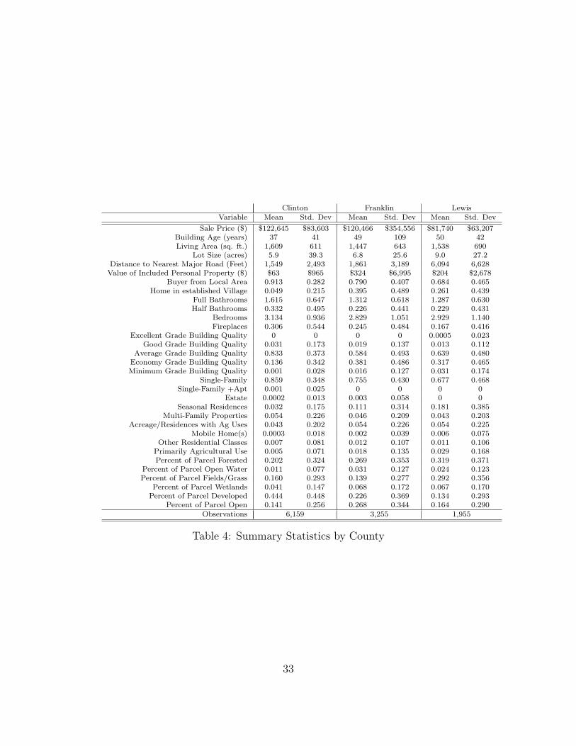
Our data consists of a nearly complete sample of 11,369 residential and agri-

cultural property transactions in the Clinton, Franklin and Lewis Counties

from 2000-2009. Of these there are 1,955 from Lewis, 3,255 from Franklin,

and 6,159 from Clinton counties. Each observation constitutes an arms-length

property sale in one of the three counties between 2000 and 2009. Parcels that

transacted more than once provide a greater likelihood of observing specific

effects from the turbines on sales prior to and after installation. In total, 3,890

transactions occurred for 1,903 parcels that sold more than once during the

study period.

Transacted parcels were mapped in GIS to enable us to calculate relevant

geographic variables for use in the regressions. Turbine locations were obtained

from two different sources. In Lewis County, a GIS shapefile was provided by

the County which contained 194 turbines. According to published information

on the Maple Ridge wind project, there are 195 turbines at the facility (Maple

Ridge Wind Farm). Noble Environmental Power would not provide any infor-

mation on their turbine locations so 2009 orthoimagery was utilized to create

a GIS shapefile with the turbine locations in Franklin and Clinton counties.

Turbine locations in combination with several other datasets were merged

using ESRI ArcView GIS software and STATA data analysis and statistical

software to form the final dataset. Transacted parcels were mapped in GIS to

determine the distance to the nearest turbine. Then buffers, ranging in size

from 0.1 to 3.0 miles, were created around each parcel polygon and these were

spatially joined with the turbine point data to compute the number of turbines

12

located within these various distances from the parcels. Buffer distances are

used as a proxy to estimate the nuisance effects of the turbines (i.e., view-

scapes and noise impacts). The distance to turbines and number of turbines

by parcel were exported from GIS and combined with the other parcel level

details in STATA. Table 3 summarizes the datasets that were used in the

analysis and their sources. Table 4 provides summary statistics for many of

the variables included in our analysis.

3.1 Methodology

Our analytical approach to estimating the effects of wind turbines on property

values is that of a repeat sales fixed-effects hedonic analysis. We are attempting

to estimate the ‘treatment’ effect of a parcel’s proximity to a wind turbine.

There are a number of difficulties in measuring the effect of turbines. First

and foremost, there is a question of when a turbine should be said to ‘exist.’

The obvious answer is that turbines exist only after the date on which they

become operational. However, there is a long approval process associated with

development of these projects and local homeowners presumably will have

some information about where turbines will be located some years before they

actually become operational. To deal with this issue, we run our regressions

with three different assumptions about the date of existence - the date the

draft environmental impact statement was submitted to the New York State

Department of Environmental Conservation, the date the final environmental

impact statement was approved, and the date at which the turbines became

operational.

13

In addition, given the uncertain and possibly diverse physical/aesthetic

impacts of turbines, it is difficult to know how to measure proximity. Is it

distance to the turbine, whether or not the turbine can be seen, whether or

not the turbine can be heard/felt, or all of the above? For all of these factors,

it is reasonable to suspect that distance would work as a proxy measure. That

is, homes closer to turbines will be more likely to see the turbines and more

likely to hear or feel vibrations from the turbines. So, all of the measures that

we employ will be distance based, starting with the simplest - the inverse of

the distance to the nearest turbine.13 This inverse distance measure is also

calculated with the date of the turbines’ existence in mind. So, distance will

decrease (inverse distance will increase) for all parcels after new turbines come

into existence. Unlike some of the previous studies of these effects, we are

dealing with very large facilities, so that if a parcel is near at least one turbine

it is likely near many turbines. To account for this, we employ simple dummy

variables for the presence of at least one turbine within various distances from

the parcel as well as count variables for the number of turbines within those

distances. This enables us to test for any ‘density’ effects. These variables

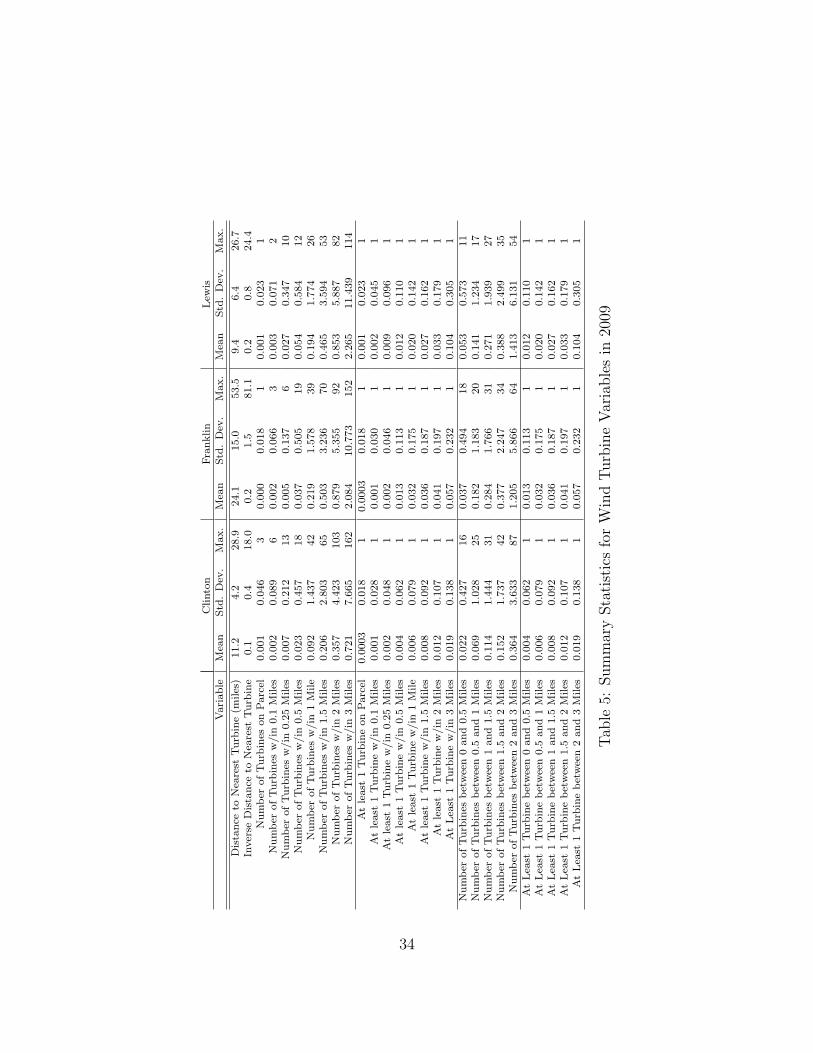
also potentially change over time as new turbines are sited. Table 5 presents

summary statistics for the various measures of the effect of wind turbines that

we employ.

In addition to these various measures of the proximity of homes to wind

turbines, we include a number of other covariates. These include distance

to the nearest major road, the value of any personal property included in

the transaction, whether or not the home is in a ‘village,’ which would im-

14

ply higher taxes, but also higher services and proximity to retail stores and

restaurants, in addition to standard home characteristics including number of

bedrooms, bathrooms, half-baths, the square footage of the house, the age

of the home, and the size of the lot. We also include parcel level land cover

data which tells us the share of each parcel in a number of different land cover

categories (woodland, pasture, crops, water, etc.). To capture possible infor-

mation asymmetries between buyers and sellers we include a dummy variable

for whether or not the buyer was already a local resident or moving in from

outside of ‘the North Country.’ This is particularly important since there is

good reason to believe that local residents would have more information about

the future location of turbines, and about any associated disamenities than

someone moving into the area. Finally we include a series of relatively sub-

jective measures of construction quality and property classification (mobile

homes, primary agriculture, whether or not the home is winterized, etc.) that

come from the NYSORPS (New York State Office of Real Property Services)

assessment database.

3.1.1 Empirical Issues

As Greenstone and Gayer (2009), amongst others, lay out, omitted variables

bias is a major concern in any hedonic analysis. Put simply, there are almost

innumerable factors that co-determine the price of a property, and many or

most of these factors are unobservable to the researcher. If any of the un-

observed factors are also correlated with included factors, then the resulting

coefficient estimates will be biased. Fixed effects analysis, by implicitly in-

15

cluding a large series of dummy variables representing small geographic areas,

or, better yet, individual parcels, captures the effects of any of these unob-

served factors that are constant or similar across the geographic scale of the

fixed effects. For instance, if homes in a particular census block are especially

attractive because of some unobservable factor then the fixed effects analysis

would implicitly pick up the effect of this amenity on the price of homes in

that census block.

The smaller the geographic scale of the fixed effects, the tighter the controls

will be for omitted variables bias. The tradeoff, however, is that since variation

in the remaining observable explanatory variables can only be observed within

the scale of the fixed effects, a smaller geographic scale means less variation

and less power with which to estimate these remaining coefficients. That is, if

we are interested in the distance from each parcel to the nearest major road,

the statistical power to measure this comes only from variation in this distance

within the scope of the fixed effects (ie. the census block). Presumably, since

homes within a census block are all close to each other, they will all be a

similar distance to the nearest road and thus there is limited variation with

which to measure this effect. In a repeat sales analysis, since parcel location

and most other characteristics are assumed to be fixed, one can only estimate

the effects of time-variant factors. However, this level of analysis provides the

cleanest measures of these effects.14

Equally concerning in attempting to accurately estimate the effects of a

discrete change in landscape, like the construction of a wind turbine, is en-

dogeneity bias. This bias has a similar effect as omitted variables bias but a

16

slightly different cause. Endogeneity bias enters when the values of the depen-

dent and one or more independent variables are co-determined. In the case

of hedonic models, if property values determine the location of some facility,

and that facility also impacts property values, we have endogeneity bias. In

our case we do need to be concerned about this since it is likely that, ceteris

paribus, wind turbines will be sited on lower-value, cheaper land. Then, if

this is not corrected, we might falsely conclude that wind turbines negatively

impact property values or, at least, overstate any negative impacts, simply

because wind turbines are placed on cheaper land. This selection effect would

cause us to confuse correlation with causation.

To control for these selection effects we use repeat sales, parcel level, fixed

effects analysis. While census block level fixed effects will do something to

control for this effect since lower value census blocks will be more attractive

for the siting of turbines, if selection of sites for affordability occurs within

census blocks, that is, if the cheapest parcels within a block are more likely

to have or be near a turbine, then endogeneity bias would still be present.

Therefore, the best available correction for endogeneity is parcel-level fixed

effects. If there is some characteristic of a parcel that makes it cheaper, and

that makes it attractive for turbines, the parcel-level fixed effects control for

this selection effect.15

Finally, we have to be concerned about spatial dependence and spatial

autocorrelation. There is no doubt that homes that are close to each other

affect each other’s prices (spatial dependence) and that unobserved factors

for one home are likely to be correlated with unobserved factors for nearby

17

homes (spatial autocorrelation). Both of these factors would bias our results

if not corrected. We correct for these issues using fixed effects, again, for the

first and error clustering for the second. The fixed effects analysis is akin to

employing a spatial lag model with a spatial weights matrix of ones for pairs of

parcels within the same geographic area, the scale of the fixed effects, and zeros

for pairs of parcels in different areas. Likewise, the error clustering allows for

correlation of error terms for parcels within an area and assumes independence

across areas. This is akin to employing a spatial error model with the spatial

weights matrix as described just above to control for spatial autocorrelation.16

In this way it also controls for heteroskedasticity (Wooldridge, 2002).

Formally, we estimate two regression equations. The first uses census block

or block group fixed effects:

ln pijt = λt + αj + zijtβ + xijδjt + ηjt + εijt (1)

where pijt represents the price of property i in group j at time t; λt repre-

sents the set of time dummy variables; αj represents the group fixed effects;

zijt represents the treatment variables - the different measures of the exis-

tence/proximity of turbines at the time of sale; xijt represents the set of other

explanatory variables; and ηjt and εijt represent group and individual-level er-

ror terms respectively. This specification is adapted from Heintzelman (2010a,

2010b) and follows from Bertrand, Duflo, and Mullainathan (2004) and Parme-

ter and Pope (2009).

18

The second regression equation uses the repeat sales approach:

ln pit = λt + αi + zitβ + εit (2)

where λt represents year dummies, αi represents parcel fixed effects, zit rep-

resents time varying parcel level characteristics, and εit is the error term. In

effect, this analysis regresses the change in price over time on the change in any

time-variant factors. In our case these time varying factors are the proximity

of turbines, the age of any home on the parcel, and the year in which the sale

takes place.

4 Results

We present our results beginning with the coarsest scale of fixed effects, the

census block-group, before refining this approach by using census block and

then parcel-level fixed effects. Keep in mind that these results are subject to

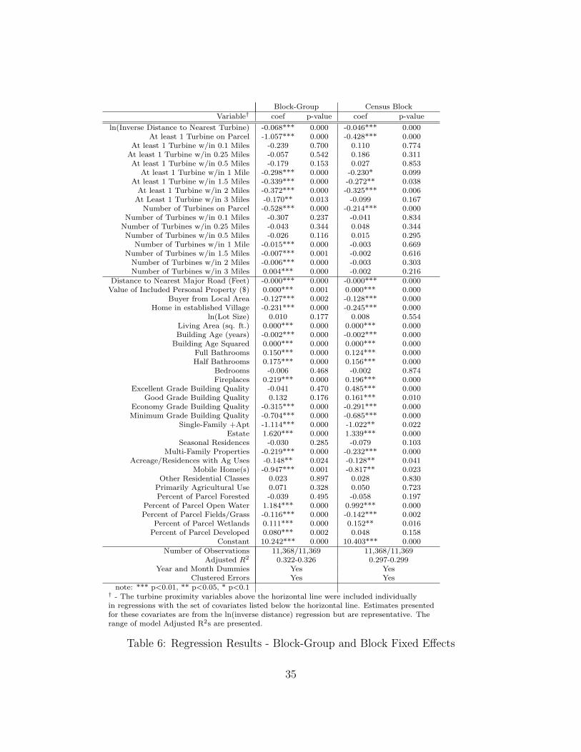
endogeneity bias because of the selection effects discussed above. In Table 6, we

display results of estimating Equation 1 including one wind variable at a time

with each of the other covariates.17 The rationale for this is that, except for the

distance variable, these measures are not exclusive of one another, and are thus

highly collinear. All of the results presented here assume that turbines exist

at the date the Final Environmental Impact Statement (EIS) is issued. This

accounts for the fact that local residents and most other participants in real

estate markets will be aware of at least the approximate location of turbines

before they are actually constructed. In fact, most of the turbine locations

19

would be known, if not publically, well before this since developers typically

negotiate with individual landowners before moving forward with regulatory

approvals. Our results are quite robust to adjusting the date of ‘existence’

forwards to the date of the draft EIS. If we adjust this date backwards to the

date of the permit being issued the results are qualitatively similar, but we lose

significance - likely because we then have even fewer post-turbine transactions

in the ‘treatment’ group.

First, notice that the covariate results are largely as would be predicted.

Homeowners in this region prefer larger homes, more bathrooms and fireplaces,

and to be close to major roads. The road result may be counter-intuitive, but

remember the rural character of our study area; distance to a major road is a

measure of the relative isolation of a parcel. Homeowners also take into account

the value of included property, and appear to prefer to be outside of established

villages. This may be a tax story as those homeowners in outlying areas

face considerably lower property taxes. However, homes outside of villages

generally have larger lots. Lot size is, unusually, not a significant factor. This

may be because of the large size of most parcels in our sample, but also may

be related to the inclusion of the village identifier.18 Local buyers pay about

9% less than others.19 Residents appear to not value additional bedrooms,

but since we are controlling for house size, this result is likely because, ceteris

paribus, more bedrooms means smaller bedrooms. Not surprisingly, parcels

with more dedicated agricultural land are priced lower, controlling for acreage,

and homes with open water or wetlands are more valuable. These measures

are partially proxying for a home being waterfront. The presence of multiple

20

families, including apartments, or mobile homes on a parcel also reduce the

price, while ‘estates’ receive a premium.20 Strangely, homes classified as having

‘excellent’ construction quality appear to sell for less than those with average

quality in the block-group model while selling for more in the census block

model. The negative, insignificant, result is likely to due to the small number

of homes with this classification and omitted variables bias that is corrected for

in the census block model. Meanwhile, minimum and economy quality homes

sell at substantial discounts of about 50.5% and 27% respectively relative to

average quality homes. Finally, age has a negative but diminishing impact as

older homes, all else equal, will sell for less.

The wind results are also broadly consistent with intuition. At the block-

group level, the existence of turbines between up to 1 and 3 miles away neg-

atively impacts property values by between 15.6% and 31%, while having at

least one turbine on the parcel reduces prices by 65%. The significance of this

last result is surprising given that only 3 parcels in our sample contain turbines

at the time of sale and thus may be spurious. Effects for turbines at other

distances are also negative though insignificant, and this is likely, and in part,

because of a lack of variation in these variables; only 39 of the observations

in our sample have turbines within 0.5 miles at the time of sale (about 0.3%).

We also find that the marginal turbine has a negative effect at all ranges and is

significant in the same ranges as above. At the block level we see many of the

same effects, with turbines in the 0.1 mile range also having significant effects.

At both scales, the ln(inverse distance) measure is significant and negative.

We will discuss the interpretation of this coefficient in Section 5.

21

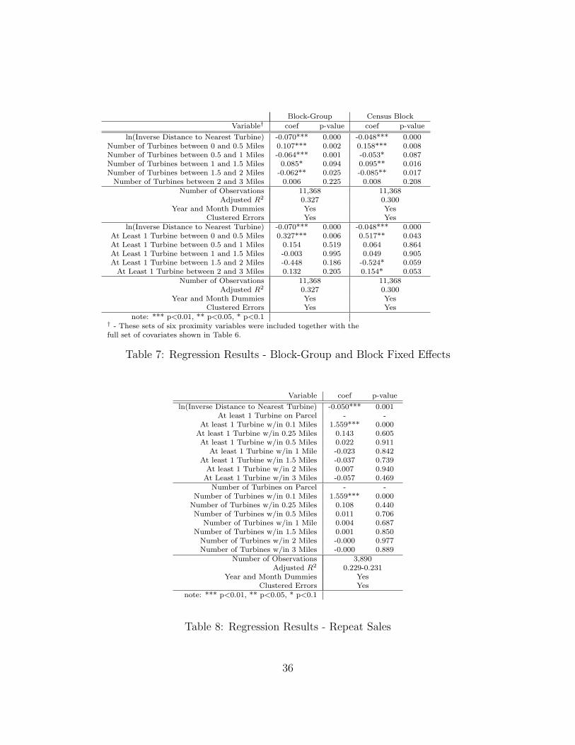
Table 7 contains results from using two additional sets of variables to rep-

resent the effects of wind turbines. These are dummy variables and count

variables representing the existence of turbines within concentric rings around

each parcel.21 The ln(inverse distance) measure is also included as a covari-

ate, and, as above, it is negative and significant. These measures show less

consistent results than those above. At very small distances there appears to

be a positive effect with the sign switching between positive and negative at

larger distances. These results are robust to excluding the ln(inverse distance)

variable. One reason for the inconsistent and generally insignificant results

for these estimates is that even though these measures are not dependent on

one another, there is still a high degree of collinearity between the number of

turbines within each of the ranges.

All of the results in Table 6 and Table 7, however, are subject to endogene-

ity bias. If it is true that lower value parcels are more likely to contain or be

near wind turbines due to selection effects, than these estimates would over-

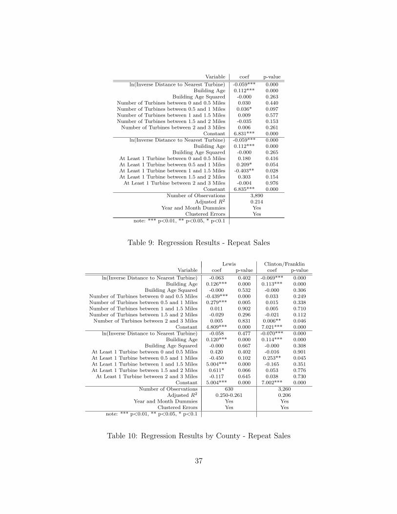
state the negative impact of turbine proximity. Tables 8 and 9 present results

from the estimation of Equation 2 that control for these selection effects using

parcel-level fixed effects. Specifically, Table 8 presents results from using each

turbine measure individually in regressions with only year and month dummies

and the age of the home and Table 9 presents results from using the distance

measure with the concentric circle turbine dummies and count variables. Here

we see a consistent negative impact from proximity to the nearest turbine, and

little other significance. We do find a significant positive impact from having

turbines within 0.1 miles when proximity measures are included individually,

22

and weakly significant positive impacts for turbines between 0.5 and 1 mile

away as well as negative impacts for turbines between 1 and 1.5 miles away

in the concentric circle model. These results are plausible if homes very close

to existing turbines expect that future wind development may be possible on

their parcels, which would necessitate easement payments.

The coefficient on age is now positive and significant. This sign reversal

might be explained by the fact that, in the repeat-sales framework, this variable

represents the change in age, or the number of years between sales for a parcel.

We are controlling for the dynamics of the real estate market through year and

month dummy variables, but this may be acting as an additional control for

general appreciation over the sample period.

Throughout all of these regressions, however, the ln(inverse distance) mea-

sure is strongly significant and negative, which indicates that wind turbines

are negatively impacting property values in a way that is declining over the

distance from the turbines. Notice that the effects are somewhat larger in the

block-group model than in the census block or repeat sales models. This is

suggestive of endogeneity bias in the block-group model.

We would expect there to be systematic differences in the effects of wind

turbines across the counties in our sample. In particular, the turbines in Lewis

County were installed in 2004-2005 and those in Clinton and Franklin County

were only installed in 2008-2009. So, homeowners in Lewis County have more

experience with the turbines and, in addition, we observe more post-turbine

transactions in Lewis County with which to identify impacts. Table 10 reports

repeat sales results by area - Lewis County vs. Clinton/Franklin Counties. We

23

combine Clinton and Franklin Counties since the turbines in these counties

were installed at very close to the same time and the wind farms are nearly

adjacent to one another. We see that proximity effects are still negative, but

not significant in Lewis County, which is somewhat surprising, but may result

from the small number of observations, or from the fact that familiarity with

the turbines has diminished their impact. Meanwhile, proximity effects are

negative and strongly significant in Clinton/Franklin Counties. In both areas

there continue to be unexplained significant impacts from turbines within some

concentric circles.

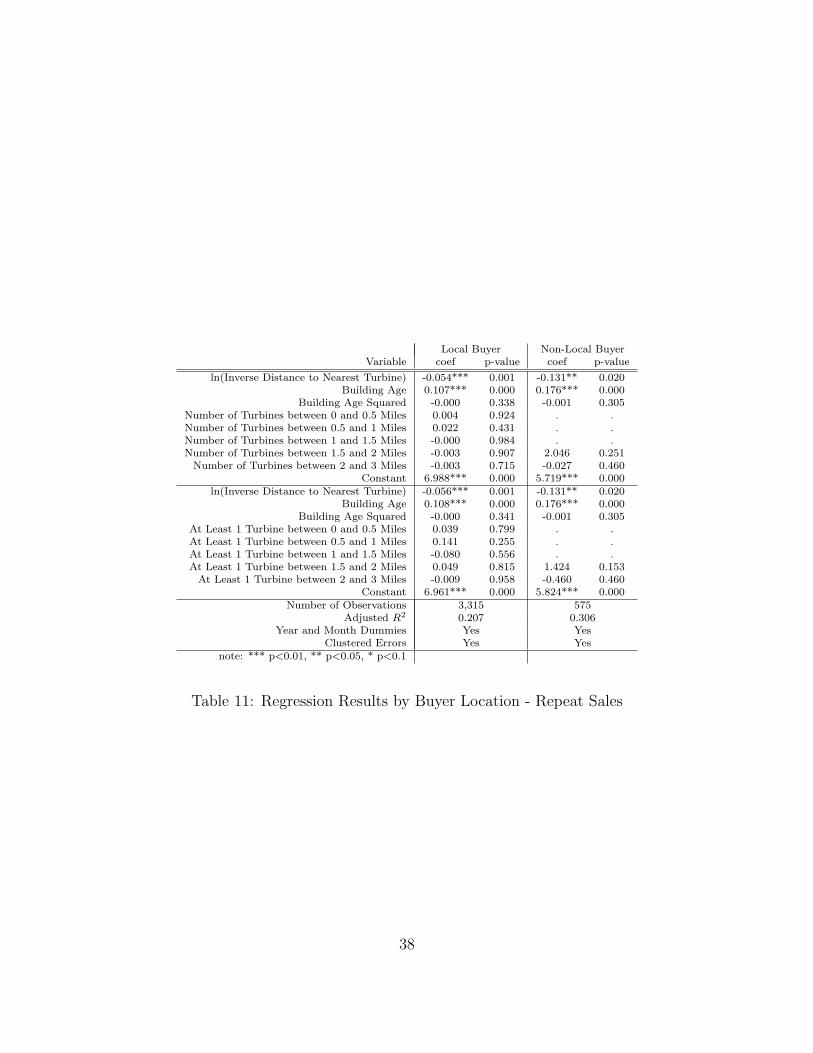
Another interesting way to segment the data is along the dimension of

whether or not the buyers in a transaction are local residents (from the five

counties that make up the North Country). The idea is that local buyers

might be more aware of the effects of turbines, particularly after the fact, and

also more likely to know about turbine locations and potential locations. In

Table 11 we see that the proximity effect is more than halved for local buyers

vs. non-local buyers.22 This suggests that non-local buyers are more wary of

turbines and their effects than local residents which may also be a function of

familiarity.

5 Discussion and Conclusions

The results in this study appear to indicate that proximity to wind turbines

does have a negative and significant impact on property values. Importantly,

the best and most consistent measure of these effects appears to be the simple,

24

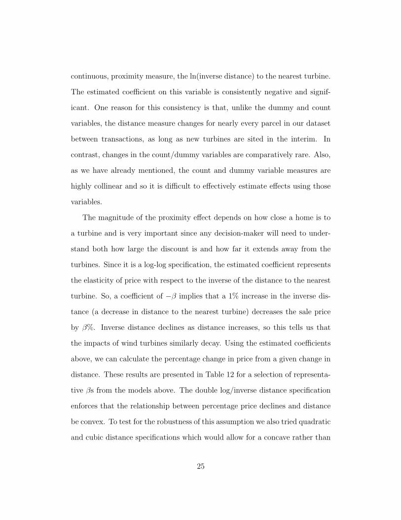
continuous, proximity measure, the ln(inverse distance) to the nearest turbine.

The estimated coefficient on this variable is consistently negative and signif-

icant. One reason for this consistency is that, unlike the dummy and count

variables, the distance measure changes for nearly every parcel in our dataset

between transactions, as long as new turbines are sited in the interim. In

contrast, changes in the count/dummy variables are comparatively rare. Also,

as we have already mentioned, the count and dummy variable measures are

highly collinear and so it is difficult to effectively estimate effects using those

variables.

The magnitude of the proximity effect depends on how close a home is to

a turbine and is very important since any decision-maker will need to under-

stand both how large the discount is and how far it extends away from the

turbines. Since it is a log-log specification, the estimated coefficient represents

the elasticity of price with respect to the inverse of the distance to the nearest

turbine. So, a coefficient of −β implies that a 1% increase in the inverse dis-

tance (a decrease in distance to the nearest turbine) decreases the sale price

by β%. Inverse distance declines as distance increases, so this tells us that

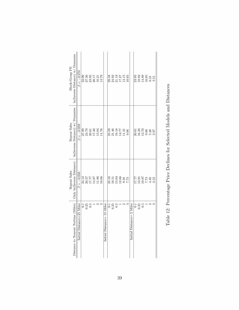
the impacts of wind turbines similarly decay. Using the estimated coefficients

above, we can calculate the percentage change in price from a given change in

distance. These results are presented in Table 12 for a selection of representa-

tive βs from the models above. The double log/inverse distance specification

enforces that the relationship between percentage price declines and distance

be convex. To test for the robustness of this assumption we also tried quadratic

and cubic distance specifications which would allow for a concave rather than

25

convex relationship. The quadratic specification confirmed the convex shape

of the relationship since the linear term was positive and significant and the

quadratic term was negative and significant. The quadratic and cubic terms

in the cubic specification were not significant.23

From the repeat sales model we see that the construction of turbines such

that for a given home the nearest turbine is now only 0.5 miles away results

in a 10.87%-17.77% decline in sales price depending on the initial distance to

the nearest turbine and the particular specification. For the average property

in our sample that sells for $106,864, this implies a loss in value of between

$11,616 and $18,990. At a distance of 1 mile (about 20% of our sample), we

see declines in value of between 7.73% and 14.87% resulting in losses for the

average home of between $8,261 and $15,891. Failing to properly control for

selection effects, as in the block-group fixed effects analysis, results in price

declines that are about 35% higher than those estimated from the repeat sales

model.

From a policy perspective, these results indicate that there remains a need

to compensate local homeowners/communities for allowing wind development

within their borders. Existing PILOT programs and compensation to indi-

vidual landowners are implicitly accounted for in this analysis since we would

expect these payments to be capitalized into sales prices, and still we find neg-

ative impacts. This suggests that landowners, particularly those who do not

have turbines on their properties and are thus not receiving direct payments

from wind developers, are being harmed and have an economic case to make

for more compensation. That is, while the ‘markets’ for easements and PILOT

26

programs may be properly accounting for harm to those who allow parcels on

their property, it appears not to be accounting for harm to others nearby. This

is a clear case of an uncorrected externality. If, in the future, developers are

forced to account for this externality through increased payments this would

obviously increase the cost to developers and make it that much more difficult

to economically justify wind projects.

This study does not say anything about the societal benefits from wind

power and should not be interpreted as saying that wind development should

be stopped. If, in fact, wind power is being used to displace fossil-based elec-

tricity generation it may still be that the environmental benefits of such a

trade exceed the costs. However, in comparing those environmental benefits,

we must include not only costs to developers (which include easement pay-

ments and PILOT programs), but also these external costs to property owners

local to new wind facilities. Property values are an important component

of any cost-benefit analysis and should be accounted for as new projects are

proposed and go through the approval process.

Finally, this paper breaks with the prior literature in finding any statisti-

cally significant property-value impacts from wind facilities. We believe that

this stems from our empirical approach which controls for omitted variables

and endogeneity biases. Future studies which expand this sort of analysis to

wind and other renewable power facilities in other regions are imperative to

understanding the big picture of what will happen as these technologies grow

in prominence.

27

References

[1] Spencer Banzhaf, Dallas Burtraw, David Evans, and Alan Krupnick. Val-

uation of natural resource improvements in the adirondacks. Land Eco-

nomics, 82(3):1–43, 2006.

[2] Marianne Bertrand, Esther Duflo, and Sendhil Mullainathan. How much

should we trust differences-in-differences estimates? Quarterly Journal of

Economics, 119:249–275, February 2004.

[3] W. David Colby, Robert Dobie, Geoff Leventhall, David M. Libscomb,

Robert J. McCunney, Michael T. Seilo, and Bo Sondergaard. Wind tur-

bine sound and health effects: An expert panel review. American Wind

Energy Association, 2009.

[4] Katherine Daniels. Wind energy: Model ordinance options. NYSERDA,

October 2005.

[5] Michael Greenstone and Ted Gayer. Quasi-experiments and experimen-

tal approaches to environmental economics. Journal of Environmental

Economics and Management, 57:21–44, 2009.

[6] Peter A. Groothuis, Jana D. Groothuis, and John C. Whitehead. Green

vs. green: Measuring the compensation required to site electrical genera-

tion windmills in a viewshed. Energy Policy, 36:1545–1550, 2008.

[7] Robert Halvorsen and Raymond Palmquist. The interpretation of dummy

variables in semilogarithmic equations. American Economic Review,

70(3):474–475, June 1980.

28

[8] Martin D. Heintzelman. Measuring the property value effects of land-use

and preservation referenda. Land Economics, 86(1), February 2010a.

[9] Martin D. Heintzelman. The value of land use patterns and preservation

policies. The B.E. Journal of Economics Analysis and Policy (Topics),

10(1), 2010b. Article 39.

[10] Ben Hoen. Impacts of windmill visibility on property values in madison

county, new york. Master’s thesis, Bard Center for Environmental Policy,

Bard College, Annandale-on-Hudson, NY, April 2006.

[11] Ben Hoen, Ryan Wiser, Peter Cappers, Mark Thayer, and Gautam Sethi.

The impact of wind power projects on residential property values in the

united states: A multi-site hedonic analysis. Technical Report LBNL-

2829E, Ernest Orlando Lawrence Berkeley National Laboratory, Envi-

ronmental Energy Technologies Division, December 2009.

[12] Andrew D. Krueger, George R. Parsons, and Jeremy Firestone. Valu-

ing the visual disamenity of offshore wind power projects at varying dis-

tances from the shore: An application on the delaware shoreline. Land

Economics, 87(2):268–283, May 2011.

[13] Chris Parmeter and Jaren C. Pope. Quasi-experiments and hedonic prop-

erty value methods. In John A. List and Michael K. Price, editors, Hand-

book on Experimental Economics and the Environment. Edward Elgar

Publishing, 2011.

29

[14] Sally Sims and Peter Dent. Property stigma: Wind farms are just the

latest fashion. Journal of Property Investment and Finance, 25(6):626–

651, 2007.

[15] Sally Sims, Peter Dent, and G. Reza Oskrochi. Modelling the impact of

wind farms on house prices in the uk. International Journal of Strategic

Property Management, 12:251–269, 2008.

[16] George Sterzinger, Frederic Beck, and Damian Kostiuk. The effect of

wind development on local property values. Analytical report, Renewable

Energy Policy Project, May 2003.

[17] Jeffrey M. Wooldridge. Econometric Analysis of Cross Section and Panel

Data. The MIT Press, 2002.

30

Tables and Figures

31

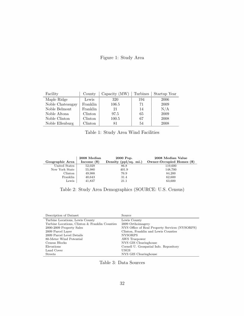
Figure 1: Study Area

Facility County Capacity (MW) Turbines Startup YearMaple Ridge Lewis 320 194 2006Noble Chateaugay Franklin 106.5 71 2009Noble Belmont Franklin 21 14 N/ANoble Altona Clinton 97.5 65 2009Noble Clinton Clinton 100.5 67 2008Noble Ellenburg Clinton 81 54 2008

Table 1: Study Area Wind Facilities

2008 Median 2000 Pop. 2008 Median ValueGeographic Area Income ($) Density (ppl/sq. mi.) Owner-Occupied Homes ($)

United States 52,029 86.8 119,600New York State 55,980 401.9 148,700

Clinton 49,988 76.9 84,200Franklin 40,643 31.4 62,600

Lewis 41,837 21.1 63,600

Table 2: Study Area Demographics (SOURCE: U.S. Census)

Description of Dataset Source

Turbine Locations, Lewis County Lewis CountyTurbine Locations, Clinton & Franklin Counties 2009 Orthoimagery2000-2009 Property Sales NYS Office of Real Property Services (NYSORPS)2009 Parcel Layer Clinton, Franklin and Lewis Counties2009 Parcel Level Details NYSORPS80-Meter Wind Potential AWS TruepowerCensus Blocks NYS GIS ClearinghouseElevations Cornell U. Geospatial Info. RepositoryLand Cover USGSStreets NYS GIS Clearinghouse

Table 3: Data Sources

32

Clinton Franklin LewisVariable Mean Std. Dev Mean Std. Dev Mean Std. Dev

Sale Price ($) $122,645 $83,603 $120,466 $354,556 $81,740 $63,207Building Age (years) 37 41 49 109 50 42Living Area (sq. ft.) 1,609 611 1,447 643 1,538 690

Lot Size (acres) 5.9 39.3 6.8 25.6 9.0 27.2Distance to Nearest Major Road (Feet) 1,549 2,493 1,861 3,189 6,094 6,628

Value of Included Personal Property ($) $63 $965 $324 $6,995 $204 $2,678Buyer from Local Area 0.913 0.282 0.790 0.407 0.684 0.465

Home in established Village 0.049 0.215 0.395 0.489 0.261 0.439Full Bathrooms 1.615 0.647 1.312 0.618 1.287 0.630Half Bathrooms 0.332 0.495 0.226 0.441 0.229 0.431

Bedrooms 3.134 0.936 2.829 1.051 2.929 1.140Fireplaces 0.306 0.544 0.245 0.484 0.167 0.416

Excellent Grade Building Quality 0 0 0 0 0.0005 0.023Good Grade Building Quality 0.031 0.173 0.019 0.137 0.013 0.112

Average Grade Building Quality 0.833 0.373 0.584 0.493 0.639 0.480Economy Grade Building Quality 0.136 0.342 0.381 0.486 0.317 0.465Minimum Grade Building Quality 0.001 0.028 0.016 0.127 0.031 0.174

Single-Family 0.859 0.348 0.755 0.430 0.677 0.468Single-Family +Apt 0.001 0.025 0 0 0 0

Estate 0.0002 0.013 0.003 0.058 0 0Seasonal Residences 0.032 0.175 0.111 0.314 0.181 0.385

Multi-Family Properties 0.054 0.226 0.046 0.209 0.043 0.203Acreage/Residences with Ag Uses 0.043 0.202 0.054 0.226 0.054 0.225

Mobile Home(s) 0.0003 0.018 0.002 0.039 0.006 0.075Other Residential Classes 0.007 0.081 0.012 0.107 0.011 0.106

Primarily Agricultural Use 0.005 0.071 0.018 0.135 0.029 0.168Percent of Parcel Forested 0.202 0.324 0.269 0.353 0.319 0.371

Percent of Parcel Open Water 0.011 0.077 0.031 0.127 0.024 0.123Percent of Parcel Fields/Grass 0.160 0.293 0.139 0.277 0.292 0.356

Percent of Parcel Wetlands 0.041 0.147 0.068 0.172 0.067 0.170Percent of Parcel Developed 0.444 0.448 0.226 0.369 0.134 0.293

Percent of Parcel Open 0.141 0.256 0.268 0.344 0.164 0.290Observations 6,159 3,255 1,955

Table 4: Summary Statistics by County

33

Clinto

nF

ran

klin

Lew

isV

ari

ab

leM

ean

Std

.D

ev.

Max.

Mea

nS

td.

Dev

.M

ax.

Mea

nS

td.

Dev

.M

ax.

Dis

tan

ceto

Nea

rest

Tu

rbin

e(m

iles

)11.2

4.2

28.9

24.1

15.0

53.5

9.4

6.4

26.7

Inver

seD

ista

nce

toN

eare

stT

urb

ine

0.1

0.4

18.0

0.2

1.5

81.1

0.2

0.8

24.4

Nu

mb

erof

Tu

rbin

eson

Parc

el0.0

01

0.0

46

30.0

00

0.0

18

10.0

01

0.0

23

1N

um

ber

of

Tu

rbin

esw

/in

0.1

Miles

0.0

02

0.0

89

60.0

02

0.0

66

30.0

03

0.0

71

2N

um

ber

of

Tu

rbin

esw

/in

0.2

5M

iles

0.0

07

0.2

12

13

0.0

05

0.1

37

60.0

27

0.3

47

10

Nu

mb

erof

Tu

rbin

esw

/in

0.5

Miles

0.0

23

0.4

57

18

0.0

37

0.5

05

19

0.0

54

0.5

84

12

Nu

mb

erof

Tu

rbin

esw

/in

1M

ile

0.0

92

1.4

37

42

0.2

19

1.5

78

39

0.1

94

1.7

74

26

Nu

mb

erof

Tu

rbin

esw

/in

1.5

Miles

0.2

06

2.8

03

65

0.5

03

3.2

36

70

0.4

65

3.5

94

53

Nu

mb

erof

Tu

rbin

esw

/in

2M

iles

0.3

57

4.4

23

103

0.8

79

5.3

55

92

0.8

53

5.8

87

82

Nu

mb

erof

Tu

rbin

esw

/in

3M

iles

0.7

21

7.6

65

162

2.0

84

10.7

73

152

2.2

65

11.4

39

114

At

least

1T

urb

ine

on

Parc

el0.0

003

0.0

18

10.0

003

0.0

18

10.0

01

0.0

23

1A

tle

ast

1T

urb

ine

w/in

0.1

Miles

0.0

01

0.0

28

10.0

01

0.0

30

10.0

02

0.0

45

1A

tle

ast

1T

urb

ine

w/in

0.2

5M

iles

0.0

02

0.0

48

10.0

02

0.0

46

10.0

09

0.0

96

1A

tle

ast

1T

urb

ine

w/in

0.5

Miles

0.0

04

0.0

62

10.0

13

0.1

13

10.0

12

0.1

10

1A

tle

ast

1T

urb

ine

w/in

1M

ile

0.0

06

0.0

79

10.0

32

0.1

75

10.0

20

0.1

42

1A

tle

ast

1T

urb

ine

w/in

1.5

Miles

0.0

08

0.0

92

10.0

36

0.1

87

10.0

27

0.1

62

1A

tle

ast

1T

urb

ine

w/in

2M

iles

0.0

12

0.1

07

10.0

41

0.1

97

10.0

33

0.1

79

1A

tL

east

1T

urb

ine

w/in

3M

iles

0.0

19

0.1

38

10.0

57

0.2

32

10.1

04

0.3

05

1N

um

ber

of

Tu

rbin

esb

etw

een

0an

d0.5

Miles

0.0

22

0.4

27

16

0.0

37

0.4

94

18

0.0

53

0.5

73

11

Nu

mb

erof

Tu

rbin

esb

etw

een

0.5

an

d1

Miles

0.0

69

1.0

28

25

0.1

82

1.1

83

20

0.1

41

1.2

34

17

Nu

mb

erof

Tu

rbin

esb

etw

een

1an

d1.5

Miles

0.1

14

1.4

44

31

0.2

84

1.7

66

31

0.2

71

1.9

39

27

Nu

mb

erof

Tu

rbin

esb

etw

een

1.5

an

d2

Miles

0.1

52

1.7

37

42

0.3

77

2.2

47

34

0.3

88

2.4

99

35

Nu

mb

erof

Tu

rbin

esb

etw

een

2an

d3

Miles

0.3

64

3.6

33

87

1.2

05

5.8

66

64

1.4

13

6.1

31

54

At

Lea

st1

Tu

rbin

eb

etw

een

0an

d0.5

Miles

0.0

04

0.0

62

10.0

13

0.1

13

10.0

12

0.1

10

1A

tL

east

1T

urb

ine

bet

wee

n0.5

an

d1

Miles

0.0

06

0.0

79

10.0

32

0.1

75

10.0

20

0.1

42

1A

tL

east

1T

urb

ine

bet

wee

n1

an

d1.5

Miles

0.0

08

0.0

92

10.0

36

0.1

87

10.0

27

0.1

62

1A

tL

east

1T

urb

ine

bet

wee

n1.5

an

d2

Miles

0.0

12

0.1

07

10.0

41

0.1

97

10.0

33

0.1

79

1A

tL

east

1T

urb

ine

bet

wee

n2

an

d3

Miles

0.0

19

0.1

38

10.0

57

0.2

32

10.1

04

0.3

05

1

Tab

le5:

Sum

mar

ySta

tist

ics

for

Win

dT

urb

ine

Var

iable

sin

2009

34

Block-Group Census Block

Variable† coef p-value coef p-value

ln(Inverse Distance to Nearest Turbine) -0.068*** 0.000 -0.046*** 0.000At least 1 Turbine on Parcel -1.057*** 0.000 -0.428*** 0.000

At least 1 Turbine w/in 0.1 Miles -0.239 0.700 0.110 0.774At least 1 Turbine w/in 0.25 Miles -0.057 0.542 0.186 0.311At least 1 Turbine w/in 0.5 Miles -0.179 0.153 0.027 0.853

At least 1 Turbine w/in 1 Mile -0.298*** 0.000 -0.230* 0.099At least 1 Turbine w/in 1.5 Miles -0.339*** 0.000 -0.272** 0.038

At least 1 Turbine w/in 2 Miles -0.372*** 0.000 -0.325*** 0.006At Least 1 Turbine w/in 3 Miles -0.170** 0.013 -0.099 0.167

Number of Turbines on Parcel -0.528*** 0.000 -0.214*** 0.000Number of Turbines w/in 0.1 Miles -0.307 0.237 -0.041 0.834

Number of Turbines w/in 0.25 Miles -0.043 0.344 0.048 0.344Number of Turbines w/in 0.5 Miles -0.026 0.116 0.015 0.295

Number of Turbines w/in 1 Mile -0.015*** 0.000 -0.003 0.669Number of Turbines w/in 1.5 Miles -0.007*** 0.001 -0.002 0.616

Number of Turbines w/in 2 Miles -0.006*** 0.000 -0.003 0.303Number of Turbines w/in 3 Miles 0.004*** 0.000 -0.002 0.216

Distance to Nearest Major Road (Feet) -0.000*** 0.000 -0.000*** 0.000Value of Included Personal Property ($) 0.000*** 0.001 0.000*** 0.000

Buyer from Local Area -0.127*** 0.002 -0.128*** 0.000Home in established Village -0.231*** 0.000 -0.245*** 0.000

ln(Lot Size) 0.010 0.177 0.008 0.554Living Area (sq. ft.) 0.000*** 0.000 0.000*** 0.000Building Age (years) -0.002*** 0.000 -0.002*** 0.000

Building Age Squared 0.000*** 0.000 0.000*** 0.000Full Bathrooms 0.150*** 0.000 0.124*** 0.000Half Bathrooms 0.175*** 0.000 0.156*** 0.000

Bedrooms -0.006 0.468 -0.002 0.874Fireplaces 0.219*** 0.000 0.196*** 0.000

Excellent Grade Building Quality -0.041 0.470 0.485*** 0.000Good Grade Building Quality 0.132 0.176 0.161*** 0.010

Economy Grade Building Quality -0.315*** 0.000 -0.291*** 0.000Minimum Grade Building Quality -0.704*** 0.000 -0.685*** 0.000

Single-Family +Apt -1.114*** 0.000 -1.022** 0.022Estate 1.620*** 0.000 1.339*** 0.000

Seasonal Residences -0.030 0.285 -0.079 0.103Multi-Family Properties -0.219*** 0.000 -0.232*** 0.000

Acreage/Residences with Ag Uses -0.148** 0.024 -0.128** 0.041Mobile Home(s) -0.947*** 0.001 -0.817** 0.023

Other Residential Classes 0.023 0.897 0.028 0.830Primarily Agricultural Use 0.071 0.328 0.050 0.723Percent of Parcel Forested -0.039 0.495 -0.058 0.197

Percent of Parcel Open Water 1.184*** 0.000 0.992*** 0.000Percent of Parcel Fields/Grass -0.116*** 0.000 -0.142*** 0.002

Percent of Parcel Wetlands 0.111*** 0.000 0.152** 0.016Percent of Parcel Developed 0.080*** 0.002 0.048 0.158

Constant 10.242*** 0.000 10.403*** 0.000Number of Observations 11,368/11,369 11,368/11,369

Adjusted R2 0.322-0.326 0.297-0.299Year and Month Dummies Yes Yes

Clustered Errors Yes Yesnote: *** p<0.01, ** p<0.05, * p<0.1

† - The turbine proximity variables above the horizontal line were included individuallyin regressions with the set of covariates listed below the horizontal line. Estimates presentedfor these covariates are from the ln(inverse distance) regression but are representative. Therange of model Adjusted R2s are presented.

Table 6: Regression Results - Block-Group and Block Fixed Effects

35

Block-Group Census Block

Variable† coef p-value coef p-value

ln(Inverse Distance to Nearest Turbine) -0.070*** 0.000 -0.048*** 0.000Number of Turbines between 0 and 0.5 Miles 0.107*** 0.002 0.158*** 0.008Number of Turbines between 0.5 and 1 Miles -0.064*** 0.001 -0.053* 0.087Number of Turbines between 1 and 1.5 Miles 0.085* 0.094 0.095** 0.016Number of Turbines between 1.5 and 2 Miles -0.062** 0.025 -0.085** 0.017

Number of Turbines between 2 and 3 Miles 0.006 0.225 0.008 0.208Number of Observations 11,368 11,368

Adjusted R2 0.327 0.300Year and Month Dummies Yes Yes

Clustered Errors Yes Yesln(Inverse Distance to Nearest Turbine) -0.070*** 0.000 -0.048*** 0.000

At Least 1 Turbine between 0 and 0.5 Miles 0.327*** 0.006 0.517** 0.043At Least 1 Turbine between 0.5 and 1 Miles 0.154 0.519 0.064 0.864At Least 1 Turbine between 1 and 1.5 Miles -0.003 0.995 0.049 0.905At Least 1 Turbine between 1.5 and 2 Miles -0.448 0.186 -0.524* 0.059

At Least 1 Turbine between 2 and 3 Miles 0.132 0.205 0.154* 0.053Number of Observations 11,368 11,368

Adjusted R2 0.327 0.300Year and Month Dummies Yes Yes

Clustered Errors Yes Yesnote: *** p<0.01, ** p<0.05, * p<0.1

† - These sets of six proximity variables were included together with thefull set of covariates shown in Table 6.

Table 7: Regression Results - Block-Group and Block Fixed Effects

Variable coef p-value

ln(Inverse Distance to Nearest Turbine) -0.050*** 0.001At least 1 Turbine on Parcel - -

At least 1 Turbine w/in 0.1 Miles 1.559*** 0.000At least 1 Turbine w/in 0.25 Miles 0.143 0.605At least 1 Turbine w/in 0.5 Miles 0.022 0.911

At least 1 Turbine w/in 1 Mile -0.023 0.842At least 1 Turbine w/in 1.5 Miles -0.037 0.739

At least 1 Turbine w/in 2 Miles 0.007 0.940At Least 1 Turbine w/in 3 Miles -0.057 0.469

Number of Turbines on Parcel - -Number of Turbines w/in 0.1 Miles 1.559*** 0.000

Number of Turbines w/in 0.25 Miles 0.108 0.440Number of Turbines w/in 0.5 Miles 0.011 0.706

Number of Turbines w/in 1 Mile 0.004 0.687Number of Turbines w/in 1.5 Miles 0.001 0.850

Number of Turbines w/in 2 Miles -0.000 0.977Number of Turbines w/in 3 Miles -0.000 0.889

Number of Observations 3,890Adjusted R2 0.229-0.231

Year and Month Dummies YesClustered Errors Yes

note: *** p<0.01, ** p<0.05, * p<0.1

Table 8: Regression Results - Repeat Sales

36

Variable coef p-value

ln(Inverse Distance to Nearest Turbine) -0.059*** 0.000Building Age 0.112*** 0.000

Building Age Squared -0.000 0.263Number of Turbines between 0 and 0.5 Miles 0.030 0.440Number of Turbines between 0.5 and 1 Miles 0.036* 0.097Number of Turbines between 1 and 1.5 Miles 0.009 0.577Number of Turbines between 1.5 and 2 Miles -0.035 0.153

Number of Turbines between 2 and 3 Miles 0.006 0.261Constant 6.831*** 0.000

ln(Inverse Distance to Nearest Turbine) -0.059*** 0.000Building Age 0.112*** 0.000

Building Age Squared -0.000 0.265At Least 1 Turbine between 0 and 0.5 Miles 0.180 0.416At Least 1 Turbine between 0.5 and 1 Miles 0.209* 0.054At Least 1 Turbine between 1 and 1.5 Miles -0.403** 0.028At Least 1 Turbine between 1.5 and 2 Miles 0.303 0.154

At Least 1 Turbine between 2 and 3 Miles -0.004 0.976Constant 6.835*** 0.000

Number of Observations 3,890Adjusted R2 0.214

Year and Month Dummies YesClustered Errors Yes

note: *** p<0.01, ** p<0.05, * p<0.1

Table 9: Regression Results - Repeat Sales

Lewis Clinton/FranklinVariable coef p-value coef p-value

ln(Inverse Distance to Nearest Turbine) -0.063 0.402 -0.069*** 0.000Building Age 0.126*** 0.000 0.113*** 0.000

Building Age Squared -0.000 0.532 -0.000 0.306Number of Turbines between 0 and 0.5 Miles -0.439*** 0.000 0.033 0.249Number of Turbines between 0.5 and 1 Miles 0.279*** 0.005 0.015 0.338Number of Turbines between 1 and 1.5 Miles 0.011 0.902 0.005 0.710Number of Turbines between 1.5 and 2 Miles -0.029 0.296 -0.021 0.112

Number of Turbines between 2 and 3 Miles 0.005 0.831 0.006** 0.046Constant 4.809*** 0.000 7.021*** 0.000

ln(Inverse Distance to Nearest Turbine) -0.058 0.477 -0.070*** 0.000Building Age 0.120*** 0.000 0.114*** 0.000

Building Age Squared -0.000 0.667 -0.000 0.308At Least 1 Turbine between 0 and 0.5 Miles 0.420 0.402 -0.016 0.901At Least 1 Turbine between 0.5 and 1 Miles -0.450 0.102 0.253** 0.045At Least 1 Turbine between 1 and 1.5 Miles 5.004*** 0.000 -0.165 0.351At Least 1 Turbine between 1.5 and 2 Miles 0.611* 0.066 0.053 0.776

At Least 1 Turbine between 2 and 3 Miles -0.117 0.645 0.038 0.730Constant 5.004*** 0.000 7.002*** 0.000

Number of Observations 630 3,260Adjusted R2 0.250-0.261 0.206

Year and Month Dummies Yes YesClustered Errors Yes Yes

note: *** p<0.01, ** p<0.05, * p<0.1

Table 10: Regression Results by County - Repeat Sales

37

Local Buyer Non-Local BuyerVariable coef p-value coef p-value

ln(Inverse Distance to Nearest Turbine) -0.054*** 0.001 -0.131** 0.020Building Age 0.107*** 0.000 0.176*** 0.000

Building Age Squared -0.000 0.338 -0.001 0.305Number of Turbines between 0 and 0.5 Miles 0.004 0.924 . .Number of Turbines between 0.5 and 1 Miles 0.022 0.431 . .Number of Turbines between 1 and 1.5 Miles -0.000 0.984 . .Number of Turbines between 1.5 and 2 Miles -0.003 0.907 2.046 0.251

Number of Turbines between 2 and 3 Miles -0.003 0.715 -0.027 0.460Constant 6.988*** 0.000 5.719*** 0.000

ln(Inverse Distance to Nearest Turbine) -0.056*** 0.001 -0.131** 0.020Building Age 0.108*** 0.000 0.176*** 0.000

Building Age Squared -0.000 0.341 -0.001 0.305At Least 1 Turbine between 0 and 0.5 Miles 0.039 0.799 . .At Least 1 Turbine between 0.5 and 1 Miles 0.141 0.255 . .At Least 1 Turbine between 1 and 1.5 Miles -0.080 0.556 . .At Least 1 Turbine between 1.5 and 2 Miles 0.049 0.815 1.424 0.153

At Least 1 Turbine between 2 and 3 Miles -0.009 0.958 -0.460 0.460Constant 6.961*** 0.000 5.824*** 0.000

Number of Observations 3,315 575Adjusted R2 0.207 0.306

Year and Month Dummies Yes YesClustered Errors Yes Yes

note: *** p<0.01, ** p<0.05, * p<0.1

Table 11: Regression Results by Buyer Location - Repeat Sales

38

Rep

eat

Sale

sR

epea

tS

ale

sB

lock

-Gro

up

FE

Dis

tan

ceto

Nea

rest

Tu

rbin

e(M

iles

)O

nly

ln(I

nver

seD

ista

nce

)ln

(Inver

seD

ista

nce

)w

/D

um

mie

sln

(Inver

seD

ista

nce

)w

/D

um

mie

s

Init

ial

Dis

tan

ce=

25

Mil

esβ

=−

0.0

50

β=−

0.0

59

β=−

0.0

70

0.1

24.1

227.8

032.0

60.2

520.5

723.7

927.5

60.5

17.7

720.6

123.9

51

14.8

717.3

020.1

72

11.8

613.8

416.2

13

10.0

611.7

613.7

9In

itia

lD

ista

nce

=15

Miles 0.1

22.1

625.5

929.5

80.2

518.5

121.4

624.9

20.5

15.6

418.1

821.1

91

12.6

614.7

717.2

72

9.5

811.2

113.1

53

7.7

39.0

610.6

5In

itia

lD

ista

nce

=5

Miles 0.1

17.7

720.6

123.9

50.2

513.9

116.2

018.9

20.5

10.8

712.7

014.8

91

7.7

39.0

610.6

52

4.4

85.2

66.2

13

2.5

22.9

73.5

1

Tab

le12

:P

erce

nta

geP

rice

Dec

lines

for

Sel

ecte

dM

odel

san

dD

ista

nce

s

39

Notes

1Data on the recent and future expected growth of wind energy are derived from the

Energy Information Administration of the U.S. Department of Energy ( http://www.eia.

doe.gov).

2These symptoms are described by Nina Pierpont in her book on the topic, Wind Turbine

Syndrome published in 2009.

3Renee Mickelburgh et al., “Huge protests by voters force the continent’s governments

to rethink so-called green energy”, Sunday Telegraph (London), April 4, 2004, p. 28.

4http://www.pachamber.org/www/products/publications/pdf/OSHA\%20Handbook\%20pgs287-291.

pdf

5See the DOI’s Cape Wind Fact sheet (http://www.doi.gov/news/doinews/upload/

04-28-10-Cape-Wind-Fact-Sheet-MMS-approved.pdf) for details on the regulatory pro-

cess surrounding the project.

6“WPEG sues Cape Vincent; Petition asks judge to nullify approval of impact state-

ment,” Watertown Daily Times, October 28, 2010.

7“Not on My Beach, Please,” The Economist, August 19, 2010.

8“Cape Vincent Wind Turbine Development Economic Impact - Final Report”, Submit-

ted by Wind Turbine Economic Impact Committee, Town of Cape Vincent, NY, October

7, 2010.

9Department of Energy (http://www.windpoweringamerica.gov/wind_installed_capacity.

asp).

10Department of Energy (http://www.windpoweringamerica.gov/wind_maps.asp).

11NYS Dept. of Environmental Conservation ( http://www.dec.ny.gov/docs/permits_

ej_operations_pdf/windstatuscty.pdf).

12The Final Environmental Impact Statement for the Noble Belmont project in Franklin

County was completed in conjunction with the Noble Chateaugay project. Construction

for the combined project consisting of 85 turbines was initiated in 2008. While 71 turbines

were brought online in 2009, site work for the additional 14 turbines was completed but the

40

turbines themselves were never installed. Since the turbine bases are visible from ortho-

imagery and the project environmental review was completed as a single project, these

locations have been included in our analysis.

13We measure the linear distance rather than road network distance since the effects are

not a matter of travel to or from the turbines, but instead simple proximity.

14In our particular study area, there are 92,960 total parcels, 1,997 census blocks, and

17 census block groups, which implies that, on average, there are 46.55 parcels per block,

5,468.24 parcels per block group. The average census block has an area of just under 2

square miles, and the average census block group, about 232 square miles.

15We also attempted an instrumental variables approach to this problem using two in-

struments - the wind potential of each parcel and the elevation of each parcel. The first was

strongly correlated with the location of turbines, but also correlated with property values

- parcels that are exposed to higher winds are less desirable. The second instrument was

not correlated with property values in our sample, but was not a strong predictor of the

location of turbines. For these reasons, we abandoned this approach.

16Spatial autocorrelation, when applied at the property level in a repeat sales analysis, is

similar to serial correlation in that the error term in one transaction is likely to be correlated

with the error term in a transaction of the same property at a different date.

17The covariate results presented here are from the first regression (that with just the

ln(inverse distance)), but are representative of results from the other regressions. Detailed

results are available from the authors.

18These two variables are negatively correlated in our sample. The correlation coefficient

is -0.2854.

19Percentage effects throughout are calculated following Halvorsen and Palmquist (1980)

who showed that the appropriate interpretation of dummy variable coefficients when using

a semi-log specification is g = ec − 1 where c is the estimated coefficient.

20Estates are defined according to NYSORPS as “A residential property of not less than

5 acres with a luxurious residence and auxiliary buildings.”

21Note that the full set of other covariates are included in these regressions. Results are

41

broadly consistent with those already presented, so they are not reported here.

22The distribution of local vs. non-local buyers differs somewhat between counties. Buyers

in Lewis County are less likely to be local with about 32% of Lewis County sales being non-

local as opposed to 21% in Clinton/Franklin Counties.

23We also tested log-linear inverse distance and log-linear distance specifications and the

results were consistent with those reported here. There was no evidence that these alterna-

tive specifications provided a better fit to the data.

42