1

Valuation of Reverse Mortgages

An Empirical Investigation using Portuguese Data

Ana Cristina Santos Gonçalves

Dissertation report presented as partial requirement for obtaining the Master’s degree in Statistics and Information Management - Specialization in Risk Analysis and Management

i

NOVA Information Management School

Instituto Superior de Estatística e Gestão de Informação

Universidade Nova de Lisboa

VALUATION OF REVERSE MORTGAGES:

AN EMPIRICAL INVESTIGATION USING PORTUGUESE DATA

by

Ana Cristina Santos Gonçalves

Dissertation report presented as partial requirement for obtaining the Master’s degree in Statistics and Information Management, with a specialization in Risk Analysis and Management

Advisor: Jorge Miguel Ventura Bravo

November 2017

ii

ACKNOWLEDGEMENTS

The author acknowledge the very important support of Professor Jorge Miguel Ventura Bravo and of

everyone, including family, friends and teachers, that somehow contributed to the completion of this

work.

iii

ABSTRACT

The increase of the average lifetime and the consequent population ageing is a growing reality in many countries, mainly due to the healthcares advancements and to the better living conditions in general. Portugal is not an exception and the need for long-term care services and their financing is raising. Reverse mortgages were originally conceived to assist retirees with limited income, to use their accumulated real wealth to cover daily living expenses and/or pay for health care. Considering the low-income level of most Portuguese retirees and the comparatively high levels of home ownership, the aim of this paper is to discuss the valuation of standard reverse mortgages contracts in Portugal using a stochastic approach for both biometric and financial risk factors. A vector autoregressive model is used to simulate the joint dynamics of economic variables like house price index, gross domestic product, consumer price index, mortgage rates and euro area yields. A stochastic mortality model (Poisson Lee-Carter age-period model) is used to project future mortality rates and to derive dynamic lifetables projections for the Portuguese population. All these results are used to calculate the reverse mortgage model and simulate results in different scenarios considering changes in relevant variables: initial borrower's age, initial house price, mortality rates, borrowing ratio, loan to value percentage and interest rate on the loan. The expected payoffs are compared and riskiness of the different scenarios is assessed using Value-at-Risk and Conditional Value-at-Risk.

KEYWORDS

Reverse Mortgage; Lifetime Mortgages; Equity Release; Lee-Carter Model; Termination Model; Vector Auto-Regressive Model; Risk-Based Capital

iv

RESUMO

O aumento da esperança média de vida e o consequente envelhecimento da população é uma realidade crescente em muitos países e deve-se maioritariamente aos avanços nos cuidados de saúde e às melhores condições de vida, em geral. Portugal não é uma excepção e a necessidade de serviços de cuidados de saúde continuados e do seu respetivo financiamento está a crescer. As Hipotecas Inversas foram originalmente concebidas para apoiar reformados com recursos financeiros limitados de forma a que pudessem usar o capital imobiliário para cobrir as despesas diárias e/ou pagar os cuidados de saúde. Considerando o baixo rendimento da maioria dos reformados portugueses e os comparativamente elevados níveis de detenção de habitação própria e permanente, este estudo visa analisar a avaliação de contractos padrão de Hipoteca Inversa em Portugal com uma abordagem estocástica para ambos os factores de riscos biométricos e financeiros. Um modelo de vector autoregressivo é usado para simular a dinâmica conjunta de variáveis económicas tais como o índice de preços da habitação, o produto interno bruto, o índice de preços no consumidor, as taxas de crédito à habitação e as taxas de rendibilidade da zona euro. Um modelo de mortalidade estocástico (modelo Poisson Lee-Carter age-period) é usado para projectar taxas de mortalidade futuras e para obter projecções de tábuas de mortalidade dinâmicas para a população portuguesa. Todos este resultados são usados para calcular o modelo da Hipoteca Inversa e simular resultados em diferentes cenários considerando mudanças em variáveis importantes: idade inicial do mutuário, preço inicial da habitação, taxas de mortalidade, rácio de empréstimo ao credor, rácio de valor da habitação a emprestar ao mutuário e taxa de juro de empréstimo. Os rendimentos esperados nos diferentes cenários são comparados e o risco avaliado com recurso às medidas Valor em Risco e Valor em Risco Condicional.

PALAVRAS-CHAVE

Hipoteca Inversa; Hipoteca Revertida; Método de Lee-Carter; Modelo de Vectores Autoregressivos; Capital baseado em risco

v

INDEX

1. Introduction .................................................................................................................. 1

2. Portugal: Demographic Data and Financial Situation .................................................. 4

3. Reverse Mortgage ........................................................................................................ 6

3.1. The Concept ........................................................................................................... 6

3.2. Reverse Mortgage Cash Flows ............................................................................... 7

3.2.1. Lump Sum Reverse Mortgages ....................................................................... 7

3.2.2. Income Stream Reverse Mortgages ............................................................... 8

3.2.3. Pricing the Non Negative Equity Guarantee ................................................ 10

3.3. Reverse Mortgages Around the World ............................................................... 11

4. Reverse Mortgage Pricing Framework ....................................................................... 13

4.1. Stochastic Mortality Model ................................................................................. 13

4.1.1. Application to Portuguese Mortality Data ................................................... 16

4.2. VAR Model ........................................................................................................... 20

5. A Reverse Mortgage Simulator ................................................................................... 24

5.1. Baseline Scenario ................................................................................................. 24

5.2. Sensitivity Analysis ............................................................................................... 27

5.2.1. Sensitivity to the Initial Age .......................................................................... 27

5.2.2. Sensitivity to the Initial House Price ............................................................. 27

5.2.3. Sensitivity to Mortality Improvements ........................................................ 27

5.2.4. Sensitivity to the Borrowing Ratio ................................................................ 28

5.2.5. Sensitivity to the Loan-to-Value Ratio .......................................................... 28

5.2.6. Sensitivity to changes in the Loan Interest Rate .......................................... 28

6. Conclusions ................................................................................................................. 29

7. Bibliography ................................................................................................................ 30

vi

LIST OF FIGURES

Figure 4.1 - Crude (logrates) mortality rate by age and by year for the whole Portuguese

population in the period 1981-2015 and ages 0-84. ........................................................ 17

Figure 4.2 - Estimations for αx, βx and kt for the whole Portuguese population at ages 0-84.

.......................................................................................................................................... 18

Figure 4.3 - Observed and projected values from ARIMA(1, 1, 0) with drift for kt with 95%

and 99% confidence level intervals for the whole Portuguese population.. ................... 19

Figure 4.4 - Growth rates for HPI, GDP and CPI and of raw data for MR and r during the

period January 2009 - March 2016. ................................................................................. 21

Figure 4.5 - Simulated growth rates for HPI, GDP and CPI and of r rates for the next 55 years.

.......................................................................................................................................... 23

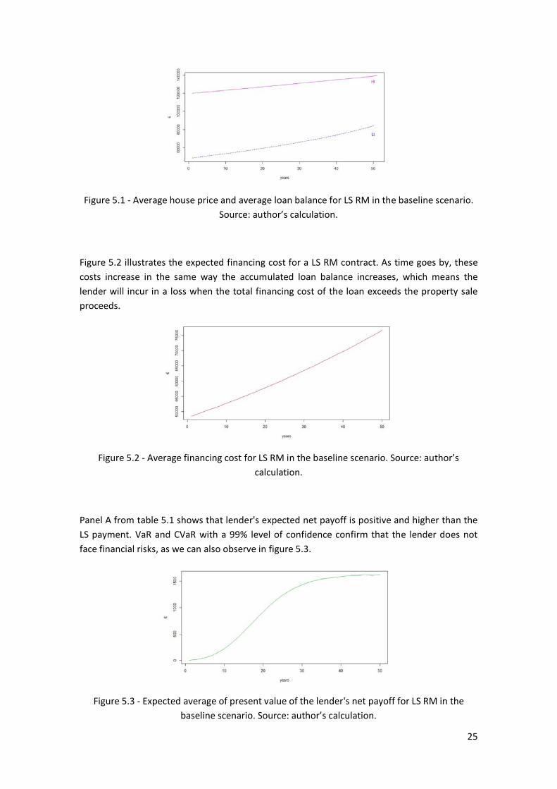
Figure 5.1 - Average house price and average loan balance for LS RM in the baseline

scenario. ........................................................................................................................... 25

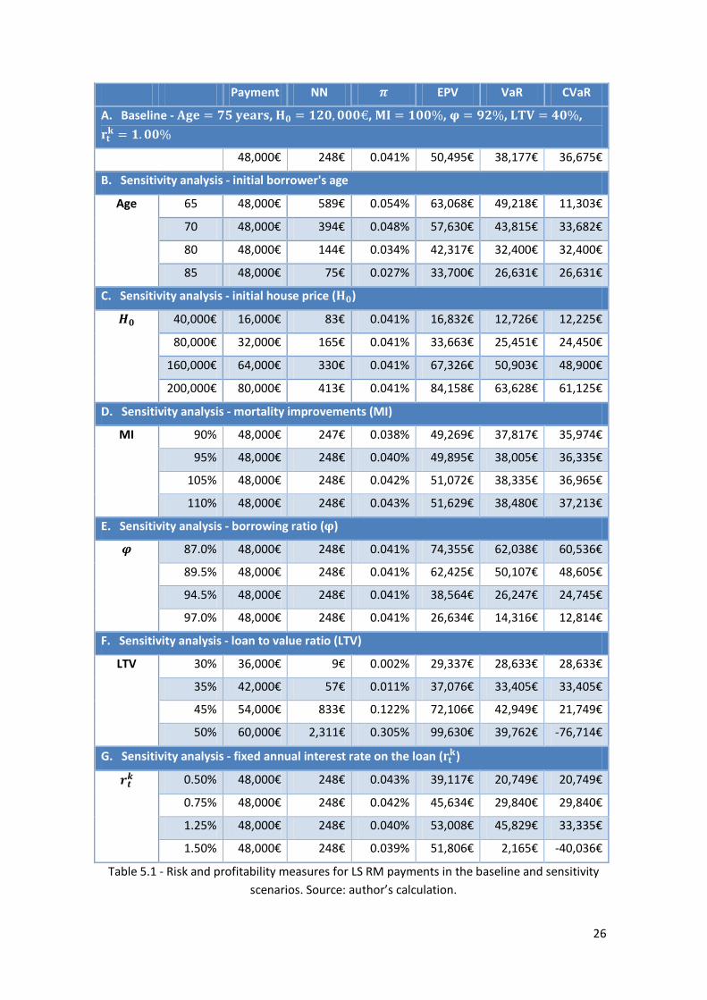
Figure 5.2 - Average financing cost for LS RM in the baseline scenario. ................................. 25

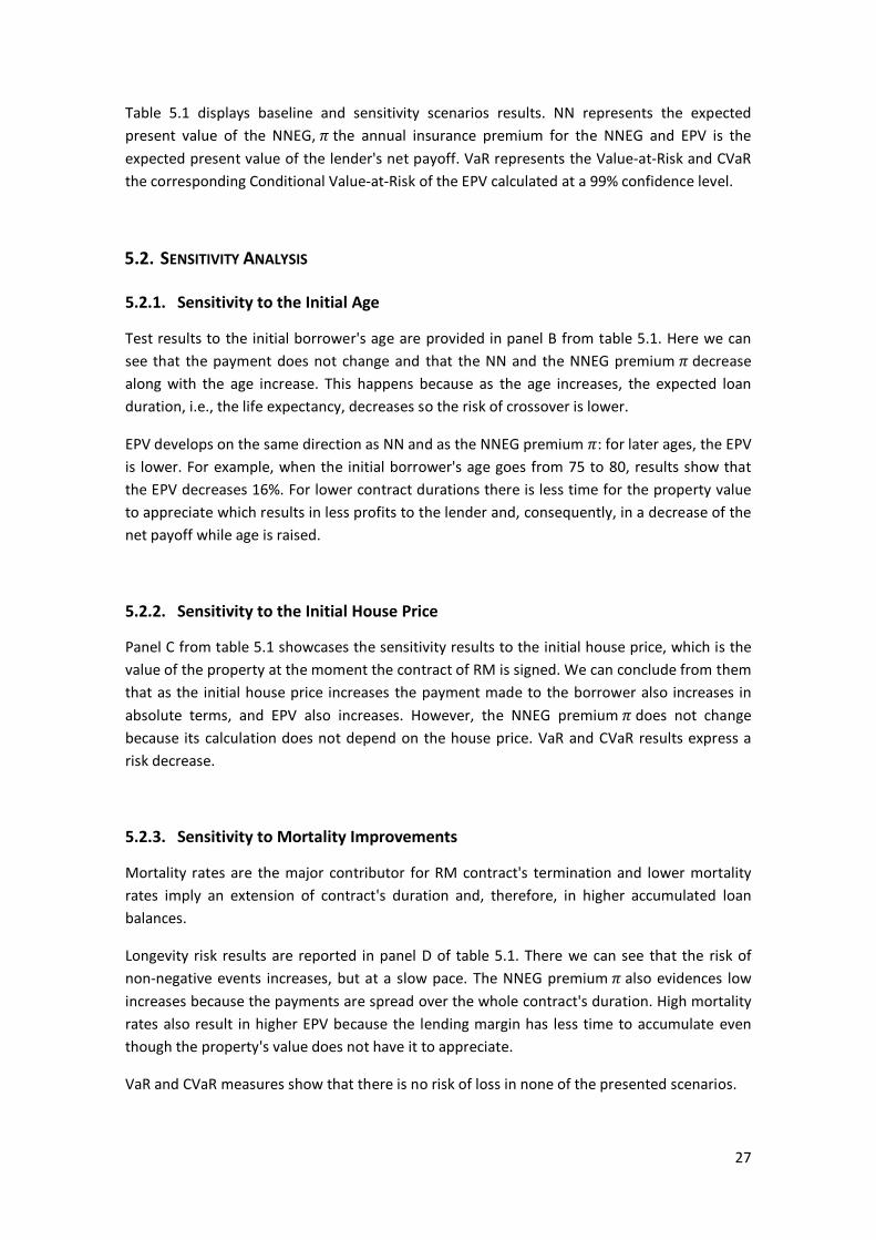
Figure 5.3 - Expected average of present value of the lender's net payoff for LS RM in the

baseline scenario. ............................................................................................................. 25

vii

LIST OF TABLES

Table 3.1 - RM contract particularities of contract designs around the world. ....................... 12

Table 4.1 - Life expectancy by age and cohort for the whole Portuguese population. ........... 19

Table 4.2 - VAR variables definition, source and frequency. ................................................... 20

Table 4.3 - Lag selection criterion according to R function VARorder. .................................... 22

Table 4.4 - Lag selection criterion according to R function VARorderI. ................................... 22

Table 4.5 - Estimated parameters of refined VAR (4) model. .................................................. 23

Table 5.1 - Risk and profitability measures for LS RM payments in the baseline and sensitivity

scenarios. .......................................................................................................................... 26

viii

LIST OF ABBREVIATIONS AND ACRONYMS

AIC Akaike Information Criterion

BIC Bayesian Information Criterion

CPI Consumer Price Index

CVaR Conditional Value-at-Risk

EPV Expected Present Value of the Lender's Net Payoff

GDP Gross Domestic Product

HPI House Price Index

HQC Hannan-Quinn Criterion

LS Lump Sum

LTV Loan to Value ratio

MI Mortality Improvements

MR Mortgage Rates

NN Expected Present Value of the No Negative Equity Guarantee

NNEG No Negative Equity Guarantee

r Euro Area Yields for 30 Years Maturity

RM Reverse Mortgage

VAR Vector Autoregressive

VaR Value-at-Risk

1

1. INTRODUCTION

The increase of the average lifetime and the consequent population ageing is a growing reality in many countries, mainly due to the healthcares advancements and to the better living conditions in general. However, the old age dependency level has been increasing and the monetary resources are not always enough to cover the healthcare expenses and/or to keep the same quality of life level (Vaz, 2014).

With the above mentioned in mind, many retirement products have been developed to address pensioners' risk of outliving their savings: life annuities, term annuities, lifetime phased withdrawals, lump sums or self-annuitization, just to name a few (Rocha et al., 2011). However all these products require that the retirees have financial liquid assets so that they can buy them.

Furthermore, many countries have high shares of house ownership among people with 65 years old or more. In 2013, according to the European Commission and to the Social Protection Committee, the European average of home ownership was 77%.

It is in this context of an old age population that is "house rich cash poor" that the financial institutions start to find adequate the commercialization of Reverse Mortgages (RM), also known as Lifetime Mortgages. A RM is the opposite of a typical mortgage, i.e., the homeowners receive a loan that corresponds to a fraction of the property's equity that is mainly calculated considering borrower's age and home's value. The loan can be delivered in the form of a Lump Sum (LS), regular payments, a line of credit or a combination of all three. The householder is entitled to live in his house until death or permanent move-out and, at that time, the heirs can pay the loan and get the house back, or the lender will execute the mortgage (Alai et al., 2013). This product has its origin in the United States but nowadays it can be found in many countries including Australia, Canada, Ireland, Japan, Spain and the United Kingdom.

During the last years many authors have been studying the applicability of this product. Débon Aucejo et al. (2013) studied the RM in the Spanish context using dynamic tables built for Spanish mortality. Davidoff & Welke (2007), Chen et al. (2010), Sherris et al. (2010), Alai et al. (2013) and Cho et al. (2013) discuss the many types of risks this product brings to the lenders (e.g. interest rate risk, inflation risk, house price risk, longevity risk).

Even though the RM is not yet developed in the Portuguese markets, in Martins (2011) we can find a brief description about the risks involved in a possible implementation of the product in Portugal and, more recently, Vaz (2014) analyses some relevant statistical indicators for this same implementation: population ageing indexes, old age dependency level, longevity, disposable income for the elderly and the average housing costs for Portuguese families. In this work we can also find a deterministic simulator that estimates the regular income stream to be received by the borrower. In both cases, the authors discuss how the RM product was implemented in some of the countries where it has already conquered a good share of the market.

2

This study extends the growing, but still few, literature on RM Portuguese market (see, e.g., Martins, 2011; Vaz, 2014). Considering the low-income level of most Portuguese retirees and the comparatively high level of home ownership, the aim of this paper is to discuss the valuation of standard RM contracts in Portugal.

If present trends continue and projected scenarios are confirmed, most Portuguese households working today will face a significant retirement funding gap. Projected public pension schemes deficits are expected to increase and replacement rates have been declining significantly as a result of parametric reforms in pension schemes. Portuguese public finance deficits are one of the highest public debt ratios in Europe. The implicit debt in pension schemes is estimated to more than 150% of annual GDP using an optimistic discount rate (Bravo et al., 2012, 2013, 2014). This study discusses whether RM can be used to fill at least some of the estimated retiree’s income gap.

Considering the high share of householders in Portugal and the quickly ageing of its population combined with the financial and structural problems in the social security system, we will understand that Portugal is a good candidate to develop this business, allowing the borrowers to recover and/or to reinforce their financial autonomy. And, it is because of all these motives that this study tries to explain and to analyse some of the risks involved in a Portuguese RM contract, aiming a near start of its broad commercialization.

The probability of loan's termination is one of the risks involved in this type of contracts because, from the lender's perspective, delayed termination results impact profits as these depend on financial and economic markets. RM contract termination can be triggered by borrower's death or move-out, and both depend on many factors like borrower's health or social status. Since we could not find data about elderly move-out rates in Portugal, in this study we will only model mortality rates. Following Bravo (2008), we adopt a stochastic mortality model (Poisson Lee-Carter age-period model) to project future mortality rates and to derive dynamic lifetables projections for the Portuguese population. This model is known for its good results, simplicity and easy interpretation of parameters (Lee, 2000; Booth et al., 2002). As stated in Coelho et al. (2010), this method "combines a demographic model, describing the historical change in mortality, a method for fitting the model and a time series model for the time component which is used for forecasting".

Besides termination risk, equity release products are also exposed to house price risk, mortgage rate risk and interest rate risk. Macroeconomic variables like gross domestic product (GDP) and consumer price index (CPI) also influence the dynamics of the three mentioned risks (see, for example, Abraham & Hendershott, 1994; Muellbauer & Murphy, 1997). Therefore, to capture the linear correlations in a multivariate time series system, we use a vector autoregressive (VAR) model to jointly model and project house price indexes (HPI), mortgage rates, interest rates, CPI and GDP like previously done in Alai et al. (2013).

Cash flows and actuarial present value of the lender's net payoff for LS RM, are calculated in different scenarios where the initial borrower's age, the initial house price, mortality rates, borrowing ratio, loan to value percentage and interest rate on the loan change. Value-at-Risk (VaR) and Conditional Value-at-Risk (CVaR) risk measures, at a 99% confidence level, are assessed to decide the risk-based capital level for solvency requirement.

3

We find that borrower's age at the beginning of the contract, as well as the mortality improvements, play a very important role on product's profitability and riskiness. Results show that for younger borrowers the profits are higher and that higher longevity rates allow property's value to appreciate but also imply higher financing costs for the lender. These results were produced under a financial context of low interest rates, so the model is very sensitive to shocks on loan interest rates since the mortgages rates and house appreciation do not change by the same amount. In all tested scenarios, LS RM contracts are expected to be profitable. Providers would only incur in loss in extreme scenarios, like in a real estate market collapse. However, lenders should always hold capital to face this risk.

Our results and literature review evidence the importance of offering these kind of financial products to ageing populations, like the Portuguese one. Both homeowners and investors would take advantages from this if the market development was stimulated by providing appropriate regulation and financial literacy to the consumers.

The remainder of this paper is organized as follows: section 2 introduces Portugal's demographic data and financial situation; section 3 presents the RM concept, the different types of contracts and describes their cash flows; section 4 sets out the RM LS pricing framework; section 5 reports the results; section 6 addresses our conclusions.

4

2. PORTUGAL: DEMOGRAPHIC DATA AND FINANCIAL SITUATION

As mentioned previously, the global ageing is affecting many countries and Portugal is not an exception. In 2013, according to Statistics Portugal, the life expectancy at birth was 83.0 years old for women and 77.2 for men, and a forecast for 2060 (based on 2012 data) estimated an increase to 89.88 years old for women and to 84.21 for men. The most recent data, from 2016, shows a life expectancy of 20.73 years for women and of 17.44 years for men at age 65.

Last Census data (collected in 2011) reveals that 19% of the total population is 65 years old or older, 60% of them live alone or exclusively accompanied by other old age people and 1 5� of the occupied residences in Portugal are solely inhabited by old age people. This data collection also demonstrates that the proportion of conventional dwellings that are owned by its own inhabitants is 73.24% and that its average useful area is 109 m2. Moreover, in May 2017 the average value from bank evaluation of living quarters in Portugal was 1,111€/m2, as reported by Statistics Portugal.

The Inquérito à Situação Financeira das Famílias (2012), a joint data collection of Bank of Portugal and Statistics Portugal made in 2010, revealed that non-financial assets in households’ assets represented 87.5% and the value of the household main residence corresponds to 54.6% of the total value of non financial assets, which points out the supremacy of a "brick-and-mortar saving account" for most families.

Regarding the financial situation of the Portuguese families, PORDATA shares that even though the average old age pension has been increasing 1 (5.002,70€/year in 2015), the final consumption expenditure in total of disposable income of families has also been increasing: in 1995 it was 90.8% and in 2014 it was 100.7%. Furthermore, according to Bank of Portugal's data, in the fourth quarter of 2016, Portugal had one of the lowest households liquid saving rates since 1999: 4.4% of the disposable income. The highest rate ever was registered in the second quarter of 1999 and it was 14.9%. It is also important to highlight that a study made by Alexandre et al. (2011) stated that in 2011, 90% of household's savings were generated by only 20% of the families.

Portugal has in recent years implemented several parametric pension reforms to cope with broken public finances and to strengthen the financial sustainability of pension systems by tightening eligibility and decreasing benefits (including nominal pension benefits during the Troika adjustment program). This has led to considerable decreases in the projected pension generosity over the coming decades. The benefit ratio of public (earnings related) pensions is expected to decline 15.8% in the forthcoming decades, from 59.3% in 2013 to only 43.4% in 2060 (European Comission, 2015). The projected decline in the public pension replacement rate between 2013 and 2060 is also massive, reaching only 30.7% in 2060. Reform measures tried to address mostly the fiscal sustainability concerns of pension systems. Social or political sustainability challenges were in most cases not considered and will emerge in countries like Portugal with a steep reduction in the generosity of pensions. Pension adequacy problems will be significant in the future (Bravo et al., 2013, 2014; Bravo, 2017).

1 2015 was the first year where a decrease in the average old pension was registered.

5

According to "Reforma das pensões: há soluções técnicas, não há solução política" by Corrêa de Aguiar (2015), besides the dangerous Portuguese demographic prognosis, financial and structural problems of the social security system have been causing a quickly decrease in taxpayers and beneficiaries' trust, but only 5.5% has occupational pension plans and 3.3% possesses voluntary private pension savings. In the same year, the European Commission along with the Social Protection Committee documented that, in 2013, 14.3% of the Portuguese householders aged 65 or more were at risk of poverty (against an European average of 13.1%2). Furthermore, the Portuguese share of financial assets3 on total gross assets for people with 65-74 years old is 12.2% and with 75+ years old is 15.5% (the average in Europe is 17.8% and 22.0%, respectively4).

Considering all these numbers and facts we realize that the reinforcement of the pensions system's third pillar has urged. Besides, with such an high rate of conventional dwellings that are owned by its own inhabitants, the development of Equity Release schemes in Portugal has all the necessary demographic and financial conditions to be successful.

2 Considers the data from 28 Member States: Austria, Belgium, Bulgaria, Croatia, Cyprus, Czech

Republic, Denmark, Estonia, Finland, France, Germany, Greece, Hungary, Ireland, Italy, Latvia, Lithuania, Luxemburg, Malta, the Netherlands, Poland, Portugal, Romania, Slovakia, Slovenia, Spain, Sweden and United Kingdom.

3 "Financial assets thereby include deposits (sight and saving accounts), mutual funds, bonds, shares, money owed to the households, value of voluntary pension plans and whole life insurance policies of household members and other financial assets item - which includes private non-self-employment businesses, assets in managed accounts and other types of financial assets." Source: European Commission (DG EMPL) and Social Protection Committee (SPC WG-AGE) (2015). The 2015 Pension Adequacy Report: current and future income adequacy in old age in the EU. Volume I. Luxembourg: Publications Office of the European Union.

4 Considers the data from 15 Member States: Austria, Belgium, Cyprus, Finland, France, Germany, Greece, Italy, Luxembourg, Malta, the Netherlands, Portugal, Slovakia, Slovenia and Spain.

6

3. REVERSE MORTGAGE

3.1. THE CONCEPT

As stated in Reifner et al. (2007), an Equity Release scheme is the transformation of an owner occupied dwelling into cash for private retirement pensions while the owner can continue to live in it. These schemes can be offered as a:

• Loan Model: consists on the provision of a loan to be paid once the dwelling is sold out or once it is paid by the heirs in case they decide to keep the house for them. This model is also known by RM or by Lifetime Mortgage.

• Sale Model: implies the immediate sale of the property but the householder keeps the right to live in there until his death or permanent move-out.

This work will only address the study of the Loan Model which from now on will be referred to as RM. The description below corresponds to a general overview about the product, but different features may be found in the market.

According to Cho et al. (2013), Débon Aucejo & Montes (2013) and Shao et al. (2014), under a RM scheme the borrower (which can be a single person or a couple) continues to live in his home and the lender advances cash and takes a mortgage over the property5. As so, over the years, the householder's equity in the house will continue to decrease as the interest accumulates and, implicitly, the same will happen to his legacy. This loan can be delivered in the form of a LS, an income stream, a line of credit or a combination of all three, and the agreed interest rates can be fixed or variable. Its maximum amount calculation is based on borrower's age and gender and on dwelling's value. Usually, early payments or refinancing are allowed, but with the drawback of having to pay penalty charges.

When the borrower dies or decides to permanently move-out, the contract finishes and at that time the loan and the accumulated interest is paid by the heirs, if they choose to keep the house, or with the property sale proceeds. If the sale proceeds exceed the outstanding loan amount plus transaction costs, the remaining goes to the borrower's heritage but, if on the contrary the sale proceeds do not cover the whole debt (known as "cross-over risk"), typically, neither the borrower or the heirs have to pay the difference because these contracts are non-recourse, so the lender is responsible for the shortfalls and the heirs are protected from the downside risk in future house prices. Some regulators even require a clause contract stating the "No Negative Equity Guarantee" (NNEG), which means that no other asset besides the property needs to be provided to pay the loan amount. This guarantee is subject to the borrower's commitment of doing a proper maintenance of the dwelling and to take care of all expenses with the property.

5 The contract will only be celebrated if there are no mortgages on the house. In case it exists, it

should be a residual amount so that it can be amortized in the loan or immediately paid by the borrower.

7

Despite of all the forms that a RM contract can assume, it always carries interrelated risks to the product's provider:

• Interest rate risk; • House price risk; • Termination risk.

Additionally, if the borrower opts for an agreement that pays an inflation-indexed income stream instead of fixed payments, then the provider is also vulnerable to the inflation rate risk.

To better understand the interrelationship of all these risks, suppose that a contract finishes later than the expected and that the economy is experiencing an environment of high interest rates: the probability of cross-over risk increases in these kind of situations, especially if the house prices are declining and/or if the contract implies regular inflation-indexed payments during a period of high inflation rates.

As pointed out above, the contract establishes that the maintenance of the house is a borrower's duty. This topic is faced as a risk for the lender but it will not be discussed in this document. For further detail please refer to Miceli & Sirmans (1994), Chinloy & Megbolugbe (1994), Shiller & Weiss (2000) or Davidoff & Welke (2007).

It is also important to underline that RM contracts also carry some costs and disadvantages for the borrower. Usually, it is subject to higher interest rates when compared to other mortgage products and some fees are charged at the contract's setup, during and at its termination. Also, the maintenance of the dwelling must be done as required by the lender, all outgoings are paid by the householder (including insurance) and he cannot leave the property for more than 6-12 months without permission nor have non-approved residents. Selling, leasing and renovating activities are also subject to lender's approval.

3.2. REVERSE MORTGAGE CASH FLOWS

This section describes in detail the cash flows of a RM contract structure as considered in Cho et al. (2013).

We model the cash flows on a quarterly basis and consider that the contracts are non-recourse, i.e., they require the NNEG.

3.2.1. Lump Sum Reverse Mortgages

For RM that pay out the whole loan amount at the beginning of the contract, we can state the following:

𝑃𝐿𝑆 = 𝐿0𝐿𝑆 ( 1 )

8

𝐿𝑡𝐿𝑆 = 𝐿0𝐿𝑆exp ��(𝑟𝑖𝜅 + 𝜋)𝑡

𝑖=0

� ( 2 )

where 𝑃𝐿𝑆 is the LS payment made to the borrower, 𝐿𝑡𝐿𝑆 is the outstanding loan amount at time 𝑡 and 𝑟𝑖𝜅 and 𝜋 stand for the variable mortgage rate and the risk-adjusted premium rate for the NNEG, by which the loan balance increases each quarter, respectively.

Lender's financing cost for a LS RM loan at time 𝑡 is given by:

𝐶𝑡𝐿𝑆 = 𝜑𝐿0𝐿𝑆exp ��𝑟𝑖

(1)𝑡

𝑖=0

�+ (1− 𝜑)𝐿0𝐿𝑆 ( 3 )

where 𝜑 is the borrowing ratio and 𝑟𝑖(1) is the short rate at which the borrowed capital

accumulates.

The expected present value of the lender's net payoff from the LS RM is given by:

𝐸𝑃𝑉𝐿𝑆 = � 𝑞𝑥,𝑡

𝑐𝜔−𝑥−1

𝑡=0

exp �−�𝑟𝑖(1)

𝑡

𝑖=0

� [min(𝐿𝑡𝐿𝑆, (1− 𝛾)𝐻𝑡) − 𝐶𝑡𝐿𝑆] ( 4 )

where 𝜔 is the maximum attainable age of the borrower, 𝑞𝑥,𝑡𝑐 is the probability of the loan

termination for a borrower initially aged 𝑥, 𝛾 represents the assumed proportional transaction cost of selling the house and 𝐻𝑡 stands for the value of the property at time 𝑡.

This payoff is only received at loan termination (at time 𝑇) and it cannot exceed the property's sale proceeds. As mentioned before, 𝑇 is determined by borrower's health condition and prepayment or by refinancing decisions, so it is random.

3.2.2. Income Stream Reverse Mortgages

This type of RM pays regular amounts to the borrower until contract's termination. These amounts can be fixed or inflation-indexed.

The loan amount is very low at the beginning of the contract and increases over time according to the accrued variable mortgage rate (𝑟𝑖𝜅), the risk-adjusted premium rate for the NNEG (𝜋) and each new payment made by the lender to the borrower.

In order to compare the payments made to the borrower in a LS RM and in an income stream RM with fixed payments we can have a look at equation (5):

𝑃𝐿𝑆 = 𝑃𝐼𝑆 � 𝑝𝑥,𝑡𝑐

𝜔−𝑥−1

𝑡=0

exp �−𝑟0(𝑡)𝑡� ( 5 )

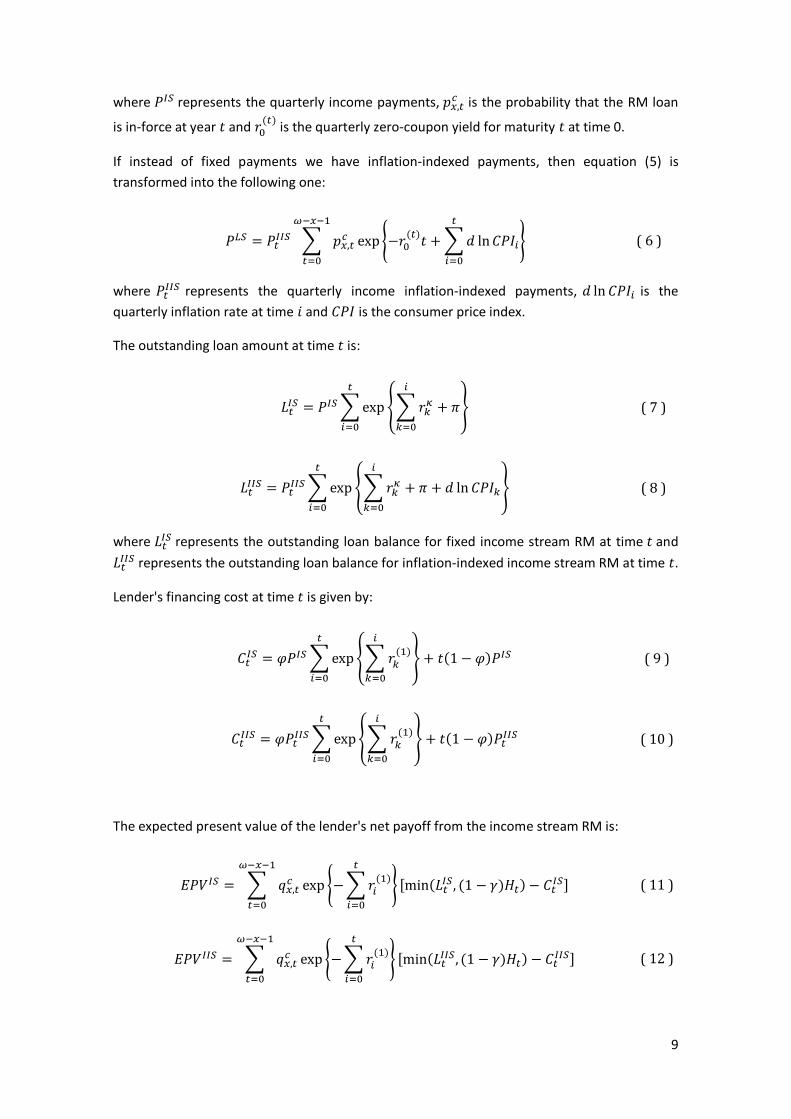
9

where 𝑃𝐼𝑆 represents the quarterly income payments, 𝑝𝑥,𝑡𝑐 is the probability that the RM loan

is in-force at year 𝑡 and 𝑟0(𝑡) is the quarterly zero-coupon yield for maturity 𝑡 at time 0.

If instead of fixed payments we have inflation-indexed payments, then equation (5) is transformed into the following one:

𝑃𝐿𝑆 = 𝑃𝑡𝐼𝐼𝑆 � 𝑝𝑥,𝑡𝑐

𝜔−𝑥−1

𝑡=0

exp �−𝑟0(𝑡)𝑡 + �𝑑 ln𝐶𝑃𝐼𝑖

𝑡

𝑖=0

� ( 6 )

where 𝑃𝑡𝐼𝐼𝑆 represents the quarterly income inflation-indexed payments, 𝑑 ln𝐶𝑃𝐼𝑖 is the quarterly inflation rate at time 𝑖 and 𝐶𝑃𝐼 is the consumer price index.

The outstanding loan amount at time 𝑡 is:

𝐿𝑡𝐼𝑆 = 𝑃𝐼𝑆� exp��𝑟𝑘𝜅 + 𝜋𝑖

𝑘=0

�𝑡

𝑖=0

( 7 )

𝐿𝑡𝐼𝐼𝑆 = 𝑃𝑡𝐼𝐼𝑆� exp��𝑟𝑘𝜅 + 𝜋 + 𝑑 ln𝐶𝑃𝐼𝑘

𝑖

𝑘=0

�𝑡

𝑖=0

( 8 )

where 𝐿𝑡𝐼𝑆 represents the outstanding loan balance for fixed income stream RM at time 𝑡 and 𝐿𝑡𝐼𝐼𝑆 represents the outstanding loan balance for inflation-indexed income stream RM at time 𝑡.

Lender's financing cost at time 𝑡 is given by:

𝐶𝑡𝐼𝑆 = 𝜑𝑃𝐼𝑆� exp�� 𝑟𝑘(1)

𝑖

𝑘=0

�+ 𝑡(1− 𝜑)𝑃𝐼𝑆𝑡

𝑖=0

( 9 )

𝐶𝑡𝐼𝐼𝑆 = 𝜑𝑃𝑡𝐼𝐼𝑆� exp�� 𝑟𝑘(1)

𝑖

𝑘=0

�𝑡

𝑖=0

+ 𝑡(1 − 𝜑)𝑃𝑡𝐼𝐼𝑆 ( 10 )

The expected present value of the lender's net payoff from the income stream RM is:

𝐸𝑃𝑉𝐼𝑆 = � 𝑞𝑥,𝑡𝑐

𝜔−𝑥−1

𝑡=0

exp �−�𝑟𝑖(1)

𝑡

𝑖=0

� [min(𝐿𝑡𝐼𝑆, (1 − 𝛾)𝐻𝑡)− 𝐶𝑡𝐼𝑆] ( 11 )

𝐸𝑃𝑉𝐼𝐼𝑆 = � 𝑞𝑥,𝑡𝑐

𝜔−𝑥−1

𝑡=0

exp �−�𝑟𝑖(1)

𝑡

𝑖=0

� [min(𝐿𝑡𝐼𝐼𝑆, (1 − 𝛾)𝐻𝑡) − 𝐶𝑡𝐼𝐼𝑆] ( 12 )

10

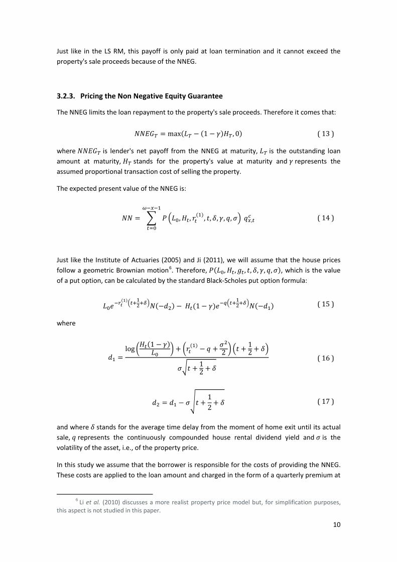
Just like in the LS RM, this payoff is only paid at loan termination and it cannot exceed the property's sale proceeds because of the NNEG.

3.2.3. Pricing the Non Negative Equity Guarantee

The NNEG limits the loan repayment to the property's sale proceeds. Therefore it comes that:

𝑁𝑁𝐸𝐺𝑇 = max(𝐿𝑇 − (1 − 𝛾)𝐻𝑇 , 0) ( 13 )

where 𝑁𝑁𝐸𝐺𝑇 is lender's net payoff from the NNEG at maturity, 𝐿𝑇 is the outstanding loan amount at maturity, 𝐻𝑇 stands for the property's value at maturity and 𝛾 represents the assumed proportional transaction cost of selling the property.

The expected present value of the NNEG is:

𝑁𝑁 = � 𝑃�𝐿0,𝐻𝑡 , 𝑟𝑡(1), 𝑡,𝛿, 𝛾,𝑞, 𝜎� 𝑞𝑥,𝑡

𝑐𝜔−𝑥−1

𝑡=0

( 14 )

Just like the Institute of Actuaries (2005) and Ji (2011), we will assume that the house prices follow a geometric Brownian motion6. Therefore, 𝑃(𝐿0,𝐻𝑡 ,𝑔𝑡 , 𝑡, 𝛿, 𝛾, 𝑞,𝜎), which is the value of a put option, can be calculated by the standard Black-Scholes put option formula:

𝐿0𝑒−𝑟𝑡

(1)�𝑡+12+𝛿�𝑁(−𝑑2) − 𝐻𝑡(1− 𝛾)𝑒−𝑞�𝑡+12+𝛿�𝑁(−𝑑1) ( 15 )

where

𝑑1 =log �𝐻𝑡(1 − 𝛾)

𝐿0� + �𝑟𝑡

(1) − 𝑞 + 𝜎22 � �𝑡 + 1

2 + 𝛿�

𝜎�𝑡 + 12 + 𝛿

( 16 )

𝑑2 = 𝑑1 − 𝜎�𝑡 +12

+ 𝛿 ( 17 )

and where 𝛿 stands for the average time delay from the moment of home exit until its actual sale, 𝑞 represents the continuously compounded house rental dividend yield and 𝜎 is the volatility of the asset, i.e., of the property price.

In this study we assume that the borrower is responsible for the costs of providing the NNEG. These costs are applied to the loan amount and charged in the form of a quarterly premium at

6 Li et al. (2010) discusses a more realist property price model but, for simplification purposes,

this aspect is not studied in this paper.

11

a fixed rate 𝜋 but only paid at the termination of the contract. Its expected present value is given by:

𝑀𝐼𝑃 = 𝜋 � ��𝐿0𝑒𝑟𝑡𝑘𝑡� �𝑒∑ 𝑟𝑖

(1)𝑡𝑖=0 �𝑝𝑥,𝑡

𝑐 � 𝜔−𝑥−1

𝑡=0

( 18 )

The NNEG premium 𝜋 is calculated by setting 𝑁𝑁 = 𝑀𝐼𝑃. As a result, the NNEG amount will depend on the type of reverse mortgage contract: LS or income stream, since it depends on how the loan balance accumulates.

3.3. REVERSE MORTGAGES AROUND THE WORLD

This product has already conquered a good market portion in some countries, including Australia, Canada, Ireland, Japan, Spain, the United Kingdom (UK) and the United States of America (USA), just to name a few.

For some countries, we summarize below the most relevant particularities of these contract designs according to Vaz (2014). The following definitions should be considered to better understand table 3.1:

• Minimum age - minimum age to require a RM contract. Usually, if there is more than one borrower (e.g. a couple) the age of the youngest should be considered;

• Upper limit - maximum limit of the loan;

• Lower limit - minimum limit of the loan;

• NNEG? - is the lender required to offer the NNEG?;

• Entities/Programs - entities or programs that offer special contract conditions or offer counseling;

• Others - any other particularity that we believe we should draw attention to.

Note that these criteria are valid for most cases but we can find variations.

If the chart is filled in with "-" it means we do not have information about it.

Detailed descriptions can be found in Alai et al. (2013), Herranz González (2006), Hosty et al. (2008) and Chen et al. (2010) for RM contracts in Australia, Spain, UK and USA, respectively.

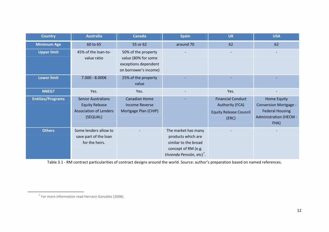
12

Country Australia Canada Spain UK USA

Minimum Age 60 to 65 55 or 62 around 70 62 62

Upper limit 45% of the loan-to-value ratio

50% of the property value (80% for some

exceptions dependent on borrower's income)

- - -

Lower limit 7.000 - 8.000€ 25% of the property value

- - -

NNEG? Yes. Yes. - Yes. -

Entities/Programs Senior Australians Equity Release

Association of Lenders (SEQUAL)

Canadian Home Income Reverse

Mortgage Plan (CHIP)

- Financial Conduct Authority (FCA)

Equity Release Council (ERC)

Home Equity Conversion Mortgage -

Federal Housing Administration (HECM -

FHA)

Others Some lenders allow to save part of the loan

for the heirs.

- The market has many products which are similar to the broad concept of RM (e.g.

Vivienda Pensión, etc)7.

- -

Table 3.1 - RM contract particularities of contract designs around the world. Source: author’s preparation based on named references.

7 For more information read Herranz González (2006).

13

4. REVERSE MORTGAGE PRICING FRAMEWORK

4.1. STOCHASTIC MORTALITY MODEL

In 1992 the Lee-Carter method was proposed by Lee and Carter to obtain dynamic lifetables and since then it has been used by many authors to study the mortality in some countries, such as Australia (Booth & Tickle, 2003), Austria (Carter & Prkawetz, 2001), Belgium (Brouhns et al., 2002), Canada (Lee & Nault, 1993), Chile (Lee & Rofman, 1994), England and Wales (Renshaw & Haberman, 2003), Japan (Wilmoth, 1996), Portugal (Bravo, 2008) and Spain (Guillen & Vidiella-i-Anguera, 2005; Debón et al., 2008). It is known for its good results, simplicity and easy interpretation of parameters (Lee, 2000; Booth et al., 2002). As stated in Coelho et al. (2010), this method "combines a demographic model, describing the historical change in mortality, a method for fitting the model and a time series model for the time component which is used for forecasting".

The model is given by the following function:

𝑚𝑥,𝑡 = exp�𝛼𝑥 + 𝛽𝑥𝑘𝑡 + 𝜀𝑥,𝑡� ( 19 )

⇔ ln�𝑚𝑥,𝑡� = 𝛼𝑥 + 𝛽𝑥𝑘𝑡 + 𝜀𝑥,𝑡 ( 20 )

where 𝑚𝑥,𝑡 represents the central mortality rate at age 𝑥 and at year 𝑡, 𝛼𝑥 is a vector of age specific constants to describe the overall pattern of mortality by age, 𝛽𝑥 is a vector of age specific constants to describe the overall pattern of deviations from the general level of mortality over time, i.e., when 𝑘𝑡 varies, 𝑘𝑡 represents the trend of mortality in the studied period and 𝜀𝑥,𝑡 is the residual term with average 0 and variance 𝜎𝜀2 that reflects historical fluctuations at particular ages that are not captured by the model.

The method requires the following two constraints in order to get one single solution:

� 𝛽𝑥

𝑥max

𝑥=𝑥min

= 1 ( 21 )

� 𝑘𝑡

𝑡max

𝑡=𝑡min

= 0 ( 22 )

And as a result of (21) and (22), 𝛼𝑥 is the average of ln�𝑚𝑥,𝑡� over time.

The least-squares estimation via singular value decomposition of the ln�𝑚𝑥,𝑡� matrix is the main statistical tool of Lee & Carter (1992) and, in order to match the fitted deaths with the total deaths observed in each year, they included an adjustment to the estimated 𝑘𝑡. The authors assume that 𝛼𝑥 and 𝛽𝑥 are constants throughout time and predict 𝑘𝑡 values using a standard ARIMA univariate time series model.

14

Among the disadvantages, Lee-Carter method is criticized for considering that residual terms 𝜀𝑥,𝑡 follow a normal distribution with constant variance, which does not correspond to the reality because the observed mortality rate's logarithm varies much more at older ages (see, for example, Booth and Tickle, 2008; Lee and Miller, 2001).

In Brounhs et al. (2002) the authors overcame this by developing a different approach to mortality forecasting based on heteroskedastic Poisson error structures: Poisson-Lee-Carter model. This model replaces the ordinary least-squares by Poisson regression for the death counts and estimates model parameters by maximizing a Poisson log-likelihood8.

Poisson Lee-Carter Model assumes "that the age-specific forces of mortality are constant within bands of age and time (...) but allowed to vary from one band to the next" (Coelho et al., 2010), i.e.:

𝜇𝑥+𝜉,𝑡+𝜏 = 𝜇𝑥,𝑡 , 0 ≤ 𝜉 , 𝜏 < 1 ( 23 )

where 𝑥 represents the age and 𝑡 the calendar year. This assumption allows us to estimate 𝜇𝑥,𝑡:

𝜇𝑥,𝑡 = 𝑚𝑥,𝑡 =𝐷𝑥,𝑡

𝐸𝑥,𝑡 ( 24 )

where 𝐷𝑥,𝑡 represents the number of deaths at age 𝑥 and year 𝑡, and 𝐸𝑥,𝑡 those who are exposed to risk at age 𝑥 and year 𝑡.

Brounhs et al. (2002) assumes that

𝐷𝑥,𝑡 ~ 𝑃𝑜𝑖𝑠𝑠𝑜𝑛 (𝜇𝑥,𝑡 𝐸𝑥,𝑡) ( 25 )

with

𝜇𝑥,𝑡 = exp(𝛼𝑥 + 𝛽𝑥𝑘𝑡) ( 26 )

Thus, the log-bilinear structure for (26) is preserved and the assumptions on the error term 𝜀𝑥,𝑡 have changed from a Normal law to a Poisson for 𝑑𝑥,𝑡. Parameters 𝛼𝑥, 𝛽𝑥 and 𝑘𝑡 are now estimated by maximizing (27) but its interpretation is the same as before:

L(𝛼𝑥,𝛽𝑥,𝑘𝑡) = � � �𝑑𝑥,𝑡(𝛼𝑥 + 𝛽𝑥𝑘𝑡) − 𝐸𝑥,𝑡 exp(𝛼𝑥 + 𝛽𝑥𝑘𝑡)� + 𝑐𝑡𝑚𝑎𝑥

𝑡=𝑡𝑚𝑖𝑛

𝑥𝑚𝑎𝑥

𝑥=𝑥𝑚𝑖𝑛

( 27 )

where 𝑐 is a constant. Because of the presence of log-bilinear term 𝛽𝑥𝑘𝑡 in (26), the model was estimated using an algorithm developed by Goodman (1979) 9. To guarantee that the

8 Details about its advantages can be found in Coelho et al. (2010). 9 Details about the procedure can be found in Brouhns et al. (2002).

15

parameters 𝛼𝑥, 𝛽𝑥 and 𝑘𝑡, generated by the log-likelihood function in (27), verify the model constraints, a reparameterization of the model is needed. The age-sex-specific mortality rates are forecasted using the time series methods described previously.

The death rates projected by the Poisson Lee-Carter model have an unsatisfactory asymptotic behavior and some empirical studies on the Portuguese population conducted on this model show a decrease on the mortality trend (i.e., on 𝑘�𝑡) and higher deviations on the general level of mortality over time (i.e., on 𝛽𝑥). Therefore, the extrapolation of 𝑘�𝑡 by using time-series methods with long term horizons will result on death rates close to zero:

lim𝑘�→+∞

exp�𝛼�𝑥 + �̂�𝑥𝑘�𝑡� = 0 ( 28 )

with 𝛽𝑥 > 0 and finite 𝛼𝑥. However, according to life science, this is very unlikely to happen to the humanity and that is why we have the need to choose a reasonable upper limit to life span when projecting mortality lifetables, which means we will have to admit that humans longevity has natural limits.

Following this research started by Bourgeois-Pichat (1952), Bravo (2008) developed an extension of the Poisson Lee-Carter model where there is a convergence of longevity improvements. To incorporate a limit life table on the Poisson Lee-Carter model we need to replace (25) by (29), where 𝜇𝑥𝑙𝑖𝑚 represents the instantaneous death rates and 𝑞𝑥𝑙𝑖𝑚 the probabilities of death corresponding to this limit lifetable

𝐷𝑥,𝑡~𝑃𝑜𝑖𝑠𝑠𝑜𝑛 (𝐸𝑥,𝑡(𝜇𝑥,𝑡𝑙𝑖𝑚 + 𝜇𝑥,𝑡

𝑎𝑑)) ( 29 )

with

𝜇𝑥,𝑡𝑎𝑑 = exp(𝛼𝑥 + 𝛽𝑥𝑘𝑡) ( 30 )

and the inevitable identification restrictions.

Again, with these assumptions, parameter estimates are given by maximizing the log-likelihood function, using an iterative algorithm adapted from Goodman (1979). Lastly, to comply with the identification constraints, the initial parameter estimates generated by the algorithm are adjusted. Details about this procedure can be found in Bravo (2008).

At more advanced ages, the number of living individuals is significantly lower than at early ages. This scarcity of data influences the estimated mortality rates causing big random fluctuations and bringing unreliable results. Bad quality of data is also a cause for misleading forecasts. To overcome this issue, during the construction of the tables, the crude estimations were smoothed, and all fluctuations were removed.

Denuit & Goderniaux (2005) proposed a method to apply directly to crude death probabilities, where, as a starting point, a maximum age for the life table must be defined. The following log--quadratic regression model is fitted by weighted-least squares to age-specific death probabilities observed at oldest ages:

16

ln(𝑞�𝑥) = 𝑎 + 𝑏𝑥 + 𝑐𝑥2 + 𝜀𝑥 ( 31 )

where 𝜀𝑥 follows a Normal distribution with average 0 and variance 𝜎2. Constraints (32) and (33) have to be considered in equation (31). These will transform (31) into (34):

𝑞𝑥max = 1 ( 32 )

𝑞′𝑥max = 0 ( 33 )

ln(𝑞�𝑥) = (𝑥max2 − 2𝑥(𝑥max) + 𝑥2)𝑐 + 𝜀𝑥 , 𝜀𝑥 ∼ 𝑁(0, 𝜎2) ( 34 )

The 𝑥max should be chosen according to the one that better describes the data. The determination of the age from which the adjusted estimate is applied is one of the most criticized aspects of this model. Denuit & Goderniaux (2005) suggest determining it so that in the age range of [50, 85] the regression coefficient 𝑅2 is maximized. It is also important to avoid strong discontinuities between gross and adjusted mortality probabilities. Hence, one of the recommendations is to replace initial estimates 𝑞�𝑥 by a 5-year geometric average of the death probabilities around ages 𝑥 = 𝑥0 − 5, 𝑥0 − 4, ..., 𝑥0 + 4, 𝑥0 + 5.

For more details about the methodology used for the construction of prospective lifetables refer to Bravo & Silva (2012).

4.1.1. Application to Portuguese Mortality Data

The Human Mortality Database website provides the observed number of deaths (by age and year of death) and of the observed population size at December 31st of each year for the Portuguese population, corresponding to the period 1940-2015 and a range of ages from 0 to 110. Due to some data issues in the data prior to 1981 (including considerable age heaping) the analysed period is 1981-2015.

The crude death probabilities (𝑞x,t) were obtained by doing:

𝑞x,t = 1 − exp�𝑚𝑥,𝑡� ( 35 )

Figure 4.1 represents the mortality trend for the Portuguese population during 1981-2015. It can be seen that there was a mortality decline at young ages due to infection diseases and also at old ages, mainly due to medical advances.

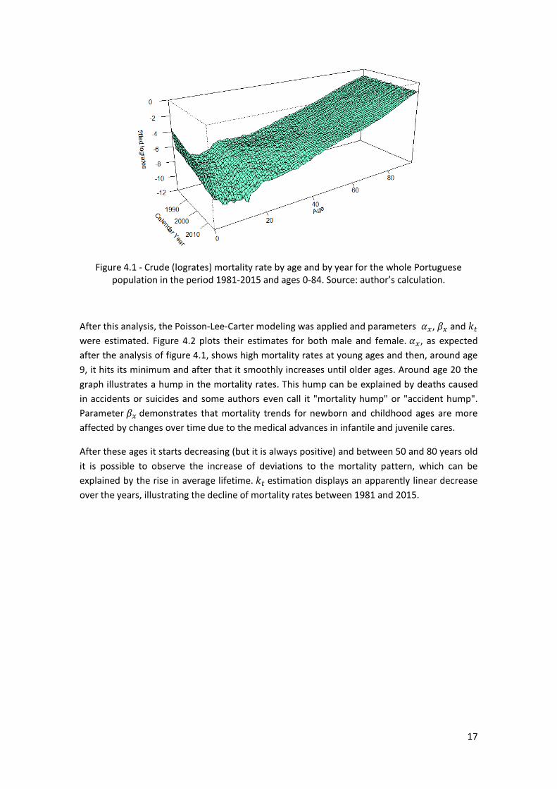
17

Figure 4.1 - Crude (logrates) mortality rate by age and by year for the whole Portuguese population in the period 1981-2015 and ages 0-84. Source: author’s calculation.

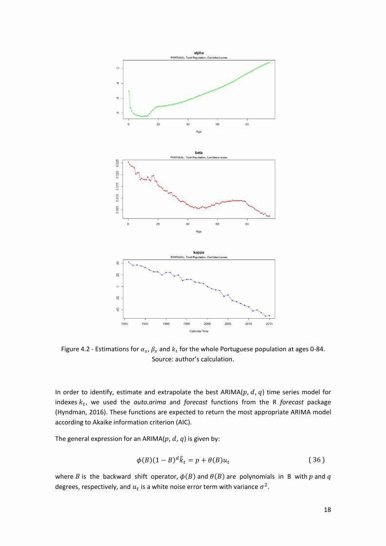
After this analysis, the Poisson-Lee-Carter modeling was applied and parameters 𝛼𝑥, 𝛽𝑥 and 𝑘𝑡 were estimated. Figure 4.2 plots their estimates for both male and female. 𝛼𝑥, as expected after the analysis of figure 4.1, shows high mortality rates at young ages and then, around age 9, it hits its minimum and after that it smoothly increases until older ages. Around age 20 the graph illustrates a hump in the mortality rates. This hump can be explained by deaths caused in accidents or suicides and some authors even call it "mortality hump" or "accident hump". Parameter 𝛽𝑥 demonstrates that mortality trends for newborn and childhood ages are more affected by changes over time due to the medical advances in infantile and juvenile cares.

After these ages it starts decreasing (but it is always positive) and between 50 and 80 years old it is possible to observe the increase of deviations to the mortality pattern, which can be explained by the rise in average lifetime. 𝑘𝑡 estimation displays an apparently linear decrease over the years, illustrating the decline of mortality rates between 1981 and 2015.

18

Figure 4.2 - Estimations for 𝛼𝑥, 𝛽𝑥 and 𝑘𝑡 for the whole Portuguese population at ages 0-84. Source: author’s calculation.

In order to identify, estimate and extrapolate the best ARIMA(𝑝, 𝑑, 𝑞) time series model for indexes 𝑘𝑡, we used the auto.arima and forecast functions from the R forecast package (Hyndman, 2016). These functions are expected to return the most appropriate ARIMA model according to Akaike information criterion (AIC).

The general expression for an ARIMA(𝑝, 𝑑, 𝑞) is given by:

𝜙(𝐵)(1 − 𝐵)𝑑𝑘�𝑡 = 𝑝 + 𝜃(𝐵)𝑢𝑡 ( 36 )

where 𝐵 is the backward shift operator, 𝜙(𝐵) and 𝜃(𝐵) are polynomials in B with 𝑝 and 𝑞 degrees, respectively, and 𝑢𝑡 is a white noise error term with variance 𝜎2.

19

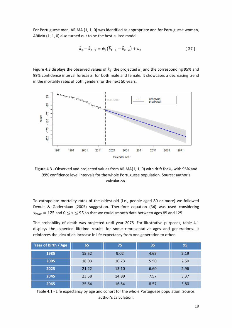
For Portuguese men, ARIMA (1, 1, 0) was identified as appropriate and for Portuguese women, ARIMA (1, 1, 0) also turned out to be the best-suited model.

𝑘�𝑡 − 𝑘�𝑡−1 = 𝜙1�𝑘�𝑡−1 − 𝑘�𝑡−2� + 𝑢𝑡 ( 37 )

Figure 4.3 displays the observed values of 𝑘𝑡, the projected 𝑘�𝑡 and the corresponding 95% and 99% confidence interval forecasts, for both male and female. It showcases a decreasing trend in the mortality rates of both genders for the next 50 years.

Figure 4.3 - Observed and projected values from ARIMA(1, 1, 0) with drift for 𝑘𝑡 with 95% and 99% confidence level intervals for the whole Portuguese population. Source: author’s

calculation.

To extrapolate mortality rates of the oldest-old (i.e., people aged 80 or more) we followed Denuit & Goderniaux (2005) suggestion. Therefore equation (34) was used considering 𝑥max = 125 and 0 ≤ 𝑥 ≤ 95 so that we could smooth data between ages 85 and 125.

The probability of death was projected until year 2075. For illustrative purposes, table 4.1 displays the expected lifetime results for some representative ages and generations. It reinforces the idea of an increase in life expectancy from one generation to other.

Year of Birth / Age 65 75 85 95

1985 15.52 9.02 4.65 2.19

2005 18.03 10.73 5.50 2.50

2025 21.22 13.10 6.60 2.96

2045 23.58 14.89 7.57 3.37

2065 25.64 16.54 8.57 3.80

Table 4.1 - Life expectancy by age and cohort for the whole Portuguese population. Source: author’s calculation.

20

Summarily, these results show a continuous decline in mortality rates, especially at younger ages.

For a more detailed analysis refer to Bravo (2010).

4.2. VAR MODEL

In order to jointly model and project future HPI, mortgage rates, interest rates, CPI and GDP a VAR model is used. This kind of model intends to capture the linear correlations in a multivariate time series system. Its flexibility and simplicity popularized the model.

The joint modeling of house prices indexes (which will help us to predict future property's sale returns), mortgage rates and interest rates is especially important for variable interest rate RM, because many studies confirm that these three variables are strongly correlated (Alai et al., 2013). Furthermore, macroeconomic variables can also influence the dynamics of the three above mentioned variables (see, for example, Abraham & Hendershott, 1994; Muellbauer & Murphy, 1997) and that is why we included the GDP and the CPI in our VAR framework.

The raw data was accessed in August 2016 and is summarized in table 4.2. The longest period available for all variables was January 2009 - March 2016, which is what is being used in this study. Also, the frequency was different between variables, so we had to convert all daily and monthly series into quarterly ones.

Variable Definition Source Frequency

HPI House Price Index Stats Portugal Quarterly

GDP Gross Domestic Product Stats Portugal Quarterly

CPI Consumer Price Index Stats Portugal Monthly

MR Mortgage Rates Stats Portugal Monthly

r Euro area yields for 30 years maturity European Central Bank Daily

Table 4.2 - VAR variables definition, source and frequency.

HPI, GPD and CPI were converted into continuously compounding quarterly growth rates to keep consistency across all data set. In figure 4.4, we can see how our data progressed during the 29 quarters studied.

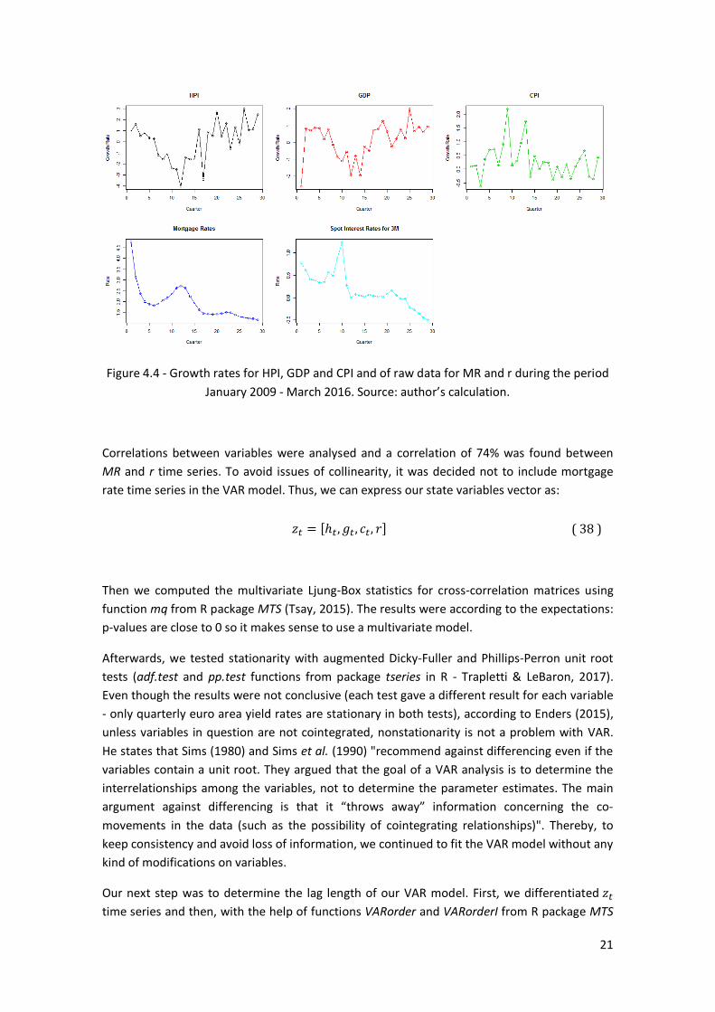
21

Figure 4.4 - Growth rates for HPI, GDP and CPI and of raw data for MR and r during the period January 2009 - March 2016. Source: author’s calculation.

Correlations between variables were analysed and a correlation of 74% was found between MR and r time series. To avoid issues of collinearity, it was decided not to include mortgage rate time series in the VAR model. Thus, we can express our state variables vector as:

𝑧𝑡 = [ℎ𝑡 ,𝑔𝑡 , 𝑐𝑡 , 𝑟] ( 38 )

Then we computed the multivariate Ljung-Box statistics for cross-correlation matrices using function mq from R package MTS (Tsay, 2015). The results were according to the expectations: p-values are close to 0 so it makes sense to use a multivariate model.

Afterwards, we tested stationarity with augmented Dicky-Fuller and Phillips-Perron unit root tests (adf.test and pp.test functions from package tseries in R - Trapletti & LeBaron, 2017). Even though the results were not conclusive (each test gave a different result for each variable - only quarterly euro area yield rates are stationary in both tests), according to Enders (2015), unless variables in question are not cointegrated, nonstationarity is not a problem with VAR. He states that Sims (1980) and Sims et al. (1990) "recommend against differencing even if the variables contain a unit root. They argued that the goal of a VAR analysis is to determine the interrelationships among the variables, not to determine the parameter estimates. The main argument against differencing is that it “throws away” information concerning the co-movements in the data (such as the possibility of cointegrating relationships)". Thereby, to keep consistency and avoid loss of information, we continued to fit the VAR model without any kind of modifications on variables.

Our next step was to determine the lag length of our VAR model. First, we differentiated 𝑧𝑡 time series and then, with the help of functions VARorder and VARorderI from R package MTS

22

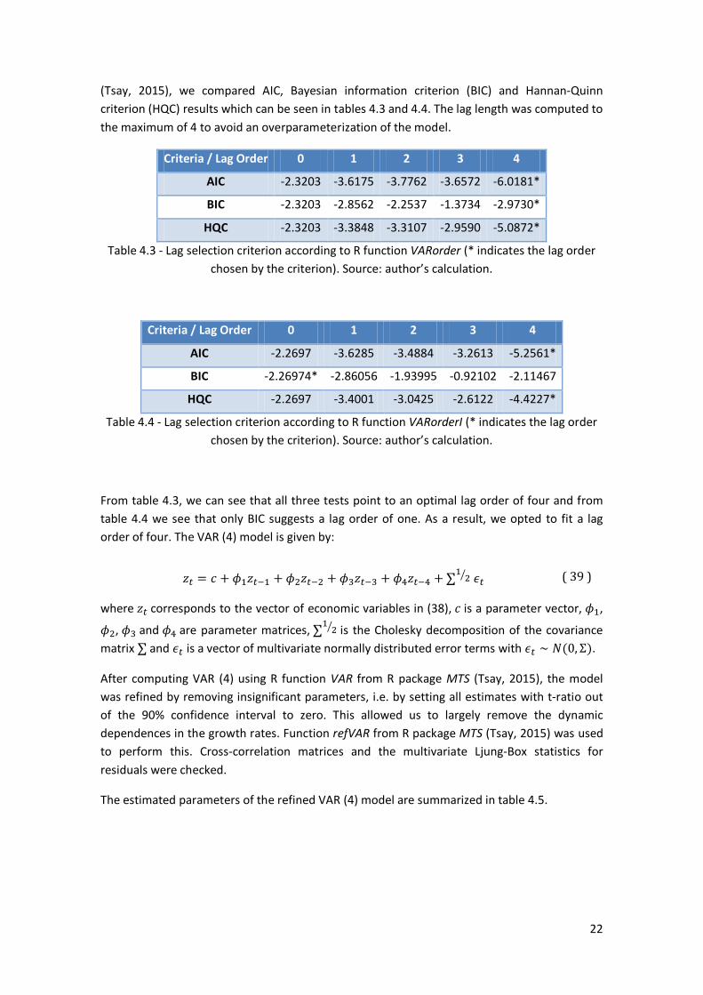
(Tsay, 2015), we compared AIC, Bayesian information criterion (BIC) and Hannan-Quinn criterion (HQC) results which can be seen in tables 4.3 and 4.4. The lag length was computed to the maximum of 4 to avoid an overparameterization of the model.

Criteria / Lag Order 0 1 2 3 4

AIC -2.3203 -3.6175 -3.7762 -3.6572 -6.0181*

BIC -2.3203 -2.8562 -2.2537 -1.3734 -2.9730*

HQC -2.3203 -3.3848 -3.3107 -2.9590 -5.0872*

Table 4.3 - Lag selection criterion according to R function VARorder (* indicates the lag order chosen by the criterion). Source: author’s calculation.

Criteria / Lag Order 0 1 2 3 4

AIC -2.2697 -3.6285 -3.4884 -3.2613 -5.2561*

BIC -2.26974* -2.86056 -1.93995 -0.92102 -2.11467

HQC -2.2697 -3.4001 -3.0425 -2.6122 -4.4227*

Table 4.4 - Lag selection criterion according to R function VARorderI (* indicates the lag order chosen by the criterion). Source: author’s calculation.

From table 4.3, we can see that all three tests point to an optimal lag order of four and from table 4.4 we see that only BIC suggests a lag order of one. As a result, we opted to fit a lag order of four. The VAR (4) model is given by:

𝑧𝑡 = 𝑐 + 𝜙1𝑧𝑡−1 + 𝜙2𝑧𝑡−2 + 𝜙3𝑧𝑡−3 + 𝜙4𝑧𝑡−4 + ∑1 2� 𝜖𝑡 ( 39 )

where 𝑧𝑡 corresponds to the vector of economic variables in (38), 𝑐 is a parameter vector, 𝜙1,

𝜙2, 𝜙3 and 𝜙4 are parameter matrices, ∑1 2� is the Cholesky decomposition of the covariance matrix ∑ and 𝜖𝑡 is a vector of multivariate normally distributed error terms with 𝜖𝑡 ∼ 𝑁(0,Σ).

After computing VAR (4) using R function VAR from R package MTS (Tsay, 2015), the model was refined by removing insignificant parameters, i.e. by setting all estimates with t-ratio out of the 90% confidence interval to zero. This allowed us to largely remove the dynamic dependences in the growth rates. Function refVAR from R package MTS (Tsay, 2015) was used to perform this. Cross-correlation matrices and the multivariate Ljung-Box statistics for residuals were checked.

The estimated parameters of the refined VAR (4) model are summarized in table 4.5.

23

VAR (4): 𝒛𝒕 = 𝒄 + 𝝓𝟏𝒛𝒕−𝟏 + 𝝓𝟐𝒛𝒕−𝟐 + 𝝓𝟑𝒛𝒕−𝟑 + 𝝓𝟒𝒛𝒕−𝟒 +∑𝟏 𝟐� 𝝐𝒕

𝒛𝒕 𝒄 (4x1) 𝝓𝟏 (4x4) 𝝓𝟐 (4x4)

𝒉𝒕 0.000 - 0.629 0.788 0.000 0.000 0.000 0.000 0.000 - 2.788

𝒈𝒕 0.000 0.000 - 0.381 - 1.283 0.000 - 0.444 0.000 - 0.387 0.000

𝒄𝒕 0.000 - 0.234 0.000 - 0.339 0.000 0.000 0.428 - 0.346 0.000

𝒓 0.000 0.000 0.000 0.261 0.000 0.000 0.000 0.000 0.000

𝝓𝟑 (4x4) 𝝓𝟒 (4x4)

0.000 0.000 0.000 0.000 0.000 0.000 0.000 0.000

0.000 0.476 - 1.320 1.055 0.000 - 0.343 - 0.942 - 2.449

0.000 0.000 0.000 0.000 0.000 0.000 0.288 0.000

0.000 0.000 0.000 0.000 0.046 0.000 0.000 - 0.458

𝚺 (4x4)

1.461 - 0.107 0.039 - 0.000

0.139 0.038 - 0.014

0.168 - 0.002

0.023

Table 4.5 - Estimated parameters of refined VAR (4) model (results rounded to 3 decimal places). Source: author’s calculation.

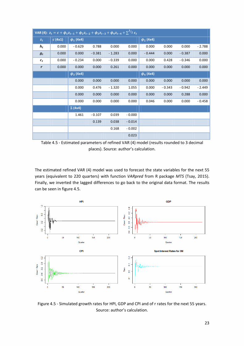
The estimated refined VAR (4) model was used to forecast the state variables for the next 55 years (equivalent to 220 quarters) with function VARpred from R package MTS (Tsay, 2015). Finally, we inverted the lagged differences to go back to the original data format. The results can be seen in figure 4.5.

Figure 4.5 - Simulated growth rates for HPI, GDP and CPI and of r rates for the next 55 years. Source: author’s calculation.

24

5. A REVERSE MORTGAGE SIMULATOR

Now that we have described a termination model and a VAR model for economic variables, we will use them to simulate the input variables of a reverse mortgage simulator so that we can determine the expected present value of lender's net payoff and the expected present value of the NNEG.

The house prices projections are computed based on 10,000 stochastic paths. These paths were simulated with function sde.sim from R package sde (Iacus, 2016) and with the logarithm of the lagged differences of the quarterly house price index from 2008 until 2016. The mortgage rate estimations were obtained from the previously described VAR (4) model and the prospective lifetables from the Lee-Carter's termination model, also earlier explained.

To decide the risk-based capital level for solvency requirement we consider VaR and CVaR risk measures at a 99% confidence level. We also include a sensitivity analysis to key model assumptions like borrower's age at the beginning of the contract, initial house price, mortality tables, borrowing ratio, loan to value ratio (LTV) and interest rate on the loan to better understand the impact of contract settings.

The following simulation results only address LS RM cases. The analysis of other typical contracts is left for further research.

5.1. BASELINE SCENARIO

In our baseline scenario, we consider a single male borrower aged 75 who lives in Portugal and with an initial house price of 120,000€10. To finance his expenses he decided to sign a RM contract. Assuming that the individual will not live beyond 125 years, the maximum contract duration considered is thus 50 years. It is also assumed that the average time delay from the point of contract exit until property's sale is 6 months. The lender's borrowing rate is set to 92% because 8% is the standard risk-based capital for mortgages under Basel II (Cho et al., 2013), and the remaining 8% are financed by lender's capital. Sale's transaction costs are set at 5% because this is the most usual commission rate used by real estate agencies in Portugal ("Quanto custa vender," 2013). LTV is set to 40% as in Cho et al. (2013). We assume a 1% fixed annual interest rate on the loan, in line with European interest rates at the time and this study was conducted assuming a continuously compounded house rental dividend yield of 0%.

Baseline scenario results are displayed on table 5.1, panel A. Figure 5.1 shows how the average house price and the RM accumulated loan balance develop throughout time. If we keep track on the slope of these two lines we can see that somewhere in time the accumulated loan balance will cross over the value of the property and that is the point where negative equity arises. Most of the time, negative equity events are triggered by house price volatility and even though this is unlikely to happen to LS RM contracts, it is a possibility in extreme scenarios of real estate market downturns.

10 According to section 2, the average useful area is 109 m2 and the average value from bank evaluation of living quarters in Portugal is 1,111€/m2, as reported by Statistics Portugal.

25

Figure 5.1 - Average house price and average loan balance for LS RM in the baseline scenario. Source: author’s calculation.

Figure 5.2 illustrates the expected financing cost for a LS RM contract. As time goes by, these costs increase in the same way the accumulated loan balance increases, which means the lender will incur in a loss when the total financing cost of the loan exceeds the property sale proceeds.

Figure 5.2 - Average financing cost for LS RM in the baseline scenario. Source: author’s calculation.

Panel A from table 5.1 shows that lender's expected net payoff is positive and higher than the LS payment. VaR and CVaR with a 99% level of confidence confirm that the lender does not face financial risks, as we can also observe in figure 5.3.

Figure 5.3 - Expected average of present value of the lender's net payoff for LS RM in the baseline scenario. Source: author’s calculation.

26

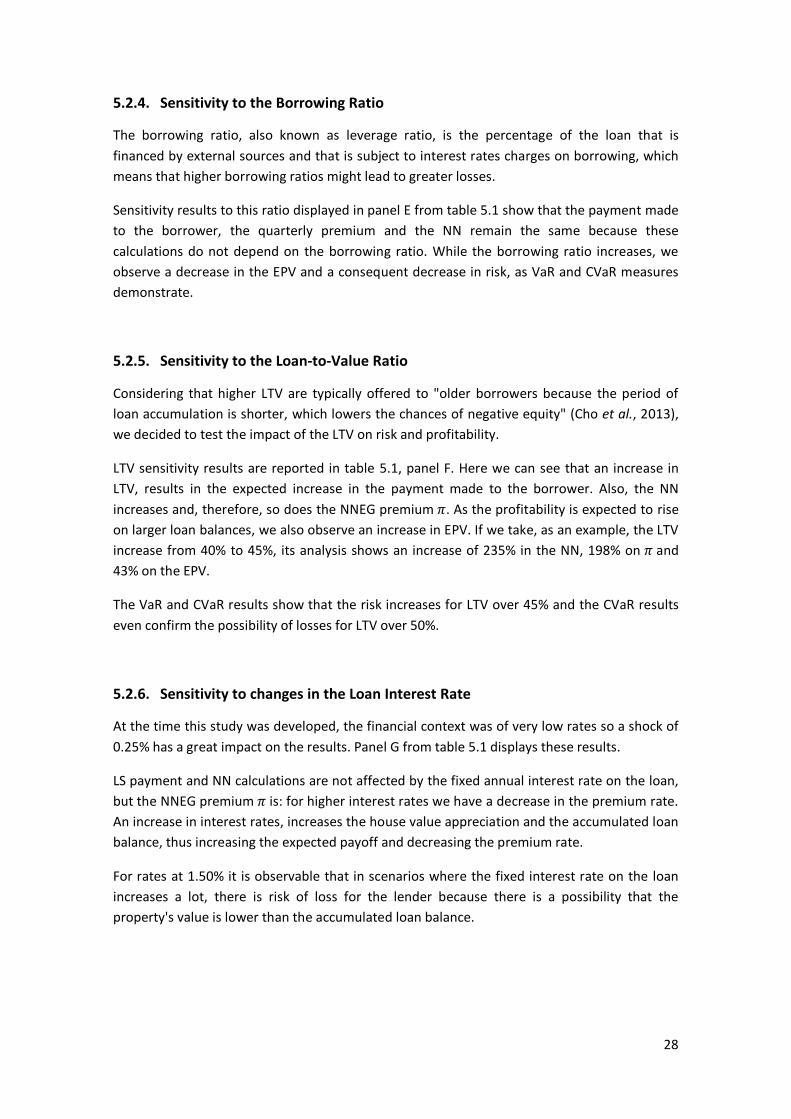
Payment NN 𝝅 EPV VaR CVaR

A. Baseline - 𝐀𝐠𝐞 = 𝟕𝟓 𝐲𝐞𝐚𝐫𝐬, 𝐇𝟎 = 𝟏𝟐𝟎,𝟎𝟎𝟎€, 𝐌𝐈 = 𝟏𝟎𝟎%, 𝛗 = 𝟗𝟐%, 𝐋𝐓𝐕 = 𝟒𝟎%, 𝐫𝐭𝐤 = 𝟏.𝟎𝟎%

48,000€ 248€ 0.041% 50,495€ 38,177€ 36,675€

B. Sensitivity analysis - initial borrower's age

Age 65 48,000€ 589€ 0.054% 63,068€ 49,218€ 11,303€

70 48,000€ 394€ 0.048% 57,630€ 43,815€ 33,682€

80 48,000€ 144€ 0.034% 42,317€ 32,400€ 32,400€

85 48,000€ 75€ 0.027% 33,700€ 26,631€ 26,631€

C. Sensitivity analysis - initial house price (𝐇𝟎)

𝑯𝟎 40,000€ 16,000€ 83€ 0.041% 16,832€ 12,726€ 12,225€

80,000€ 32,000€ 165€ 0.041% 33,663€ 25,451€ 24,450€

160,000€ 64,000€ 330€ 0.041% 67,326€ 50,903€ 48,900€

200,000€ 80,000€ 413€ 0.041% 84,158€ 63,628€ 61,125€

D. Sensitivity analysis - mortality improvements (MI)

MI 90% 48,000€ 247€ 0.038% 49,269€ 37,817€ 35,974€

95% 48,000€ 248€ 0.040% 49,895€ 38,005€ 36,335€

105% 48,000€ 248€ 0.042% 51,072€ 38,335€ 36,965€

110% 48,000€ 248€ 0.043% 51,629€ 38,480€ 37,213€

E. Sensitivity analysis - borrowing ratio (𝛗)

𝝋 87.0% 48,000€ 248€ 0.041% 74,355€ 62,038€ 60,536€

89.5% 48,000€ 248€ 0.041% 62,425€ 50,107€ 48,605€

94.5% 48,000€ 248€ 0.041% 38,564€ 26,247€ 24,745€

97.0% 48,000€ 248€ 0.041% 26,634€ 14,316€ 12,814€

F. Sensitivity analysis - loan to value ratio (LTV)

LTV 30% 36,000€ 9€ 0.002% 29,337€ 28,633€ 28,633€

35% 42,000€ 57€ 0.011% 37,076€ 33,405€ 33,405€

45% 54,000€ 833€ 0.122% 72,106€ 42,949€ 21,749€

50% 60,000€ 2,311€ 0.305% 99,630€ 39,762€ -76,714€

G. Sensitivity analysis - fixed annual interest rate on the loan (𝐫𝐭𝐤)

𝒓𝒕𝒌 0.50% 48,000€ 248€ 0.043% 39,117€ 20,749€ 20,749€

0.75% 48,000€ 248€ 0.042% 45,634€ 29,840€ 29,840€

1.25% 48,000€ 248€ 0.040% 53,008€ 45,829€ 33,335€

1.50% 48,000€ 248€ 0.039% 51,806€ 2,165€ -40,036€

Table 5.1 - Risk and profitability measures for LS RM payments in the baseline and sensitivity scenarios. Source: author’s calculation.

27

Table 5.1 displays baseline and sensitivity scenarios results. NN represents the expected present value of the NNEG, 𝜋 the annual insurance premium for the NNEG and EPV is the expected present value of the lender's net payoff. VaR represents the Value-at-Risk and CVaR the corresponding Conditional Value-at-Risk of the EPV calculated at a 99% confidence level.

5.2. SENSITIVITY ANALYSIS

5.2.1. Sensitivity to the Initial Age

Test results to the initial borrower's age are provided in panel B from table 5.1. Here we can see that the payment does not change and that the NN and the NNEG premium 𝜋 decrease along with the age increase. This happens because as the age increases, the expected loan duration, i.e., the life expectancy, decreases so the risk of crossover is lower.

EPV develops on the same direction as NN and as the NNEG premium 𝜋: for later ages, the EPV is lower. For example, when the initial borrower's age goes from 75 to 80, results show that the EPV decreases 16%. For lower contract durations there is less time for the property value to appreciate which results in less profits to the lender and, consequently, in a decrease of the net payoff while age is raised.

5.2.2. Sensitivity to the Initial House Price

Panel C from table 5.1 showcases the sensitivity results to the initial house price, which is the value of the property at the moment the contract of RM is signed. We can conclude from them that as the initial house price increases the payment made to the borrower also increases in absolute terms, and EPV also increases. However, the NNEG premium 𝜋 does not change because its calculation does not depend on the house price. VaR and CVaR results express a risk decrease.

5.2.3. Sensitivity to Mortality Improvements

Mortality rates are the major contributor for RM contract's termination and lower mortality rates imply an extension of contract's duration and, therefore, in higher accumulated loan balances.

Longevity risk results are reported in panel D of table 5.1. There we can see that the risk of non-negative events increases, but at a slow pace. The NNEG premium 𝜋 also evidences low increases because the payments are spread over the whole contract's duration. High mortality rates also result in higher EPV because the lending margin has less time to accumulate even though the property's value does not have it to appreciate.

VaR and CVaR measures show that there is no risk of loss in none of the presented scenarios.

28

5.2.4. Sensitivity to the Borrowing Ratio

The borrowing ratio, also known as leverage ratio, is the percentage of the loan that is financed by external sources and that is subject to interest rates charges on borrowing, which means that higher borrowing ratios might lead to greater losses.

Sensitivity results to this ratio displayed in panel E from table 5.1 show that the payment made to the borrower, the quarterly premium and the NN remain the same because these calculations do not depend on the borrowing ratio. While the borrowing ratio increases, we observe a decrease in the EPV and a consequent decrease in risk, as VaR and CVaR measures demonstrate.

5.2.5. Sensitivity to the Loan-to-Value Ratio

Considering that higher LTV are typically offered to "older borrowers because the period of loan accumulation is shorter, which lowers the chances of negative equity" (Cho et al., 2013), we decided to test the impact of the LTV on risk and profitability.

LTV sensitivity results are reported in table 5.1, panel F. Here we can see that an increase in LTV, results in the expected increase in the payment made to the borrower. Also, the NN increases and, therefore, so does the NNEG premium 𝜋. As the profitability is expected to rise on larger loan balances, we also observe an increase in EPV. If we take, as an example, the LTV increase from 40% to 45%, its analysis shows an increase of 235% in the NN, 198% on 𝜋 and 43% on the EPV.

The VaR and CVaR results show that the risk increases for LTV over 45% and the CVaR results even confirm the possibility of losses for LTV over 50%.

5.2.6. Sensitivity to changes in the Loan Interest Rate

At the time this study was developed, the financial context was of very low rates so a shock of 0.25% has a great impact on the results. Panel G from table 5.1 displays these results.

LS payment and NN calculations are not affected by the fixed annual interest rate on the loan, but the NNEG premium 𝜋 is: for higher interest rates we have a decrease in the premium rate. An increase in interest rates, increases the house value appreciation and the accumulated loan balance, thus increasing the expected payoff and decreasing the premium rate.

For rates at 1.50% it is observable that in scenarios where the fixed interest rate on the loan increases a lot, there is risk of loss for the lender because there is a possibility that the property's value is lower than the accumulated loan balance.

29

6. CONCLUSIONS

In this study we analyse the profitability and the risk of LS RM loans from provider's perspective. The pricing framework for simulation incorporates a Lee-Carter's stochastic mortality model to derive expected longevity improvements of the Portuguese population and a VAR model to forecast economic variables.

We find that borrower's age at the beginning of the contract, as well as the mortality improvements, play a very important role on product's profitability and riskiness. Sensitivity results show that for younger borrowers the profits are higher and there is no risk of losses for the lender. On the other hand, higher longevity rates allow property's value to appreciate but also imply higher financing costs for the lender. Higher LTV represent higher earnings but also imply more risk to lenders. Sensitivity results to loan interest rate changes were produced in a financial context of low interest rates, so the model is very sensitive to shocks on this variable, as mortgages rates and house appreciation do not change by the same amount. Lower borrowing ratios offer higher profits and more valuable properties also bring more earnings to the RM providers without being so exposed to risk.

From the lender's perspective, in all tested scenarios, LS RM contracts are expected to be profitable. Providers would only incur in loss in extreme scenarios, like in a real estate market collapse. However, lenders should always hold capital to face this risk.

Our results and literature review evidence the importance of providing these kind of financial products to ageing populations, like the Portuguese one. Both homeowners and investors would take advantages from this if the market started to develop more quickly. It is important to highlight that a good financial literacy of the consumers is a key factor for its commercialization. Governments should also regulate this market for a smooth implementation of the product.

A future line of work could be the understanding of the impact of borrower's age, gender, marital status, wealth and home address in the contract's termination. As mentioned before, the risk of termination can also be triggered by borrower's mobility which can also be discussed in future studies.

Concerning the models used, it would be interesting to discount the cash flows arising from the NNEG by using risk-adjusted stochastic discount factors like in Cho et al. (2013).

Regarding risk and profitability analysis, future studies can focus on doing it to fixed income streams and inflation-indexed income streams payments and compare these results with the here studied lump sums and with other similar equity release products.

As a final note, the R scripts will be supplied upon request.

30

7. BIBLIOGRAPHY

Abraham, J., & Hendershott, P. (1994). Bubbles in Metropolitan Housing Markets. Journal of Housing Research 7(2), pp. 191–208.

Alai, D. H., Chen, H., Cho, D., Hanewald, K. & Sherris, M. (2013). Developing Equity Release Markets: Risk Analysis for Reverse Mortgages and Home Reversions. UNSW Australian School of Business Research Paper No. 2013ACTL01.

Alexandre, F., Aguiar-Conraria, L., Bação, P. & Portela, M. (2011). A Poupança em Portugal. APS - Associação Portuguesa de Seguradores, p. 9.

Bank of Portugal: http://www.bportugal.pt/en-US

Booth, H., Maindonald, J., & Smith, L. (2002). Applying Lee-Carter under conditions of variable mortality decline. Population Studies, 56 (3), pp. 325–336.

Booth, H. & Tickle, L. (2003). The future aged: new projections of Australia’s elderly population. Population Studies, 22 (4), pp. 38–44.

Booth, H. & Tickle, L. (2008). Mortality Modeling and Forecasting: A review of methods. ADSRI Working Paper No. 3.

Bourgeois-Pichat, J. (1952). Essai sur la mortalité biologique de l’homme. Population, 7(3), pp. 1–31.

Bravo, J. M. (2008). Construção de Tábuas de Mortalidade Contemporâneas e Prospectivas: Aplicações Actuariais e Cobertura do Risco de Longevidade. Ph.D. thesis, Universidade de Évora, Portugal.

Bravo, J. M. (2010). Lee-Carter mortality projection with "Limit Life Table". In EUROSTAT - European Commission (eds.), Work session on demographic projections, EUROSTAT-EC Collection: Methodologies and working papers, Theme: Population and Social Conditions, pp. 231–240.

Bravo, J. M. (2012). Sistemas de Segurança Social em Portugal: arquitectura de um novo modelo social e contributos para o debate sobre a reforma do regime de pensões. APFIPP, Dezembro.

Bravo, J. M. (2017). Contratos intergeracionais e consistência temporal na gestão da protecção social: Implicações Políticas e Reforma do Sistema de Pensões. in "Envelhecimento na Sociedade Portuguesa: Pensões, Família e Cuidados", Imprensa de Ciências Sociais, Universidade de Lisboa, pp. 61–96.

Bravo, J. M., Afonso, L. & Guerreiro, G. (2013). Avaliação Actuarial do Regime de Pensões da Caixa Geral de Aposentações: formulação actual e impacto das medidas legislativas.

31

Bravo, J. M., Afonso, L. & Guerreiro, G. (2014). Avaliação Actuarial do Sistema Previdencial da Segurança Social e Prestação Única da Segurança Social. GEP, MSESS, Lisboa, Dezembro.

Bravo, J. M., Coelho, E. & Magalhães, M. G. (2010). Mortality projections in Portugal. In EUROSTAT - European Commission (eds.), Work session on demographic projections, EUROSTAT-EC Collection: Methodologies and working papers, Theme: Population and Social Conditions, pp. 241–252.

Bravo, J. M. & Silva, C. P. da (2012). Prospective Lifetables: Life Insurance Pricing and Hedging in a Stochastic Mortality Environment. CEFAGE-UE Working Paper 2012/01.

Brouhns, N., Denuit, M., & Vermunt, J. (2002). A Poisson log-bilinear regression approach to the construction of projected lifetables. Insurance: Mathematics & Economics, 31 (3), pp. 373–393.

Canadian Home Income Reverser Mortgage Plan: https://www.chip.ca

Carter, L. & Prkawetz, A. (2001). Examining Structural Shifts in Mortality using the Lee-Carter Method. MPIDR WP 2001-007, Center for Demography and Ecology Information, University of Wisconsin-Madison.

Chen, H., Cox, S. H., & Wang, S. S. (2010). Is the Home Equity Conversion Mortgage in the United States Sustainable? Evidence from Pricing Mortgage Insurance Premiums and Non-Recourse Provisions Using Conditional Esscher Transform. Insurance: Mathematics and Economics, 46 (2), pp. 371–384.

Chinloy, P. & Megbolugbe, I. F. (1994). Reverse Mortgages: Contracting and Crossover Risk. Real Estate Economics, 22(2), pp. 367–386.

Cho, D., Hanewald, K. & Sherris, M. (2013). Risk Management and Payout Design of Reverse Mortgages. UNSW Australian School of Business Research Paper No. 2013ACTL0.

Davidoff, T. & Welke, G. (2007). Selection and Moral Hazard in the Reverse Mortgage Market. Available at http://strategy.sauder.ubc.ca/davidoff/RMsubmit3.pdf

Debón Aucejo, AM., Montes, F. & Sala, R. (2013). Pricing Reverse Mortgages in Spain. European Actuarial Journal, 3, pp. 23–43.

Debón, A., Montes, F., & Puig, F. (2008). Modeling and Forecasting Mortality in Spain. European Journal of Operation Research, 189 (3), pp. 624–637.

Denuit, M. & Goderniaux, A. (2005). Closing and Projecting Lifetables using Log-linear Models. Bulletin del’Association Suisse des Actuaries, 1, pp. 29–49.

Dinheiro Vivo - Mercado Imobiliário: Quanto custa vender a minha casa (24/06/2013). Available at: https://www.dinheirovivo.pt/carreiras/quanto-custa-vender-a-minha- casa/

32

Enders, W. (2015). Applied Econometric Time Series (4rd edition). New York: John Wiley & Sons. Chapter 5, pp. 290–291.

European Central Bank: https://www.ecb.europa.eu/stats/money/yc/html/index.en.html

European Commission (2015). The 2015 Ageing Report Economic and budgetary projections for the 28 EU Member States (2013-2060). EUROPEAN ECONOMY, 3/2015.

European Commission (DG EMPL) and Social Protection Committee (SPC WG-AGE) (2015). The 2015 Pension Adequacy Report: current and future income adequacy in old age in the EU. Volume I. Luxembourg: Publications Office of the European Union, pp. 49-84 and 333–354.

Goodman, L. (1979). Simple models for the analysis of association in cross classifications having ordered categories. Journal of the American Statistical Association, 74, pp. 537– 552.

Guillen, M. & Vidiella-i-Anguera, A. (2005). Forecasting Spanish natural life expectancy. Risk Analysis, 25 (5), pp. 1161–1170.

Herranz González, R. (2006). Hipoteca Inversa y figuras afines. Madrid: Portal Mayores. Informes Portal Mayores, 49.

Hyndman, R. J. (2016). Package ‘forecast’: Forecasting Functions for Time Series and Linear Models. R package version 7.1. Available at: https://cran.r-project.org/web/packages/forecast/forecast.pdf

Hosty, G. M., Groves, S. J., Murray, C. A., & Shah, M. (2008). Pricing and Risk Capital in the Equity Release Market. British Actuarial Journal, 14 (1), pp. 41–91.

Institute of Actuaries (2005). Equity release report 2005. Volume 2: Technical supplement: pricing considerations. Available at http://www.actuaries.org.uk/research-and-resources/documents/equity-release- report-2005-volume-2-technical-supplement-pricing-co.

Iacus, S. M. (2016). Package ‘sde: Simulation and Inference for Stochastic Differential Equations. R package version 2.0.15. Available at: https://cran.r-project.org/web/packages/sde/sde.pdf

Inquérito à Situação Financeira das Famílias (2010). Available at: https://www.bportugal.pt/pt- PT/EstudosEconomicos/Publicacoes/ISFFamilias/Publicacoes/isff_2010_p.pdf

Ji, M. (2011). A Semi-Markov Multiple State Model for Reverse Mortgage Terminations. University of Waterloo.

Lee, R. (2000). The Lee-Carter Method for Forecasting Mortality, with various extensions and applications. North American Actuarial Journal, 4(1), pp. 80–91.

Lee, R. & Carter, L. (1992). Modeling and Forecasting U.S. mortality. Journal of the American Statistical Association, 87 (419), pp. 659–671.

33

Lee, R. & Miller, D. (2001). Evaluating the Performance of the Lee-Carter Method for Forecasting Mortality. Demography, 38 (4),pp. 537–549.

Lee, R. & Nault, F. (1993). Modeling and forecasting provincial mortality in Canada. Montreal. World Congress of the International Union for Scientific Study of Population.

Lee, R. & Rofman, R. (1994). Modelación y proyección de la mortalidad en Chile. Notas Población, 22 (59), pp. 182–213.

Li, J.S.-H., Hardy, M.R. & Tan, K.S. (2010). On Pricing and Hedging the No-Negative-Equity- Guarantee in Equity Release Mechanisms. Journal of Risk and Insurance, 77, pp. 499– 522.

Martins, T. M. C. (2011). Reverse Mortgage em Portugal: uma opção viável?. ISCTE Business School, Instituto Universitário de Lisboa.

Miceli, T. J. & Sirmans, C. F. (1994). Reverse Mortgages and Borrower Maintenance Risk. Journal of the American Real Estate and Urban Economics Association, 22 (2), pp. 433 - 450.

Muellbauer, J., & Murphy, A. (1997). Booms and Busts in the UK Housing Market. The Economic Journal 107 (445), pp. 1701-1727.

PORDATA - Database of Contemporary Portugal: http://www.pordata.pt/en

Reifner, U., Clerc-Renaud, S., Pérez-Carrillo, E. F., Tiffe, A. & Knobloch, M. (2007). Study on Equity Release Schemes in the EU - Part I: General Report. Institut für Finanzdienstleistungen e.V., page I.

"Reforma das pensões: há soluções técnicas, não há solução política" by Corrêa de Aguiar, Margarida (2015). Observador. Available at: http://observador.pt/opiniao/reforma- das-pensoes-ha-solucoes-tecnicas-nao-ha-solucao-politica/

Renshaw, A. & Haberman, S. (2003). Lee-Carter mortality forecasting: a parallel generalized linear modeling approach for England and Wales mortality projections. Journal of the Royal Statistical Society C, 52 (1), pp. 119–137.

Rocha, R., Vittas, D. & Rudolph, Heinz P. (2011). Annuities and Other Retirement Products - Designing the Payout Phase. The World Bank, 1st edition, Washington, D.C.

Senior Australians Equity Release Association of Lenders: http://www.sequal.com.au

Shao, A. W., Hanewald, K. & Sherris, M. (2014). Reverse Mortgage Pricing and Risk Analysis Allowing for Idiosyncratic House Price Risk and Longevity Risk. UNSW Australian School of Business Research Paper No. 2014ACTL01.

Sherris, M. & Sun, D. (2010). Risk Based Capital and Pricing for Reverse Mortgages Revisited. UNSW Australian School of Business Research Paper No. 2010ACTL04.

34

Shiller, R. J. & Weiss, A. N. (2000). Moral Hazard in Home Equity Conversion. Real Estate Economics, 28(1), pp. 1–31.

Sims, Christopher (1980). Macroeconomics and Reality. Econometrica, 48, pp. 1–49

Sims, C., Stock, J. & Watson, M. W. (1990). Inference in Linear Time Series Models with Some Unit Roots. Econometrica, 58, pp. 113–44.

Statistics Portugal: http://www.ine.pt

The Human Mortality Database: http://www.mortality.org/

Trapletti, A., Hornik, K. & LeBaron, B. (2017). Package ‘tseries’: Time Series Analysis and Computational Finance. Rpackage version 0.10-42. Available at: https://cran.r- project.org/web/packages/tseries/tseries.pdf

Tsay, R. S. (2015). Package ‘MTS’: All-Purpose Toolkit for Analyzing Multivariate Time Series (MTS) and Estimating Multivariate Volatility Models. Rpackage version 0.33. Available at: https://cran.r-project.org/web/packages/MTS/MTS.pdf

Vaz, B. R. (2014). Reverse Mortgage em Portugal: Uma abordagem actuarial. Faculdade de Ciências e Tecnologia da Universidade Nova de Lisboa. Available at: https://run.unl.pt/handle/10362/14138

Wilmoth, J. (1996). Mortality projections for Japan: A comparison of four methods. In: Graziella Caselli and Alan Lopez (eds.), Health and Mortality among Elderly Populations, Oxford University Press, pp. 266-287.

Federal Housing Administration - Home Equity Conversion Mortgage: http://portal.hud.gov/hudportal/HUD?src=/program_offices/housing/sfh/hecm/hecm home