Valuation of Real Options with Flexible Early Exercise in ... · Valuation of Real Options with...

1

Valuation of Real Options with Flexible Early Exercise in a

Competitive Environment:

The Case of Performance Improvement Packages

Cedric Y. Justin1 and Dimitri N. Mavris

2

Georgia Institute of Technology, Atlanta, Georgia

Commercial aircraft developments are major endeavors which strain significantly the resources

of original equipment manufacturers. These developments represent huge bets for the companies

undertaking them due to the assumptions made when business plans are laid out and the abundance of

uncertainties both at the technical and market levels. The long development cycles and the long lives

of the aircraft once in operations force aircraft manufacturers to speculate regarding future airline

needs and future states of the world. One possibility to mitigate these risks is through a continuous

optimization of the airframe and its engines after it has entered service. These continuous

developments help manufacturers stretch the operating lives of their designs by keeping them up-to-

date and therefore relevant in a competitive environment. Performance improvement packages (PIP)

represent a means for aircraft and engine manufacturers to offer airlines the ability to infuse new

technologies into existing assets at a minimum capital expenditure. Standard capital budgeting

methods are not well suited to assess the economic performance of programs subject to significant

uncertainty because they fail to account for the flexibility offered to management to steer programs

into profitable directions. Similarly, these methods do not usually capture the dynamic nature of

markets and the erosion of leadership positions over time. The on-going research tries to overcome

some of these challenges by proposing a real-option based method to help substantiate development

strategies in the aerospace industry. A new method is proposed to evaluate real-options featuring early

exercise possibilities by cross-fertilizing techniques used in the finance industry, in statistics, and in

actuarial sciences. It is articulated around the use of an Esscher transform and its non-parametric

empirical approximation to perform a risk neutralization, a bootstrapping technique to resample the

evolution of the underlying development program value, and finally a regression-based technique to

value real-options with early-exercise possibilities. The proposed method is applied to the evaluation

of a performance improvement package for a commercial aircraft.

Keywords: Real-options, Simulation, Esscher Transform, Resampling, Bootstrapping, Early Exercise

1 Introduction

Aircraft development cycles are both long and expensive and their lengths force manufacturers to speculate

regarding future airline needs and future states of the world. Tremendous risks are associated with these

developments and manufacturers are reluctant to develop new airliners from scratch. On the other side of the market,

airlines buy aircraft with operating lives exceeding twenty years, and renewing the fleet is a major decision that may

affect their global competitiveness for over a decade. Facing unprecedented fuel expenses, airlines pressure aircraft

1 PhD Candidate, e-mail: [email protected] 2 Boeing Professor of Advanced Aerospace Systems, e-mail: [email protected]

2

manufacturers to produce significantly more efficient designs. The airline fleet selection process is a complex task

relying on multi-attribute analyses. According to Paul Clark [1], there are key buying criteria in the decision and

these vary slightly from customer to customer. However, these key factors revolve around the economic, the

performance, the comfort and the environmental aspects, with the economic and performance aspects accounting for

about seventy percent of the decision.

One venue for manufacturers to mitigate these risks is through the continuous optimization and

improvement of their product-portfolio even after entry into service. These developments help manufacturers stretch

the operating lives of their aircraft designs by keeping them up-to-date and therefore relevant in a competitive

environment. Performance Improvement Packages (PIP) present a way for aircraft manufacturers to offer airlines the

ability to infuse new technologies into existing assets [2] and to rejuvenate their fleet at a minimum capital

expenditure. These packages have been widely used in the aircraft and engine manufacturing industry and have

often been proposed to operators as stop-gap measures to improve the economics of aircraft currently on the market.

For instance, McDonnell Douglas introduced a series of PIP [3] in the 1990’s to improve the aerodynamics, reduce

the drag, and improve the fuel-burn of its flagship MD-11 aircraft as the aircraft was not meeting promised

specifications at entry in service. CFM International announced in 2007 the first delivery of a Tech Insertion

package and in 2011 announced the availability of a new performance improvement package for the CFM56-5B3

[4] turbofan engine. These aimed at reducing NOx emissions, improving fuel burn, and extending the time on-wing

of the engine. Another example is Boeing which introduced in 2009 refinements to the B777 aircraft that airlines

could purchase to increase range and payload [5]. These improvements involved reshaping tiny vortex generators on

the upper surface of the wing, optimizing the ram air intake system to reduce drag and drooping ailerons by two

degrees while in flight. Finally, in 2013 Airbus launched a Sharklet retrofit [6] for in-service aircraft of the A320

family. This retrofit brings new advanced wingtip devices to reduce fuel-burn by up to four percent and

consequently to reduce carbon emissions.

Still, developing, certifying, testing, and producing a performance improvement package is expensive and

manufacturers have to commit scarce engineering resources in return for hypothetical profits. To assess their

economic viability, manufacturer estimate development costs and forecast future demand by making assumptions

regarding the future state of the airline industry and the future state of the competition. Traditionally, discounted

cash flow analysis is used next to assess the economic performance of investments as reported by Graham and

Harvey [7]. This is however not well suited for projects involving significant upfront investments such as

development programs in the aerospace industry: indeed, with initial investments in the billions and aircraft

deliveries starting only several years later, the discounted cash flow analysis over-emphasizes initial cash-outflows

and undervalues streams of cash-inflows coming only years later. This leads to an undervaluation of many

development programs and possibly the rejection of potentially profitable development programs. Yet, new aircraft

developments are undertaken every year.

Part of this problem lays in the fact that discounted cash flow analyses are deterministic and therefore do

not handle well projects spanning over multiple years, featuring several decision tollgates and riddled with

uncertainties. One method to assess project viability under uncertainty uses real-options [8]. Real-options analysis is

an emerging field in corporate finance [9] where it is used to substantiate capital budgeting decisions. It is derived

from the financial options analysis pioneered with the seminal work of Black, Scholes [10] and Merton [11]. Real-

options analysis may be interpreted as an extension of the discounted cash flow analysis in that it uses the concept of

time-value of money but goes beyond and recognizes the fact that managers react to changes in the business

environment and actively steer projects into profitable directions. Consequently, a real-options approach accounts

for the flexibility offered to management to abandon unprofitable programs. This is particularly well suited for

aerospace development programs which usually feature critical tollgate reviews at which programs may be

abandoned. In the case of new aircraft developments, the major drivers affecting the profitability of a development

3

program include the growth of air transportation, the retirement of older less-efficient aircraft, as well as the

evolution of the energy prices (jet-fuel).

There is little doubt that real-options inspired methodologies present an attractive concept for capital

allocation budgeting problems due to their abilities to better mimic the decision processes that take place within

companies as uncertainty unfolds. However, as much as option-thinking seems promising for analyzing investments

featuring flexibility, the implementation and the adoption of real-options within companies has been slow[12]. There

may be several reasons to this and one of them may be the complexity of developing a relevant real-options

framework. While simpler models using the closed-form Black-Scholes formula have been attractive initially due to

their simplicity, their validity for corporate investment valuation may be questionable. Some of the assumptions

underpinning the Black-Scholes model are quite strong and may not be appropriate for corporate investments. More

generic methods using Monte Carlo simulations have been proposed over the years and relax some of these

assumptions but the explicit formulation of a model for the evolution of the business prospect value remains

problematic. Indeed, analysts typically have access to a lot of real data and may be able to model the evolution of

one or several source of uncertainty over time. Nevertheless, when several sources of uncertainty impact a

development program, fitting a model to simulate the stochastic evolution of the development program value

becomes significantly harder.

In this context, the current research proposes a new transparent and integrated methodology aimed at

investigating the viability of a strategic investment in a competitive environment. The value-driven methodology

will be the foundation for a strategic decision-making framework that facilitates the formulation of robust and

competitive solutions. The methodology is applied to the development of a performance improvement package for

an aircraft no longer in production. The package includes the addition of advanced wingtip devices to reduce drag

and therefore decrease fuel-burn, as well as some refinements to the engine to improve efficiency and further reduce

fuel-burn and emissions. The manufacturer has identified a gap in its development stream which makes it possible to

develop, certify, and produce the package. As a result, there are three reasons motivating this development: demand

by airlines for more efficient aircraft to reduce their exposure to fluctuating energy prices; extension of the operating

life of their fleet by making the aircraft more competitive with other offerings from the competition; and

identification of a gap in the development stream of the aircraft manufacturer that needs to be filled to keep

workforce busy. Decision makers have to identify whether the market conditions are currently optimal for the

commercial launch of this product and whether it makes sense to commit resources to this development. If not, the

manufacturer can delay the development and wait for trigger events that will ensure a successful development.

2 Development of the Performance Improvement Package

The performance improvement package consists of two subsets of technologies that can be retrofitted to a

family of aircraft currently in operations. The first subset consists in an advanced winglet device to be fitted at the

wingtip of the aircraft to reduce lift induced-drag. However, some structural strengthening of the wing spar is

required to fit the new winglet in order to cope with the increased wing bending moment. The second subset consists

in new materials and an advanced shaping of the fan blades for the engine as well as new alloys in the turbine

section. This results in increased fuel efficiency for the engine with lower specific fuel consumption as well as fewer

maintenance events. The performance improvement packages can be installed by airlines on their aircraft during

regular scheduled maintenance in their own facilities. The resulting impacts on several key metrics are quantified in

Table 1.

4

Table 1: Performance Improvement Package Impact on Key Metrics

SFC Induced Drag Vehicle Weight Maintenance Cost

Advanced Winglet -5.0% +0.5%

Updated Turbofan -1.0% -0.5% -1.0%

2.1 Development timeline

The development process for the Performance Improvement Package may be described as a staggered

development program featuring decision tollgates. It is articulated around four main phases, starting with the initial

market research and conceptual design, followed by preliminary and detailed developments, followed by

certification and testing, and finally ending with production. Each of these phases is separated by a decision tollgate

at which point management can exercise some flexibility and decide whether to pursue, delay, or abandon the

development altogether if the market conditions are not right. This development timeline is shown in Figure 1.

Figure 1: Development timeline and associated milestones

If the development program goes ahead, additional funding is committed and spent during the following

phase. All four of these phases do not have the same resource requirements: detailed development as well as

certification and testing to a lesser extent are the most expensive phases of the development program. Therefore, it is

unlikely that the program will be abandoned at the third or fourth decision tollgate given that the following phases

are relatively cheap and that so much has already been spent during the previous phases. Delaying or abandoning the

development is nevertheless a possibility at the first and second decision tollgates if conditions are not favorable.

2.2 Windows of possibilities

In this pilot study, the manufacturer has identified a gap in its development stream between two periods of

high activity. The first period of high activity is related to a previous development requiring substantial engineering

resources to complete the detailed design and to get certification. The second period of high activity concerns a

future development for the replacement of a current aircraft design that is getting obsolete. This second program is

therefore deemed vital for the profitability of the manufacturer and is projected to tie the engineering resources for

several years onwards. In between, there is a development gap during which the manufacturer has currently no

projected development and during which engineering resources might be available. This is an unfortunate situation

for aircraft and engine manufacturers as they have to retain the workforce to keep skilled and experienced engineers

in-house for future programs. In this context, a window of possibility for the development of the PIP program is

defined as the ability to undertake a development program. This situation is depicted in Figure 2.

Figure 2: Timeline of manufacturer development stream

2.3 Windows of opportunities

Of interest however are not windows of possibilities but rather windows of opportunities which are defined

as the timeframe during which, and the condition for which, launching a new development program is best. If

TimeInitial Market

Research

Detailed

DevelopmentCertification & Testing Production

Decision Tollgate 1 Decision Tollgate 2 Decision Tollgate 3 Decision Tollgate 4

$ $$ $$ $

PIP Development Timeline

TimeInitial R&D GapDevelopment Resources

Tied for Other Programs

Development Resources Projected to be

Tied for Other High Priority Programs

Manufacturer Development Stream:

Possibility window

5

decision-makers invest too early within the window of possibility, they only have limited information and this may

be risky as the future realization of uncertainty might undermine the development program. If decision makers

invest too late, risk also increases since the target market size is reduced as airlines ground older aircraft and airlines

become reluctant to invest in retrofits for an ageing fleet. To be meaningful to decision-makers, a window of

opportunity has to be contained within a window of possibility. Therefore, the largest window of opportunity is the

window of possibility.

In addition, windows of opportunities are not static: they morph in real time to adjust to the new reality that

unfolds. Increasing energy prices drive the demand for more efficient aircraft and a low capital expenditure retrofit

to reduce fuel consumption may look like an attractive option for airlines. Alternatively, emerging competitors with

new aircraft designs or even competing improvement packages from other manufacturers may impact the demand

and therefore the profitability of the program (value leakages). Combined together, these effects may either stretch

or constrict the window of opportunity. This dynamic process is depicted in Figure 3 where the impact of

progressive aircraft retirement and the impact of competition on the opportunity window are highlighted.

Figure 3: Value leakages and their effects on the opportunity window

2.4 Identification of decision windows

In a staggered investment, decision windows are time-windows during which a decision to fund the

following phase of development must be reached. To do so, the overall window of possibility as well as the hard

constraints regarding the minimum time required to perform each of the development phases are used to derive sub-

windows of possibility. In the PIP development under investigation, four sub-windows of possibility indicate the

time-window during which a decision to fund the initial market research, the detailed development, the certification

and testing, and finally the production must be made. They are consequently referred to as decision windows. To

derive these decision windows, an investigation is carried out to determine the earliest and latest times at which the

decisions can be made. The process to identify the decision windows is illustrated in Figure 4.

This is done by first realizing that the detailed development phase is the most critical phase in terms of

required engineering resources. Consequently, the detailed development phase (denoted by the black double arrow

TimeInitial R&D GapDevelopment Resources




Manufacturer Development Stream

Original Possibility window

TimeWindow after accounting

for aircraft retirements

Development Resources




Effect of Shrinking Market as Older Aircraft get Retired

Opportunity window

TimeWindow after

competitive effects





Effect of Competitive Interactions

Opportunity window

TimeWindow after all

value leakages





Final Opportunity Window

Opportunity window

6

in the first timeline of Figure 4) cannot end after the start of the following high priority project (in blue shade in the

second timeline). Similarly, the detailed development phase cannot start before the previous program is completed

(in purple shade in the second timeline). This provides an estimate for the earliest and latest possible time at which

the detailed development can take place. Backtracking in time enables to find out the earliest and latest possible

times at which the initial market research (denoted by the blue double arrow) can take place. Forward-propagating in

time allows the analyst to find out the earliest and latest possible times at which the certification and testing phase

(denoted by the double green arrow) and the production phase (denoted by the purple arrow) can occur.

Figure 4: Identifying decision windows

The final objective of this research is to investigate the optimal conditions for the launch of the

development program. This includes finding out the optimal timing of decisions and the corresponding state of

uncertainties leading to a successful development program. To do so, the baseline investment timing is introduced as

the latest time at which investment decisions can be made for all four decision windows. Any time a decision is

made before this baseline investment timing, the decision is called an early investment decision. The investment

policy is defined as the policy of timing investments optimally. In other words, it means that the investment policy

maximizes the value of the performance improvement program for the company. In doing so, the investment policy

determines an early investment boundary. The early investment boundary is the set of external conditions (time and

state of uncertainties) that makes investing early optimal. If there is a single uncertainty affecting the value of the

development program such as the price of jet-fuel, then the early investment boundary is a curve (price of jet-fuel

versus time). If there are two uncertainties affecting the value of the development program, then the early investment

boundary is a surface. Notional early investment boundaries are given in Figure 5 for each decision window

pertaining to the PIP development program.

7

Figure 5: Early investment boundaries at each decision window

The concept of early investment boundary is interesting for decision-makers as it allows to substantiate

whether acting now or delaying the decision is optimal: by comparing the current state of the business (current time

and current observations of the uncertainties) to the early boundaries, decision-makers are able to identify whether

they are in an invest-immediately area or whether they get more value by holding-off and waiting to get more

information about the trajectories of the uncertainties. Investigating the shape of the early investment boundary in a

parametric environment yields many interesting observations and may help answer the following questions:

What is the impact of technical uncertainty on the early investment boundary?

How does exceeding the PIP performance targets impact the early investment boundary?

How do value leakages impact the shape of the early investment boundary?

Which combinations of uncertainties substantially impact the shape of the early-investment boundary?

How can these combinations be classified to yield a list of trigger-events of successful R&D programs?

3 Staggered Investment Analysis and Real-Options Analysis

In the previous section, the timeline for the development of a performance improvement package was

highlighted. This development is articulated around four distinct phases, each separated by a decision tollgate. At

each of these tollgates, a decision is made to further invest or abandon the development program. There is therefore

flexibility offered to management to alter the course of the development program following the realization of

uncertainties and the observation of the state of the business. This managerial flexibility is usually not accounted for

in traditional capital budgeting methods which assume a deterministic “all or nothing” type of investment [8].

Therefore, traditional capital budgeting methods may undervalue long-term and uncertain investments [13] by not

accounting for the value created by active and astute management.

3.1 Borrowing a paradigm from the finance industry

Real-options analysis provides a means of accounting for this managerial flexibility. It is an emerging field

in corporate finance where it is used to substantiate capital budgeting decisions when uncertainty abounds. Its

emergence at the turn of the 21st century stems mainly from two facts: the realization that a pure discounted cash

flow approach does not reflect the flexibility offered to decision makers, and the recent adaptation of option

valuation techniques originally developed within the financial industry to capital budgeting problems. Real-options

analysis goes beyond discounted cash flow analysis because it recognizes that managers do not stand still while

uncertainty unfolds, but rather actively steer projects into profitable directions. Decision makers react to changes in

8

the business environment, abandon projects that are not economically viable, and add resources to those that are

promising given the latest realization of uncertainty.

Since the analysis accounts for the abandonment of unprofitable ventures, their value may be understood to

be similar to the value of a financial call option which is exercised only if the value of the underlying asset is larger

than the exercise price. As such, the value of a research and development (R&D) project may be viewed as the value

of the option to fund research and development. In this sense, real-options analysis is an extension of the seminal

work pioneered by Black, Scholes and Merton [10][11] regarding financial options: similarly to a financial option

which is the right but not the obligation to exercise a predefined action within an allocated timeframe, a real-option

is the right but not the obligation to take action.

Take action is purposefully a vague term as it encompasses many different notions such as abandoning a

research and development investment, continuing the funding of a staggered research and development investment,

expanding a promising research and development investment, or finally deferring a R&D investment until the

market conditions improve. This ability to better relate to what is actually happening daily within companies has

been the driver for most of the research in the real-option fields. Krychowski [12] reports that the literature on real-

options has increased exponentially since Myers [9] first coined the term in 1977. Moreover, real-option inspired

methodologies have been used in the aerospace industry for many different applications: valuation of aircraft

purchase option at Airbus [14], valuation of adaptability in aerospace systems [15], investment under uncertainty in

air transportation infrastructure [16], and aircraft development investments at Boeing [17][18] and Embraer [19].

These real-options may have many different shapes and goals but the ones of interest in this research are

development programs and more generally investments in the aerospace industry.

3.2 An interesting concept harder to implement in practice

Many of the early applications of real-options theory revolved around the transposition and subsequent use

of Black-Scholes inspired formulae to value corporate investments featuring flexibility. In 1998, Luehrman [20]

described a step-by-step methodology in the Harvard Business Review to value phased-investment opportunities

using the Black-Scholes formula for call options. The application case was the evaluation of a growth option

opportunity by a chemical company wishing to expand its production facilities. Later, Shank et al. [21] use the

Black-Scholes-Merton model and the resulting call option valuation formula to estimate the value of investing in

internet infrastructures to support the potentially growing e-business. However, is there is a risk for model

misspecification when using the Black-Scholes formula for real-options? The Black-Scholes model and the Black-

Scholes formula rely on several key-assumptions which are summarized in Table 2. Table 3 attempts to translate

these assumptions for real-options use.

In a real-options environment, the assumptions related to the dynamics of the underlying asset are directly

translated into assumptions related to the dynamics of the value of the underlying project. Consequently, as long as

the project value follows a geometric Brownian motion as prescribed in assumption (iv) and as long as the volatility

and risk-free rate are constant over time as prescribed in assumption (v), these assumptions should hold. Similarly, if

the flexibility offered to management in the underlying project can be modeled as a European-type real-options, then

assumption (vii) still holds. Finally, if the project does not lose some of its value over time (no value leakage due for

instance to the cost to defer a decision), then assumption (iii) regarding the dividend payments also holds true. If not,

a modified Black-Scholes with dividends framework may be used.

Assumptions (i), (ii) and (vi) are more difficult to translate as they relate to the ability to replicate any claim

with a self-financing replicating portfolio. Indeed, the Black-Scholes model relies on the assumption that in a

complete market, it is possible to replicate every claim with an arbitrary payoff using a self-financing portfolio

consisting of a dynamically adjusted linear combination of the basis assets present in the market. Therefore the no-

arbitrage price in a complete market can be calculated using this self-financing replicating portfolio. Assumption (i)

9

ensures that, whatever the state of the world, the self-financing portfolio having the same payoff as the claim must

have the same price. Assumption (ii) ensures that no loss occurs whenever the replicating portfolio is constructed

and continuously adjusted to replicate the claim. Finally, assumption (vi) ensures that the claim is attainable, which

means that it is always possible to replicate the claim using a linear combination of assets present in the market. This

includes the ability to short some assets and the ability to have fractional quantity of some.

(i) The market has no arbitrage

(ii) The market has no fees or trading costs

(iii) The asset does not pay any dividend

(iv) The asset follows a Geometric Brownian Motion

(v) Both volatility of asset and risk-free interest rate are

constant

(vi) Asset and bond may be bought in any quantity,

including negative amount and fractions

(vii) Claim can only be exercised at maturity

Table 2: Main assumptions underpinning Black-Scholes

model

(i’) Not applicable

(ii’) Not applicable

(iii’) The underlying project has no value leakage

(iv’) The underlying project value follows a Geometric

Brownian motion

(v’) Volatility of underlying project value and risk-free

interest rate are constant

(vi’) Not applicable

(vii’) Taking action to continue or change course can only be

made at maturity

Table 3: Translating these assumptions for real-options

valuation using Black-Scholes model

Some of these assumptions may be unrealistic for real-options applications because the business prospect

value is not traded in any market. Therefore, there is no arbitrage-free price for the underlying project and therefore

no guarantee of a single price for the replicating portfolio made up of the underlying project and some other

securities. In addition, it is not obvious that the market can be complete. In fact, the market is more likely to be

incomplete and the claim is most probably not attainable. This means that its payoff cannot be replicated with a self-

financing portfolio made up of a combination of the basis assets in the market. Finally, even if these two

assumptions were true, it is not conceptually possible to construct a replicating portfolio with no restrictions on the

ability to short sell nor on the ability to take fractional positions: how to borrow and sell half of a project?

3.3 Substantiating real-options thinking: the marketed asset disclaimer

Substantiating the availability of a “twin-security” in the financial markets that can be used to perfectly

replicate the value of the business prospect is difficult. There is indeed little reason to believe that the value of a

corporate investment which is subject to both private and market risks would exhibit over its entire life a perfect

correlation with one particular stock in each and every possible state of the world. This is a weakness facing many

real-options methods since the lack of a twin-security to construct a replicating portfolio a priori precludes the use of

no-arbitrage arguments for pricing purposes.

Copeland et al. [22] and Copeland and Antikarov [23] argue that in the absence of an explicit market-traded

twin-security, the value of the business prospect without flexibility and therefore computed as a net present value is

the best known proxy for a traded security having perfect correlation with the corporate investment value. They state

that “We can use the project itself (without flexibility) as the twin-security, and use its NPV (without flexibility) as an

estimate of the price it would have if it were a security traded in the open market. After all, what has better

correlation with the project than the project itself? […] We shall call this the marketed asset disclaimer.” The

Marketed Asset Disclaimer or MAD assumption is powerful: by acknowledging that a twin-security probably does

not exist in the financial market and by supposing that the best unbiased surrogate for this twin-security is the

subjective estimation of the business prospect value without flexibility, practitioners can now use this fictitious twin-

10

security to build a replicating portfolio and therefore use the no-arbitrage argument for the economic valuation. The

MAD assumption also implies that the net present value of the prospect is the best known unbiased estimate of the

project’s market value if it were a traded asset and that no-one can “arbitrage” this project valuation.

The MAD assumption allows practitioners to bridge a gap in the real-options analysis and to transpose a

method applied for financial options valuation to corporate investments valuation. It states that when no twin-

security can properly be found and used to build a replicating portfolio, then the best subjective surrogate is the

value of the investment itself. The word subjective carries a lot of weight as the net present value of a corporate

investment relies on assessments, many of which are subjective. For an aircraft development application, these

subjective inputs may be the expected market penetration stemming from the sale of a new more efficient aircraft,

the extra revenues generated by these sales, as well as the costs to develop, certify and produce the new aircraft.

Borison [24] indicates that the assumption “ensures that the ‘Law of One Price’ is maintained internally between the

investment and the options” but that due to the subjective nature of the valuation “arbitrage opportunities may be

available between the corporate investment and traded investments if any traded investments are available.” In

other words, the MAD assumption only ensures that the valuation is internally consistent but arbitrage opportunities

may still exist if the investment valuation is biased and if some traded assets that can act as the twin-security are

available. Copeland and Antikarov [25] advise analysts to rely primarily on capital markets to substantiate inputs in

the prospect valuation since they believe that “the analysis would be incomplete if it ignored information contained

in available market prices.” Borison [24] echoes this statement and argues that “if investments are evaluated using

subjective, non-market assessments of these risks, the possibility of arbitrage is introduced” and that avoiding

arbitrage possibilities requires that practitioners analyze “relevant spot, future, and option prices to determine the

prices that capital markets have already established for an investment’s public risks.”

So, how can this piece of advice be implemented in practice? For the performance improvement package

under review, much of the value of the package for an airline is derived from the lower fuel consumption and

therefore the lower operating costs which are directly related to the uncertain price of jet-fuel (if the jet-fuel price

goes up, so does the value of the performance improvement package; on the other hand, if the jet-fuel price goes

down, so does the value of the package). To preclude the possibility of arbitrage, the analyst should closely examine

jet-fuel futures that have already established a market price for the jet-fuel at different horizons. By using several jet-

fuel prices, each corresponding to a different time horizon and each derived from the jet-fuel futures, the analyst has

included as much market information as possible in the construction of the performance improvement package

business case.

3.4 What about the dynamics of the underlying real assets value?

A large part of the literature on real-options assumes that the underlying real asset follows a stochastic path

best described as a geometric Brownian motion. For financial stocks, the geometric Brownian motion assumption

relies on the proof provided by Nobel Memorial Prize in Economic Sciences laureate Paul Samuelson [26] who

argues that “properly anticipated prices fluctuate randomly”. The model is interesting for several reasons. The first

is its mathematical simplicity since it is parameterized by only two variables: a drift to account for the long-term

evolution and a volatility to characterize the diffusion as shown in Eq. 1.

Eq. 1

For real-options applications, the use of geometric Brownian motion is widespread and applied to many

different problems. Kemna [27] uses for instance a geometric Brownian motion to simulate the value of exploiting

an off-shore oil field subject to uncertain commodity prices. Weeds [28] also assumes that the value of a

technological patent evolves according to a geometric Brownian motion. Despite the widespread use, the case for

using geometric Brownian motion in real-options applications is not obvious. Implicit in many applications is the

11

fact that if the uncertainty follows a geometric Brownian motion, so does the business prospect value. This

supposition is often made when dealing with prospects deriving their value from the price of an uncertain

commodity (coal price, jet-fuel price…)

A closer inspection reveals that this assumption is debatable for two reasons. First, it requires that the

uncertainty driving the value of the business prospect indeed follows a geometric random walk or that the geometric

Brownian motion be a good enough approximation of the dynamics of these commodities. Next, it also requires that

the cash-flows of the project conserve two things: the independence of the increments, as well as the Gaussian

nature of the distribution of increments. In many cases, there is no reason to believe that this is true, especially for

complex cash-flows that are not simple additions, subtractions or multiplications of uncertain random quantities.

Borison [29] argues that “While there may be good arguments for geometric Brownian motion with respect to

equilibrium prices in highly liquid, widely accessible markets, there is no reason to believe that subjective

assessments […] of the value of the underlying investment should follow a geometric Brownian motion”. This is

because “the assessed value of the underlying investments may be driven by specific events in specific time periods

in a manner that looks nothing like random drift.” Following this observation, there is a need to extend current real-

options methodologies to ensure that the geometric random walk assumption can be relaxed.

3.5 Valuation or real-options using Monte Carlo simulations

In the previous paragraphs, the fundamental assumptions underpinning real-options analysis have been

reviewed. The main conclusion is that there is a need for a more versatile analysis framework to handle real-options

analysis. Ideally, the framework would be as generic as possible to be able to handle the wide spectrum of

applications that real-options practitioners may face while retaining most of the mathematical rigor required by the

models and assumptions underpinning these models. There exist many different techniques to establish the value of

real-options beyond the closed-form analytical solution previously mentioned. Amongst the most popular ones are

partial differential equations [30][31][32][33], lattice methods (binomial trees and trinomial trees) [34][14][35] as

well as Monte Carlo simulations [36][37]. The main issue with the partial differential approach and the lattice

methods is that their complexity grows significantly as the dimensionality of the problem increases. This presents a

major hurdle in many applications where the business prospect value is derived from the realization of several

possibly correlated uncertainties. This is in stark contrast with pricing using simulation techniques, which although

computationally intensive, scale well with the number of uncertainties and handle well correlation between them.

Monte Carlo simulations originated in the 1940’s with Ulam and Metropolis [38]. The approach consists in

first randomly generating many numbers following a given probability distribution to perform next some

deterministic computations and to finally aggregate the results. The original argument for using Monte Carlo

simulations to price options is attributed to Boyle[39]. It is based on the fact that an option value can be expressed as

an expectation under a new equivalent martingale probability measure. If the option value can be reduced to an

expectation, then it lends itself pretty well for Monte Carlo simulations because it only requires the random

generation of many prices for the underlying asset using this new equivalent probability distribution. Indeed, using

the strong law of large numbers, it is known that the average of a sample converges almost surely to the expected

value. For options pricing purposes, it means that by generating a sufficiently large number of underlying asset price

trajectories and therefore a sufficiently large number of option payoffs, it is possible to recover the expected value of

the option payoff at maturity.

Pricing options using Monte Carlo methods can be decomposed into four main steps. In the first step, the

dynamics of the business prospect value are modeled with a stochastic process using both market and historical

information. For options pricing purposes, the underlying asset value process must however be defined under the

equivalent martingale measure also known as risk-neutral measure. This is made to ensure that the terminal option

payoff can be discounted at the risk-free rate. Therefore, the second step of the analysis is to define this equivalent

12

martingale measure and to express the dynamics of the business prospect under this synthetic probability measure.

For some of the most popular stochastic processes, the mathematical expression under the risk-neutral probability

measure is known and a closed-form expression can be used. Generally speaking, it requires the removal of the risk

premium from the drift of the underlying stochastic process. The numerical implementation is the third step of the

analysis. Many simulations are run to generate different trajectories for the value of the business prospect. This step

can be implemented in a Monte Carlo simulator as shown in Figure 6 to yield a sampling of the terminal value

distribution. In the fourth and final step, the real-options payoff is estimated for each and every trajectory generated

during the simulations. This enables the estimation of the average payoff which is then discounted to the present

time using the risk-free discount rate.

Figure 6: Simulations and resulting business prospect value distributions at expiration under physical and

risk-neutral probability measures

Despite the computational flexibility offered by Monte Carlo valuation methods, few academic papers

highlight their use and application for real-options valuation. This is both surprising and in stark contrast to the

financial industry where Monte Carlo methods have been embraced for valuing financial options [40]. There are still

many advantages to the use of Monte Carlo simulations. The first one is that they allow the simulation of complex

processes which would prove almost intractable with more conventional partial differential equations and lattice

methods. This is especially obvious for multi-dimensional real-options when the value of the underlying real asset is

subject to several sources of uncertainties or when the real option depends on the values of several underlying real

assets. In these cases, it becomes impractical to code, draw, and visualize lattices whenever the dimension exceeds

two or three. The second advantage is that these dimensions may not be independent and some correlations may

exist between them. Monte Carlo methods present a simple framework to capture these correlations by generating

correlated paths by way of Cholesky decompositions [41]. Justin, Briceno, and Mavris [42] use Monte Carlo

simulations to simulate the trajectories representing the evolution of an aircraft development program subject to two

correlated uncertainties: jet-fuel price and carbon emission permit prices.

Another advantage of Monte Carlo simulations is the ability to use more complex stochastic models and

still implement them with relative ease. More complex models such as those featuring a mean-reverting behavior or

those featuring jumps have proven popular in recent years. Mean reverting processes have been proposed to model

the price of some commodities because the forced return towards a long-term mean is better suited to account for the

demand and supply forces that act when prices get away from an equilibrium level. Besides, while analyzing stock

returns, Fama [43] realized that many of them where exhibiting leptokurtic distributions with heavier tails than those

predicted by pure diffusive processes. He introduced the idea that jumps may be responsible for those heavy tails

representing large and sudden shocks. All in all, there is little doubt that a methodology that can handle these

complex processes is superior, for it can be used in more general settings. As a matter of fact, Monte Carlo inspired

methodologies can easily simulate trajectories featuring mean reverting behaviors and jumps, and can therefore be

13

useful for real-options valuation. For all these reasons, Monte Carlo simulations are used for the valuation of real-

options available during the development of the performance improvement package.

4 Development Programs with Early Investment Possibility

So far, little has been said about the types of options that can be useful for real-options analyses. The most

widely studied options are European options which give the option holder the right but not the obligation to

undertake an investment at one pre-specified point in time. Let’s pause momentarily and remember that one goal of

real-options analyses is to leverage the upside potential created by the identification of trigger-events of successful

program developments. Managerial flexibility represents the opportunities offered to management to react in real-

time to the unfolding of an uncertain future such that decision makers can exercise their managing privileges to

substantially alter the course of development programs. In particular, once a trigger-event is observed, managers do

not need to wait unnecessarily to launch or abandon a development program. Therefore, European-type options with

preset exercise dates may not be the most appropriate type of options to use. In fact, two types of options may be

more useful for corporate investment applications: American and Bermudan options.

4.1 American and Bermudan real-options

An American option gives the holder the right but not the obligation to undertake an investment at any time

prior to a pre-specified deadline. This is strikingly in line with decision-makers ability to undertake an investment

whenever they feel the market is ready and the conditions are optimal for it. A Bermudan option is similar to an

American option but exercising the option can only be done at several pre-specified dates up to the expiration of the

option. In the context of pricing options via simulations, the time-discretization introduced for the generation of

trajectories basically transforms any continuous-time American option into a Bermudan option with exercise

possibilities at each time-step. As the number of time-steps in the simulation grows, the Bermudan option tends to

be closer and closer to an American option, and its price converges to the price of the American counterpart. The

striking similarity between American and Bermudan types of derivative contracts and the flexibility offered to

management and decision makers to invest whenever conditions become optimal lead to the following assertion:

practitioners could leverage some of the techniques developed for the evaluation of path dependent options to

analyze corporate investments featuring timing flexibility.

4.2 Early exercise boundary

American options and their Bermudan approximations are special in that these contracts can be exercised at

almost any time prior to the expiration of the option. Quoting Glasserman [41], “the value of an American option is

the value achieved by exercising optimally.” In fact, if this was not the case, arbitrageurs would actually kick-in and

enforce a price that is in agreement with an optimally enforced option. Valuing this type of option is therefore

equivalent to finding the optimal exercise policy and then computing the expected discounted payoff using this

policy to decide whether the option is exercised early or not.

Defining the optimal exercise policy is however not a trivial affair. Indeed, the optimal exercise policy is

function of several parameters and can be interpreted as a multi-dimensional surface. Heuristically, it has to be a

function of the current asset price and the remaining time before expiration of the option. On the one hand, if the

current price of the underlying asset takes extreme values, it might become profitable to exercise early in-the-money

options so as to pocket the payoff with certainty. On the other hand, if a significant amount of time remains before

expiration, it might not be worth exercising early an option that is barely in-the-money as better opportunities might

arise later. Two extra parameters enter into the equation for defining the early exercise boundary. The first one is the

risk-free interest rate which indicates how the option’s payoff and how the underlying dividend payments will earn

14

interests. The second one is the underlying asset volatility which indicates how likely the underlying asset is to move

significantly in the future.

Figure 7: Early exercise boundaries for American call options with dividends

A notional early exercise boundary is given in Figure 7 for an American call option with continuous

dividends. For real-options applications, modeling dividend may seem useless at first sight: after all, a real

development program usually does not pay any dividend to the company. This is obviously true but dividend-like

payments may be useful to model some other aspects that are very relevant in corporate finance. For instance,

dividends can be used to model the cost of delays, the entrance of a new competitor in the market, or any value

leakage which reduces the expected value of the development program.

5 Proposed Methodology for Real-Options with Early Investment Possibility

In the preceding sections, real-options analysis has been introduced as a means to analyze research and

development programs subject to uncertainties and featuring decision tollgates. Subsequently, techniques to perform

real-options valuation have been highlighted as suitable for the analysis of complex investments and some specific

types of options have been identified as relevant to model managerial flexibility. In this section, the paper proposes a

new methodology for the analysis of real-options. The main purpose of this methodology is to remain as generic as

possible so that it can be used and adapted to many different types of investments featuring managerial flexibility.

Another goal of this methodology is to use techniques widely accepted within companies so that real-options

analyses may become more accessible and more accepted by practitioners in the industry.

The methodology is articulated around four main steps which are reviewed individually in the subsequent

paragraphs. The first step consists in modeling the uncertainties impacting the value of the development program.

This modeling is achieved using potentially correlated stochastic processes which are then simulated with Monte

Carlo simulation techniques. At each time-step in the simulation, the value of the business prospect is derived using

deterministic parameters as well as the state vector representing the realization of the uncertainties. In a second step,

the stochastic process representing the value of the business prospect under the physical probability measure is risk-

neutralized using the non-parametric Esscher transform to yield the equivalent martingale measure. In the third step

of the analysis, bootstrapping is used to resample the distribution under the new martingale measure and to simulate

the risk-neutral evolution of the business prospect. Finally, in the fourth and last step of the analysis, a regression-

based technique is used to estimate the value of real-options with early exercise possibilities and to approximate the

early-exercise boundary.

5.1 Uncertainty modeling and Monte Carlo simulation

In this step, the market uncertainties that have the most impact on the value of the business prospect are

first identified and listed. They are then modeled with stochastic models using data derived from the markets so as to

remove as much subjectivity as possible and therefore prevent the possibility of arbitrage in the valuation. If these

15

uncertainties are correlated, the correlations are accounted for so a proper behavior of the uncertain quantities can be

used for the valuation. Using these stochastic models, Monte Carlo simulations are performed for each of these

uncertainties which leads to a state vector representing the realization of each uncertainty at each time-step in the

simulation. Using a “transfer function” representative of the business prospect under review, the corresponding

value for the business prospect is assessed at each time-step. This process is illustrated in Figure 8. This entire

process is repeated many times to end up with a distribution of business prospect values at each time-step in the

simulation.

Figure 8: Monte Carlo Simulation

The evolution of the business prospect value is simulated under the physical or historical probability

measure since the models used for the evolution of the uncertainties are calibrated using observations from the

market. For option valuation purposes, the evolutions must nevertheless be simulated under the equivalent

martingale measure or equivalent risk-neutral probability measure. A change of probability measure is therefore

required.

5.2 Risk-neutralization with Esscher transform and its non-parametric approximation

As previously mentioned, the dynamics of the business prospect value must be specified using the risk-

neutral measure. Simply said, the risk-neutral measure is a probability measure for which the returns of all assets are

exactly the risk-free rate of return. Mathematically, this is equivalent to subtracting the risk-premium from the

expected returns which makes investors indifferent towards risk, hence the name of the measure. A change of

probability measure technique was proposed in 1994 by Gerber and Shiu [44] to handle a wide variety of processes

featuring stationary and independent increments such as Wiener processes, Poisson processes, Gamma processes

and inverse Gaussian processes. A transformation based on the Esscher transform [45], a time-honored tool in

actuarial finance pioneered by Swedish mathematician Fredrik Esscher and later publicized by Kahn [46], is used to

induce an equivalent probability measure. For a probability density function f and a real number h, the Esscher

transform with parameter h is expressed using the moment generating function of f as shown in Eq. 2:

Eq. 2

Looking at this definition, the Esscher transform is the product of an exponential function and a density

function, normalized by a moment generating function. As a result, this transformation induces an equivalent

probability measure as both distributions agree on sets with probability zero. It also becomes clear why the Esscher

transform is sometimes called exponential tilting: the transformation distorts the original probability measure using

an exponential function. The goal of this technique is to use the free parameter h introduced by the Esscher

transform to ensure that the new probability measure is an equivalent martingale measure. Consequently, the

Step 3:

Estimate R&D Program Value using state

of the uncertainties

Step 1:

Modeling of the

uncertainties

…

Step 2:

Simulation of the

uncertainties using Monte Carlo

techniques

…

16

parameter h is determined to ensure that the discounted underlying asset price is a martingale or, better said, that the

price of the underlying asset is exactly its expected discounted payout.

When markets are complete, the equivalent martingale measure is unique and therefore the risk-neutral

Esscher transform gives the unique arbitrage-free price for the real-options. The marketed asset disclaimer

assumption presented earlier ensures that the market is complete and therefore that a unique price for the real-

options can be found. On the other hand, when the market is incomplete, the claim is not attainable and there is no

possibility for the market and its arbitrageurs to enforce a no-arbitrage price. Mathematically, there may be many

equivalent martingale measures and the practitioner has to select one of them. Several equivalent measures [47] have

been proposed such as the minimal martingale measure [48], the minimal entropy martingale measure[49], the utility

martingale measure [49], and of course, the Esscher martingale measure. Each of them corresponds to a different

attitude towards risk and consequently some assumptions regarding the preferences and risk attitude of decision

makers must be set to pick which utility function and therefore which equivalent martingale measure is most

appropriate. In fact, in the discussion pertaining to their paper [50], Gerber and Shiu show that the Esscher

martingale measure is consistent with investors or decision-makers exhibiting power utility behaviors3. Power utility

functions, also known as isoelastic utility functions, have the property of constant relative risk aversion which means

that the risk aversion is independent of the level of initial wealth. The power utility assumption also has the

advantage of being consistent with some other fundamental results of finance and economics (mutual fund theorem

in Cass and Stiglitz [51] and Stiglitz [52] for instance).

A major hurdle is that the Esscher transform as introduced above requires an explicit formulation for the

probability density function f representing the distribution of the business prospect value at a given point in time.

While it may be known to the practitioner in some simple cases, most of the times analysts have little or no

information as to the distribution of the business prospect value once all uncertainties are mixed in the business

prospect value computation. Surprisingly, the Esscher transformation has never been used for real-options analysis

to the author’s knowledge. This may be due to the lack of exposure of practitioners to the technique or to the hurdle

mentioned above.

Adapting the Esscher transformation technique so that it does not require the explicit formulation of the

underlying stochastic process (and its associated distributions at each time-step) would prove particularly useful for

real-options analysis. Fortunately, Pereira, Epprecht, and Veiga [53] propose a model-free, non-parametric

approximation of the Esscher transform presented previously to transform the behavior of an underlying asset from

the physical probability measure to the risk-neutral probability measure. The technique is geared towards the pricing

of financial options and therefore needs to be adapted for the economic evaluation of corporate investments

featuring flexibility.

The first step of the non-parametric Esscher transform starts with the collection of the business prospect

values . This data may have either one of two origins: it can be directly observable and available (such as the

market price of the underlying asset) or it can be generated by the practitioner if the underlying asset is synthetic and

not publicly traded. These values are used to estimate the continuously compounded rate of return at time t. A

Monte Carlo simulation is therefore sufficient to generate a distribution of n returns at each time-step. Let’s now call

the vector of size n containing these n rates of return sampled from the unknown probability distribution at time t

as shown in Eq. 3:

3 A power utility function belongs to the class of hyperbolic absolute risk aversion utility functions. It is a special

case in that it exhibits a constant relative risk aversion. The power utility function relates the utility U to the level of

consumption c using the following formula with a constant measuring risk-aversion:

17

Eq. 3

The second step of the analysis consists in the computation of the empirical moment generating function

which is estimated using Eq. 4:

Eq. 4

The third step of the analysis is directly inspired by the work of Gerber and Shiu in that it solves for the

specific value of the parameter h such that the asset price is a martingale under the new, to be constructed,

probability measure induced by the Esscher transform. The parameter h* must solves Eq. 5 and in a complete market

with no arbitrage, the fundamental theorem of asset pricing [54] ensures that this solution is unique.

Eq. 5

With the proper value h* of the Esscher transform parameter, the final step consists in constructing the new

probability measure. This is done by reweighting each observation and ensuring that their probabilities sum to one.

The risk-neutral probability vector providing the probability of each observation is given by Eq. 6. This is the set of

probabilities that is used for the pricing of options and for the computation of expectations.

Eq. 6

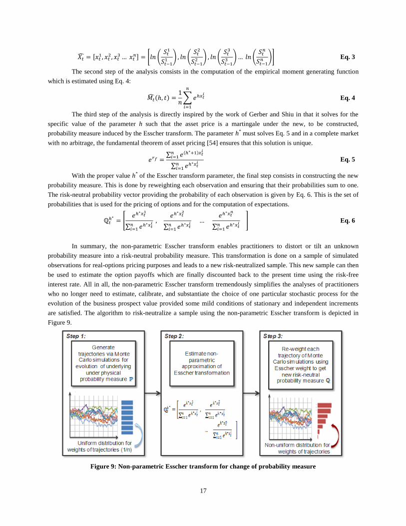
In summary, the non-parametric Esscher transform enables practitioners to distort or tilt an unknown

probability measure into a risk-neutral probability measure. This transformation is done on a sample of simulated

observations for real-options pricing purposes and leads to a new risk-neutralized sample. This new sample can then

be used to estimate the option payoffs which are finally discounted back to the present time using the risk-free

interest rate. All in all, the non-parametric Esscher transform tremendously simplifies the analyses of practitioners

who no longer need to estimate, calibrate, and substantiate the choice of one particular stochastic process for the

evolution of the business prospect value provided some mild conditions of stationary and independent increments

are satisfied. The algorithm to risk-neutralize a sample using the non-parametric Esscher transform is depicted in

Figure 9.

Figure 9: Non-parametric Esscher transform for change of probability measure

18

5.3 Resampling using the “Bootstrapping” technique

The non-parametric Esscher transform enables the change of probability measure and the derivation of a

new equivalent risk-neutral measure. By doing so, the technique changes the mean of the terminal distribution of the

business prospect value by reweighting the different outcomes. The procedure is however acting only on the

terminal distribution of the business prospect value, so what about the distributions at intermediate time-steps? As

much as the procedure is sufficient for valuing European-type options whose values depend only on the distribution

at expiration, valuing an American or a Bermudan option requires the knowledge of the business prospect value at

each and every intermediate step under the risk-neutral measure. With this issue in mind, we propose a way to

proceed forward using a resampling technique: resampling consists in drawing with replacement from a sample to

generate a new sample. For real-options use, resampling consists in using the previously risk-neutralized terminal

distribution of returns to generate new trajectories which are risk-neutral by construction. This technique is quite

popular in statistics and finance where it is called bootstrapping.

Bootstrapping is a statistical method whose name was first coined by Efron in his 1979 Rietz Lecture [55]

to describe a resampling technique used to estimate the precision of some statistics such as the mean, median, or

standard deviation of a distribution. In this case, bootstrap samples are constructed by sampling with replacement a

subset of an original distribution. The statistics of interest are then computed for each bootstrap sample and the

variability between the results can be analyzed to derive some confidence intervals for the statistics. For the problem

under investigation, the essence of the bootstrap method is retained but the application is totally different: similarly

to the original application, the bootstrap method is used to sample with replacement from an original distribution but

what is new is that the bootstrap sample is used next to generate business prospect value trajectories. In other words,

the distribution of asset prices under the historical probability measure is first risk-neutralized using the non-

parametric Esscher transform yielding a new re-weighted probability distribution. In turn, this risk-neutral

distribution under the new probability measure is sampled with replacement to yield bootstrap subsamples which are

used to construct trajectories under the risk-neutral probability measure. Another advantage of the bootstrap

technique is that the newly generated trajectories will all carry the exact same weight. The method is illustrated in

Figure 10.

Figure 10: Bootstrap method to generate trajectories

For the pricing of options, special care needs to be paid when bootstrapping: indeed, instead of simply

generating distributions, the bootstrapping is applied to simulate the realization of a stochastic process. In fact,

bootstrapping will no longer generate distributions but rather trajectories or time-indexed distributions. If the

original process to be simulated has some serial correlation properties, these would need to be accounted for in the

Step 2:

Sampling from

new population

Step 3:

Construction of trajectories using values

from sampling

Step 1:

Distribution of

observations assumed to be

new population

19

bootstrapping method since a naïve bootstrapping does not induce any serial correlation. In the following work, the

simplifying assumption of lack of serial correlation is imposed.

Provided that no serial correlation exists, another update to the method is required for the purpose of risk-

neutral trajectory generation. Indeed, bootstrapping usually starts with a sample of observations for which each

individual observation carries the exact same weight. In other words, the original sample is “uniformly distributed”

with each outcome carrying a probability of one over the sample size (1/n). However, in the current application the

outcomes of the simulation have been reweighted during the risk-neutralization process and each outcome has a

specific weight (or probability). As a result, the individual weights (or probabilities) associated with each outcome

have to be accounted for when sampling to ensure that the risk-neutral property is preserved and carried over to the

trajectories to be generated. An algorithm is proposed in Figure 11 to sample while preserving the risk-neutral

property. It consists in figuratively stacking all the weights in a column. The “height of the column” should be

exactly one since the weights represent a probability measure. A random number is then drawn to select which

“height” in the column is reached and therefore which piece of the stack is selected. By doing so, outcomes with

larger weights have a greater chance of being drawn, while outcomes with a smaller weight have less chance of

being drawn during the resampling effort.

Figure 11: Resampling from weighted observations by first stacking probabilities and then drawing

randomly from the stack (mapping between position in the stack and original outcome value is known)

5.4 American option valuation using Least-Squares Monte-Carlo technique

For real-options applications, Monte Carlo simulations enable the capture of a multitude of uncertainties

and their interdependencies. However, pricing real-options using Monte Carlo simulations has long been hindered

by the perceived inability of simulation techniques to correctly handle path-dependant options [56]. The main reason

for this difficulty is that simulations will yield an estimate of the option value at a single point defined by the current

time and the current business prospect value. The technique does not yield information regarding the option value at

future times and for different business prospect values. This is problematic. How then to ensure that the early-

exercise policy is not violated? In other words, when moving along a simulated trajectory, one needs to ensure that

the optimal early-exercise policy is followed. This means that while marching forward in time, one has to compare

the value of holding the option for at least one extra step to the payoff earned by an immediate exercise.

Mathematically, the value of the American option at the kth

time-step denoted on an asset S with observed

value and with payoff function P can be expressed as the maximum between exercising immediately and holding

Step 2:

Representation of

distribution on [0,1] scale

Step 1:

Weighted

observations(Initial population)

Step 3:

Sampling from

population with replacement

WeightsTrajectories0

1

Representation

Sample

Step 4:

Construction of

trajectories using values from sampling

Trajectory from sample

20

the option as shown in Eq. 7. The issue is that there is yet no estimate of the present value of the one-period-ahead

option value .

Eq. 7

Fortunately, this paradigm has evolved starting in 1993 with the paper of Tilley [57] which aims was to

dispel the belief that American-style options could not be valued using simulations. A significant improvement came

in 1996 with the work of Carriere [58] regarding the valuation of options with early-exercise properties. Faced with

the same problem of estimating the one-period-ahead option value for subsequent comparison with the immediate

exercise payoff, Carriere suggests the use of non-parametric regressions to regress the conditional expectation and

therefore to estimate the value of holding the options. As noted by Stentoft[59], the reason for this regression is that

a conditional expectation is a function and “any function belonging to a separable Hilbert space may be represented

as a countable linear combination of basis-functions for the space.” Consequently, let’s introduce as a family

of basis-functions for that space. The expectation may be rewritten and approximated using the first M basis-

functions as shown in Eq. 8:

Eq. 8

Any family of basis-functions should work but Carriere suggests using either splines or a polynomial

smoother. Next task is the estimation of the coefficients of the linear combination. This is done marching

backward, starting at expiration and moving back time-step by time-step until the present time: at expiration, the

value of the option is exactly the payoff while for all preceding time-steps denoted , a regression is performed

using the observations of the asset price for the N simulated trajectories at that time denoted by as well as the

option value at the following time-step . The regression objective is to select a family of coefficients

that minimizes the error between the regressed conditional expectations and the option value across all simulated

trajectories. This error is defined in Eq. 9:

Eq. 9

The immediate exercise value at time denoted is then compared to the discounted regressed

conditional expectation to find the option value, defined by Eq. 10. The procedure is repeated for each time-step and

for each trajectory until the present time to find the value of the American option.

Eq. 10

The algorithm for American option valuation using simulation and regression techniques is depicted in

Figure 12. A popular enhancement to this work is the Least-Squares Monte Carlo approach of Longstaff and

Schwartz [60]. Dating back to 2001, this approach is very similar to the method of Carriere except for two facts: the

algorithm uses a least-squares regression and the regression is made using only in-the-money paths.

In the Longstaff-Schwartz method, the proposed regression uses an ordinary least-squares technique to

regress the conditional expectation

against a set of explanatory variables. The set of explanatory

variables is a family of basis-function valued using the conditioning underlying asset price

. One may use

the simple monomial family as the family of basis-functions. Furthermore, the regression is

performed using only paths that are in-the-money since the decision to exercise or not the option is only relevant

whenever the option is in-the-money. According to Longstaff and Schwartz, “by focusing on the in-the-money

paths, [… they…] limit the region over which the conditional expectation must be estimated, and far fewer basis

functions are needed to obtain an accurate approximation to the conditional expectation function.”

21

Figure 12: American option valuation with regression

A subtle difference with the works of Carriere is the choice of realized payoffs as dependent variables for

the regression instead of using previously computed conditional expectations. These realized payoffs may be

resulting from an early exercise at the subsequent time-step or from an early exercise several steps down-the

trajectory, for instance at . According to the authors, this precludes “an upward bias in the value of the option”.

In other words, the conditional expectation at time denoted by

is used only once in the entire

algorithm: to check whether the value of holding the option is greater than the value of immediate exercise. For all

other purposes, such as the estimation of the option value at time denoted as or the regression of the

conditional expectation at time denoted by

, the conditional expectation at time is not used.

This leads to the following exercise rule and option value in Eq. 11. Let’s notice the subtle difference with Eq. 10 in

what the option value really is (the exercise rule remains the same).

Eq. 11

5.5 Summary of the proposed methodology

Having described extensively the four main steps of the proposed methodology to value real-options with

early exercise privileges, the diagram in Figure 13 summarizes the different techniques, highlights the order in

which they are used, and finally depicts the flow of information between the various steps. The proposed

methodology may seem daunting at first but each of these steps uses techniques widely used and accepted within

companies.

Step 3:

Estimate one-step

ahead conditional expectation of

option value

using least-squares

regression

T+1T

S1(t)

S2(t)

S3(t)

S4(t)

S5(t)

S1(t+1)

S2(t+1)

S3(t+1)

S4(t+1)

S5(t+1)

𝑘+1| 𝑘 = 𝑘 𝑘

=1

Step 1:

Generate

risk-neutral trajectories for

evolution of

underlying

Geometric Brownian Motion

Time

(Months)

Business Prospect Value

0

0.5

1

1.5

0 12 24 36 48 60

𝐵 𝑘𝑝𝑟𝑜𝑝 𝑔 𝑟𝑜 𝑘 𝑜 𝑘 1

Step 4:

Estimate option

value by computing maximum of

immediate exercise

and regressed discounted one-step

ahead expectation of option value

𝑘 = 𝑘 , 𝑟 𝑘+1 𝑘 𝑘+1| 𝑘

𝑘 = 𝑘 , 𝑟 𝑘+1 𝑘 𝑘+1| 𝑘

Step 2:

Estimate option

value by computing option payoff at

option expiration for

each trajectory

Geometric Brownian Motion

Time

(Months)

Business Prospect Value

0

0.5

1

1.5

0 12 24 36 48 60

𝑇

1.9

1.1

0.6

0.2

0

22

Figure 13: Main steps of proposed methodology

5.6 Meeting the Georgetown Challenge?

In the previous sections, a methodology has been constructed step by step to analyze long-term staggered

corporate investments featuring flexibility. Now would be a good time to revisit the key challenges identified earlier

in this paper and to verify whether the proposed way-forward would meet the requirements set forth by the

Georgetown Challenge (Copeland and Antikarov [25]). The Georgetown Challenge consists in a series of

requirements that real-options analyses have to meet in order to get traction and wide acceptance amongst

practitioners in the industry. These set of requirements were agreed upon during a real-options symposium held on

the campus of Georgetown University in 2003. Table 4 on the following page maps the requirements of the

Georgetown Challenges and the specific challenges identified as part of this research to the assumptions, techniques,

and solutions shaping the proposed methodology.

Uncertainty Modeling

Driving

Uncertainties

Identification

Modeling Stochastic

Processes for Uncertainties

StepI.a

Investment

Boundaries

Comparison of

current State of

Business

Definition of Optimal Conditions

for Investment in Program

Step IV.b

Generating

Trajectories for

Program Economic

Value

Revenue Estimation

Simulation of Stochastic

Process for Program Value Evolution

StepI.b

Re-sampling Method

(Bootstrapping)

New Risk-Neutral

Trajectories for Program Economic

Value

Simulation of Risk-Neutral

Process for Program Value Evolution

Step III Non parametric

Esscher Transform

Risk-Neutral

Distribution of

Program Economic

Value Returns

Risk-Neutral Distribution of

Program Value Returns

Step II

Least Squares

Monte Carlo

Regression

Investment Policy

Investigation of Investment

Timeline for Staggered Program

Step

IV.a

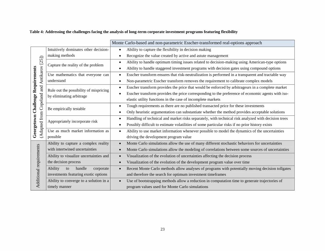
23

Table 4: Addressing the challenges facing the analysis of long-term corporate investment programs featuring flexibility

Monte Carlo-based and non-parametric Esscher-transformed real-options approach

Geo

rget

ow

n C

hall

enge

Req

uir

emen

ts

(Adap

ted f

rom

Copel

and a

nd A

nti

kar

ov [

25])

Intuitively dominates other decision-

making methods

Ability to capture the flexibility in decision making

Recognize the value created by active and astute management

Capture the reality of the problem Ability to handle optimum timing issues related to decision-making using American-type options

Ability to handle staggered investment programs with decision gates using compound options

Use mathematics that everyone can

understand

Esscher transform ensures that risk-neutralization is performed in a transparent and tractable way

Non-parametric Esscher transform removes the requirement to calibrate complex models

Rule out the possibility of mispricing

by eliminating arbitrage

Esscher transform provides the price that would be enforced by arbitrageurs in a complete market

Esscher transform provides the price corresponding to the preference of economic agents with iso-

elastic utility functions in the case of incomplete markets

Be empirically testable Tough requirements as there are no published transacted price for these investments

Only heuristic argumentation can substantiate whether the method provides acceptable solutions

Appropriately incorporate risk Handling of technical and market risks separately, with technical risk analyzed with decision trees

Possibly difficult to estimate volatilities of some particular risks if no prior history exists

Use as much market information as

possible

Ability to use market information whenever possible to model the dynamics of the uncertainties

driving the development program value

Ad

dit

ion

al r

equir

emen

ts Ability to capture a complex reality

with intertwined uncertainties

Monte Carlo simulations allow the use of many different stochastic behaviors for uncertainties

Monte Carlo simulations allow the modeling of correlations between some sources of uncertainties

Ability to visualize uncertainties and

the decision process

Visualization of the evolution of uncertainties affecting the decision process

Visualization of the evolution of the development program value over time

Ability to handle corporate

investments featuring exotic options

Recent Monte Carlo methods allow analyses of programs with potentially moving decision tollgates

and therefore the search for optimum investment timeframes

Ability to converge to a solution in a

timely manner

Use of bootstrapping methods allow a reduction in computation time to generate trajectories of

program values used for Monte Carlo simulations

24

6 Verification and Validation

In this section, the proposed methodology is validated for different test cases against known results from

plain vanilla options. Since the “pricing” part of the proposed methodology is validated, there is no need to set-up a

real-options scenario and instead the validation is performed by comparing the results of the proposed methodology

to known results for financial options. The test cases involve different sets of put and call options of both European

and American types.

6.1 European options

In order to test the methodology using European options, the last step using the Least-Squares Monte Carlo

is changed. Indeed, since there is no need to compare the one-step ahead conditional expectation to the value of

exercising early, the regression-based Least-Squares Monte Carlo technique is removed and replaced with a simpler

payoff estimation at maturity of the option. The results are displayed in Table 5 for an underlying following a

geometric random walk with a drift of 8.5% under the physical probability measure. The results from the proposed

methodology are based on a simulation of 50,000 paths and are in agreement with the closed-form solution.

Table 5: Comparison of proposed valuation and closed-form formula for European call (a) and put (b)

options

6.2 American options

To test the methodology using American options, the entire methodology is now used. The results are

displayed in Table 6. They exhibit on average good results when compared to results obtained from the partial-

differential equation approach. There are however some discrepancies, in particular for out-of-the-money options,

between the two valuation methods. These discrepancies are probably due to errors introduced by the least-squares

regression. Further investigations on the selection of basis-functions and on the number of functions to use might

help achieve better results.

25

Table 6: Comparison of proposed valuation and PDE solution for American call (a) and put (b) options

7 Performance Improvement Package Evaluation

The proposed methodology is applied to the evaluation of the performance improvement package presented

previously in this paper. However, the development of the performance improvement package is simplified for this

validation so as not to over-complicate the problem with unnecessary burden. Instead of studying the four successive

nested real-options, the paper will focus on a single option which is the option to fund the detailed development

phase once more information has been obtained after the initial market research. This helps avoids having to

perform time-consuming simulations on simulations to evaluate nested options.

7.1 Value of the development of the Performance Improvement Package (PIP)

The computation of the development program value is articulated around two steps. In the first step, an

estimate of the sales given the current state of the uncertainties is estimated. This is done using a market model

described in Justin, Briceno, and Mavris [42]. This market model estimates the market penetration by first

computing the net present value of the aircraft featuring the performance improvement package, and by comparing

this value to the value of the same aircraft without the PIP and to the value of other competing aircraft. This

evaluation is performed for different missions representing different types of airlines and therefore different market

segments. Decision choice analysis is then applied to estimate market preferences on these different segments. In the

second step of the analysis, the market preference is used to estimate the revenues and profits stemming from the

sales of the Performance Improvement Package to the airlines. This enables the evaluation of the development

program value.

Table 7: Market Assumption for Performance Improvement Package

Overall market size 100 Units/Year

Length of PIP program 8 Years

Market value leakages -15% per year

Revenues per unit (Normalized) 0.045 2014-US$

Cost per unit (Normalized) 0.040 2014-US$

WACC (Typical Airframer) 13.5% per year

Maturity Strike/Spot PDE ApproachSimulation &

NP EsscherError Maturity Strike/Spot PDE Approach

Simulation &

NP EsscherError

0.5 0.8 0.20490 0.20583 -0.45% 0.5 0.8 0.00000 0.00001 /0.5 0.9 0.10870 0.1084 0.28% 0.5 0.9 0.00140 0.00112 -20.00%0.5 1 0.03260 0.03449 -5.80% 0.5 1 0.02390 0.02405 0.63%0.5 1.1 0.02800 0.00398 85.77% 0.5 1.1 0.10000 0.10007 0.07%0.5 1.2 0.00010 0.00022 -120.00% 0.5 1.2 0.20000 0.19980 -0.10%1 0.8 0.20960 0.21590 -3.01% 1 0.8 0.00020 0.00018 -11.35%1 0.9 0.11890 0.11944 -0.45% 1 0.9 0.00480 0.00460 -4.10%1 1 0.04840 0.04876 -0.74% 1 1 0.03150 0.03172 0.70%1 1.1 0.01330 0.01325 0.38% 1 1.1 0.10090 0.10062 -0.28%1 1.2 0.00210 0.00225 -7.14% 1 1.2 0.20000 0.19973 -0.14%2 0.8 0.21930 0.22114 -0.84% 2 0.8 0.00150 0.00147 -2.00%2 0.9 0.13700 0.14198 -3.64% 2 0.9 0.01050 0.01034 -1.52%2 1 0.07210 0.08057 -11.74% 2 1 0.04040 0.03784 -6.34%2 1.1 0.03180 0.03155 0.79% 2 1.1 0.10360 0.10308 -0.50%2 1.2 0.01180 0.01295 -9.75% 2 1.2 0.20000 0.19923 -0.39%

(a) American Call Option ( Drift=8.5%,Div= 4.0%, Rf=5.0%, Vol=10%) (b) American Put Option ( Drift=8.50%, Div=4.0%, Rf=5.00%, Vol=10%)

26

7.2 Uncertainty quantification and modeling

The development of complex aerospace systems-of-systems and the extensive certification processes lead

to long development timelines which exacerbate the effects of uncertainty. Uncertainty might be split into two

categories. One category is for technical uncertainty over which manufacturers have some control (such as

performance estimates and development schedules). Manufacturers may be able to limit the adverse effects of

technical uncertainty by implementing mostly mature technologies in their designs or by using conservative

estimates, and possibly by using probabilistic techniques during design. The other category is for market uncertainty

which manufacturer do not control (such as market size and commodity prices). Owing to this lack of control,

aircraft manufacturers must come up with solutions to hedge against these types of uncertainties to ensure that their

decision-making process is optimal and robust regardless of the evolution of the underlying uncertain parameters.

Numerous market uncertainties affect manufacturers but only a few have profound effects on the viability

of large aerospace development programs. One of them is the price of jet-fuel which drives the need for new more

efficient aircraft to replace older ones since fuel-related expenditures account for about forty percent of aircraft

direct operating costs. Consequently, increasing fuel prices have dramatic effects on the profitability of airlines and

put pressure on airlines to renew their fleets. Another uncertainty which may have some impact in the future is the

taxation of carbon dioxide emissions. Little information regarding the effects of such regulations on aircraft

manufacturers is available due to the newness of the taxation scheme. Indeed, the European Union has recently set-

up the Emissions Trading Scheme (ETS) whereby airlines may have to buy permits for roughly fifteen percent of

their carbon dioxide emissions.

7.2.1 Uncertain jet-fuel costs

The jet-fuel price analysis is performed using data from the United States Energy Information

Administration representing the historical time series of U.S. Gulf Coast kerosene-type jet-fuel spot price. The time

series is plotted in Figure 14 and looks similar to many financial time series with high volatility and no obvious

autocorrelation structure.

Figure 14: (a) Closing price of jet-fuel; (b) Continuously compounded daily jet-fuel price returns

Inspection of the time series in Figure 14 indicates a bell-shaped distribution of the returns centered on zero

with some clustering of high volatility as shown in Figure 15. Despite this heteroscedasticity, a stochastic model

similar to a random walk, the Geometric Brownian Motion (GBM) is hypothesized.

27

Figure 15: Distribution of daily jet-fuel price returns

Several statistical tests are run to check whether this assumption can be rejected at the usual 5% level of

significance. The first test is the variance ratio test as described by Campbell et al.[61]. This test checks the

correlation structure of the increments. Under the GBM assumptions, the increments are uncorrelated. The

autocorrelation is studied at lags 2, 4, 8 and 16 days, and for each analysis, the test fails to reject the GBM

assumption. The second test is the Cowles-Jones Ratio test described again in [61] which checks whether the

increments are independent and identically distributed. Under the GBM assumption, the increments are independent

and identically distributed. This test also fails to reject the GBM assumption which means that the apparent

heteroscedasticity previously observed is not significant enough. Based on these results, a geometric Brownian

motion is used to model the stochastic process driving the price of jet-fuel. The stochastic differential equation is

given in Eq. 12 with the Wiener process (Wt), the spot price (St), the yearly drift ( ) and the yearly volatility ( ).

Eq. 12

7.2.2 Uncertain emission costs

The Emissions Trading Scheme may require airlines to buy permits for about fifteen percent of the airlines’

carbon dioxide emissions. These permits are in limited quantity and may be purchased on the carbon market in the

form of European Union Allowances (EUA). For instance, Air France started using the BlueNext exchange platform

in 2012 to buy EUAs on the spot market [62]. The carbon emission analysis is therefore performed using the BNS

EUA 08-12 time series available on the Bluenext exchange website for data from February 2008 to June 2012. Like

the previous example, the time series plotted in Figure 16 exhibits high volatility, with no obvious autocorrelation

structure but with a downward trend.

Figure 16: (a) Closing price of EUA; (b) Continuously compounded daily EUA price returns

Inspection of the time series displayed in Figure 16 indicates a bell-shaped distribution of the returns

centered on zero with some clustering of high volatility, as shown in Figure 17. Based on these observations, a

geometric Brownian motion is hypothesized.

28

Figure 17: Distribution of daily EUA price returns

The same statistical tests are run to check whether the GBM assumption can be rejected at the 5% level of

significance. The variance ratio test is run for lags 2, 4, 8 and 16 days, and each time, the GBM assumption cannot

be rejected. The Cowles-Jones Ratio test is run and also fails to reject the GBM assumption. Based on these results,

a geometric Brownian motion is used to model the stochastic process driving the price of carbon allowances and its

parameters are provided in Eq. 13.

Eq. 13

7.2.3 Treatment of correlations

The two stochastic processes retained for the modeling of jet-fuel price and carbon emission cost

uncertainties are independent models. However, a more intricate relationship between the two models is likely.

Indeed, a period of strong growth in Europe may result in higher demand for air transportation and therefore higher

prices for jet-fuel. Similarly, this higher demand for air transportation may result in more demand for carbon permits

and therefore higher emission allowance prices. The relationship between the price of jet-fuel and the price of

carbon permits can be captured with the correlation matrix. This matrix is estimated by first cleaning the time series

to ensure that quotes are available for both on the same date and then estimating the correlation between the

continuous returns of each time series. The correlation matrix is given in Eq. 14 and indicates a correlation of 19%

between the two data series.

Eq. 14

To include this correlation in the two stochastic models previously defined, correlated numbers need to be

sampled from the standard normal distribution used in the geometric Brownian motion. This is performed using a

Cholesky decomposition of the correlation matrix as shown in Eq. 15. The positive definite correlation matrix is

decomposed to give a lower-triangular matrix which, when applied to a vector of uncorrelated samples, produces a

sample vector with the correlation properties of the system being modeled.

Eq. 15

7.3 Results

The results from the real options analysis are summarized in Table 8 and Figure 18. Since simulation is used

to estimate the option price and since there is always some randomness left in the results, the computation has been

repeated 160 times which helps gauge the spread of results. Using a real-options analysis, the program does have

29

value and would be undertaken. This is in stark contrast with the results from a deterministic discounted cash flow

analysis which would lead to an abandonment of the project.

Table 8: Value of Performance Improvement

Package with and without flexibility

Figure 18: Distribution of PIP program values

8 Conclusion

In this research, a new methodology for the analysis of the economic performance of development

programs in the aerospace industry is proposed. By cross-fertilizing elements from financial engineering, actuarial

sciences, and statistics, this research has enabled the development of a traceable and transparent framework for the

analysis of staggered corporate investments featuring timing flexibility. Most of the techniques shaping this

methodology are well accepted and already in use in the aerospace community which may help acceptance by

practitioners. The methodology is articulated around four main points: a simulation of the evolution of the value of a

business prospect over time under the physical probability measure, a non-parametric risk-neutralization to yield a

distribution of the business prospect value under the equivalent martingale measure, a resampling to yield risk-

neutral business prospect value evolution over time with equal weight for each trajectory, and finally an option

valuation exercise using regression to value a real-option featuring timing flexibility and to estimate the early-

exercise boundary. Next, the methodology is tested against different cases of known vanilla options. Finally, the

methodology is applied to evaluate the development, certification, and testing of a technology package to improve

the economics of commercial aircraft in operations.

Several improvements could be achieved using slight modifications of the proposed methodology. The first

one is to use quasi-Monte Carlo simulation to improve the generation of random numbers. The well-known Halton

as well as the Sobol sequences could be used to generate random numbers which may be more uniformly distributed

than the random number generator implemented in the spreadsheet software used. Another improvement would

include the review of other families of basis functions for use in the Least-Squares Monte Carlo regressions.

Including more than three terms may also improve the regression fit when computing the conditional expectation.

Furthermore, resampling using the bootstrapping technique precludes the capture of serial correlations, and

more generally autocorrelations, when simulating the evolution of the business prospect value. Future work will

include further literature review to improve the current bootstrapping technique to be able to capture serial

correlations. This may significantly extend the domain of application of the proposed methodology.

References

[1] P. Clark, Buying the Big Jets, 2nd ed., Ashgate, 2007.

[2] C. Justin, "Investigation on the use of real-options analysis and competitive analysis to detect trigger events for

successful aerospace research and development programs," 2013.

[3] G. Norris, More MD-11 improvements revealed, 1995.

DCF analysis of PIP program -0.7002

PIP Program value with options 0.2901

Standard deviation of PIP values 0.0124

PIP Program Value

(Normalized by Initial Investment)

0

10

20

30

40

50

60

Fre

qu

en

cy

PIP Program Value

30

[4] CFM, CFM56-5B PIP for the Airbus A320 family, Retrieved November 23rd 2013.

[5] K. Thomson and E. T. Schulze, Delivering fuel and emissions savings for the 777, 2009.

[6] Airbus, Airbus launches Sharklet retrofit for in-service A320 family aircraft, 2013.

[7] J. Graham and C. Harvey, "The theory and practice of corporate finance: evidence from the field," Journal of

Financial Economics, vol. 60, pp. 187-243, 2001.

[8] A. Dixit and R. Pindyck, Investment under uncertainty, Princeton University Press, 1994.

[9] S. C. Myers, "Determinants of corporate borrowing," Journal of Financial Economics , vol. 5, no. 2, pp. 147-

175, 1977.

[10] F. Black and M. Scholes, "The pricing of options and corporate liabilities," Journal of Political Economy, vol.

81, no. 3, pp. 637-654, May - Jun 1973.

[11] R. C. Merton, "Theory of rational option pricing," The Bell Journal of Economics and Management Science,

vol. 4, no. 1, pp. pp. 141-183, 1973.

[12] C. Krychowski, "Apport et limites des options réelles à la décision d’investissement stratégique : une étude

appliquée dans le secteur des télécommunications," 2007.

[13] H. Smit and L. Trigeorgis, Strategic Investment: Real Options and Games, Prin, 2004.

[14] J. Stonier, "What is an aircraft purchase option worth? Quantifying asset flexibility created through

manufacturer lead-time reductions and product commonality," Handbook of Airline Finance, 1999.

[15] I. Fernandez-Martin, "Valuation of design adaptability in aerospace systems," 2008.

[16] B. Miller and J.-P. Clarke, "Investments under uncertainty in air transportation," Journal of the Transportation

Research Forum, vol. 44, pp. 61-74, Spring 2005.

[17] V. Datar and S. Mathews, "European real options: an intuitive algorithm for the Black-Scholes formula,"

Journal of Applied Finance, vol. 14, p. 45, Spring 2004.

[18] S. Mathews, "Valuing risky projects with real options," Research-Technology Management, vol. 52, 2009.

[19] B. Miller and J.-P. Clarke, "Strategic guidance in the development of new aircraft programs: a practical real

options approach," IEEE Transaction on Engineering Management, vol. 55, pp. 566-578, November 2008.

[20] T. Luehrman, "Investment opportunities as real options: getting started on the numbers," Harvard Business

Review, vol. Case 9, July-August 1998.

[21] J. Shank and D. Peterson, "Strategic cost analysis for capital spending decisions," Cost Management, vol. 19, p.

14, 2005.

[22] T. Copeland, T. Koller and J. Murrin, Valuation. Measuring and managing the value of companies, Third

Edition ed., McKinsey, 2000.

[23] T. Copeland and V. Antikarov, Real options - a practitioner's guide, Texere, 2001.

[24] A. Borison, "A response to "Real options: meeting the Georgetown challenge"," Journal of Applied Corporate

Finance, vol. 17, pp. 52-54, Spring 2005.

[25] T. Copeland and V. Antikarov, "Real options: Meeting the Georgetown challenge," Journal of Applied

Corporate Finance, vol. 17, pp. 32-51, 2005.

[26] P. Samuelson, "Proof that properly anticipated prices fluctuate randomly," Industrial Management Review, vol.

6, pp. 41-49, 1965.

[27] A. Kemna, "Case studies on real options," Financial Management, vol. 22, pp. 259-270, 1993.

[28] H. Weeds, "Strategic delays in a real options model of R\&D competition," The Review of Economic Studies,

vol. 69, pp. 729-747, 2002.

[29] A. Borison, "Real options analysis: where are the Emperor's clothes?," Journal of Applied Corporate Finance,

vol. 17, pp. 17-31, 2005.

[30] R. McDonald and D. Siegel, "The value of waiting to invest," The Quarterly Journal of Economics, pp. 707-

727, 1986.

[31] S. Grenadier, "Valuing lease contracts: a real-options approach," Journal of Financial Economics, vol. 38, pp.

297-331, 1995.

[32] S. Majd and R. Pindyck, "Time to build, option value and investment decisions," Journal of Financial

31

Economics, vol. 18, pp. 7-27, 1987.

[33] M. Dias and k. Rocha, "Petroleum concessions with extensible options using mean resersion with jumps to

model oil prices," 1999.

[34] L. Trigeorgis, "Evaluating leases with complex operating options," European Journal of Operational Research,

vol. 91, pp. 315-329, 1996.

[35] N. Lewis, D. Enke and D. Spurlock, "Valuation for the strategic management of research and development

projects: the deferral option," Engineering Management Journal, vol. 16, pp. 36-48, 2004.

[36] S. Rose, "Valuation of interacting real options in a tollroad infrastructure project," The Quarterly Review of

Economics and Finance, vol. 38, pp. 711-723, 1998.

[37] C.-L. Tseng and G. Barz, "Short-term generation asset valuation: a real options approach," Operations

Research, vol. 50, pp. 297-310, 2002.

[38] N. Metropolis and S. Ulam, "The Monte Carlo method," Journal of the American Statistical Association, vol.

44, pp. 335-341, 1949.

[39] P. Boyle, "Options: a Monte Carlo approach," Journal of Financial Economics, vol. 4, pp. 323-338, 1977.

[40] M. Broadie and P. Glasserman, "Estimating security price derivatives using simulation," Management Sciences,

vol. 42, pp. 269-285, 1996.

[41] P. Glasserman, Monte Carlo methods in financial engineering, Rozovskii and Yor, Eds., Springler-Verlag,

2004.

[42] C. Justin, S. Briceno and D. Mavris, "A competitive and real-options framework for the economic analysis of

large aerospace programs," ICAS, Brisbane, QLD, 2012.

[43] E. Fama, "The behavior of stock-market prices," Journal of Business, vol. 38, pp. 34-105, 1965.

[44] H. Gerber and E. Shiu, "Option pricing by Esscher transforms," Transactions of Society of Actuaries, vol. 46,

pp. 99-141, 1994.

[45] F. Esscher, "On the probability function in the collective theory of risk," Scandinavian Actuarial Journal, vol.

3, pp. 175-195, 1932.

[46] P. M. Kahn, "An introduction to collective risk theory and its application to stop-loss reinsurance,"

Transactions of Society of Actuaries, vol. 14, pp. 400-449, 1962.

[47] Y. Miyahara, "A note on Esscher transformed martingale measures for geometric Levy processes," 2004.

[48] H. Follmer and M. Scheizer, Encyclopedia of quantitative finance, Wiley, 2010, pp. 1200-1204.

[49] M. Frittelli, "Minimal entropy criterion for pricing in one period incomplete markets," 1995.

[50] H. Gerber and E. Shiu, "Martingale approach to pricing perpetual american options," Astin Bulletin, vol. 24, pp.

195-220, November 1994.

[51] D. Cass and J. Stiglitz, "the structure of investor preferences and asset returns, and seprability in portfolio

allocation: a contribution to the pure theory of mutual funds," Journal of Economic Theory, vol. 2, pp. 122-160,

1970.

[52] J. Stiglitz, "Theory of valuation: frontiers of modern financial theory," S. Bhattacharya and G. Constantinides,

Eds., Rowman \& Littlefield Publishers, 1988, pp. 342-356.

[53] M. Pereira, C. Epprecht and A. Veiga, "Option pricing via nonparametric Esscher transform," Marseille,

France, 2011.

[54] J. M. Harrison and D. M. Kreps, "Martingales and arbitrage in multiperiod securities markets," Journal of

Economic Theory, vol. 20, pp. 281-408, 1979.

[55] B. Efron, "Bootstrap methods: another look at the jackknife," The Annals of Statistics, vol. 7, pp. 1-26, 1979.

[56] J. Hull, Options, futures and other derivatives securities, 2nd in 1993, 6th ed., Prentice Hall, 2006.

[57] J. A. Tilley, "Valuing American options in a path simulation model," Transactions of the Society of Actuaries,

vol. 45, pp. 83-104, 1993.

[58] J. Carriere, "Valuation of the early-exercise price for options using simulations and non-parametric regression,"

Insurance: Mathematics and Economics, vol. 19, pp. 19-30, 1996.

[59] L. Stentoft, Value function approximation or stopping time approximation: a comparison of two recent

numerical methods for American option pricing using simulation and regression, 2008.

32

[60] F. Longstaff and E. Schwartz, "Valuing American options by simulation: a simple least-square appr," The

Review of Financial Studies, vol. 14, pp. 113-147, 2001.

[61] J. Y. Campbell, A. W. Lo and A. C. MacKinlay, The econometrics of financial markets, Princeton University

Press, 1997.

[62] M. Szabo, Airlines alliances take cartel approach to carbon trading, 2012.

Valuation of Real Options with Flexible Early Exercise in ... · Valuation of Real Options with...

Documents

Transcript of Valuation of Real Options with Flexible Early Exercise in ... · Valuation of Real Options with...