Valuation and Financing of

Early Stage Technological Companies:

Analysis with a Real Options Structural Model

Daniel Freire da Fonseca

Thesis to obtain the Master of Science Degree in

Industrial Engineering and Management

Supervisor: Prof. João Manuel Marcelino Dias Zambujal de Oliveira

Examination Committee

Chairperson: Prof. Francisco Miguel Garcia Gonçalves de Lima

Members of the Committee: Prof. Maria Margarida Martelo Catalão Lopes de Oliveira

Pires Pina

Prof. Maria Isabel Craveiro Pedro

December 2015

i

ii

Acknowledgments

Solitary though a work like this may be, it would not be, at all, without your help.

A sincere thank you to Professor João Zambujal de Oliveira, who guided me from the absence of a

project, through too many ideas and finally to a viable work.

To you, Raquel, I owe nothing short of unending gratitude for your tireless support and contribution.

A special thank you to Vasco Rato for his help in improving my programming skills.

Finally to my parents, who sustain and support me, making possible my academic journey; thankfully

completed.

iii

iv

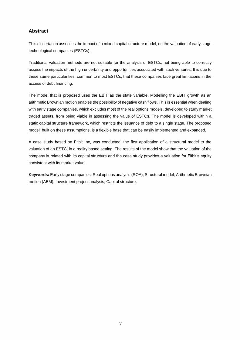
Abstract

This dissertation assesses the impact of a mixed capital structure model, on the valuation of early stage

technological companies (ESTCs).

Traditional valuation methods are not suitable for the analysis of ESTCs, not being able to correctly

assess the impacts of the high uncertainty and opportunities associated with such ventures. It is due to

these same particularities, common to most ESTCs, that these companies face great limitations in the

access of debt financing.

The model that is proposed uses the EBIT as the state variable. Modelling the EBIT growth as an

arithmetic Brownian motion enables the possibility of negative cash flows. This is essential when dealing

with early stage companies, which excludes most of the real options models, developed to study market

traded assets, from being viable in assessing the value of ESTCs. The model is developed within a

static capital structure framework, which restricts the issuance of debt to a single stage. The proposed

model, built on these assumptions, is a flexible base that can be easily implemented and expanded.

A case study based on Fitbit Inc, was conducted, the first application of a structural model to the

valuation of an ESTC, in a reality based setting. The results of the model show that the valuation of the

company is related with its capital structure and the case study provides a valuation for Fitbit’s equity

consistent with its market value.

Keywords: Early stage companies; Real options analysis (ROA); Structural model; Arithmetic Brownian

motion (ABM); Investment project analysis; Capital structure.

v

vi

Resumo

A presente dissertação estuda o impacto de uma estrutura de capital mista, na avaliação de

empresas tecnológicas em fase inicial de atividade (ETFIAs).

Os métodos tradicionais de avaliação não são os mais adequados à análise das ETFIAs, dado que

não permitem estimar corretamente o impacto da elevada incerteza e grandes oportunidades de

crescimento associadas a estas empresas. Estas mesmas especificidades, comuns à maioria das

ETFIAs, que causam consideráveis restrições no acesso a dívida por parte destas empresas.

O modelo proposto usa o EBIT como variável de estado. Modelar o crescimento do EBIT como um

movimento Browniano aritmético permite a existência de valores negativos. Este fator é essencial

quando se analisam empresas em fase inicial de atividade e exclui grande parte dos modelos de

opções reais, desenvolvidos para estudar ativos negociados nos mercados, de entre as opções

viáveis para avaliar ETFIAs. O modelo é desenvolvido assumindo uma estrutura de capital estática, o

que restringe a emissão de dívida a uma única fase. O modelo assim definido é uma base flexível,

fácil de implementar e expandir.

Foi desenvolvido um caso de estudo baseado na Fitbit Inc. a primeira aplicação de um modelo

estrutural à avaliação financeira de uma ETFIA, baseado em dados reais. Os resultados do modelo

mostram que a avaliação da empresa está relacionada com a sua estrutura de capital, e a avaliação

feita pelo modelo para o capital próprio da Fitbit é consistente com o seu valor de mercado

Palavras-chave: Empresas em fase inicial de atividade; Análise de opções reais (AOR); Modelos

estruturais; Movimento Browniano aritmético; Análise de projetos de investimento; Estrutura de capital.

vii

Table of Contents

Acknowledgments .......................................................................................................................... ii

Abstract .......................................................................................................................................... iii

Table of Contents ......................................................................................................................... vii

Figures List .................................................................................................................................... xi

Equations List .............................................................................................................................. xiii

Acronyms List ............................................................................................................................... xv

1. Introduction ................................................................................................................................ 1

1.1. Context and Relevance .............................................................................................................. 1

1.2. Objectives and Motivation........................................................................................................... 2

2. Problem Definition ..................................................................................................................... 3

3. Literature Review ....................................................................................................................... 4

3.1. Investment Cycle and Early Stage Technological Companies ................................................... 4

3.2. Intangible Assets and Intellectual Property ................................................................................ 6

3.3. Sources of Finance ..................................................................................................................... 7

Equity Financing ............................................................................................................... 7

IP Focused Debt Financing .............................................................................................. 8

IP Sale and Lease Back ................................................................................................... 8

3.4. IP Valuation ................................................................................................................................ 9

Cost Approach .................................................................................................................. 9

Market Approach .............................................................................................................. 9

Income Approach ........................................................................................................... 10

viii

a. Discounted Cash Flow model ....................................................................... 10

b. Relief from Royalty method .......................................................................... 10

Real Options Approach .................................................................................................. 10

3.5. Investment Project Valuation .................................................................................................... 11

Discounted Cash Flow ................................................................................................... 11

Net Present Value ............................................................................................. 11

Weighted Average Cost of Capital .................................................................... 11

Cost of Equity .................................................................................................... 12

Cost of Debt ....................................................................................................... 13

3.6. Real Option Analysis ................................................................................................................ 13

Call Options .................................................................................................................... 14

Put Options ..................................................................................................................... 15

Variables of Option Value ............................................................................................... 15

American and European Options ................................................................................... 16

Option Pricing Models .................................................................................................... 16

Binomial Model .................................................................................................. 16

Stochastic Differential Equations ....................................................................... 17

Black-Scholes Model ......................................................................................... 18

Considerations for Real Options .................................................................................... 19

Investment Opportunities as Real Options ..................................................................... 20

a. Option to abandon ........................................................................................ 20

b. Option to delay ............................................................................................. 20

c. Option to expand .......................................................................................... 20

d. Other options ................................................................................................ 21

Structural Models............................................................................................................ 21

4. Methodology ............................................................................................................................ 23

4.1. Main assumptions of the valuation model ................................................................................ 23

ix

Earnings Before Interest & Tax (EBIT): The project variable ......................................... 23

Arithmetic Brownian Motion: Modelling Earnings Before Interest & Tax ........................ 24

4.2. Development of a Structural Model .......................................................................................... 25

Value of a claim to cash flows following ABM ................................................................ 25

Value of unlevered ESTCs ............................................................................................. 27

Optimal capital structure for ESTCs ............................................................................... 29

Option to Invest in an ESTC ........................................................................................... 32

5. Case Study – Fitbit Inc. ........................................................................................................... 35

5.1. Overview of the company ......................................................................................................... 35

5.2. Financial data ........................................................................................................................... 36

5.3. EBIT Simulation ........................................................................................................................ 37

5.4. Model Parameters .................................................................................................................... 40

Risk free rate (𝒓) ............................................................................................................. 40

EBIT (𝒙) .......................................................................................................................... 41

Drift and standard deviation (𝝁𝒎, 𝝈) ............................................................................... 41

Tax rate (𝝉) ..................................................................................................................... 41

Risk Premium (𝜱) ........................................................................................................... 41

Investment Cost and Equity Stake (𝑰𝑪, 𝝀) ...................................................................... 42

Closure and Bankruptcy Costs (𝑪, 𝜶) ............................................................................. 42

Opportunity cost (𝜹) ........................................................................................................ 42

5.5. Model Results ........................................................................................................................... 43

Unlevered Company ....................................................................................................... 43

Optimally Levered Company .......................................................................................... 43

5.6. Sensitivity Analysis and Model Robustness ............................................................................. 44

EBIT Level ...................................................................................................................... 44

x

Drift ................................................................................................................................. 45

Volatility .......................................................................................................................... 46

Risk free rate .................................................................................................................. 47

Tax Rate ......................................................................................................................... 48

Debt ................................................................................................................................ 48

Bankruptcy Stake ........................................................................................................... 49

Investment Costs ............................................................................................................ 50

6. Conclusions ............................................................................................................................. 52

7. Bibliography ............................................................................................................................. 54

8. Annexes .................................................................................................................................... 58

8.1. Annex 1 ..................................................................................................................................... 58

8.2. Annex 2 ..................................................................................................................................... 58

xi

Figures List

Figure 1 – Components of S&P 500 Market Value (Adapted from: Malakawski, 2004) ......................... 1

Figure 2 – Investment Cycle (Adapted from Wikipedia Commons, 2009) .............................................. 4

Figure 3 – Performance of companies with the highest patent scores Versus S&P 500

(Adapted from: Malakawski, 2004) .......................................................................................................... 6

Figure 4 – Payoff Diagram for a Call Option (Adapted from: Damodaran, 2012) ................................. 14

Figure 5 – Payoff Diagram for a Put Option (Adapted from: Damodaran, 2012) .................................. 15

Figure 6 – Binomial Lattice (Adapted from: Brandão, 2005) ................................................................. 17

Figure 7 – Drift convergence…………………………………………………………………………………..37

Figure 8 – Standard deviation convergence.......................................................................................... 37

Figure 9 – Fitbit’s EBIT simulation using Arithmetic Brownian Motion (in Million US dollars) ............... 38

Figure 10 – Cumulative probability plot of the simulated EBIT (in million US dollars) .......................... 39

Figure 11 – Probability density plot of the simulated EBIT (in million US dollars) ................................ 39

Figure 12 – US 30 year Treasury Bond yields (%) (US Department of the Treasury, 2015) ................ 40

xii

Tables List

Table 1 – Fitbit’s annual financial data (Fitbit, 2015) ............................................................................. 36

Table 2 – Fitbit’s quarterly financial data (1) (Fitbit, 2015) .................................................................... 36

Table 3 – Fitbit’s quarterly financial data (2) (Fitbit, 2015) .................................................................... 37

Table 4 – Convergence analysis ........................................................................................................... 37

Table 5 – Consistency analysis ............................................................................................................. 38

Table 6 – Complete input parameters ................................................................................................... 43

Table 7 – Model Results – Unlevered Company ................................................................................... 43

Table 8 – Model Results – Optimally Leveraged Company .................................................................. 44

Table 9 – Sensitivity Analysis to 𝑥 (absolute values) ............................................................................ 44

Table 10 – Sensitivity Analysis to 𝑥 (percentage values) ...................................................................... 45

Table 11 – Sensitivity Analysis to 𝜇𝑚 (absolute values) ....................................................................... 45

Table 12 – Sensitivity Analysis to 𝜇𝑚 (percentage values) ................................................................... 45

Table 13 – Sensitivity Analysis to 𝜎 (absolute values) .......................................................................... 46

Table 14 – Sensitivity Analysis to 𝜎 (percentage values) ...................................................................... 46

Table 15 – Sensitivity Analysis to 𝑟 (absolute values) .......................................................................... 47

Table 16 – Sensitivity Analysis to 𝑟 (percentage values) ...................................................................... 47

Table 17 – Sensitivity Analysis to 𝜏 (absolute values)........................................................................... 48

Table 18 – Sensitivity Analysis to 𝜏 (percentage values) ...................................................................... 48

Table 19 – Evolution of the debt to equity ratio with growing EBIT ....................................................... 49

Table 20 – Sensitivity Analysis to 𝛼 (absolute values) .......................................................................... 49

Table 21 – Sensitivity Analysis to 𝛼 (percentage values) ...................................................................... 49

Table 22 - Sensitivity Analysis to 𝐼𝐶 (absolute values) ......................................................................... 50

Table 23 – Sensitivity Analysis to 𝐼𝐶 (percentage values) .................................................................... 50

Table 24 – Comparative relevance of the input parameters in the results of the model ...................... 51

xiii

Equations List

Equation 1 – Net Present Value ............................................................................................................ 11

Equation 2 – Value of an asset using DCF ........................................................................................... 11

Equation 3 – Weighted Average Cost of Capital ................................................................................... 12

Equation 4 – Cost of Equity ................................................................................................................... 12

Equation 5 – Beta .................................................................................................................................. 12

Equation 6 – Procedure for Accounting Beta ........................................................................................ 13

Equation 7 – Interest Coverage Ratio ................................................................................................... 13

Equation 8 – Option Delta ..................................................................................................................... 17

Equation 9 – Value of a Call using the BOPM....................................................................................... 17

Equation 10 – Arithmetic Brownian Motion ........................................................................................... 18

Equation 11 – Geometric Brownian Motion ........................................................................................... 18

Equation 12 - Black Scholes Option Pricing Model ............................................................................... 19

Equation 13 – Put - Call Parity Theorem ............................................................................................... 19

Equation 14 – Arithmetic Brownian Motion (repeated) .......................................................................... 25

Equation 15 – Expected Present Value of the EBIT ............................................................................. 25

Equation 16 – Itô’s Lemma .................................................................................................................... 26

Equation 17 ........................................................................................................................................... 26

Equation 18 ........................................................................................................................................... 26

Equation 19 ........................................................................................................................................... 26

Equation 20 ........................................................................................................................................... 26

Equation 21 ........................................................................................................................................... 27

Equation 22 – β1 coefficient .................................................................................................................. 27

Equation 23 – β2 coefficient .................................................................................................................. 27

Equation 24 ........................................................................................................................................... 27

Equation 25 ........................................................................................................................................... 28

Equation 26 – Present Value of the cash flows with abandonment condition ....................................... 28

Equation27 ............................................................................................................................................ 28

Equation 28 ........................................................................................................................................... 28

Equation 29 – Closure Costs claim ....................................................................................................... 28

Equation 30 ........................................................................................................................................... 28

Equation 31 ........................................................................................................................................... 29

Equation 32 – Tax claim ........................................................................................................................ 29

Equation 33 – Equity claim for the unlevered company ........................................................................ 29

Equation 34 – Equity claim for the unlevered company (explicit form) ................................................. 29

Equation 35 – Smooth pasting condition ............................................................................................... 29

Equation 36 – Abandonment threshold ................................................................................................. 29

Equation 37 ........................................................................................................................................... 30

Equation 38 ........................................................................................................................................... 30

xiv

Equation 39 – Bankruptcy Costs claim .................................................................................................. 30

Equation 40 ........................................................................................................................................... 30

Equation 41 ........................................................................................................................................... 30

Equation 42 – Tax shield ....................................................................................................................... 31

Equation 43 ........................................................................................................................................... 31

Equation 44 – Equity claim for the levered company ............................................................................ 31

Equation 45 ........................................................................................................................................... 31

Equation 46 ........................................................................................................................................... 31

Equation 47 – Debt claim ...................................................................................................................... 31

Equation 48 – Smooth – pasting condition (1) ...................................................................................... 31

Equation 49 – Bankruptcy threshold ..................................................................................................... 32

Equation 50 – Condition for optimal capital structure ............................................................................ 32

Equation 51 ........................................................................................................................................... 32

Equation 52 ........................................................................................................................................... 32

Equation 53 ........................................................................................................................................... 32

Equation 54 ........................................................................................................................................... 33

Equation 55 ........................................................................................................................................... 33

Equation 56 – Value-matching condition. .............................................................................................. 33

Equation 57 ........................................................................................................................................... 33

Equation 58 – Present value of the option to invest. ............................................................................. 33

Equation 59 – Smooth-pasting condition (2). ........................................................................................ 33

Equation 60 ........................................................................................................................................... 33

Equation 61 – Equity stake .................................................................................................................... 34

Equation 62 – Effective tax rate definition ............................................................................................. 41

xv

Acronyms List

ABM – arithmetic Brownian motion

BOPM – binomial option pricing model

BSOPM – Black-Scholes option pricing model

CAPM – capital asset pricing model

CF – cash flow

DCF – discounted cash flow

DER – debt to equity ratio

EBIT – earnings before interest and tax

ESTC – early stage technological company

GAAP – generally accepted accounting principles

GBM – geometric Brownian motion

IP – intellectual property

IPO – initial public offering

NPV – net present value

OI – operating income

ROA – real options analysis

ROV – real options valuation

SDE – stochastic differential equation

WACC – weighted average cost of capital

1

1. Introduction

Context and Relevance

Entrepreneurship creates a significant contribution to economic growth in the global economy

(Schumpeter, 1934). Globalization shifted the competitive advantage towards knowledge-based

economic activity, making it possible for entrepreneurs to re-emerge as a vital factor in modern

economies (Audretsch & Thurik, 2001). The fulfillment of this re-emergence depends on the existence

of the conditions necessary for new businesses to thrive, the unavailability of credit to early stage

companies is a real threat to economic growth. When considering small and medium companies there

are significant asymmetries in what concerns accessing finance. Repeatedly, businesses that offer the

highest growth possibilities are the ones that face greater difficulties in this endeavor. The cause being

that these enterprises have a greater reliance on intangible assets (Martin & Hartley, 2006). Within the

last quarter century, intangible assets became the leading asset class, its weight growing from around

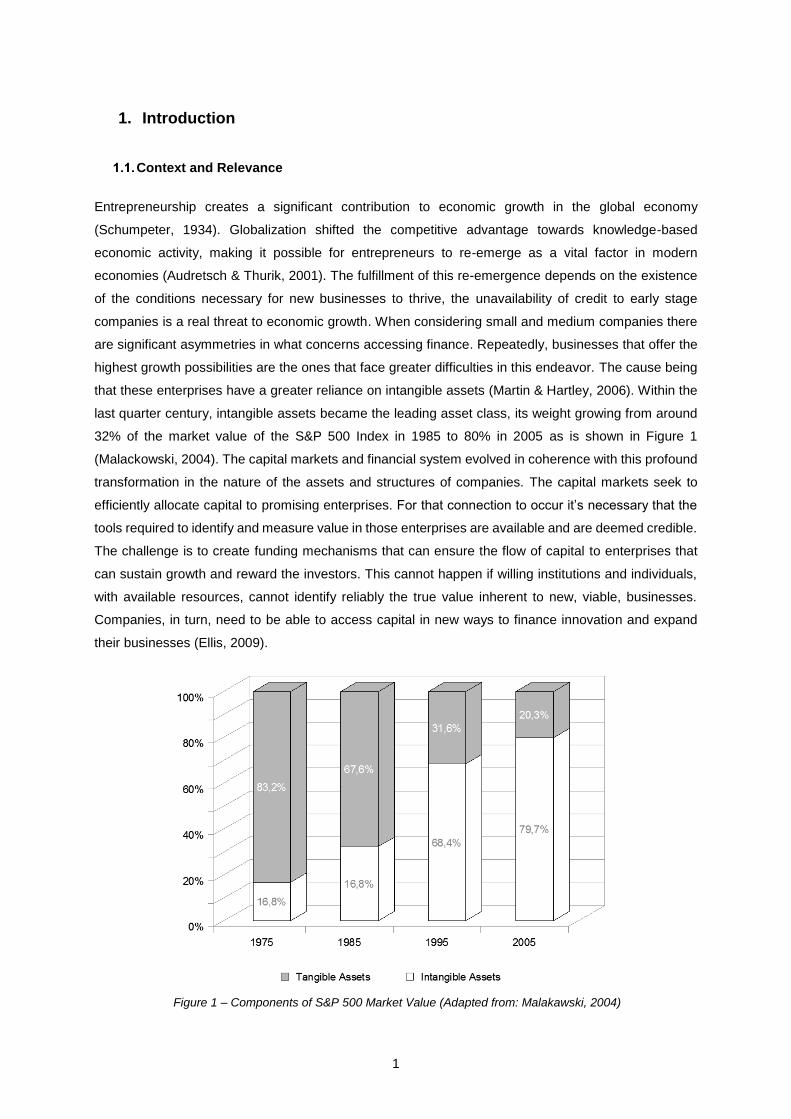
32% of the market value of the S&P 500 Index in 1985 to 80% in 2005 as is shown in Figure 1

(Malackowski, 2004). The capital markets and financial system evolved in coherence with this profound

transformation in the nature of the assets and structures of companies. The capital markets seek to

efficiently allocate capital to promising enterprises. For that connection to occur it’s necessary that the

tools required to identify and measure value in those enterprises are available and are deemed credible.

The challenge is to create funding mechanisms that can ensure the flow of capital to enterprises that

can sustain growth and reward the investors. This cannot happen if willing institutions and individuals,

with available resources, cannot identify reliably the true value inherent to new, viable, businesses.

Companies, in turn, need to be able to access capital in new ways to finance innovation and expand

their businesses (Ellis, 2009).

Figure 1 – Components of S&P 500 Market Value (Adapted from: Malakawski, 2004)

2

The increasing reliance on intangible assets that is particularly relevant in highly technological

companies, creates a lag effect between the development of those assets and the incorporation of its

value in the valuation of the companies. The benefits generated by those assets are only evident when,

directly or not, they result in increased earnings. This has an increased effect in debt financing, due to

the lack of flexibility in the valuation methods that debtors use, effectively reducing the offer of financing

sources that entrepreneurs can access.

Objectives and Motivation

The objective of this work is to study the process of valuation of early stage technological companies

(ESTCs), in a way that provides some guidance not only in regards to their total value but also

considering their capital structure. With this work the author expects to contribute to the literature

associated with the study of the valuation of ESTCs. By incorporating debt in the capital structure and

valuation process, not only a maximization of the value of the company occurs, but also, more

information is created which can be used to justify the access to financing. Instead of developing a

method dedicated to the valuation of the IP, the model that will be developed and tested in this work

valuates the company with regards to the growth of its cash flows, particularly the earnings before

interest and tax (EBIT). The model is grounded on real options analysis (ROA), which enables enough

flexibility for the model to be expanded and adapted not only to companies with different characteristics

but particularly to include investment options such as expansions, acquisitions, delays, among others,

making it useful both for investors and management. Real options analysis also provides adequate

properties to the study of ESTCs by the incorporation of the volatility in the model, which reflects the

uncertainty inherent to the underlying assets on the results of the valuation. Evidence is provided to

support that, for this particular type of company, bank loans are uncommon and difficult to obtain, and

that the use of IP assets to back such loans is a viable, and frequently the only, way to obtain approval.

Providing a model for the valuation of these companies that demonstrates the advantages of debt can

have a positive effect in increasing the offer of financing sources. Investors will be able to benefit from

a more comprehensive valuation of investment projects involving ESTCs. For the field of study of Real

Options Structural Analysis a case study will be added to the available literature with particular properties

that, within the extension of the author’s knowledge upon research, were not yet explored, particularly

the application of a structural model to an ESTC.

3

2. Problem Definition

This work explores the effect of a mixed capital structure, financed by both debt and equity, on the

valuation of ESTCs. A brief review of the methods available to valuate properly registered IP, is made

to indicate the relevance of intangible assets in enabling both debt and equity financing, the setting that

is used in the model. The development and derivation of the model, relying on the existent literature, id

made with enough flexibility to allow for the incorporation of further developments and so that it can be

adapted to the specifications of each venture. An application of the model is then carried out, with the

study of an existing company, Fitbit. The objective of this case study is to validate the use of the model

in the context of ESTCs, also illustrating the challenges in valuating early stage firms and suggesting

solutions for the unavoidable limitations with a critical analysis of the results.

The model makes use of the real options valuation (ROV) framework, to demonstrate the advantages

and possibilities that are enabled by the proper exploration of intangible assets in obtaining debt

financing and thus maximizing the value of the company.

In this work ESTCs are defined as enterprises in a stage of development that is ahead of the end of the

Start-Up Round and the Second Round, or B Series funding; the company in the case study is evaluated

at the moment of the initial public offering (IPO); a more extensive analysis of the development cycle of

ventures is presented in the literature review chapter. It is also assumed that ESTCs are high-growth

capable companies, with most relevant assets being IP assets. A set of companies defined in such a

manner might comprise software, technology, biotechnology or life-sciences companies, among others.

These are the base premises on which Fitbit Inc. was chosen for the practical example, being a

technological company that relies heavily on the ecosystem created by the integration of the hardware

they sell with the digital platform and user interface that accompanies it. Throughout this work, evidence

is quoted and presented that deem this set of characteristics to be an accurate representation of highly

technological startups as a general group.

4

3. Literature Review

The literature review for this project encompasses several different topics and it should provide sufficient

background to justify the decisions made throughout this work as well as provide assistance in its

interpretation.

Investment Cycle and Early Stage Technological Companies

There are multiple definitions of the life cycle associated with the initial stages of companies. Here

follows a description of the early life of a company based on the investment cycle that such companies

undergo. This cycle comprehends six separate phases (Bruno and Tyebjee, 1985), companies may

undergo financing processes in one, several or all of these steps.

Figure 2 – Investment Cycle (Adapted from Wikipedia Commons, 2009)

· Seed-Money Stage – Usually a small amount of capital, it is normally used to prove a concept

or develop a product or prototype.

· Start-Up Funding - Financing for firms in the first years of activity. The application of the funds

is frequently related to marketing and product development costs.

· First-Round Financing – Additional capital to sustain the activity of the company. Firms are

expected to manufacturing and/or sales at this stage.

· Second-Round Financing - Funds used for working capital for companies that are active and

generating revenue but still not making profits.

· Third-Round Financing – Most companies that reach this phase are expected to be breaking-

even. This stage is also called mezzanine financing.

· Fourth-Round Financing – Funding round that antecedes the initial public offering. Also known

as bridge financing.

Each of these rounds of financing involves one or more entities. It is frequent that funders of the first

rounds cannot keep investing in later stages as the monetary amounts and risk levels change

5

considerably along the evolution of the company. For the Seed Stage the most usual sources of

financing are the proverbial three F’s: Family, Friends and Fools. At this stage the risks are usually too

great for institutional funding and the sums involved can the obtained by fundraising from personal

relations.

Business Angels on the other hand tend to intervene in the Start-Up stage or possibly in First-Round

Financing. They are investment professionals who generally invest their own funds. Angel investors are

frequently well-connected, wealthy individuals who can positively influence the results of the enterprise.

The following rounds are usually accomplished by access to venture capital, a professionally managed

pool of capital that is invested in equity-related securities of private ventures at different stages of their

development (Sahlman, 1990). These high risk investments usually seek to generate return through an

eventual realization event, such as an initial public offering (IPO) or a trade sale. The typical venture

capital investments are the First and Second Rounds, also called Series A and B respectively. These

funds frequently have the network to source new highly qualified team members and to enable relations

with flagship customers. Venture Capital investment frequently involves the acquisition of a considerable

percentage of the company’s equity, this transactions are complex and involve more than just the mere

commercialization of property: investors conduct lengthy due diligence, take board seats and secure

rights such as liquidation preferences or tag along, drag along rights. It is common for early investors to

expand their position in the company if it survives to posterior phases. In 2012, venture capital firms

financed 3148 ventures, roughly two thirds of which were follow-up investments into current portfolio

companies (Rockthepost, 2014).

Each business and research area has its own particularities when it comes to relevance of IP, funding

necessities and sources; without discarding such information, the author still finds it appropriate to

extend the scope of this work to what has been defined as the ESTC sector, for the particularities and

scenarios that are used and discussed in this study are deemed to be sufficiently comprehensive.

In addition to what has been defined as the characteristics of ESTCs this work adopts the considerations

of Domodoran (2009) for young companies:

· No history: being recent ventures, young companies have obviously limited data on previous

operations and financials.

· Small or no revenues and operating losses: these companies are still incurring in set-up expenses,

some may not even have started to generate revenues. This usually adds up to substantial operating

losses.

· Dependent on private equity: they are almost entirely dependent on private financing rather than

public markets.

· Many don’t survive: many studies prove that the survival rates of young enterprises are very low.

· Multiple claims on equity: the repeated funding rounds expose first investors to the risk of dilution.

To protect their positions, equity investors often negotiate terms that include first claims on revenues

and liquidation along with control or veto rights.

6

· Investments are illiquid: since the equity is privately held it represents a less liquid asset than that of

publicly traded firms.

Intangible Assets and Intellectual Property

Intangible assets are knowledge-based assets, form part of a company’s intellectual capital, and are

sources of firm-level differentiation and competitive advantage (Martin and Hartley, 2006). Intangible

assets are not usually included in accounting balance sheets (Citron et al., 2004), either because they

do not comply with conventional definitions of assets or because the definition and measuring of their

value falls out of standard accounting practices. They comprise proprietary knowledge, skills and

relationships that form the basis of the uniqueness of each company and, by nature, some of them

cannot easily be acquired in market-based transactions.

The EU Meritum project identifies three distinct categories of intangible assets: ‘human capital’ which

refers to the knowledge and skills of employees; ‘relational capital’, referring to the supply chain,

research and business networks that are available to the firm; and ‘structural capital’, the organizational

competencies of the firm, such as its intellectual property assets.

IP is thusly part of a company’s intangible assets. It refers to creations of the mind: inventions, literary

and artistic works, symbols, names and images used in commerce. Intellectual property is divided into

two categories: Industrial Property includes patents for inventions, trademarks, industrial designs and

geographical indications. Copyright covers literary works, films, music, artistic works and architectural

design (WIPO, n.d.). The key particularity of intellectual property is that it has been granted specific legal

protection and recognition under intellectual property laws.

Figure 3 – Performance of companies with the highest patent scores Versus S&P 500

(Adapted from: Malakawski, 2004)

7

Registering and reporting intangible assets, particularly IP, can provide significant benefits for ESTCs.

The European Union’s 2006 RICARDIS report encouraged policy initiatives to promote the

standardization of the reporting guidelines for research-intensive small and medium enterprises. The

report acknowledges the importance of those policies in the effort to increase the access of those

companies to financing. A start-up firm’s decision to patent is associated with higher annual asset growth

of between 8% and 27%. Also, the decision to patent is associated with substantially improved chances

to survive the first five years of a start-up’s existence (Helmers and Rogers, 2011).

Sources of Finance

Research has shown that the general constraint for financing resides on the supply-side. The lack of

needed capital creates barriers to innovation, condemning young and promising ventures into early

abandonment (Blaug and Lekhi, 2009). From the same source were collected several evidences present

in the literature that support such claims: in a survey of 171 small and medium enterprises from the

United Kingdom, Westhead and Storey (1997) found that for the majority of sample, financial constraints

were a cause for limited investment in innovation and constrained development, with increased

incidence on companies with intensive R%D. A research by Guidici and Paleari (2000), found that 90%

of the surveyed entrepreneurs did not seek debt financing from banks due to a belief that their assets

would be undervalued. In another study, which analyses a sample of 130 technological firms, Ullah and

Taylor (2007) report that almost 80 per cent of firms are finance constrained. Studies with a scope

comprised of companies in the European Union arrived to similar results: Peneder (2008) uses the 2004

European Community Innovation Survey to indicate that small businesses with heavy reliance on

intangible assets are the most susceptible to suffer from insufficient funding.

It is also important to note that informational asymmetries also play a part in perturbing the access to

finance. Investors and other sources of finance have been found to provide inadequate information to

inexperienced entrepreneurs regarding their financial options (Howorth, 2001) with negative

consequences on the trust levels between both parties (Berggren et al, 2000).

This reality makes it necessary to explore and discuss the financing alternatives that are available and

the impacts that they can have in the performance of a company. As this work considers the case of

ESTCs, in which IP assets are of extreme relevance, this review is limited to that scope. Thus the

possible sources of finance are analyzed in a context of IP financing, which is intended as the use of

these intangible assets for raising capital, be it equity or debt. Loans extended on IP assets are a practice

carried out mainly by banks, while venture capitalists and business angels usually provide capital in

return for company shares and are referred to also as private equity. Securitization and leaseback

consist in using IP assets as security to support the borrower’s solvency.

Equity Financing

Equity financing refers to the sale of stake on the ownership of the company, it is intended as a way to

obtain financing for business purposes. In the context of ESTCs, which are privately held companies,

8

this usually translates into the six initial funding rounds, led by venture capital firms, business angels or

crowdfunding.

IP Focused Debt Financing

Debt financing allows companies to raise capital without diluting the equity of the investors. The capital

obtained this way is secured by the assets of the company, in the case of ESTCs this is frequently

restricted to IP assets. Debt also has a fiscal advantage over equity. Intangible asset backed loans

leverage a portfolio of IP or other intangible assets to secure a loan (Ellis, 2009). Companies with the

profile of ESTCs usually face unsurpassable difficulties to obtain debt financing, this is particularly true

since the 2008 credit market crisis (Pavlov, 2009). The uncertainty surrounding intangible asset

valuation also creates barriers for this kind of deals, as it has an essential role in debt financing, firstly

in measuring present and future cash flows for the purpose of servicing the loan repayment, secondly

in assessing the value to cover the investment in case of default (Ellis 2009). Although difficult to obtain,

loans backed by intangibles have been practiced for centuries. The first trade secrets case in the United

States, in 1837, involved debt secured in part by chocolate-making process (Dulken, 2001).

IP Securitizations are a particular form of IP backed debt financing. IP Securitization is a relatively new

procedure, with many national level legal particularities. It is becoming more popular and frequent but,

at the present, the process is still very complex and of difficult access to small and early stage companies

(Tondo-Kramer, 2010). This instrument is used to raise capital as financial security backed by cash

flows such as royalties. In this very complex type of financing, the payments stream from IP assets is

converted into marketable securities placed with investors. The interest models associated with

securitizations can be based on royalties or on an interest over the income, in either case the result for

the company is an anticipation of future earnings. The selling companies are achieving an hedge to the

risk that is implicit in the uncertainty of future cash flow from the revenue; the estimation of the future

viability of the cash flow generating asset is tied to the compensation that the investor demands for

bearing the risk. The creation of devices such as IP auctions has decreased the risk to investors,

allowing more speculative investments, mainly those based on revenue interest securitizations (Jung

and Tamisiea, 2009).

IP Sale and Lease Back

The sale lease-back is a short-term funding strategy that consists in the sale of a portfolio of IP to the

investor, and a contract agreement to license the IP to the selling firm, which allows the utilization of the

assets the activities of the company, in exchange for a fee. Initially the IP owner transfers the ownership

of an IP asset to a leasing company, using the procedures to reinvest in the business. Simultaneously,

a lease of the same asset is made to its former owner, under payment of a loan interest. At the end of

the leasing contract period, the lessee has the option to buy back the ownership of the asset at a fixed

price, by exercising a purchase option (Ellis 2009).

9

IP Valuation

Methods for valuation of IP can be divided in two fundamentally distinct groups: quantitative and

qualitative methods. The latter group is not strictly speaking for valuation, since those methods don’t

output a monetary value. They provide, instead, a value guide based on ratings or scores and are thus

more correctly identified with evaluation than with valuation. Given this explanation, this review will focus

on quantitative methods, which attempt to calculate the monetary value of the IP. There are four

approaches to achieve this purpose: cost approach, market approach, income approach and real

options approach (Mard, 2000; Pavri, 1999, cited in Sudarsanam and Sorwar, 2003).

Cost Approach

Cost based methods are based on the economic principle of substitution, which states that the value of

an asset is equal to the cost incurred in the process of creating an equiparable asset, either internally

or externally. The cost approach can be carried out by measuring the costs in several ways, namely:

· Historic Cost – the costs to be considered are those that were incurred by the company at the time

that the asset was developed.

· Replication Cost – which considers the investment needed to create the same asset at the present

moment, taking into account the entire process of research and development.

· Replacement Cost – the cost of replicating the asset, in its function or utility.

The use of cost based approaches is linked to accounting, as it is the only method of valuation that is in

accordance with accounting principles. In lack of an alternative an incentive is created by the opportunity

to increase awareness towards one’s IP in the financial reports of the company.

Apart from its use in accounting, which in itself is an indicator of the inadequacy of the standard financial

report tools in what concerns IP, there is little advantage in pursuing methods that assume an

equivalence between cost and value. By definition these methods can’t take into consideration future

benefits that can come from the IP, thus creating an unrealistic representation in which an asset that

was costlier to develop is more valuable.

Market Approach

The market approach is straightforward in its definition. The value of the asset is what other actors in

the marketplace deemed it to be. There are multiple methods to establish a market approach valuation:

The price achieved by bidding in a public auction; the market value achieved by a comparable asset in

a previous transaction or the present value of the royalty fees in similar agreements. The pitfall of this

approach is not in its definition or in the results that it produces but in the conditions that it requires to

function, since there is rarely an active market in which are available public information, price and

comparability (AJPark, n.d.).

10

Income Approach

Income based methods measure the potential future benefits of the IP assets and use them to assess

the value of those assets. There are several income based valuation methods: the discounted cash flow

model and others more specific to this category of assets, such as the risk adjusted net present value

or relief from royalty methods.

a. Discounted Cash Flow model

The DCF model is the widespread of the income based valuation approaches. The model outputs the

value of the assets by computing the present value of future cash-flows discounted at a determinate

rate, specific to each market and asset. An extensive description of this method of valuation is presented

in section 3.5.

b. Relief from Royalty method

This method can be related to the “IP Sale and lease back” explained in section 3.3.3. It involves an

assessment of the fee that would have to be payed to license an equivalent IP portfolio from another

source. The royalty represents the fee, which would be paid to the licensor if a hypothetical arrangement

took place. The method assumes that the value of the IP is defined as the royalty other companies

would pay to use it. Estimating this royalty rate is only the first step, a reliable forecast is also required

in order to estimate the direct cash flows from the IP asset. As with other income approaches, the royalty

rates are then discounted through an appropriated discount rate.

As has been previously stated, income approaches are the most commonly used. Despite this fact, they

are also much contested in their ability to produce realistic and fair results. The shortfall of this methods

is the unavoidable uncertainty involved in estimating the future cash flows and overall behavior of the

variables involved. A further limitation is that the individual sources of risk are not necessarily

considered, since the responsibility to incorporate those in the assessment, falls on the analyst and its

interpretation of the discount rate. The advantage of this approach is that, once the required data has

been obtained it is very simple to assess the value of the assets.

Real Options Approach

While not all intangible assets share real option characteristics, many of them are in essence real options

that firms create through their activities, organic investments or acquisitions (Sudarsanam and Marr,

2003). Among these we can consider investments in: human resources, such as education; information

technology; research and development and intellectual property. These investments are rarely

considered as such, we tend to think of them, and accounting defines them, as expenses. But although

they generally don’t generate immediate payoffs, many of them come to produce indirect payoffs and

some even generate direct inbound cash flows. At least these intangibles create the opportunity for

managerial flexibility. When considered as investments it’s of no logic leap to understand that they fit

11

under the characteristics that were defined in the previous chapter for ROA. From this conclusion the

approaches for ROV explored previously apply to the valuation of IP and intangibles in general.

Investment Project Valuation

In this section a review of a traditional valuation model is conducted, the Discounted Cash Flow (DCF)

model, regarding its application to investment projects. Advanced valuation models, particularly those

grounded on real options analysis, are covered in the next section.

Discounted Cash Flow

The DFC model is so embed in the financial world that it has been referred as the heart of most corporate

capital-budgeting systems (Luehrman, 1998).

Net Present Value

This method is based on the net present value (NPV) of the future cash flows (CF) that are expected to

be generated by the investment, which are discounted at an appropriate discount rate (r).

𝑁𝑃𝑉 = ∑𝐶𝐹𝑡

(1 + 𝑟)𝑡

𝑛

𝑡=0

Equation 1 – Net Present Value

At this step predictions of the cash flows are required, for the duration of the investment project. If the

underlying asset for the project is expected to continue to generate cash flows after the end of the

project, an estimate for them can be made and discounted – this is called the Terminal Value. The value

of the underlying asset can be defined as:

𝑉𝑎𝑙𝑢𝑎𝑡𝑖𝑜𝑛 = ∑𝐶𝐹𝑡

(1 + 𝑟)𝑡

𝑛

𝑡=0

+ 𝑇𝑒𝑟𝑚𝑖𝑛𝑎𝑙 𝑉𝑎𝑙𝑢𝑒 Equation 2 – Value of an asset using DCF

Weighted Average Cost of Capital

An appropriate discount rate is required to discount the cash flows. Attention is due to the matching of

the cash flows and the discount rate that is used, this being especially relevant when valuing companies.

An example that arises frequently is the consideration between CFs to the firm and CFs to the equity,

with the consequence of considering a discount rate that has implied the cost of capital associated with

the entire capital structure or one that only considers equity. The weighted average cost of capital

(WACC) is the most widely accepted discount rate (Pratt and Grabowski, 2014).

12

Cost of Equity

The cost of equity (𝑟𝑒) is calculated with the use of the capital asset pricing model (CAPM). This model

represents the return rate that investors require from the investment, which should be interpreted as the

combination of two factors: the compensation of time and risk.

According to the CAPM, the cost of equity can be estimated as:

𝑟𝑒 = 𝑟𝑓 + (𝑟𝑚 − 𝑟𝑓)𝛽 Equation 4 – Cost of Equity

𝑟𝑓 – risk free rate; rm – market return

The risk free rate (𝑟𝑓) is the rate of return associated with an investment were the actual return is equal

to the expected return, it is a measure of the time value of capital, which implies no variance around the

expected return (Domodaran, 2012). According to the same source the rate of a government bond (in

the same currency as the investment) provides a good approximation of a true risk free rate. It is also

referred that while a long term bond is a good standard there should be some correspondence between

the duration of the investment and the maturity of the bond.

The market risk premium (𝑟𝑚 − 𝑟𝑓) is the reward required by investors to bear the average risk of

investing in the market discounted of the risk free rate. Definition requires it to be greater than zero,

increase with the risk aversion of the investors in that market and increase with the average risk in that

market (Domodaran, 2012). The standard approach to calculate this premium is to use historical data:

define a time period for the estimation; calculate average returns on a stock index during that period

(𝑟𝑚); calculate the difference between that rate and the risk free rate.

The variable beta (𝛽) is the risk that holding the security will add to the investor’s portfolio (Rhaiem et

al, 2007). It is most frequently derived using linear regression analysis, where the return of the security

(𝑟𝑠𝑒𝑐𝑢𝑟𝑖𝑡𝑦) is the dependent variable and the market return (𝑟𝑚) is the independent variable. The beta is

the slope of the regression line.

𝛽 = 𝐶𝑜𝑣(𝑟𝑠𝑒𝑐𝑢𝑟𝑖𝑡𝑦 , 𝑟𝑚)

𝑉𝑎𝑟(𝑟𝑚) Equation 5 – Beta

This empirical determined input variable is also dependent on the company’s historical level of leverage,

because higher leverage ratios increase the shareholder’s risk. Considering that a company’s level of

𝑊𝐴𝐶𝐶 = 𝐸

𝑉𝑟𝑒 +

𝐷

𝑉𝑟𝑑(1 − 𝑡)

Equation 3 – Weighted Average Cost of Capital

E – Equity Value; D- Debt; V – Enterprise Value = E + D;

𝑟𝑒 – cost of equity; 𝑟𝑑 – unadjusted cost of debt; t – tax rate

13

leverage can change considerably during a transaction, the beta might have to be adjusted for this

change by unlevering and relevering to the new capital structure (Steiger, 2008).

With non-listed companies there isn’t available data to compute the linear regression. For such cases,

Damodaran (2012) offers a way to compute an accounting beta: estimating it by regressing the changes

in the earnings of the firm against the same variations measured from a market index.

∆ 𝐸𝑎𝑟𝑛𝑖𝑛𝑔𝑠𝑐𝑜𝑚𝑝𝑎𝑛𝑦 = 𝑎 + 𝑏 ∗ ∆ 𝐸𝑎𝑟𝑛𝑖𝑛𝑔𝑠𝑚𝑎𝑟𝑘𝑒𝑡 Equation 6 – Procedure for Accounting Beta

The lack of accounting data, measured with much less frequency than the prices of a market traded

asset, limits the quality of this estimates (Damodaran, 2012). This limitation is increased for early stage

companies, where accounting information is restricted to the short life of the firm.

Cost of Debt

The cost of debt (𝑟𝑑(1 − 𝑡)) is the interest rate that the market demands for the debt sold (Steiger, 2008).

The author identifies three variables that influence the cost of debt: the base interest rates in the market,

which reflect on the risk free rate; the default premium and the firm's effective tax rate. The cost of debt

does not correspond to the interest rate that the company pays for the debt that it has inscribed on its

books (Damodaran, 2012).

If the firm has currently traded bonds outstanding, the yield to maturity on a long-term bond can be used

as the interest rate. Otherwise, if the company is rated by a credible entity that rating can be used to

estimate a default spread. For companies that don’t fulfill this requirements, two possible approaches

are: using the interest rate from a recent long term bank loan or to estimate a synthetic rating to obtain

a spread. In its simplest form, the rating can be estimated from the interest coverage ratio:

𝐼𝑛𝑡𝑒𝑟𝑒𝑠𝑡 𝐶𝑜𝑣𝑒𝑟𝑎𝑔𝑒 𝑅𝑎𝑡𝑖𝑜 = 𝐸𝐵𝐼𝑇

𝐼𝑛𝑡𝑒𝑟𝑒𝑠𝑡 𝐸𝑥𝑝𝑒𝑛𝑠𝑒𝑠 Equation 7 – Interest Coverage Ratio

To calculate the equity and debt weights ( 𝐸

𝑉 𝑎𝑛𝑑

𝐷

𝑉 ) market values should be used. Since debt and

equity are traded at market values, and the cost of capital is a measure of the cost of raising the

necessary finance to conclude the investment, the WACC is better estimated using market weights

(Damodaran, 2012).

Real Option Analysis

Methods like the DCF model fail to consider the options that are embedded in such actions as a decision

to invest, or in making capital structure decisions. The net present value of a project, calculated with the

DCF method, cannot incorporate the implied value of the options to delay, expand or abandon a project

14

(Damodaran, 2012). It also lacks a proper way to deal with uncertainty, and the measurement of the

risk, represented by the β coefficient, is of limited application for assets that are not publicly traded. The

same source warns of a lack of unanimity among theorists and practitioners for the way in which to use

ROA: “some view it as a rhetorical tool that can be used to justify investment, financing and acquisition

decisions” but do not recognize the capability to valuate those options with any precision. There are

others who argue that quantitative estimation of the value of these options should be used, and built into

the decision process.

An option can be defined generally as a right but not an obligation, at or before some specified time, to

purchase or sell an underlying asset whose price is subject to some form of random variation. Most

obviously though the underlying asset can be a share in a company whose price varies over time as a

form of random walk variation (Pitkethly 1997).

First an introduction to the basic concepts of options and option pricing, following Domodaran

(Domodaran, 2012). There are two types of options:

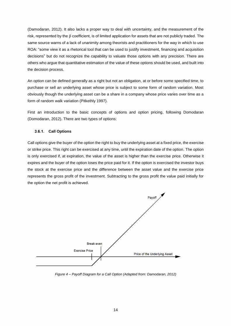
Call Options

Call options give the buyer of the option the right to buy the underlying asset at a fixed price, the exercise

or strike price. This right can be exercised at any time, until the expiration date of the option. The option

is only exercised if, at expiration, the value of the asset is higher than the exercise price. Otherwise it

expires and the buyer of the option loses the price paid for it. If the option is exercised the investor buys

the stock at the exercise price and the difference between the asset value and the exercise price

represents the gross profit of the investment. Subtracting to the gross profit the value paid initially for

the option the net profit is achieved.

Figure 4 – Payoff Diagram for a Call Option (Adapted from: Damodaran, 2012)

15

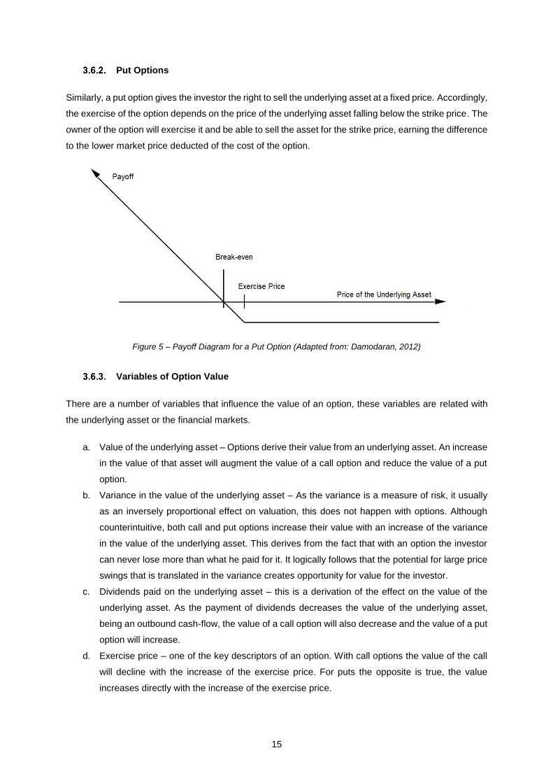
Put Options

Similarly, a put option gives the investor the right to sell the underlying asset at a fixed price. Accordingly,

the exercise of the option depends on the price of the underlying asset falling below the strike price. The

owner of the option will exercise it and be able to sell the asset for the strike price, earning the difference

to the lower market price deducted of the cost of the option.

Variables of Option Value

There are a number of variables that influence the value of an option, these variables are related with

the underlying asset or the financial markets.

a. Value of the underlying asset – Options derive their value from an underlying asset. An increase

in the value of that asset will augment the value of a call option and reduce the value of a put

option.

b. Variance in the value of the underlying asset – As the variance is a measure of risk, it usually

as an inversely proportional effect on valuation, this does not happen with options. Although

counterintuitive, both call and put options increase their value with an increase of the variance

in the value of the underlying asset. This derives from the fact that with an option the investor

can never lose more than what he paid for it. It logically follows that the potential for large price

swings that is translated in the variance creates opportunity for value for the investor.

c. Dividends paid on the underlying asset – this is a derivation of the effect on the value of the

underlying asset. As the payment of dividends decreases the value of the underlying asset,

being an outbound cash-flow, the value of a call option will also decrease and the value of a put

option will increase.

d. Exercise price – one of the key descriptors of an option. With call options the value of the call

will decline with the increase of the exercise price. For puts the opposite is true, the value

increases directly with the increase of the exercise price.

Figure 5 – Payoff Diagram for a Put Option (Adapted from: Damodaran, 2012)

16

e. Time to expiration – the effect is similar to what was said about the variance in the value of the

underlying asset. Longer times create more opportunity for the price of the underlying asset to

change, as the losses are limited to the price paid for the option, this increases the value of

options, either calls or puts.

f. Risk free rate – this factor interacts with the value of an option in two different ways. Firstly, as

the investor pays up front for the option, there is an opportunity cost which will depend on the

market interest rates and time to expiration of the option. Secondly, the risk free rate takes part

in the valuation of the option in the computation of the present value of the exercise price. A

positive variation of the risk free rate originates an increase in the value of a call option and a

decrease on the value of a put option.

American and European Options

Options are classified as American or European according to the possibility to exercise them at times

prior to their expiration. American options can be exercised at any moment prior to that date, European

options can only be exercised at expiration. The enhanced flexibility that this property confers to the

American options makes them more valuable but also increases the difficulty of their valuation. In

practical terms this is rarely a limitation as the models for European options can be applied to American

options as long as the execution only takes place at expiration. Exercising the option early is frequently

undesirable due to the time premium, which is expected to decrease as the expiration nears, and the

transaction costs. This means that selling the option is usually preferable to exercising it before the

expiration date. A relevant exception is the case where the underlying asset pays large dividends,

causing the value of the asset to decrease, with negative impact on call options associated with it.

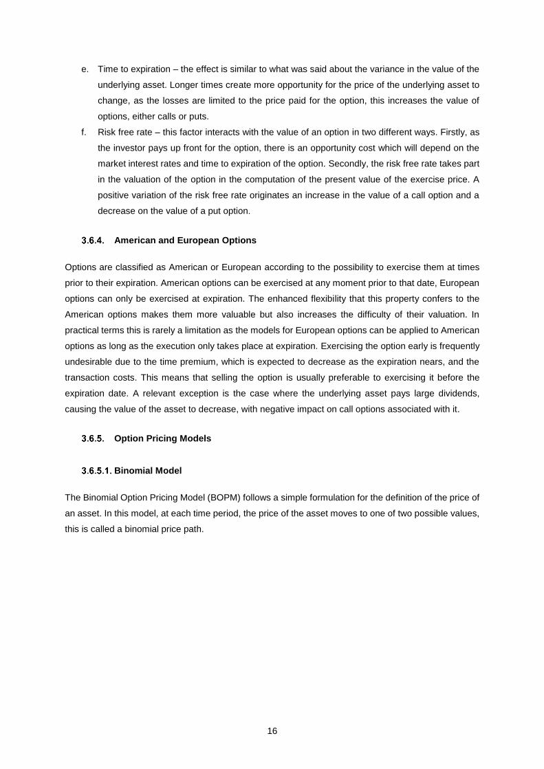
Option Pricing Models

Binomial Model

The Binomial Option Pricing Model (BOPM) follows a simple formulation for the definition of the price of

an asset. In this model, at each time period, the price of the asset moves to one of two possible values,

this is called a binomial price path.

17

The BOPM is a discrete-time model for asset price movements, which follows a time interval (t) between

price movements.

The valuation in a binomial process is done iteratively, starting from the last time period and following

back in time until the starting point. After each interval an option replicating portfolio is created and

evaluated, by the principles of arbitrage the value of the replicating portfolio is equal to the value of the

option. The replicating portfolio is a combination of risk-free borrowing or lending and a number of units

of the underlying asset, it aims to reproduce the same cash flows as the option being valued. The

number of units of the underlying asset is called the option delta (∆) and is defined, at each time step,

as:

∆ = 𝐶𝑢 − 𝐶𝑑

𝑆𝑢 − 𝑆𝑑 Equation 8 – Option Delta

The binomial option pricing model outputs the composition of the replicating portfolio, which gives us

the value of a call option, defined as:

𝐶 = 𝑆∆ − 𝐵

Equation 9 – Value of a Call using the BOPM

C – Value of the call; S – Current value of the asset;

∆ – Option delta; B – Borrowing necessary to replicate the option

Stochastic Differential Equations

Analytical models for option pricing are based on the assumption that the state variable depends on

underlying random processes and is represented by a stochastic differential equation (SDE). Brownian

p

1-p

Figure 6 – Binomial Lattice (Adapted from: Brandão, 2005)

18

motion is one of the possible random processes that drive SDEs. This continuous time process is

frequently called Wiener process, both denominations being interchangeable (Wiersema, 2008).

One SDE, using one Brownian motion as the source of motion is the arithmetic Brownian motion (ABM)

or standard Brownian motion. The equation has the form:

𝑑𝑥(𝑡) = µ𝑑𝑡 + 𝜎𝑑𝑊

Equation 10 – Arithmetic Brownian Motion

𝑥 – state variable; µ – drift (constant); 𝑡 – time;

𝜎 – standard deviation (constant); 𝑊 – Wiener

process ; 𝑑 – mathematical differential operator

The coefficient 𝜎 is a scaling factor of the random process created by the Brownian motion. The other

term, µ, is the drift, it determines the non-random component of the evolution of the variable. In the

equation, µ and 𝜎 are known constants and 𝜎 > 0. The random variable 𝑥(𝑡) is normally distributed, with

the distribution parameters 𝐸(𝑥(𝑡)) = 𝑥0 + 𝜇𝑡 and 𝑉𝑎𝑟(𝑥(𝑡)) = 𝜎2𝑡. As this model attributes a normal

distribution to the variable 𝑥(𝑡), it can take negative values. For this reason it has been discarded in the

modelling of stock prices, which are prevented from becoming negative because of the limited liability

enjoyed by equity owners. The capability of reaching negative values can be extremely useful when the

variable is not the price of a stock, but an underlying financial measure, such as earning.

The SDE that as traditionally been used to model stock prices is the Geometric Brownian motion (GBM).

This model is represented by Equation 11, with similarities to that of the ABM (Wiersema, 2008),

substituting the variable 𝑥(𝑡) by the rate of change of the same variable 𝑑𝑥(𝑡)

𝑥(𝑡).

𝑑𝑥(𝑡) = x(t)µ𝑑𝑡 + x(t)𝜎𝑑𝑊 Equation 11 – Geometric Brownian Motion

The parameters 𝜇 and 𝜎 are constants as in the ABM. Under this model the variable follows a lognormal

distribution, which does not allow negative values. The drift and random coefficients, respectively x(t)µ

and x(t)𝜎, are always proportional to the current value of the variable x(t), which amounts to exponential

growth. The parameters of the lognormal distribution are 𝐸(𝑥(𝑡)) = 𝑥0𝑒𝜇𝑡 and 𝑉𝑎𝑟(𝑥(𝑡)) =

𝑥02𝑒2𝜇𝑡(𝑒𝑡𝜎2

− 1).

Black-Scholes Model

The Black Scholes Option Pricing Model (BSOPM) is one of the most outstanding models in financial

economics (Sudarsanam and Sorwar, 2003).

19

Although the model is rarely mentioned as Black-Scholes-Merton model, the contribution of Robert

Merton to the field was considered sufficiently relevant by the Swedish Academy to be awarded with the

1997 Nobel Prize in Economics, shared with Scholes.

The BSOPM is a limiting case of the binomial pricing model. As the time interval tends to zero, the

limiting distribution tends to one of two forms: a normal distribution, if price changes reduce as the time

interval is shortened, in which case the price function becomes continuous; or a Poisson distribution if

price jumps are to be allowed. The BSOPM corresponds to the case when the limiting distribution is

normal.

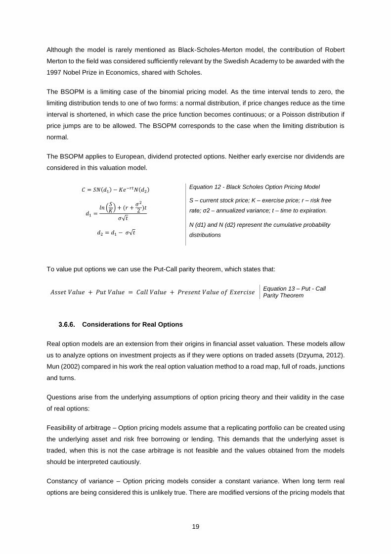
The BSOPM applies to European, dividend protected options. Neither early exercise nor dividends are

considered in this valuation model.

𝐶 = 𝑆𝑁(𝑑1) − 𝐾𝑒−𝑟𝑡𝑁(𝑑2)

𝑑1 =𝑙𝑛 (

𝑆𝐾

) + (𝑟 +𝜎2

2)𝑡

𝜎√𝑡

𝑑2 = 𝑑1 − 𝜎√𝑡

Equation 12 - Black Scholes Option Pricing Model

S – current stock price; K – exercise price; r – risk free

rate; σ2 – annualized variance; t – time to expiration.

N (d1) and N (d2) represent the cumulative probability

distributions

To value put options we can use the Put-Call parity theorem, which states that:

𝐴𝑠𝑠𝑒𝑡 𝑉𝑎𝑙𝑢𝑒 + 𝑃𝑢𝑡 𝑉𝑎𝑙𝑢𝑒 = 𝐶𝑎𝑙𝑙 𝑉𝑎𝑙𝑢𝑒 + 𝑃𝑟𝑒𝑠𝑒𝑛𝑡 𝑉𝑎𝑙𝑢𝑒 𝑜𝑓 𝐸𝑥𝑒𝑟𝑐𝑖𝑠𝑒 Equation 13 – Put - Call Parity Theorem

Considerations for Real Options

Real option models are an extension from their origins in financial asset valuation. These models allow

us to analyze options on investment projects as if they were options on traded assets (Dzyuma, 2012).

Mun (2002) compared in his work the real option valuation method to a road map, full of roads, junctions

and turns.

Questions arise from the underlying assumptions of option pricing theory and their validity in the case

of real options:

Feasibility of arbitrage – Option pricing models assume that a replicating portfolio can be created using

the underlying asset and risk free borrowing or lending. This demands that the underlying asset is

traded, when this is not the case arbitrage is not feasible and the values obtained from the models

should be interpreted cautiously.

Constancy of variance – Option pricing models consider a constant variance. When long term real

options are being considered this is unlikely true. There are modified versions of the pricing models that

20

allow for changing variances as long as the process by which the variance changes can be modeled

explicitly (Domodaran, 2012).

Instantaneous exercise - The exercise of most real options takes time, this implies that the true life of a

real option is often less than the stated life.

Investment Opportunities as Real Options

Real Options turn a limited commitment into future decision rights (McGrath et al. (2004). The increased

flexibility for management decisions and potential future benefits that they enable can, sometimes, lead

to the viability of the analyzed project, even if classical NPV analysis yields negative returns.

The real option valuation method lets us evaluate multiple aspects of an investment project that would

be neglected with a traditional investment analysis. Some of those options are:

a. Option to abandon

The option to abandon a project only makes sense when we’re considering a multi-stage or repeated

investment project. In such conditions, if at any moment in time the value of liquidating the project is

greater than the remaining value of the project, than it should be liquidated. This analysis is based on

the assumption that the liquidation or residual value is constant during the life of the project. The opposite

would probably have more realistic application but the use of standard option pricing models wouldn’t

be adequate. The payoff graph associated with an option to abandon is similar to that of a put, and the

option fits that category.

b. Option to delay

It is the most basic condition for the viability of a project that the net present value of its expected cash

flows is positive. However, by changes in the underlying conditions or merely on the basis for the

estimations, the expected cash flows and the discount rates may change over time, altering the NPV.

This means that the viability and the expected return of a project may change by the mere action of a

delay. The characteristics of this kind of option are consistent with those of an American call option. It is

advisable to take into consideration that the option to delay might create opportunity for other players in

a competitive market.

c. Option to expand

Some projects cannot be assessed just by themselves. Consider the case in which the decision to

execute a project enables, in a known timeframe, other projects. This is an option to expand a project.

Even if the first part of the project has a negative NPV, the valuation of the option to expand can be

enough to offset the returns and make the project viable. It is correct to consider this option as a call, at

the end of the timeframe to expand, the investor will enter the second phase of the project if the NPV at

that time has turned positive. While this rationale may be used to justify initial investments that do not

21

meet the financial requirements in a standard analysis, not all of these investments create valuable

options. The value of the option comes from the capability of generating increased returns that is

enabled by the strategic action that is associated with it.

d. Other options

Portfolios constituted by a combination of the above can be constructed to simulate such real options

as a switch (e.g. the abandonment of a technology for another) or a staged growth, among others

(Dzyuma, 2012).

Structural Models

Structural models are based on the assumption that the dynamics of the project variable are described

by a stochastic differential equation. From that assumption, it is possible to find the present values of

different claims, such as debt, equity and taxes through the solution of a partial differential equation.

This pricing framework is based on the work of Black and Scholes (1973) and Merton (1974). If

differentiating conditions between debt and equity are incorporated, such as the tax advantage of debt,

it is possible to derive the optimal coupon level which maximizes the firm value, thus defining the optimal

capital structure. Most structural models, particularly early ones, share some core characteristics: the

project variable is the value of the firm’s assets, which is assumed to have dynamics described by a

geometric Brownian motion (GBM) and they have a static setting, meaning that debt can be issued only

once. The works of Brennan and Schwartz (1978) and Leland (1994) belong to that family of models.

Dynamic capital structure models were first introduced by Kane, Marcus, and McDonald (1984). Later

contributors include Fischer et al. (1989) and Goldstein et al. (2001). The first generation of structural

models suffers from a particular inconsistency (Ammann and Genser, 2004): the state variable of the

models is the unlevered firm value. This implies that both the levered and unlevered value of the firm

exist simultaneously, which is not viable in an asset pricing context. Goldstein et al. (2001) proposed a

model that uses an income measure that is unaffected by the capital structure decision, the EBIT. This

type of model is more consistent with regular practices because debt coupons are financed with

earnings, not by issuing new equity. The model divides the present value of the EBIT between several

claims.

Ammann and Genser (2004) propose a model which features an alternative assumption for the

dynamics of the project variable: instead of the commonly assumed GBM they opt for an arithmetic

Brownian motion (ABM). Few other works use ABM as the underlying process, among them are Bank

and Lawrenz (2005), and Genser (2006). These models are all in a static setting, although the works of

Ammann and Genser (2004) and Genser (2006) do allow for debt with finite maturities.

The use of geometric Brownian motion in all dynamic structural models, so far, is due to the fact that its

mathematical properties allow a simplified progression from the static setup to the dynamic one, which

is due to a homogeneity property inherent to this particular stochastic process. Since most start-ups do

22

exhibit negative operating income, the assumption of GBM would be fairly limiting from a practical angle

(Alexander et al., 2012).

23

4. Methodology

This chapter covers the definition, justification and development of the model. Using an approach

grounded on structural analysis makes it possible to define the optimal capital structure as well as the

value of the company and option to invest. By modelling EBIT growth as an ABM, instead of the more

frequent assumption of GBM, it becomes possible to incorporate the possibility of negative cash flows,

thus making the model more adapted to the reality of ESTCs. The use of debt as well as equity, reaching

the optimal capital structure, enables the management of the firm to maximize the value of the company

through the tax benefits of debt.

This model is developed within a static capital structure framework. In this setting the optimal leverage

is evaluated for a particular EBIT level, without the option of additional issuances of debt in the future.

Dynamic optimal leverage has been studied by Fischer et al. (1989), Goldstein et al. (2001), among

others. All these works share the underlying assumption that the state variable follows a GBM. To the

extent of the author’s knowledge, so far, no researcher has published work concerning an ABM based

dynamic capital structure model.

A static model can provide not only information on the current capital structure, but also on how far the

current leverage is from the optimal one. Used as a reference it provides guidance but maintains

management flexibility and adaptability to different scenarios.

Main assumptions of the valuation model

The choice of the project variable and of the stochastic differential equation that governs its dynamics

is a fundamental step of the development of the model. While it can´t be categorically stated that the

decisions made in this work represent a solution compatible with all cases, it is possible to present

justifications and reasoning to make the case that they provide the better fit for the characteristics

inherent to ESTCs. It is also relevant to try to understand why the majority of the literature opts for a

different approach, particularly in what concerns the GBM assumption. As was mentioned in section 3.6,

the researchers that started the study of structural models, were heavily influenced by the BSOPM and

other asset pricing models developed for market traded assets with the market price as state variable,

which demanded that the modelling of such variables did not allow negative values, which is warranted

by the use of the GBM.

Earnings Before Interest & Tax (EBIT): The project variable

The majority of the real options based models fit into one of two categories, in what concerns the project

variables: those that model the value of the firm or of the equity, and the ones that model some form of

cash flows. The more traditional approach, of modelling firm or equity value, carries some disadvantages

that make it unsuitable for this project. One of the difficulties with these models is the definition of the

tax benefits, which are treated has inflows of capital, rather than a reduction of the outflow of taxes. Not

only is this conceptually wrong, it leads to severe problems in the behavior of such models. Comparative

24

statics analysis shows that this assumption causes the present value of the equity to increase with the

tax rate (Goldstein et al, 2001).

The researchers that opted for the use of cash flows as project variables used either EBIT, Free Cash

Flow or Revenue. This work uses EBIT, which is the most frequent decision among this class of models.

Ammann and Genser (2004) argue that the most important advantage of choosing this project variable

is the fact that working with EBIT and DCF based models allows for the cash flows to be split into

different claims. Goldstein et al (2001) corroborates: “The implication is that all contingent claimants

(equity, debt, government, etc.) to future EBIT flows are treated in a consistent fashion.” Other strength

of this approach is considering that existing claims to future EBIT are mostly insensitive to changes in

capital structure. It is standard practice to assume that the EBIT-generating activities of a firm, are

independent from capital structure (Modigliani and Miller, 1958; Merton, 1974; Brennan and Schwartz,

1978).

Throughout this work the use of EBIT and Operating Income (OI) will be made without distinguishing

between the two. There are differences between the two, but those mainly regard adjustments in special

items. The OI is the measure recommended in the generally accepted accounting principles (GAAP). In

the context of this academic exercise in company valuation, and more broadly in financial analysis both

concepts can be considered equivalent and defined as the revenue subtracted of the operating

expenses.

Arithmetic Brownian Motion: Modelling Earnings Before Interest & Tax

Assuming that the market prices of financial derivatives on market-traded assets follow a GBM is a

standard assumption (Brandão et al., 2005). A frequent argument favoring GBM is that prices modelled

this way do not become negative, a condition that also holds for market traded assets.

The stochastic process that is used to model and simulate the EBIT flows is essential to the model.

When dealing with cash flows, which are not market traded assets, they can, and frequently do, become

negative. Recognizing this, Copeland and Antikarov (2001), suggest that sometimes ‘‘it may be better

to model the value of the underlying as an arithmetic or additive process’’.

Here an ABM process is used, in substitution of the most common GBM assumption. Although

uncommon this option is not unique and was taken, for purposes similar to those of this work, by

Ammann and Genser (2004), Genser (2005) and Bank and Wibmer (2012); as well as for pricing credit

spread options (Giacometti and Teocchi, 2005) and valuing real options, Alexander et al (2012).

The most relevant reason not to use GBM in this project is the fact that the implied log-normal

distribution of the project variable values, excludes negative ranges (Alexander et al, 2012). This

limitation is particularly relevant when one is assessing the cash flows of young firms or trying to evaluate

the possible outcomes of a future venture. In the case of ESTCs it’s frequently verified that the

companies operate with negative EBIT.

25

Development of a Structural Model

Having justified the choice of EBIT as the project variable and of ABM as stochastic process, the

construction of the model can be carried out. The following process follows analogous steps to those

present in the works of Goldstein et al (2001), Ammann and Genser (2004), Genser (2006) and Bank

and Wibmer (2012). These and other authors will be referred in particular settings, when necessary to

justify decisions or unobvious steps. The structural model computes the present value of the EBIT

generated by the company, as estimated by the dynamics of the ABM; then it distributes that total value

among the different claimants: in an unlevered setting the division is between the equity owners, the

state, which is entitled to taxes, and to closure costs, associated with the abandonment of business if

the EBIT falls below a threshold value, the optimal threshold is also evaluated. In a levered setting,

besides the already stated claims, there is also a debt claim and one related with the costs of bankruptcy,

conditions for which are also estimated in the model. The maximization of the value of the company is

achieved because of the tax advantage to debt, this makes it possible to compute an optimal capital

structure for the company in the conditions of the valuation model. The value of the company is

considered to be the present value of the claims to equity, net of taxes and closure costs, in the

unlevered case and to the sum of equity and debt in the levered company.

Value of a claim to cash flows following ABM

The starting point of the model is the stochastic differential equation of the ABM process:

𝑑𝑥(𝑡) = µ𝑑𝑡 + 𝜎𝑑𝑊

Equation 14 – Arithmetic Brownian Motion (repeated)

𝑥 – state variable; µ – drift (constant); 𝑡 – time;

𝜎 – standard deviation (constant); 𝑊 – Wiener

process ; 𝑑 – mathematical differential operator

Discounting the expected cash flows under the risk-neutral measure gives the pricing of the subjacent

asset (Goldstein et al., 2001). The expected present value of the EBIT flow is:

𝑉𝑒𝑥𝑝𝑒𝑐𝑡𝑒𝑑(𝑥) = 𝐸𝑄 [∫ 𝑥𝑒−𝑟𝑡+∞

𝑡

𝑑𝑡] = µ

𝑟2+

𝑥

𝑟

Equation 15 – Expected Present Value of the EBIT

𝐸 – expected value operator; 𝑟 – risk free rate

Assuming that no arbitration is possible, defining a risk-neutral measure, Q, guarantees that every claim

will receive the expected return for the assumed risk. With µ = µ𝑚 − σΦ being the risk neutral drift, µ𝑚

the measured drift and Φ the risk premium.

The ABM process being an Itô’s process, it is possible to affirm, according to Itô’s Lemma, that any

perpetual claim to 𝑉(𝑥) must follow dynamics such as:

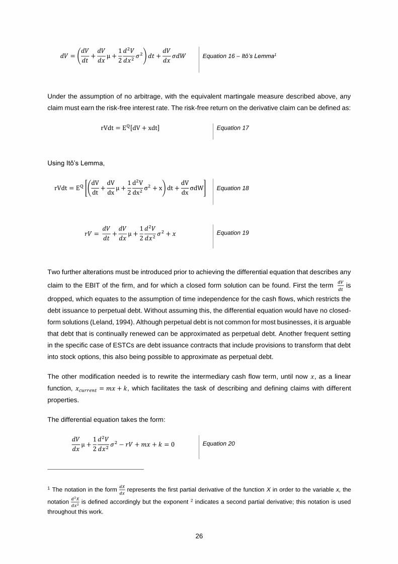
26

𝑑𝑉 = (𝑑𝑉

𝑑𝑡+

𝑑𝑉

𝑑𝑥µ +

1

2

𝑑2𝑉

𝑑𝑥2𝜎2) 𝑑𝑡 +

𝑑𝑉

𝑑𝑥𝜎𝑑𝑊 Equation 16 – Itô’s Lemma1

Under the assumption of no arbitrage, with the equivalent martingale measure described above, any

claim must earn the risk-free interest rate. The risk-free return on the derivative claim can be defined as:

rVdt = EQ[dV + xdt] Equation 17

Using Itô’s Lemma,

rVdt = EQ [(dV

dt+

dV

dxµ +

1

2

d2V

dx2σ2 + x) dt +

dV

dxσdW] Equation 18

𝑟𝑉 = 𝑑𝑉

𝑑𝑡+

𝑑𝑉

𝑑𝑥µ +

1

2

𝑑2𝑉

𝑑𝑥2𝜎2 + 𝑥 Equation 19

Two further alterations must be introduced prior to achieving the differential equation that describes any

claim to the EBIT of the firm, and for which a closed form solution can be found. First the term 𝑑𝑉

𝑑𝑡 is

dropped, which equates to the assumption of time independence for the cash flows, which restricts the

debt issuance to perpetual debt. Without assuming this, the differential equation would have no closed-

form solutions (Leland, 1994). Although perpetual debt is not common for most businesses, it is arguable

that debt that is continually renewed can be approximated as perpetual debt. Another frequent setting

in the specific case of ESTCs are debt issuance contracts that include provisions to transform that debt

into stock options, this also being possible to approximate as perpetual debt.

The other modification needed is to rewrite the intermediary cash flow term, until now 𝑥, as a linear

function, 𝑥𝑐𝑢𝑟𝑟𝑒𝑛𝑡 = 𝑚𝑥 + 𝑘, which facilitates the task of describing and defining claims with different

properties.

The differential equation takes the form:

𝑑𝑉

𝑑𝑥µ +

1

2

𝑑2𝑉

𝑑𝑥2𝜎2 − 𝑟𝑉 + 𝑚𝑥 + 𝑘 = 0 Equation 20

1 The notation in the form 𝑑𝑋

𝑑𝑥 represents the first partial derivative of the function X in order to the variable x, the

notation 𝑑2𝑋

𝑑𝑥2 is defined accordingly but the exponent 2 indicates a second partial derivative; this notation is used

throughout this work.

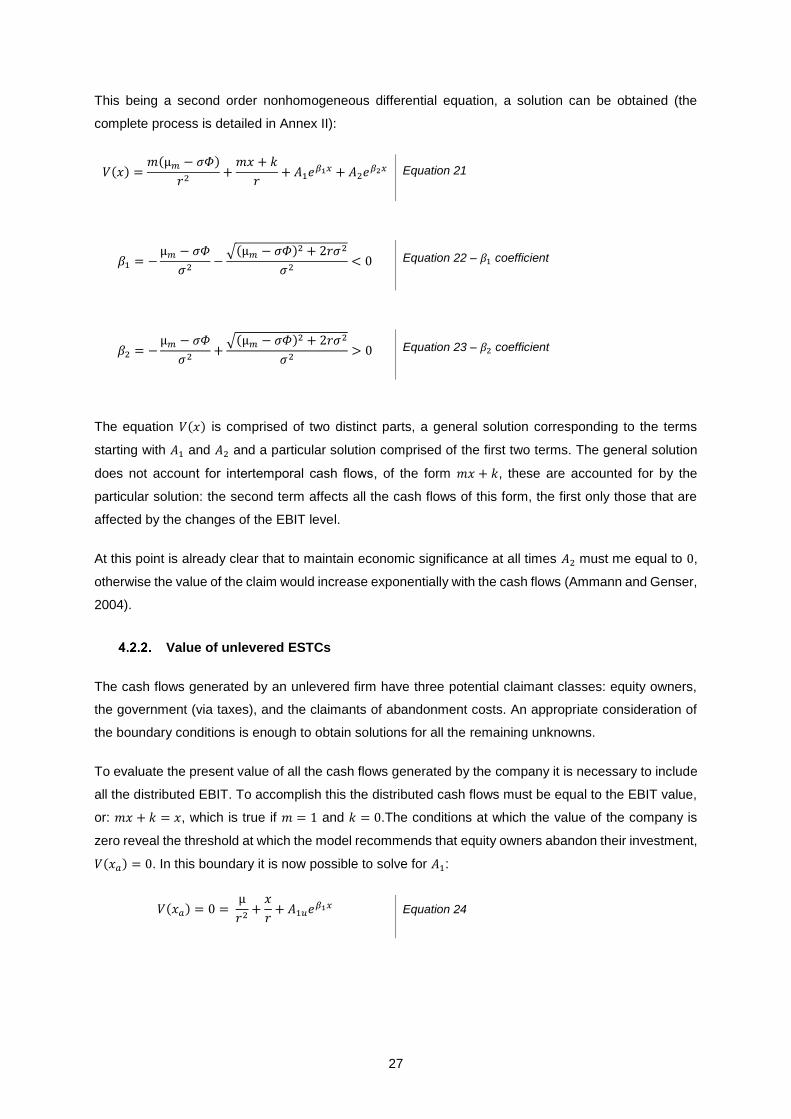
27

This being a second order nonhomogeneous differential equation, a solution can be obtained (the

complete process is detailed in Annex II):

𝑉(𝑥) =𝑚(µ𝑚 − 𝜎𝛷)

𝑟2+

𝑚𝑥 + 𝑘

𝑟+ 𝐴1𝑒𝛽1𝑥 + 𝐴2𝑒𝛽2𝑥 Equation 21

𝛽1 = −µ𝑚 − 𝜎𝛷

𝜎2−

√(µ𝑚 − 𝜎𝛷)2 + 2𝑟𝜎2

𝜎2< 0 Equation 22 – 𝛽1 coefficient

𝛽2 = −µ𝑚 − 𝜎𝛷

𝜎2+

√(µ𝑚 − 𝜎𝛷)2 + 2𝑟𝜎2

𝜎2> 0 Equation 23 – 𝛽2 coefficient

The equation 𝑉(𝑥) is comprised of two distinct parts, a general solution corresponding to the terms

starting with 𝐴1 and 𝐴2 and a particular solution comprised of the first two terms. The general solution

does not account for intertemporal cash flows, of the form 𝑚𝑥 + 𝑘, these are accounted for by the

particular solution: the second term affects all the cash flows of this form, the first only those that are

affected by the changes of the EBIT level.

At this point is already clear that to maintain economic significance at all times 𝐴2 must me equal to 0,

otherwise the value of the claim would increase exponentially with the cash flows (Ammann and Genser,

2004).

Value of unlevered ESTCs

The cash flows generated by an unlevered firm have three potential claimant classes: equity owners,

the government (via taxes), and the claimants of abandonment costs. An appropriate consideration of

the boundary conditions is enough to obtain solutions for all the remaining unknowns.

To evaluate the present value of all the cash flows generated by the company it is necessary to include

all the distributed EBIT. To accomplish this the distributed cash flows must be equal to the EBIT value,

or: 𝑚𝑥 + 𝑘 = 𝑥, which is true if 𝑚 = 1 and 𝑘 = 0.The conditions at which the value of the company is

zero reveal the threshold at which the model recommends that equity owners abandon their investment,

𝑉(𝑥𝑎) = 0. In this boundary it is now possible to solve for 𝐴1:

𝑉(𝑥𝑎) = 0 = µ

𝑟2+

𝑥

𝑟+ 𝐴1𝑢𝑒𝛽1𝑥 Equation 24

28

𝐴1𝑢 = −(

µ𝑟2 +

𝑥𝑎

𝑟)

𝑒𝛽1𝑥𝑎

Equation 25

𝑉(𝑥) = µ

𝑟2+

𝑥

𝑟− (

µ

𝑟2+

𝑥𝑎

𝑟) 𝑒𝛽1(𝑥−𝑥𝑎)

Equation 26 – Present Value of the cash flows with

abandonment condition

When the EBIT reaches the boundary value 𝑥𝑎, the costs associated with the abandonment of the

investment are incurred and supported by the equity owners. These costs have varied sources, from

legal fees to labor related compensations, in the model they take the form of a fixed cost 𝐶. At the

abandonment threshold 𝑥𝑎 the cash flows attributable to closure costs are CC(xa) = C, as there are no

intermediary cash flow distributions, only the general solution is employed:

CC(xa) = C = A1Ceβ1xa Equation27

A1C =C

eβ1xa

Equation 28

CC(x) = Ceβ1(x−xa) Equation 29 – Closure Costs claim

This claim reaches the value 𝐶 at the threshold of abandonment and converges exponentially to 0 as

the cash flows take higher values.

Tax structures are defined by each government and are highly specific, considering that such

considerations are out of the scope of this work the model considers a single tax rate 𝜏, which can be

considered for practical purposes as an effective tax rate. The government is entitled to a portion of the

total claim over the EBIT, as defined by the tax rate 𝜏, which means that the cash flows distributed as

taxes are of the form 𝜏(𝑚𝑥 + 𝑘) = 𝜏𝑥, which is true when 𝑥 = 1 and 𝑘 = 0. Under abandonment

conditions, 𝑥 = 𝑥𝑎, considering that closure costs are tax deductible, the claim would have to be a tax

refund 𝑇(𝑥) = −𝜏𝐶, which leads to:

𝑇(𝑥𝑎) = −τC = τ (µ

𝑟2+

𝑥

𝑟) + 𝐴1𝑇𝑒𝛽1𝑥 Equation 30

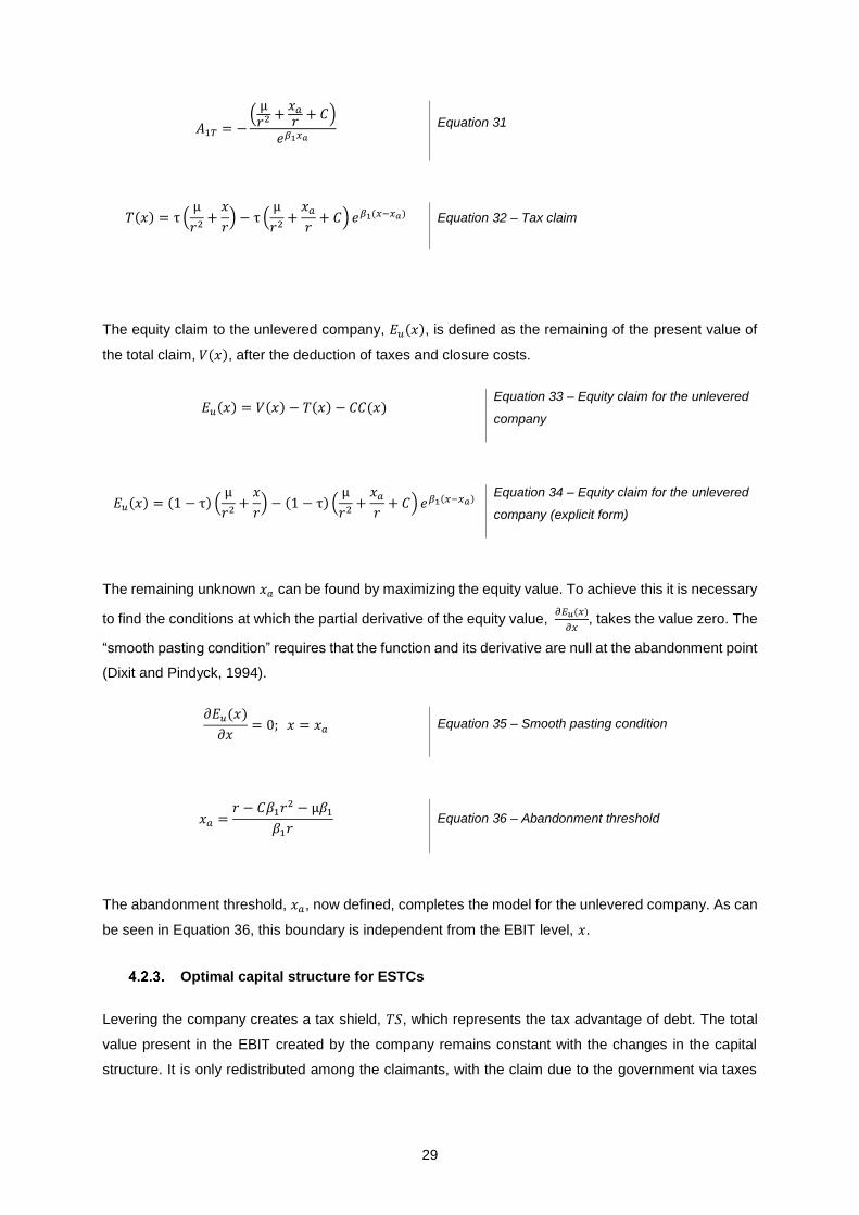
29

𝐴1𝑇 = −(

µ𝑟2 +

𝑥𝑎

𝑟+ 𝐶)

𝑒𝛽1𝑥𝑎

Equation 31

𝑇(𝑥) = τ (µ

𝑟2+

𝑥

𝑟) − τ (

µ

𝑟2+

𝑥𝑎

𝑟+ 𝐶) 𝑒𝛽1(𝑥−𝑥𝑎) Equation 32 – Tax claim

The equity claim to the unlevered company, 𝐸𝑢(𝑥), is defined as the remaining of the present value of

the total claim, 𝑉(𝑥), after the deduction of taxes and closure costs.

𝐸𝑢(𝑥) = 𝑉(𝑥) − 𝑇(𝑥) − 𝐶𝐶(𝑥) Equation 33 – Equity claim for the unlevered

company

𝐸𝑢(𝑥) = (1 − τ) (µ

𝑟2+

𝑥

𝑟) − (1 − τ) (

µ

𝑟2+

𝑥𝑎

𝑟+ 𝐶) 𝑒𝛽1(𝑥−𝑥𝑎)

Equation 34 – Equity claim for the unlevered

company (explicit form)

The remaining unknown 𝑥𝑎 can be found by maximizing the equity value. To achieve this it is necessary

to find the conditions at which the partial derivative of the equity value, 𝜕𝐸𝑢(𝑥)

𝜕𝑥, takes the value zero. The

“smooth pasting condition” requires that the function and its derivative are null at the abandonment point

(Dixit and Pindyck, 1994).

𝜕𝐸𝑢(𝑥)

𝜕𝑥= 0; 𝑥 = 𝑥𝑎 Equation 35 – Smooth pasting condition

𝑥𝑎 =𝑟 − 𝐶𝛽1𝑟2 − µ𝛽1

𝛽1𝑟 Equation 36 – Abandonment threshold

The abandonment threshold, 𝑥𝑎, now defined, completes the model for the unlevered company. As can

be seen in Equation 36, this boundary is independent from the EBIT level, 𝑥.

Optimal capital structure for ESTCs

Levering the company creates a tax shield, 𝑇𝑆, which represents the tax advantage of debt. The total

value present in the EBIT created by the company remains constant with the changes in the capital

structure. It is only redistributed among the claimants, with the claim due to the government via taxes

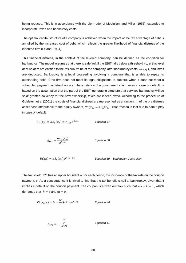
30

being reduced. This is in accordance with the pie model of Modigliani and Miller (1958), extended to

incorporate taxes and bankruptcy costs.

The optimal capital structure of a company is achieved when the impact of the tax advantage of debt is

annulled by the increased cost of debt, which reflects the greater likelihood of financial distress of the

indebted firm (Leland, 1994).

This financial distress, in the context of the levered company, can be defined as the condition for

bankruptcy. The model assumes that there is a default if the EBIT falls below a threshold 𝑥𝑏, at this level

debt holders are entitled to the residual value of the company, after bankruptcy costs, 𝐵𝐶(𝑥𝑏), and taxes

are deducted. Bankruptcy is a legal proceeding involving a company that is unable to repay its

outstanding debt. If the firm does not meet its legal obligations to debtors, when it does not meet a

scheduled payment, a default occurs. The existence of a government claim, even in case of default, is

based on the assumption that the part of the EBIT-generating structure that survives bankruptcy will be

sold: granted solvency for the new ownership, taxes are indeed owed. According to the procedure of

Goldstein et al (2001) the costs of financial distress are represented as a fraction, 𝛼, of the pre distress

asset base attributable to the equity owners, 𝐵𝐶(𝑥𝑏) = 𝛼𝐸𝑢(𝑥𝑏). That fraction is lost due to bankruptcy

in case of default.

𝐵𝐶(𝑥𝑏) = 𝛼𝐸𝑢(𝑥𝑏) = 𝐴1𝐵𝐶𝑒𝛽1𝑥𝑏 Equation 37

𝐴1𝐵𝐶 =𝛼𝐸𝑢(𝑥𝑏)

𝑒𝛽1𝑥𝑏 Equation 38

𝐵𝐶(𝑥) = 𝛼𝐸𝑢(𝑥𝑏)𝑒𝛽1(𝑥−𝑥𝑏) Equation 39 – Bankruptcy Costs claim

The tax shield, 𝑇𝑆, has an upper bound of 𝜏𝑐 for each period, the incidence of the tax rate on the coupon

payment, 𝑐. As a consequence it is trivial to find that the tax benefit is null at bankruptcy, given that it

implies a default on the coupon payment. The coupon is a fixed out flow such that 𝑚𝑥 + 𝑘 = 𝑐, which

demands that 𝑘 = 𝑐 and 𝑚 = 0.

𝑇𝑆(𝑥𝑏 , 𝑐) = 0 =𝜏𝑐

𝑟+ 𝐴1𝑇𝑆𝑒𝛽1𝑥𝑏 Equation 40

𝐴1𝑇𝑆 = −

𝜏𝑐𝑟

𝑒𝛽1𝑥𝑏 Equation 41

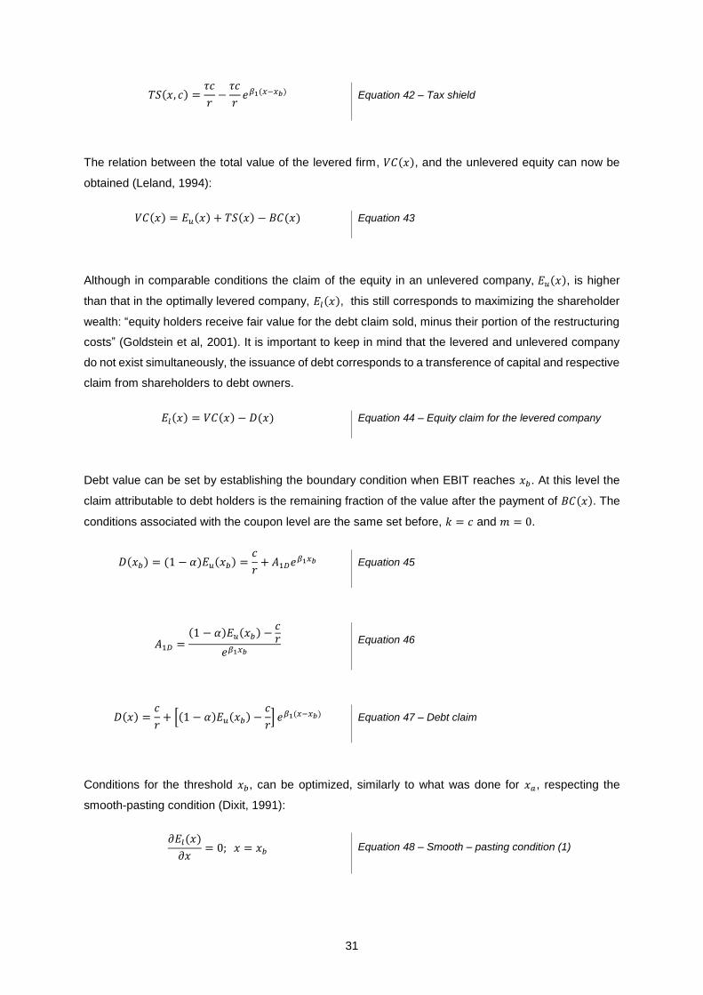
31

𝑇𝑆(𝑥, 𝑐) =𝜏𝑐

𝑟−

𝜏𝑐

𝑟𝑒𝛽1(𝑥−𝑥𝑏) Equation 42 – Tax shield

The relation between the total value of the levered firm, 𝑉𝐶(𝑥), and the unlevered equity can now be

obtained (Leland, 1994):

𝑉𝐶(𝑥) = 𝐸𝑢(𝑥) + 𝑇𝑆(𝑥) − 𝐵𝐶(𝑥) Equation 43

Although in comparable conditions the claim of the equity in an unlevered company, 𝐸𝑢(𝑥), is higher

than that in the optimally levered company, 𝐸𝑙(𝑥), this still corresponds to maximizing the shareholder

wealth: “equity holders receive fair value for the debt claim sold, minus their portion of the restructuring

costs” (Goldstein et al, 2001). It is important to keep in mind that the levered and unlevered company

do not exist simultaneously, the issuance of debt corresponds to a transference of capital and respective

claim from shareholders to debt owners.

𝐸𝑙(𝑥) = 𝑉𝐶(𝑥) − 𝐷(𝑥) Equation 44 – Equity claim for the levered company

Debt value can be set by establishing the boundary condition when EBIT reaches 𝑥𝑏. At this level the

claim attributable to debt holders is the remaining fraction of the value after the payment of 𝐵𝐶(𝑥). The

conditions associated with the coupon level are the same set before, 𝑘 = 𝑐 and 𝑚 = 0.

𝐷(𝑥𝑏) = (1 − 𝛼)𝐸𝑢(𝑥𝑏) =𝑐

𝑟+ 𝐴1𝐷𝑒𝛽1𝑥𝑏 Equation 45

𝐴1𝐷 =(1 − 𝛼)𝐸𝑢(𝑥𝑏) −

𝑐𝑟

𝑒𝛽1𝑥𝑏 Equation 46

𝐷(𝑥) =𝑐

𝑟+ [(1 − 𝛼)𝐸𝑢(𝑥𝑏) −

𝑐

𝑟] 𝑒𝛽1(𝑥−𝑥𝑏) Equation 47 – Debt claim

Conditions for the threshold 𝑥𝑏, can be optimized, similarly to what was done for 𝑥𝑎, respecting the

smooth-pasting condition (Dixit, 1991):

𝜕𝐸𝑙(𝑥)

𝜕𝑥= 0; 𝑥 = 𝑥𝑏 Equation 48 – Smooth – pasting condition (1)

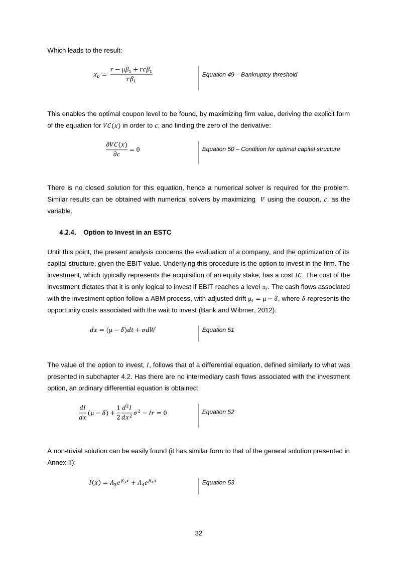
32

Which leads to the result:

𝑥𝑏 = 𝑟 − µ𝛽1 + 𝑟𝑐𝛽1

𝑟𝛽1

Equation 49 – Bankruptcy threshold

This enables the optimal coupon level to be found, by maximizing firm value, deriving the explicit form

of the equation for 𝑉𝐶(𝑥) in order to 𝑐, and finding the zero of the derivative:

𝜕𝑉𝐶(𝑥)

𝜕𝑐= 0 Equation 50 – Condition for optimal capital structure

There is no closed solution for this equation, hence a numerical solver is required for the problem.

Similar results can be obtained with numerical solvers by maximizing 𝑉 using the coupon, 𝑐, as the

variable.

Option to Invest in an ESTC

Until this point, the present analysis concerns the evaluation of a company, and the optimization of its

capital structure, given the EBIT value. Underlying this procedure is the option to invest in the firm. The

investment, which typically represents the acquisition of an equity stake, has a cost 𝐼𝐶. The cost of the

investment dictates that it is only logical to invest if EBIT reaches a level 𝑥𝑖. The cash flows associated

with the investment option follow a ABM process, with adjusted drift µ𝐼 = µ − 𝛿, where 𝛿 represents the

opportunity costs associated with the wait to invest (Bank and Wibmer, 2012).

𝑑𝑥 = (µ − 𝛿)𝑑𝑡 + 𝜎𝑑𝑊 Equation 51

The value of the option to invest, 𝐼, follows that of a differential equation, defined similarly to what was

presented in subchapter 4.2. Has there are no intermediary cash flows associated with the investment

option, an ordinary differential equation is obtained:

𝑑𝐼

𝑑𝑥(µ − 𝛿) +

1

2

𝑑2𝐼

𝑑𝑥2𝜎2 − 𝐼𝑟 = 0 Equation 52

A non-trivial solution can be easily found (it has similar form to that of the general solution presented in

Annex II):

𝐼(𝑥) = 𝐴3𝑒𝛽3𝑥 + 𝐴4𝑒𝛽4𝑥 Equation 53

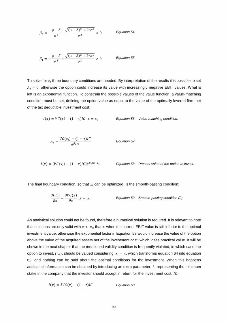
33

𝛽3 = −µ − 𝛿

𝜎2−

√(µ − 𝛿)2 + 2𝑟𝜎2

𝜎2< 0 Equation 54

𝛽4 = −µ − 𝛿

𝜎2+

√(µ − 𝛿)2 + 2𝑟𝜎2

𝜎2> 0 Equation 55

To solve for 𝑥𝑖 three boundary conditions are needed. By interpretation of the results it is possible to set

𝐴3 = 0, otherwise the option could increase its value with increasingly negative EBIT values. What is

left is an exponential function. To constrain the possible values of the value function, a value-matching

condition must be set, defining the option value as equal to the value of the optimally levered firm, net

of the tax deductible investment cost:

𝐼(𝑥) = 𝑉𝐶(𝑥) − (1 − 𝜏)𝐼𝐶, 𝑥 = 𝑥𝑖 Equation 56 – Value-matching condition.

𝐴4 =𝑉𝐶(𝑥𝑖) − (1 − 𝜏)𝐼𝐶

𝑒𝛽4𝑥𝑖 Equation 57

𝐼(𝑥) = [𝑉𝐶(𝑥𝑖) − (1 − 𝜏)𝐼𝐶]𝑒𝛽4(𝑥−𝑥𝑖) Equation 58 – Present value of the option to invest.

The final boundary condition, so that 𝑥𝑖 can be optimized, is the smooth-pasting condition:

𝜕𝐼(𝑥)

𝜕𝑥=

𝜕𝑉𝐶(𝑥)

𝜕𝑥; 𝑥 = 𝑥𝑖 Equation 59 – Smooth-pasting condition (2).

An analytical solution could not be found, therefore a numerical solution is required. It is relevant to note

that solutions are only valid with 𝑥 < 𝑥𝑖, that is when the current EBIT value is still inferior to the optimal

investment value, otherwise the exponential factor in Equation 58 would increase the value of the option

above the value of the acquired assets net of the investment cost, which loses practical value. It will be

shown in the next chapter that the mentioned validity condition is frequently violated, in which case the

option to invest, 𝐼(𝑥), should be valued considering 𝑥𝑖 = 𝑥, which transforms equation 64 into equation

62, and nothing can be said about the optimal conditions for the investment. When this happens

additional information can be obtained by introducing an extra parameter, 𝜆, representing the minimum

stake in the company that the investor should accept in return for the investment cost, 𝐼𝐶.

𝐼(𝑥) = 𝜆𝑉𝐶(𝑥) − (1 − 𝜏)𝐼𝐶 Equation 60

34

𝜆 =𝐼(𝑥) + (1 − 𝜏)𝐼𝐶

𝑉𝐶(𝑥) Equation 61 – Equity stake

The method applied in this subsection can be modified and replicated to reflect different options implied

in an investment process, as long as the assumption of dynamics described by an ABM would hold for

the real option. As an example, if used by the management of a company it could represent an option

to start a new project, in which case 𝑉𝐶(𝑥) would represent not the value of the company but of the

project, and 𝛿 would be measured in the present context of the company.

35

5. Case Study – Fitbit Inc.

The application of the model developed in the previous chapter to a real company provides insight into

the model that is not obtainable otherwise. The choice of Fitbit as the subject of study is a natural one,

it is a highly technological company, it went through a very recent and successful initial public offering

(IPO) and its success is derived of a unique combination between the fitness trackers that they sell and

the complementary software ecosystem, which constitutes a valuable set of IP. The ensuing valuation

of the company does not pretend to be a replica of the conditions that an investor faces when deciding

on a future investment, it is an academical exercise for which the most complete information available

was used. It can be argued that an investor in a pre-IPO moment would have access to undisclosed

information, which limits attempts to establish a scenario equivalent to a real case of investment. This

is particularly true for the parameters that are related with the simulation of the EBIT, for companies that

are not yet obtaining revenue, or that have had revenue for a limited amount of time, the estimates for

the simulation would have to be extracted indirectly from other data such as the user base, the market

size or more relevantly a valuation of the IP of the company.

Overview of the company

The term “wearables”, from wearable devices or technology, is transitioning from jargon used only by

technology enthusiasts, to a mainstream concept, mentioned daily in all forms of media. The term refers

to technological products that are incorporated into clothing or accessories to be worn directly on the

body. The number of categories into which wearable devices can be sorted is vast and constantly

increasing, including smartwatches, e-textiles, smart glasses, fitness trackers, among others. One of

the most successful companies to appear in the wearables market is Fitbit, headquartered in San

Francisco, USA. The main products of the company are a range of activity trackers: wireless enabled

devices, some used as wristbands others attachable to clothes, which incorporate multiple sensors in

order to record information such as the number of steps the user travels daily or the quality and quantity

of sleep. On May 2015, the company filed for IPO, to be listed in the New York Stock Exchange, eight

years after its funding in 2007. In the years anteceding the IPO, the company was financed by venture

capital firms, through four investment rounds, collecting a total of US$66M and reaching a valuation of

US$344M at the last round (Fitbit, 2015). The stock price soared from an opening value of US$20 to

US$31 in the first hours of trading, indicating a valuation of over US$6 billion (Yahoo, 2015).

Part of what distinguishes Fitbit is their platform, which can be accessed online or with a mobile app.

More than keeping record of the activity of each user, the platform performs has a social network keeping

users interested in the product, which can be a driver for future sales. The complete ecosystem that

sustains the competitive advantage of the company, from the user base to the mobile applications,

constitutes a valuable asset that could have been used to access debt capital and reduce the dilution of

ownership prior to the IPO, thus retaining more value for founders and early investors.

36

Despite its success, Fitbit faces relevant competition, from other brands of activity trackers, such as

Jawbone or Misfit; to potential substitute products such as Apple Watch and comparable offers from

other technological companies. A young company in an extremely competitive market, comprising

several of the biggest corporations in the world, carries a significant risk of not being able to sustain its

activity in the long run.

Financial data

One of the difficulties of the valuation of early stage companies, for academic purposes, is that, prior to

the IPO, little or no information is available to the general public. As part of the process to become a

publicly traded company, Fitbit was required to issue and divulge the S-1 Registration Statement, under

the Securities Act of 1993. This document is used as the source of all the financial information related

with Fitbit Inc. that is used in the ensuing analysis. The available data reaches back to 2010, including

a very comprehensive set of annual financial information.

Table 1 – Fitbit’s annual financial data (Fitbit, 2015)

2 2010 2011 2012 2013 2014

Values in million US dollars

Revenue 5.18 14.454 76.373 271.087 745.433

Operating income -1.366 -4.313 -3.775 -8.954 157.929

Net income -1.431 -4.317 -4.216 -51.622 131.777

The same document also provides quarterly data, for the period of June 2013 to March 2015. In order

to use the additional information provided by more data points, the measurements for the simulation of

EBIT will be based on quarterly values. To obtain the lacking values for the years 2010 to 2012, the

annual data for the year will be used, assuming that both the distribution of gross profit and operating

expenses follow the same variation pattern has those of the quarters of 20143.

Table 2 – Fitbit’s quarterly financial data (1) (Fitbit, 2015)

2 All the values in this work follow the same notation, using the dot as the decimal mark. 3 The year 2014 is chosen over 2013 due to the fact that at the end of the year the company had greatly increased

expenses due to a product recall.

1Q10 2Q10 3Q10 4Q10 1Q11 2Q11 3Q11 4Q11 1Q12 2Q12 3Q12

Values in million US dollars

Gross Profit 0.21 0.27 0.39 0.79 0.66 0.85 1.22 2.50 3.34 4.35 6.23

Operating Expenses

0.44 0.49 0.61 1.48 1.39 1.56 1.93 4.67 4.41 4.96 6.14

Operating Income

-0.23 -0.22 -0.22 -0.69 -0.73 -0.70 -0.70 -2.18 -1.08 -0.61 0.09

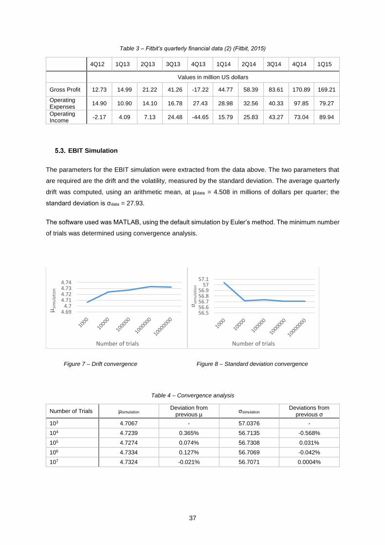
37

Table 3 – Fitbit’s quarterly financial data (2) (Fitbit, 2015)

4Q12 1Q13 2Q13 3Q13 4Q13 1Q14 2Q14 3Q14 4Q14 1Q15

Values in million US dollars

Gross Profit 12.73 14.99 21.22 41.26 -17.22 44.77 58.39 83.61 170.89 169.21

Operating Expenses

14.90 10.90 14.10 16.78 27.43 28.98 32.56 40.33 97.85 79.27

Operating Income

-2.17 4.09 7.13 24.48 -44.65 15.79 25.83 43.27 73.04 89.94

EBIT Simulation

The parameters for the EBIT simulation were extracted from the data above. The two parameters that

are required are the drift and the volatility, measured by the standard deviation. The average quarterly

drift was computed, using an arithmetic mean, at µdata = 4.508 in millions of dollars per quarter; the

standard deviation is σdata = 27.93.

The software used was MATLAB, using the default simulation by Euler’s method. The minimum number

of trials was determined using convergence analysis.

Figure 7 – Drift convergence Figure 8 – Standard deviation convergence

Table 4 – Convergence analysis

Number of Trials µsimulation Deviation from

previous µ σsimulation

Deviations from previous σ

103 4.7067 - 57.0376 -

104 4.7239 0.365% 56.7135 -0.568%

105 4.7274 0.074% 56.7308 0.031%

106 4.7334 0.127% 56.7069 -0.042%

107 4.7324 -0.021% 56.7071 0.0004%

4.694.7

4.714.724.734.74

µsi

mu

lati

on

Number of trials

56.556.656.756.856.9

5757.1

σsi

mu

lati

on

Number of trials

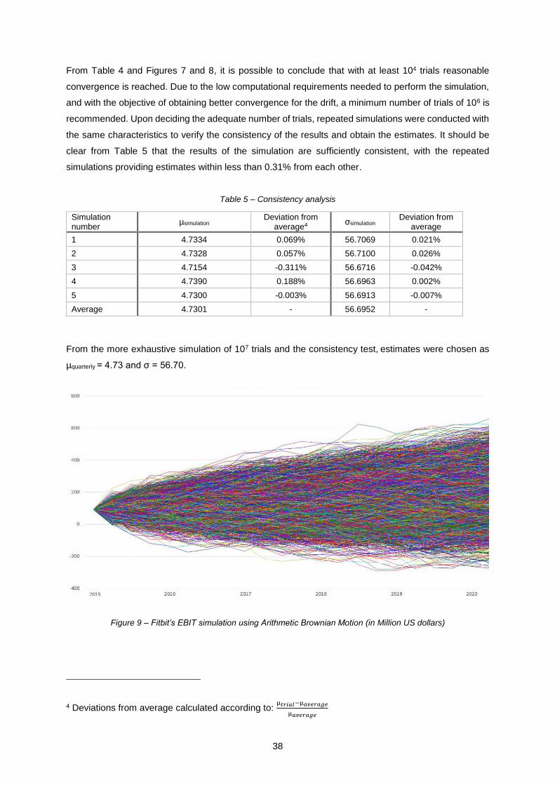
38

From Table 4 and Figures 7 and 8, it is possible to conclude that with at least 104 trials reasonable

convergence is reached. Due to the low computational requirements needed to perform the simulation,

and with the objective of obtaining better convergence for the drift, a minimum number of trials of 106 is

recommended. Upon deciding the adequate number of trials, repeated simulations were conducted with

the same characteristics to verify the consistency of the results and obtain the estimates. It should be

clear from Table 5 that the results of the simulation are sufficiently consistent, with the repeated

simulations providing estimates within less than 0.31% from each other.

Table 5 – Consistency analysis

Simulation number

µsimulation Deviation from

average4 σsimulation

Deviation from average

1 4.7334 0.069% 56.7069 0.021%

2 4.7328 0.057% 56.7100 0.026%

3 4.7154 -0.311% 56.6716 -0.042%

4 4.7390 0.188% 56.6963 0.002%

5 4.7300 -0.003% 56.6913 -0.007%

Average 4.7301 - 56.6952 -

From the more exhaustive simulation of 107 trials and the consistency test, estimates were chosen as

µquarterly = 4.73 and σ = 56.70.

Figure 9 – Fitbit’s EBIT simulation using Arithmetic Brownian Motion (in Million US dollars)

4 Deviations from average calculated according to: µ𝑡𝑟𝑖𝑎𝑙−µ𝑎𝑣𝑒𝑟𝑎𝑔𝑒

µ𝑎𝑣𝑒𝑟𝑎𝑔𝑒

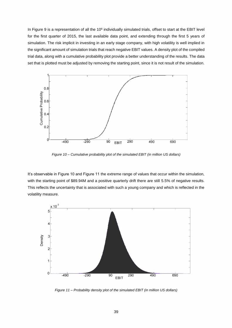
39

In Figure 9 is a representation of all the 106 individually simulated trials, offset to start at the EBIT level

for the first quarter of 2015, the last available data point, and extending through the first 5 years of

simulation. The risk implicit in investing in an early stage company, with high volatility is well implied in

the significant amount of simulation trials that reach negative EBIT values. A density plot of the compiled

trial data, along with a cumulative probability plot provide a better understanding of the results. The data

set that is plotted must be adjusted by removing the starting point, since it is not result of the simulation.

Figure 10 – Cumulative probability plot of the simulated EBIT (in million US dollars)

It’s observable in Figure 10 and Figure 11 the extreme range of values that occur within the simulation,

with the starting point of $89.94M and a positive quarterly drift there are still 5.5% of negative results.

This reflects the uncertainty that is associated with such a young company and which is reflected in the

volatility measure.

Figure 11 – Probability density plot of the simulated EBIT (in million US dollars)

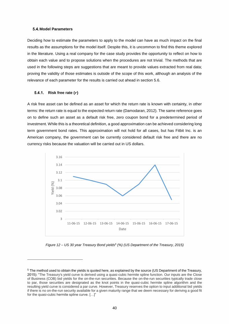
40

Model Parameters

Deciding how to estimate the parameters to apply to the model can have as much impact on the final

results as the assumptions for the model itself. Despite this, it is uncommon to find this theme explored

in the literature. Using a real company for the case study provides the opportunity to reflect on how to

obtain each value and to propose solutions when the procedures are not trivial. The methods that are

used in the following steps are suggestions that are meant to provide values extracted from real data;

proving the validity of those estimates is outside of the scope of this work, although an analysis of the

relevance of each parameter for the results is carried out ahead in section 5.6.

Risk free rate (𝒓)

A risk free asset can be defined as an asset for which the return rate is known with certainty, in other

terms: the return rate is equal to the expected return rate (Damodaran, 2012). The same reference goes

on to define such an asset as a default risk free, zero coupon bond for a predetermined period of

investment. While this is a theoretical definition, a good approximation can be achieved considering long

term government bond rates. This approximation will not hold for all cases, but has Fitbit Inc. is an

American company, the government can be currently considered default risk free and there are no

currency risks because the valuation will be carried out in US dollars.

Figure 12 – US 30 year Treasury Bond yields5 (%) (US Department of the Treasury, 2015)

5 The method used to obtain the yields is quoted here, as explained by the source (US Department of the Treasury,

2015): “The Treasury's yield curve is derived using a quasi-cubic hermite spline function. Our inputs are the Close of Business (COB) bid yields for the on-the-run securities. Because the on-the-run securities typically trade close to par, those securities are designated as the knot points in the quasi-cubic hermite spline algorithm and the resulting yield curve is considered a par curve. However, Treasury reserves the option to input additional bid yields if there is no on-the-run security available for a given maturity range that we deem necessary for deriving a good fit for the quasi-cubic hermite spline curve. […]”

3

3.02

3.04

3.06

3.08

3.1

3.12

3.14

3.16

11-06-15 12-06-15 13-06-15 14-06-15 15-06-15 16-06-15 17-06-15

Yiel

d (

%)

Date

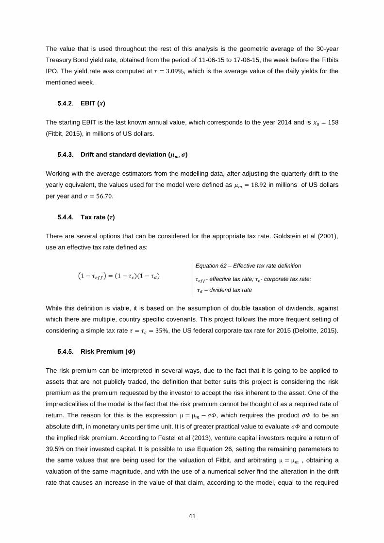
41

The value that is used throughout the rest of this analysis is the geometric average of the 30-year

Treasury Bond yield rate, obtained from the period of 11-06-15 to 17-06-15, the week before the Fitbits

IPO. The yield rate was computed at 𝑟 = 3.09%, which is the average value of the daily yields for the

mentioned week.

EBIT (𝒙)

The starting EBIT is the last known annual value, which corresponds to the year 2014 and is 𝑥0 = 158

(Fitbit, 2015), in millions of US dollars.

Drift and standard deviation (𝝁𝒎, 𝝈)

Working with the average estimators from the modelling data, after adjusting the quarterly drift to the

yearly equivalent, the values used for the model were defined as 𝜇𝑚 = 18.92 in millions of US dollars

per year and 𝜎 = 56.70.

Tax rate (𝝉)

There are several options that can be considered for the appropriate tax rate. Goldstein et al (2001),

use an effective tax rate defined as:

(1 − 𝜏𝑒𝑓𝑓) = (1 − 𝜏𝑐)(1 − 𝜏𝑑)

Equation 62 – Effective tax rate definition

𝜏𝑒𝑓𝑓- effective tax rate; 𝜏𝑐- corporate tax rate;

𝜏𝑑 – dividend tax rate

While this definition is viable, it is based on the assumption of double taxation of dividends, against

which there are multiple, country specific covenants. This project follows the more frequent setting of

considering a simple tax rate 𝜏 = 𝜏𝑐 = 35%, the US federal corporate tax rate for 2015 (Deloitte, 2015).

Risk Premium (𝜱)

The risk premium can be interpreted in several ways, due to the fact that it is going to be applied to

assets that are not publicly traded, the definition that better suits this project is considering the risk

premium as the premium requested by the investor to accept the risk inherent to the asset. One of the

impracticalities of the model is the fact that the risk premium cannot be thought of as a required rate of

return. The reason for this is the expression µ = µ𝑚 − 𝜎𝛷, which requires the product 𝜎𝛷 to be an

absolute drift, in monetary units per time unit. It is of greater practical value to evaluate 𝜎𝛷 and compute

the implied risk premium. According to Festel et al (2013), venture capital investors require a return of

39.5% on their invested capital. It is possible to use Equation 26, setting the remaining parameters to

the same values that are being used for the valuation of Fitbit, and arbitrating µ = µ𝑚 , obtaining a

valuation of the same magnitude, and with the use of a numerical solver find the alteration in the drift

rate that causes an increase in the value of that claim, according to the model, equal to the required

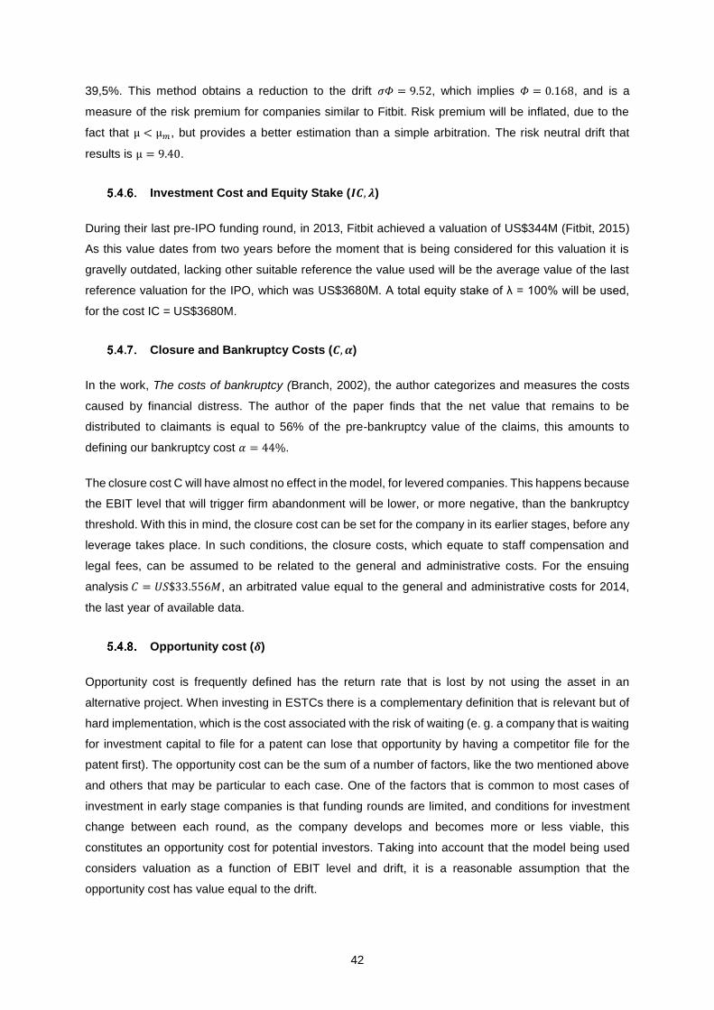
42

39,5%. This method obtains a reduction to the drift 𝜎𝛷 = 9.52, which implies 𝛷 = 0.168, and is a

measure of the risk premium for companies similar to Fitbit. Risk premium will be inflated, due to the

fact that µ < µ𝑚, but provides a better estimation than a simple arbitration. The risk neutral drift that

results is µ = 9.40.

Investment Cost and Equity Stake (𝑰𝑪, 𝝀)

During their last pre-IPO funding round, in 2013, Fitbit achieved a valuation of US$344M (Fitbit, 2015)

As this value dates from two years before the moment that is being considered for this valuation it is

gravelly outdated, lacking other suitable reference the value used will be the average value of the last

reference valuation for the IPO, which was US$3680M. A total equity stake of λ = 100% will be used,

for the cost IC = US$3680M.

Closure and Bankruptcy Costs (𝑪, 𝜶)

In the work, The costs of bankruptcy (Branch, 2002), the author categorizes and measures the costs

caused by financial distress. The author of the paper finds that the net value that remains to be

distributed to claimants is equal to 56% of the pre-bankruptcy value of the claims, this amounts to

defining our bankruptcy cost 𝛼 = 44%.

The closure cost C will have almost no effect in the model, for levered companies. This happens because

the EBIT level that will trigger firm abandonment will be lower, or more negative, than the bankruptcy

threshold. With this in mind, the closure cost can be set for the company in its earlier stages, before any

leverage takes place. In such conditions, the closure costs, which equate to staff compensation and

legal fees, can be assumed to be related to the general and administrative costs. For the ensuing

analysis 𝐶 = 𝑈𝑆$33.556𝑀, an arbitrated value equal to the general and administrative costs for 2014,

the last year of available data.

Opportunity cost (𝜹)

Opportunity cost is frequently defined has the return rate that is lost by not using the asset in an

alternative project. When investing in ESTCs there is a complementary definition that is relevant but of

hard implementation, which is the cost associated with the risk of waiting (e. g. a company that is waiting

for investment capital to file for a patent can lose that opportunity by having a competitor file for the

patent first). The opportunity cost can be the sum of a number of factors, like the two mentioned above

and others that may be particular to each case. One of the factors that is common to most cases of

investment in early stage companies is that funding rounds are limited, and conditions for investment

change between each round, as the company develops and becomes more or less viable, this

constitutes an opportunity cost for potential investors. Taking into account that the model being used

considers valuation as a function of EBIT level and drift, it is a reasonable assumption that the

opportunity cost has value equal to the drift.

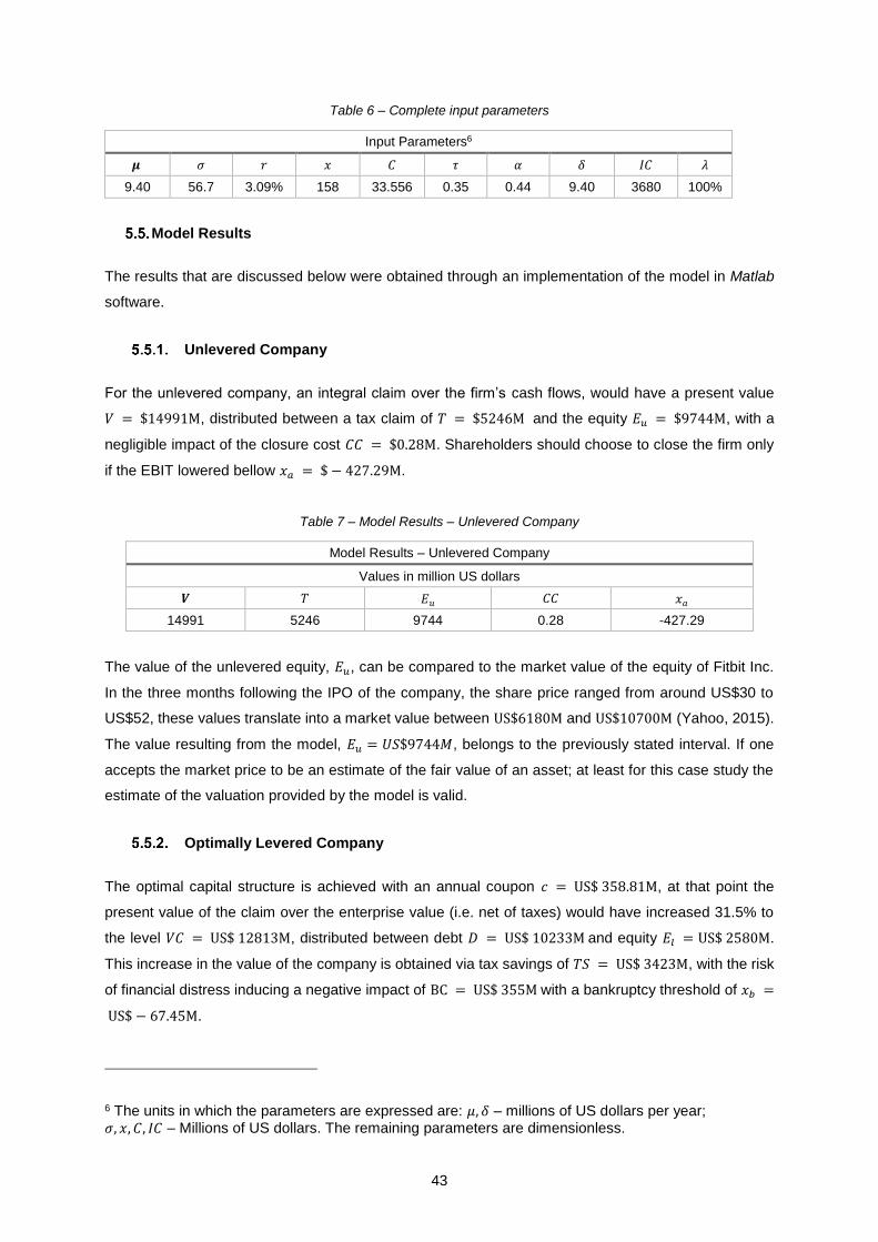
43

Table 6 – Complete input parameters

Input Parameters6

𝝁 𝜎 𝑟 𝑥 𝐶 𝜏 𝛼 𝛿 𝐼𝐶 𝜆

9.40 56.7 3.09% 158 33.556 0.35 0.44 9.40 3680 100%

Model Results

The results that are discussed below were obtained through an implementation of the model in Matlab

software.

Unlevered Company

For the unlevered company, an integral claim over the firm’s cash flows, would have a present value

𝑉 = $14991M, distributed between a tax claim of 𝑇 = $5246M and the equity 𝐸𝑢 = $9744M, with a

negligible impact of the closure cost 𝐶𝐶 = $0.28M. Shareholders should choose to close the firm only

if the EBIT lowered bellow 𝑥𝑎 = $ − 427.29M.

Table 7 – Model Results – Unlevered Company

Model Results – Unlevered Company

Values in million US dollars

𝑽 𝑇 𝐸𝑢 𝐶𝐶 𝑥𝑎

14991 5246 9744 0.28 -427.29

The value of the unlevered equity, 𝐸𝑢, can be compared to the market value of the equity of Fitbit Inc.

In the three months following the IPO of the company, the share price ranged from around US$30 to

US$52, these values translate into a market value between US$6180M and US$10700M (Yahoo, 2015).

The value resulting from the model, 𝐸𝑢 = 𝑈𝑆$9744𝑀, belongs to the previously stated interval. If one

accepts the market price to be an estimate of the fair value of an asset; at least for this case study the

estimate of the valuation provided by the model is valid.

Optimally Levered Company

The optimal capital structure is achieved with an annual coupon 𝑐 = US$ 358.81M, at that point the

present value of the claim over the enterprise value (i.e. net of taxes) would have increased 31.5% to

the level 𝑉𝐶 = US$ 12813M, distributed between debt 𝐷 = US$ 10233M and equity 𝐸𝑙 = US$ 2580M.

This increase in the value of the company is obtained via tax savings of 𝑇𝑆 = US$ 3423M, with the risk

of financial distress inducing a negative impact of BC = US$ 355M with a bankruptcy threshold of 𝑥𝑏 =

US$ − 67.45M.

6 The units in which the parameters are expressed are: 𝜇, 𝛿 – millions of US dollars per year; 𝜎, 𝑥, 𝐶, 𝐼𝐶 – Millions of US dollars. The remaining parameters are dimensionless.

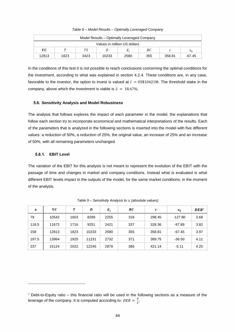
44

Table 8 – Model Results – Optimally Leveraged Company

Model Results – Optimally Leveraged Company

Values in million US dollars

𝑽𝑪 𝑇 𝑇𝑆 𝐷 𝐸𝑙 𝐵𝐶 𝑐 𝑥𝑏

12813 1823 3423 10233 2580 355 358.81 -67.45

In the conditions of this test it is not possible to reach conclusions concerning the optimal conditions for

the investment, according to what was explained in section 4.2.4. These conditions are, in any case,

favorable to the investor, the option to invest is valued at 𝐼 = US$10421M. The threshold stake in the

company, above which the investment is viable is 𝜆 = 18.67%.

Sensitivity Analysis and Model Robustness

The analysis that follows explores the impact of each parameter in the model, the explanations that

follow each section try to incorporate economical and mathematical interpretations of the results. Each

of the parameters that is analyzed in the following sections is inserted into the model with five different

values: a reduction of 50%, a reduction of 25%, the original value, an increase of 25% and an increase

of 50%, with all remaining parameters unchanged.

EBIT Level

The variation of the EBIT for this analysis is not meant to represent the evolution of the EBIT with the

passage of time and changes in market and company conditions. Instead what is evaluated is what

different EBIT levels impact in the outputs of the model, for the same market conditions, in the moment

of the analysis.

Table 9 – Sensitivity Analysis to 𝑥 (absolute values)

𝒙 𝑽𝑪 𝑻 𝑫 𝑬𝒍 𝑩𝑪 𝒄 𝒙𝒃 𝑫𝑬𝑹7

79 10542 1603 8289 2255 318 298.45 -127.80 3.68

118.5 11672 1716 9251 2421 337 328.36 -97.89 3.82

158 12813 1823 10233 2580 355 358.81 -67.45 3.97

197.5 13964 1925 11231 2732 371 389.75 -36.50 4.11

237 15124 2022 12245 2879 386 421.14 -5.11 4.25

7 Debt-to-Equity ratio – this financial ratio will be used in the following sections as a measure of the

leverage of the company. It is computed according to: 𝐷𝐸𝑅 = 𝐷

𝐸.

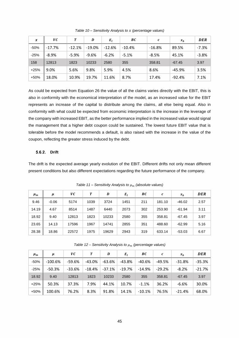
45

Table 10 – Sensitivity Analysis to 𝑥 (percentage values)

𝒙 𝑽𝑪 𝑻 𝑫 𝑬𝒍 𝑩𝑪 𝒄 𝒙𝒃 𝑫𝑬𝑹

-50% -17.7% -12.1% -19.0% -12.6% -10.4% -16.8% 89.5% -7.3%

-25% -8.9% -5.9% -9.6% -6.2% -5.1% -8.5% 45.1% -3.8%

158 12813 1823 10233 2580 355 358.81 -67.45 3.97

+25% 9.0% 5.6% 9.8% 5.9% 4.5% 8.6% -45.9% 3.5%

+50% 18.0% 10.9% 19.7% 11.6% 8.7% 17.4% -92.4% 7.1%

As could be expected from Equation 26 the value of all the claims varies directly with the EBIT, this is

also in conformity with the economical interpretation of the model, as an increased value for the EBIT

represents an increase of the capital to distribute among the claims, all else being equal. Also in

conformity with what could be expected from economic interpretation is the increase in the leverage of

the company with increased EBIT, as the better performance implied in the increased value would signal

the management that a higher debt coupon could be sustained. The lowest future EBIT value that is

tolerable before the model recommends a default, is also raised with the increase in the value of the

coupon, reflecting the greater stress induced by the debt.

Drift

The drift is the expected average yearly evolution of the EBIT. Different drifts not only mean different

present conditions but also different expectations regarding the future performance of the company.

Table 11 – Sensitivity Analysis to 𝜇𝑚 (absolute values)

𝝁𝒎 𝝁 𝑽𝑪 𝑻 𝑫 𝑬𝒍 𝑩𝑪 𝒄 𝒙𝒃 𝑫𝑬𝑹

9.46 -0.06 5174 1039 3724 1451 211 181.10 -46.02 2.57

14.19 4.67 8514 1487 6440 2073 302 253.90 -61.94 3.11

18.92 9.40 12813 1823 10233 2580 355 358.81 -67.45 3.97

23.65 14.13 17596 1967 14741 2855 351 488.60 -62.99 5.16

28.38 18.86 22572 1975 19629 2943 319 633.14 -53.03 6.67

Table 12 – Sensitivity Analysis to 𝜇𝑚 (percentage values)

𝝁𝒎 𝝁 𝑽𝑪 𝑻 𝑫 𝑬𝒍 𝑩𝑪 𝒄 𝒙𝒃 𝑫𝑬𝑹

-50% -100.6% -59.6% -43.0% -63.6% -43.8% -40.6% -49.5% -31.8% -35.3%

-25% -50.3% -33.6% -18.4% -37.1% -19.7% -14.9% -29.2% -8.2% -21.7%

18.92 9.40 12813 1823 10233 2580 355 358.81 -67.45 3.97

+25% 50.3% 37.3% 7.9% 44.1% 10.7% -1.1% 36.2% -6.6% 30.0%

+50% 100.6% 76.2% 8.3% 91.8% 14.1% -10.1% 76.5% -21.4% 68.0%

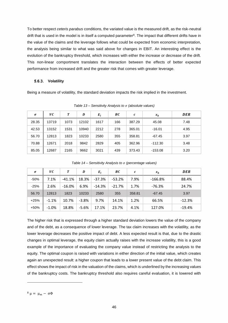
46

To better respect ceteris parabus conditions, the variated value is the measured drift, as the risk-neutral

drift that is used in the model is in itself a computed parameter8. The impact that different drifts have in

the value of the claims and the leverage follows what could be expected from economic interpretation,

the analysis being similar to what was said above for changes in EBIT. An interesting effect is the

evolution of the bankruptcy threshold, which increases with either the increase or decrease of the drift.

This non-linear comportment translates the interaction between the effects of better expected

performance from increased drift and the greater risk that comes with greater leverage.

Volatility

Being a measure of volatility, the standard deviation impacts the risk implied in the investment.

Table 13 – Sensitivity Analysis to 𝜎 (absolute values)

𝝈 𝑽𝑪 𝑻 𝑫 𝑬𝒍 𝑩𝑪 𝒄 𝒙𝒃 𝑫𝑬𝑹

28.35 13719 1073 12102 1617 166 387.29 45.08 7.48

42.53 13152 1531 10940 2212 278 365.01 -16.01 4.95

56.70 12813 1823 10233 2580 355 358.81 -67.45 3.97

70.88 12671 2018 9842 2829 405 362.96 -112.30 3.48

85.05 12687 2165 9662 3021 439 373.43 -153.08 3.20

Table 14 – Sensitivity Analysis to 𝜎 (percentage values)

𝝈 𝑽𝑪 𝑻 𝑫 𝑬𝒍 𝑩𝑪 𝒄 𝒙𝒃 𝑫𝑬𝑹

-50% 7.1% -41.1% 18.3% -37.3% -53.2% 7.9% -166.8% 88.4%

-25% 2.6% -16.0% 6.9% -14.3% -21.7% 1.7% -76.3% 24.7%

56.70 12813 1823 10233 2580 355 358.81 -67.45 3.97

+25% -1.1% 10.7% -3.8% 9.7% 14.1% 1.2% 66.5% -12.3%

+50% -1.0% 18.8% -5.6% 17.1% 23.7% 4.1% 127.0% -19.4%

The higher risk that is expressed through a higher standard deviation lowers the value of the company

and of the debt, as a consequence of lower leverage. The tax claim increases with the volatility, as the

lower leverage decreases the positive impact of debt. A less expected result is that, due to the drastic

changes in optimal leverage, the equity claim actually raises with the increase volatility, this is a good

example of the importance of evaluating the company value instead of restricting the analysis to the

equity. The optimal coupon is raised with variations in either direction of the initial value, which creates

again an unexpected result: a higher coupon that leads to a lower present value of the debt claim. This

effect shows the impact of risk in the valuation of the claims, which is underlined by the increasing values

of the bankruptcy costs. The bankruptcy threshold also requires careful evaluation, it is lowered with

8 µ = µ𝑚 − σΦ

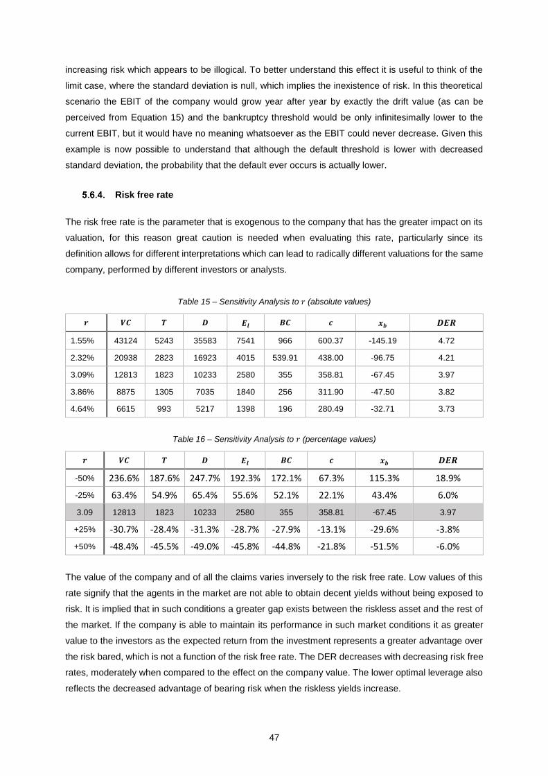
47

increasing risk which appears to be illogical. To better understand this effect it is useful to think of the

limit case, where the standard deviation is null, which implies the inexistence of risk. In this theoretical

scenario the EBIT of the company would grow year after year by exactly the drift value (as can be

perceived from Equation 15) and the bankruptcy threshold would be only infinitesimally lower to the

current EBIT, but it would have no meaning whatsoever as the EBIT could never decrease. Given this

example is now possible to understand that although the default threshold is lower with decreased

standard deviation, the probability that the default ever occurs is actually lower.

Risk free rate

The risk free rate is the parameter that is exogenous to the company that has the greater impact on its

valuation, for this reason great caution is needed when evaluating this rate, particularly since its

definition allows for different interpretations which can lead to radically different valuations for the same

company, performed by different investors or analysts.

Table 15 – Sensitivity Analysis to 𝑟 (absolute values)

𝒓 𝑽𝑪 𝑻 𝑫 𝑬𝒍 𝑩𝑪 𝒄 𝒙𝒃 𝑫𝑬𝑹

1.55% 43124 5243 35583 7541 966 600.37 -145.19 4.72

2.32% 20938 2823 16923 4015 539.91 438.00 -96.75 4.21

3.09% 12813 1823 10233 2580 355 358.81 -67.45 3.97

3.86% 8875 1305 7035 1840 256 311.90 -47.50 3.82

4.64% 6615 993 5217 1398 196 280.49 -32.71 3.73

Table 16 – Sensitivity Analysis to 𝑟 (percentage values)

𝒓 𝑽𝑪 𝑻 𝑫 𝑬𝒍 𝑩𝑪 𝒄 𝒙𝒃 𝑫𝑬𝑹

-50% 236.6% 187.6% 247.7% 192.3% 172.1% 67.3% 115.3% 18.9%

-25% 63.4% 54.9% 65.4% 55.6% 52.1% 22.1% 43.4% 6.0%

3.09 12813 1823 10233 2580 355 358.81 -67.45 3.97

+25% -30.7% -28.4% -31.3% -28.7% -27.9% -13.1% -29.6% -3.8%

+50% -48.4% -45.5% -49.0% -45.8% -44.8% -21.8% -51.5% -6.0%

The value of the company and of all the claims varies inversely to the risk free rate. Low values of this

rate signify that the agents in the market are not able to obtain decent yields without being exposed to

risk. It is implied that in such conditions a greater gap exists between the riskless asset and the rest of

the market. If the company is able to maintain its performance in such market conditions it as greater

value to the investors as the expected return from the investment represents a greater advantage over

the risk bared, which is not a function of the risk free rate. The DER decreases with decreasing risk free

rates, moderately when compared to the effect on the company value. The lower optimal leverage also

reflects the decreased advantage of bearing risk when the riskless yields increase.

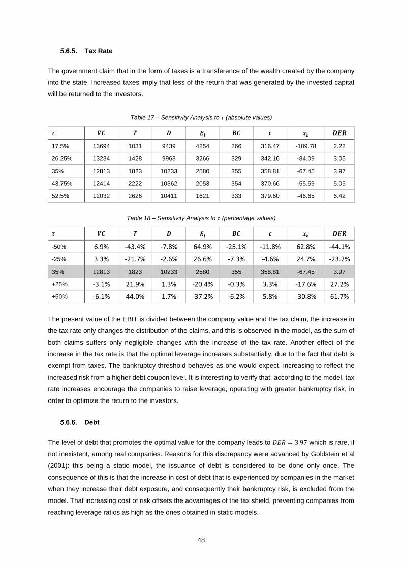
48

Tax Rate

The government claim that in the form of taxes is a transference of the wealth created by the company

into the state. Increased taxes imply that less of the return that was generated by the invested capital

will be returned to the investors.

Table 17 – Sensitivity Analysis to 𝜏 (absolute values)

𝝉 𝑽𝑪 𝑻 𝑫 𝑬𝒍 𝑩𝑪 𝒄 𝒙𝒃 𝑫𝑬𝑹

17.5% 13694 1031 9439 4254 266 316.47 -109.78 2.22

26.25% 13234 1428 9968 3266 329 342.16 -84.09 3.05

35% 12813 1823 10233 2580 355 358.81 -67.45 3.97

43.75% 12414 2222 10362 2053 354 370.66 -55.59 5.05

52.5% 12032 2626 10411 1621 333 379.60 -46.65 6.42

Table 18 – Sensitivity Analysis to 𝜏 (percentage values)

𝝉 𝑽𝑪 𝑻 𝑫 𝑬𝒍 𝑩𝑪 𝒄 𝒙𝒃 𝑫𝑬𝑹

-50% 6.9% -43.4% -7.8% 64.9% -25.1% -11.8% 62.8% -44.1%

-25% 3.3% -21.7% -2.6% 26.6% -7.3% -4.6% 24.7% -23.2%

35% 12813 1823 10233 2580 355 358.81 -67.45 3.97

+25% -3.1% 21.9% 1.3% -20.4% -0.3% 3.3% -17.6% 27.2%

+50% -6.1% 44.0% 1.7% -37.2% -6.2% 5.8% -30.8% 61.7%

The present value of the EBIT is divided between the company value and the tax claim, the increase in

the tax rate only changes the distribution of the claims, and this is observed in the model, as the sum of

both claims suffers only negligible changes with the increase of the tax rate. Another effect of the

increase in the tax rate is that the optimal leverage increases substantially, due to the fact that debt is

exempt from taxes. The bankruptcy threshold behaves as one would expect, increasing to reflect the

increased risk from a higher debt coupon level. It is interesting to verify that, according to the model, tax

rate increases encourage the companies to raise leverage, operating with greater bankruptcy risk, in

order to optimize the return to the investors.

Debt

The level of debt that promotes the optimal value for the company leads to 𝐷𝐸𝑅 = 3.97 which is rare, if

not inexistent, among real companies. Reasons for this discrepancy were advanced by Goldstein et al

(2001): this being a static model, the issuance of debt is considered to be done only once. The

consequence of this is that the increase in cost of debt that is experienced by companies in the market

when they increase their debt exposure, and consequently their bankruptcy risk, is excluded from the

model. That increasing cost of risk offsets the advantages of the tax shield, preventing companies from

reaching leverage ratios as high as the ones obtained in static models.

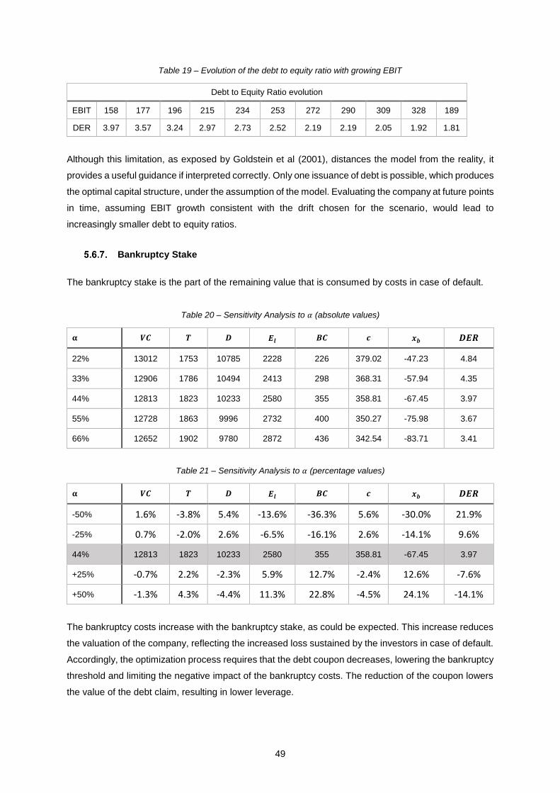
49

Table 19 – Evolution of the debt to equity ratio with growing EBIT

Debt to Equity Ratio evolution

EBIT 158 177 196 215 234 253 272 290 309 328 189

DER 3.97 3.57 3.24 2.97 2.73 2.52 2.19 2.19 2.05 1.92 1.81

Although this limitation, as exposed by Goldstein et al (2001), distances the model from the reality, it

provides a useful guidance if interpreted correctly. Only one issuance of debt is possible, which produces

the optimal capital structure, under the assumption of the model. Evaluating the company at future points

in time, assuming EBIT growth consistent with the drift chosen for the scenario, would lead to

increasingly smaller debt to equity ratios.

Bankruptcy Stake

The bankruptcy stake is the part of the remaining value that is consumed by costs in case of default.

Table 20 – Sensitivity Analysis to 𝛼 (absolute values)

𝛂 𝑽𝑪 𝑻 𝑫 𝑬𝒍 𝑩𝑪 𝒄 𝒙𝒃 𝑫𝑬𝑹

22% 13012 1753 10785 2228 226 379.02 -47.23 4.84

33% 12906 1786 10494 2413 298 368.31 -57.94 4.35

44% 12813 1823 10233 2580 355 358.81 -67.45 3.97

55% 12728 1863 9996 2732 400 350.27 -75.98 3.67

66% 12652 1902 9780 2872 436 342.54 -83.71 3.41

Table 21 – Sensitivity Analysis to 𝛼 (percentage values)

𝛂 𝑽𝑪 𝑻 𝑫 𝑬𝒍 𝑩𝑪 𝒄 𝒙𝒃 𝑫𝑬𝑹

-50% 1.6% -3.8% 5.4% -13.6% -36.3% 5.6% -30.0% 21.9%

-25% 0.7% -2.0% 2.6% -6.5% -16.1% 2.6% -14.1% 9.6%

44% 12813 1823 10233 2580 355 358.81 -67.45 3.97

+25% -0.7% 2.2% -2.3% 5.9% 12.7% -2.4% 12.6% -7.6%

+50% -1.3% 4.3% -4.4% 11.3% 22.8% -4.5% 24.1% -14.1%

The bankruptcy costs increase with the bankruptcy stake, as could be expected. This increase reduces

the valuation of the company, reflecting the increased loss sustained by the investors in case of default.

Accordingly, the optimization process requires that the debt coupon decreases, lowering the bankruptcy

threshold and limiting the negative impact of the bankruptcy costs. The reduction of the coupon lowers

the value of the debt claim, resulting in lower leverage.

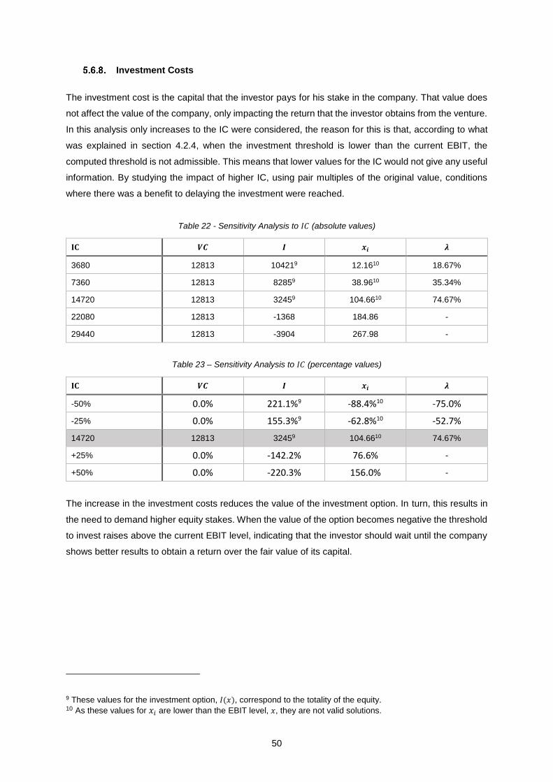
50

Investment Costs

The investment cost is the capital that the investor pays for his stake in the company. That value does

not affect the value of the company, only impacting the return that the investor obtains from the venture.

In this analysis only increases to the IC were considered, the reason for this is that, according to what

was explained in section 4.2.4, when the investment threshold is lower than the current EBIT, the

computed threshold is not admissible. This means that lower values for the IC would not give any useful

information. By studying the impact of higher IC, using pair multiples of the original value, conditions

where there was a benefit to delaying the investment were reached.

Table 22 - Sensitivity Analysis to 𝐼𝐶 (absolute values)

𝐈𝐂 𝑽𝑪 𝑰 𝒙𝒊 𝝀

3680 12813 104219 12.1610 18.67%

7360 12813 82859 38.9610 35.34%

14720 12813 32459 104.6610 74.67%

22080 12813 -1368 184.86 -

29440 12813 -3904 267.98 -

Table 23 – Sensitivity Analysis to 𝐼𝐶 (percentage values)

𝐈𝐂 𝑽𝑪 𝑰 𝒙𝒊 𝝀

-50% 0.0% 221.1%9 -88.4%10 -75.0%

-25% 0.0% 155.3%9 -62.8%10 -52.7%

14720 12813 32459 104.6610 74.67%

+25% 0.0% -142.2% 76.6% -

+50% 0.0% -220.3% 156.0% -

The increase in the investment costs reduces the value of the investment option. In turn, this results in

the need to demand higher equity stakes. When the value of the option becomes negative the threshold

to invest raises above the current EBIT level, indicating that the investor should wait until the company

shows better results to obtain a return over the fair value of its capital.

9 These values for the investment option, 𝐼(𝑥), correspond to the totality of the equity. 10 As these values for 𝑥𝑖 are lower than the EBIT level, 𝑥, they are not valid solutions.

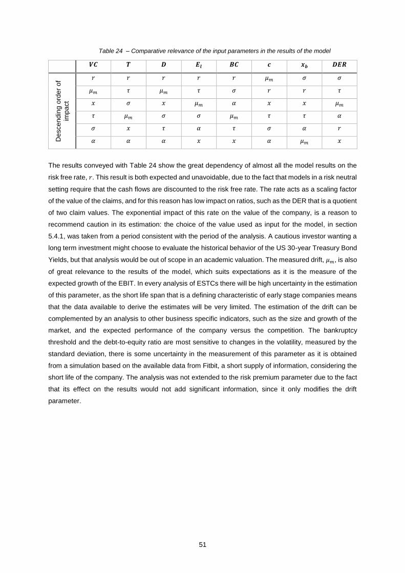
51

Table 24 – Comparative relevance of the input parameters in the results of the model

𝑽𝑪 𝑻 𝑫 𝑬𝒍 𝑩𝑪 𝒄 𝒙𝒃 𝑫𝑬𝑹 D

escendin

g o

rder

of

imp

act

𝑟 𝑟 𝑟 𝑟 𝑟 𝜇𝑚 𝜎 𝜎

𝜇𝑚 𝜏 𝜇𝑚 𝜏 𝜎 𝑟 𝑟 𝜏

𝑥 𝜎 𝑥 𝜇𝑚 𝛼 𝑥 𝑥 𝜇𝑚

𝜏 𝜇𝑚 𝜎 𝜎 𝜇𝑚 𝜏 𝜏 𝛼

𝜎 𝑥 𝜏 𝛼 𝜏 𝜎 𝛼 𝑟

𝛼 𝛼 𝛼 𝑥 𝑥 𝛼 𝜇𝑚 𝑥

The results conveyed with Table 24 show the great dependency of almost all the model results on the

risk free rate, 𝑟. This result is both expected and unavoidable, due to the fact that models in a risk neutral

setting require that the cash flows are discounted to the risk free rate. The rate acts as a scaling factor

of the value of the claims, and for this reason has low impact on ratios, such as the DER that is a quotient

of two claim values. The exponential impact of this rate on the value of the company, is a reason to

recommend caution in its estimation: the choice of the value used as input for the model, in section

5.4.1, was taken from a period consistent with the period of the analysis. A cautious investor wanting a

long term investment might choose to evaluate the historical behavior of the US 30-year Treasury Bond

Yields, but that analysis would be out of scope in an academic valuation. The measured drift, 𝜇𝑚, is also

of great relevance to the results of the model, which suits expectations as it is the measure of the

expected growth of the EBIT. In every analysis of ESTCs there will be high uncertainty in the estimation

of this parameter, as the short life span that is a defining characteristic of early stage companies means

that the data available to derive the estimates will be very limited. The estimation of the drift can be

complemented by an analysis to other business specific indicators, such as the size and growth of the

market, and the expected performance of the company versus the competition. The bankruptcy

threshold and the debt-to-equity ratio are most sensitive to changes in the volatility, measured by the

standard deviation, there is some uncertainty in the measurement of this parameter as it is obtained

from a simulation based on the available data from Fitbit, a short supply of information, considering the

short life of the company. The analysis was not extended to the risk premium parameter due to the fact

that its effect on the results would not add significant information, since it only modifies the drift

parameter.

52

6. Conclusions

This work had for its foremost objective to contribute to the literature related with the study of the

valuation of ESTCs. By employing a structural model with the assumption that the EBIT of the company

can be modelled with an ABM, it was possible to do a valuation of the company and study its optimal

capital structure. The application of the model to a case study based on Fitbit Inc lead to a valuation

consistent with the market value of the company.

The methodology suited the objectives and object of study. The valuation of these companies requires

specific models, suited to deal with their particularities. Real options analysis meets the requirements,

particularly the incorporation of the volatility on the valuation to represent the uncertainty associated

with the underlying assets, in this case the EBIT of the early stage companies. These models also allow

increased flexibility, enabling the incorporation of events such as options to pursue new projects, delay

investments or expand existing ones, among many others. Having originated from the pricing of financial

options, many of these models share underlying assumptions that make them unsuitable to the

conditions faced by ESTCs.

The field of study of structural models, which incorporates the optimization of the capital structure in the

valuation process, offers increased possibilities to both management and investors, going beyond the

limiting assumption of all equity financing to consider the use of debt in the fulfillment of the capital

necessities of the company. This new option is useful for the management, enabling new sources of

financing capital, and creates value to investors, maximizing the value of the company through tax

savings and avoiding dilution of the equity. Selecting the EBIT as the state variable, creates an

economically meaningful representation of the operations, separating the generation of cash flows that

is due to the core activities of the company from the claims over those flows.

Early stage companies are highly susceptible to periods of negative earnings, and to not being long

lasted. Assuming otherwise is a compromise that skews the reality of the sector and limits the usefulness

of the analysis. Basing the dynamics of the state variable on an ABM, although so far uncommon in the

literature, is a valid solution to allow negative values for the EBIT. The proposed model, built on these

assumptions, is a flexible base that can be easily implemented and expanded.

A careful sensitivity and robustness study lead to a better understanding of the model, revealing its

limiting factors and the relevancy of each parameter on the results obtained. A critical assessment of

the results of this study created the opportunity to suggest solutions to the limitations found. The results

of the valuation are highly sensitive to changes in the risk free rate; there is uncertainty in the long term

estimates of this parameter that must be considered. The volatility parameter also has considerable

impact in the results, particularly in the optimal leverage proposed by the model. Providing estimates for

this parameter is one of the biggest challenges in the application of real options models to ESTCs, due

to the lack of available data on which to base the simulations. Working within a static framework for the

leverage of the company, leads to unreasonably high leverage ratios. As the value of the coupon

remains constant, an assessment of the debt to equity ratio with the expected evolution of the EBIT,

53

shows that the leverage will diminish with time, converging to more reasonable results. An interpretation

of the results of this model, that brings it closer to reality, is to treat the optimal coupon as a limit,

increasing the debt to reach it as the company evolves, rather than as a starting and fix value.

The application of the model to a reality based setting is a relevant contribution to the available literature,

since it is, to the extension of the author knowledge, the first case study for a structural model based on

a real ESTC. The results indicate that there is a relation between the value of the company and its

capital structure, resulting from the fiscal advantage to debt.

54

7. Bibliography

AJPark, n.d. Guide to Royalties and Licence Fees. Available at: < http://www.ajpark.com/introduction-

to-ip/i-want-to-commercialise/guide-to-royalties-and-licence-fees/>.

Alexander, D.R., Mo, M. and Stent, A.F., 2012. Arithmetic Brownian motion and real options. European

Journal of Operational Research, 219, pp.114–122

Ammann, M. and Genser, M., 2004. A Testable Credit Risk Framework with Optimal Bankruptcy, Taxes,

and a Complex Capital Structure. Available at:

<http://papers.ssrn.com/sol3/papers.cfm?abstract_id=498803>

Audretsch, D.B. and Thurik, R., 2001. What´s New about the New Economy? Sources of

Growth in the Managed and Entrepreneurial Economies. Industrial and Corporate Change,

10, 1, pp.267-315.

Bank, M. and J. Lawrenz 2005. Informational Asymmetry Between Managers and Investors in the

Optimal Capital Structure Decision. Available at:

<http://papers.ssrn.com/Sol3/papers.cfm?abstract_id=673181>

Bank, M. and Wibmer, K., 2012. Start-up firm valuation: A real-options approach. Available at:

<http://papers.ssrn.com/sol3/papers.cfm?abstract_id=1928710>

Barton, K. and Lawryshyn, Y., 2010. Reconciling Real Option Models: An Approach to Incorporate

Market and Private Uncertainties. Available at: <http://www.realoptions.org/papers2010/106.pdf>.

Black, F. and Scholes, M., 1973. The Pricing of Options and Corporate Liabilities. The Journal of Political

Economy, 81, 3, pp.637–654.

Blaug, R. and Lekhi, R., 2009. Accounting for intangibles: Financial reporting and value creation in the

knowledge economy. London: The Work Foundation.

Branch, B., 2002. The costs of bankruptcy. A review. International Review of Financial Analysis 11,

pp.39–57.

Brandão, L.E., Dyer, J.S. and Hahn, W.J., 2005. Using Binomial Decision Trees to Solve Real-Option

Valuation Problems. Journal Decision Analysis, 2, 2, pp.69-88.

Brennan, M.J. and Schwartz, E.S., 1978. Corporate Income Taxes, Valuation and the Problem of

Optimal Capital Structure. Journal of Business, 51, 1, pp.103-114.

Bruno, V. and Tyebjee, T.T., 1985. The Entrepreneur’s Search for Capital. Journal of Business

Venturing, 1, 1, pp.61-74.

55

Copeland, T.E. and Antikarov, V., 2001. Real Options for Practitioners. New York: Texere

Damodaran, A., 2009. Valuing Young, Start-up and Growth Companies: Estimation Issues and

Valuation Challenges. Available at:

<http://people.stern.nyu.edu/adamodar/pdfiles/papers/younggrowth.pdf>

Damodaran, A., 2012. Investment valuation: Tools and Techniques for Determining the Value of any

Asset. 3rd ed. New Jersey: John Wiley & Sons.

Deloitte, 2015. Corporate Tax Rates 2015. Available at:

http://www2.deloitte.com/content/dam/Deloitte/global/Documents/Tax/dttl-tax-corporate-tax-rates-

2015.pdf

Directorate General for Research of the European Commission, 2006. Ricardis: Reporting Intellectual

Capital to Augment Research, Development and Innovation in SMEs. Luxembourg: Office for Official

Publications of the European Communities.

Dixit, A.K. and Pindyck, R.S., 1994. Investment under Uncertainty. New Jersey: Princeton University

Press.

Dulken, S., 2001. Inventing the 19th Century. New York: New York University Press.

Dzyuma, U., 2012. Real Options Compared To Traditional Company Valuation Methods: Possibilities

and Constraints in Their Use. Financial Internet Quarterly e-Finance, 8, 2.

Ellis, I., 2009. Maximizing Intellectual Property and Intangible Assets. Wachington DC: Athena

Alliance.

Festel, G., Wuermseherb, M. and Cattane, G., 2013. Valuation of Early Stage High-tech Start-up

Companies. International journal of business, 18, 3, pp.217-231.

Fischer, E.O., Heinkel, R. and Zechner, J., 1989. Dynamic Capital Structure Choice: Theory and Tests.

The Journal of Finance, 44, 1, pp.19–40.

Fitbit, 2015. Registration Statement. Available at:

<https://www.sec.gov/Archives/edgar/data/1447599/000119312515176980/d875679ds1.htm>

Genser, M., 2006. Structural Framework for the Pricing of Corporate Securities: Economic and Empirical

Issues. Berlin: Springer Science & Business Media

Ghafele, R., 2010. Accounting for intellectual property? Munich Personal RePEc Archive. MPRA Paper

No. 37360. Available at: <http://mpra.ub.uni-muenchen.de/37360/>.

Giacometti, R. and Teocchi, M., 2005. On pricing of Credit spread options. European Journal of

Operational Research, 163, pp.52-64.

56

Goldstein, R., Ju, N. and Leland, H.E., 2001. An EBIT-Based Model of Dynamic Capital Structure. The

Journal of Business, 74, 4, pp.483–512.

Helmers, C. and Rogers, M., 2011. Does patenting help high-tech start-ups? Available at:

<http://www.sciencedirect.com/science/article/pii/S0048733311000680>.

Jaeckel, P., 2002. Monte Carlo Methods in Finance. Chichester West Sussex: John Wiley & Sons.

Kane, A., Marcus, A.J. and McDonald, R.L., 1984. How Big is the Tax Advantage to Debt? The Journal

of Finance, 39, 3, pp.841–853.

Leland, H.E., 1994. Corporate Debt Value, Bond Covenants, and Optimal Capital Structure. The Journal

of Finance, 49, 4, pp.1213–1252.

Lev, B., 2001. Intangibles – Management, Measuring and Reporting. Wachington DC: Brookings

Institute.

Luehrman, T.A., 1998. Investment Opportunities as Real Options: Getting Started on the Numbers.

Harvard Business Review, July-August, pp.51-67.

Malackowski, J.E., 2004. Using Intellectual Property to Grow. The Beacon, 3, 4.

Martin, C. and Hartley, J., 2006. Intangible Assets and SMEs. London: Association of Chartered

Certified Accountants.

McGrath, R.G., Ferrier, W.J. and Mendelow, A.L., 2004. Real Options and Engines of Choice and

Heterogeneity. Academy of Management Review, 29, 1, pp.86-101.

Merton, R.C., 1974. On the Pricing of Corporate Debt: The Risk Structure of Interest Rates. The Journal

of Finance, 29, 2, pp.449–470.

Modigliani, F. and Miller, M.H., 1958. The Cost of Capital, Corporation Finance and the Theory of

Investment. The American Economic Review, 48, 3, pp.261–297.

Mun, J., 2002. Real Option Analysis – Tools and Techniques for Valuing Strategic Investments

and Decisions. New Jersey: John Wiley & Sons.

Pavlov, V., 2009. Looking Beyond Loans: Where to Find Financing Now. CNNMoney.

Pitkethly, R., 1997. The Valuation of Patents : A review of patent valuation methods with consideration

of option based methods and the potential for further research. Cambridge: The Judge Institute of

Management Studies.

Pratt, S.P. and Grabowski, R.J., 2014. Cost of Capital: Applications and Examples. New Jersey: Jhon

Wiley & Sons.

57

Rhaiem, N., Ben, S. and Mabrouk, A.B., 2007. Estimation of Capital Asset Pricing Model at Different

Time Scales. The International Journal of Applied Economics and Finance, 1, 2, pp.79-87.

RockThePost, 2014. Investor Trends 2003-2013. Available at: <https://onevest.com/cdn-

static/files/reports/RockThePost_2013_Investor_Trends_Report.pdf>.

Sahlman, W.A., 1990. The structure and governance of venture-capital organizations. Journal of

Financial Economics, 27, 2, pp.473-521.

Schumpeter, J.A., 1934. The Theory of Economic Development: An Inquiry into Profits, Capital, Credit,

Interest, and the Business Cycle. New Brunswick: Transaction Publishers.

Smith, J.E. and Nau, R.F., 1995. Valuing Risky Projects. Management Science, 41, 5, pp.795-816.

Steiger, F., 2008. The Validity of Company Evaluation Using Discounted Cash Flow Methods. Available

at: <http://arxiv.org/ftp/arxiv/papers/1003/1003.4881.pdf>.

Sudarsanam, S., Sorwar, G. and Marr, B., 2003. Valuation of Intellectual Capital and Real Option

Models. PMA Intellectual Capital Symposium. Cranfield University. Available at:

<http://www.realoptions.org/papers2004/SudarsanamIntellCap.pdf>.

Tondo-Kramer, K., 2010. Increasing Access to Startup Financing Through Intellectual Property

Securitization, Journal of Computer & Information Law, 27, 4, pp.613-646.

US Department of the Treasury, 2015. Daily Treasury Yield Curve Rates. Available at:

<http://www.treasury.gov/resource-center/data-chart-center/interest-

rates/Pages/TextView.aspx?data=yield>

Wiersema, U.F., 2008. Brownian Motion Calculus. Chichester West Sussex: John Wiley & Sons.

Wikipedia Commons, 2009. Startup financing cycle. Available at:

<https://commons.wikimedia.org/wiki/File:Startup_financing_cycle.svg>

World Intellectual Property Organization, n.d. What is Intellectual Property? Available at:

<http://www.wipo.int/edocs/pubdocs/en/intproperty/450/wipo_pub_450.pdf>.

Yahoo, 2015, Fitbit Historical Prices. Available at:

<http://finance.yahoo.com/q/hp?s=FIT+Historical+Prices>

58

8. Annexes

Annex 1

𝑑𝑥(𝑡) = µ𝑑𝑡 + 𝜎𝑑𝑊

Can be easily integrated into:

𝑥(𝑡) = 𝑥0 + µ𝑡 + 𝑤𝑡𝜎

With an expected value:

𝐸(𝑥) = 𝑥0 + µ𝑡

Thus:

𝐸 (∫ 𝑥𝑒−𝑟𝑡∞

0

𝑑𝑡) = ∫ 𝑒−𝑟𝑡 𝐸(𝑥)𝑑𝑡∞

0

= ∫ 𝑒−𝑟𝑡(𝑥 + µ𝑡)𝑑𝑡 =∞

0

= ∫ 𝑒−𝑟𝑡(𝑥)𝑑𝑡 +∞

0

∫ 𝑒−𝑟𝑡(µ𝑡)𝑑𝑡 = 𝑥

𝑟

∞

0

+ µ [∫ 𝑒−𝑟𝑡𝑡 𝑑𝑡∞

0

]

Integrating the last term by parts:

∫ 𝑒−𝑟𝑡𝑡 𝑑𝑡∞

0

= [−1

𝑟𝑒−𝑟𝑡𝑡]

0

∞

− ∫ −1

𝑟𝑒−𝑟𝑡𝑑𝑡

∞

0

= 0 +1

𝑟∫ 𝑒−𝑟𝑡 𝑑𝑡

∞

0

= 1

𝑟2

Which leads to:

𝐸 (∫ 𝑒−𝑟𝑡(𝑥)∞

0

𝑑𝑡) = µ

𝑟2+

𝑥

𝑟

Annex 2

This annex provides the detailed process to obtain a solution for the following differential equation:

𝑑𝑉

𝑑𝑥µ +

1

2

𝑑2𝑉

𝑑𝑥2 𝜎2 − 𝑟𝑉 + 𝑚𝑥 + 𝑘 = 0

59

This is a second order nonhomogeneous differential equation, the solution for it is the sum of the general

solution for the homogeneous case with the particular solution. The corresponding homogeneous

equation takes the form:

𝑑𝑉(𝑥)

𝑑𝑥𝑎 +

1

2

𝑑2𝑉(𝑥)

𝑑𝑥2𝑏 + 𝑐𝑉(𝑥) = 0; 𝑎 = µ, 𝑏 = 𝜎2 = 𝑏, 𝑐 = −𝑟

The solution requires the substitution 𝑉(𝑥) = 𝑒𝛽𝑥, with a constant 𝛽. The equation requires the

derivatives of the substitution: 𝑑

𝑑𝑥(𝑒𝛽𝑥) = 𝛽𝑒𝛽𝑥 and

𝑑2

𝑑𝑥2 (𝑒𝛽𝑥) = 𝛽2𝑒𝛽𝑥. With the substitution the equation

becomes:

𝑎𝛽𝑒𝛽𝑥 +1

2𝑏𝛽2𝑒𝛽𝑥 + 𝑐𝑒𝛽𝑥 = 0

Or,

𝑒𝛽𝑥(𝑎𝛽 +1

2𝑏𝛽2 + 𝑐) = 0

The zeros, with a finite 𝛽, must come from the polynomial under brackets, and those are:

𝛽1 = −𝑎

𝑏−

√𝑎2 + 2𝑏𝑐

𝑏

𝛽2 = −𝑎

𝑏+

√𝑎2 + 2𝑏𝑐

𝑏

For arbitrary constants 𝐴1, 𝐴2 the general solution becomes:

𝑉(𝑥) = 𝐴1𝑒𝛽1𝑥 + 𝐴2𝑒𝛽2𝑥

Now it is necessary to find a particular solution for the nonhomogeneous equation, which will take the

simplified form:

𝑑𝑉(𝑥)

𝑑𝑥𝑎 +

1

2

𝑑2𝑉(𝑥)

𝑑𝑥2𝑏 + 𝑐𝑉(𝑥) = −𝑘 − 𝑚𝑥; 𝑎 = µ, 𝑏 = 𝜎2 = 𝑏, 𝑐 = −𝑟

According to the method of undetermined coefficients, the particular solution is one such as:

𝑉𝑃 = 𝑝1 + 𝑝2𝑥

Making the substitution of the particular solution into the equation, taking the required derivatives: 𝑑𝑉𝑃

𝑑𝑥=

𝑝2 and 𝑑2𝑉𝑃

𝑑𝑥2 = 0, gives:

𝑎𝑝2 + 𝑐𝑝1 + 𝑐𝑝2𝑥 = −𝑘 − 𝑚𝑥

60

At the origin (𝑥 = 0) the equation becomes:

𝑎𝑝2 + 𝑐𝑝1 = −𝑘

Substituting this result in the previous equation:

𝑐𝑝2 = −𝑚

Which gives the solution for the constants 𝑝1, 𝑝2:

𝑝1 = −𝑘

𝑐+

𝑎𝑚

𝑐2 ; 𝑝2 = −𝑚

𝑐

And the particular solution becomes:

𝑉𝑃 = −𝑘

𝑐+

𝑎𝑚

𝑐2−

𝑚𝑥

𝑐

Which gives, after the substitution for the original constants, the final solution:

𝑉(𝑥) =𝑚µ

𝑟2+

𝑚𝑥 + 𝑘

𝑟+ 𝐴1𝑒𝛽1𝑥 + 𝐴2𝑒𝛽2𝑥

𝛽1 = −µ

𝜎2−

√µ2 + 2𝑟𝜎2

𝜎2

𝛽2 = −µ

𝜎2+

√µ2 + 2𝑟𝜎2

𝜎2