Validity of the Spin-Wave Approximation for the Heisenberg ... · Università degli Studi Roma Tre...
61
Validity of the Spin-Wave Approximation for the Heisenberg Ferromagnet Michele Correggi Dipartimento di Matematica e Fisica Università degli Studi Roma Tre www.cond-math.it 28 July 2015 XVIIIth International Congress on Mathematical Physics joint work with A. Giuliani (Roma 3) and R. Seiringer (IST Vienna) M. Correggi (Roma 3) Ferromagnetic Heisenberg Model Santiago 28/07/2015 1 / 15
Transcript of Validity of the Spin-Wave Approximation for the Heisenberg ... · Università degli Studi Roma Tre...

Validity of the Spin-Wave Approximation forthe Heisenberg Ferromagnet
Michele Correggi
Dipartimento di Matematica e FisicaUniversità degli Studi Roma Tre
www.cond-math.it
28 July 2015XVIIIth International Congress on Mathematical Physics
joint work with A. Giuliani (Roma 3) and R. Seiringer (IST Vienna)
M. Correggi (Roma 3) Ferromagnetic Heisenberg Model Santiago 28/07/2015 1 / 15

Outline
1 Motivations and mathematical setting:3D quantum Heisenberg ferromagnet at low temperature.The spin-wave theory and the Holstein-Primakoff representation.
2 Main results:Validity of the spin-wave theory for the free energy at low temperature.Quasi long-range order.
3 Sketch of the proofs.
Main referencesMC, A. Giuliani, J. Stat. Phys. 149 (2012).MC, A. Giuliani, R. Seiringer, Commun. Math. Phys. 339,2015 (full proofs);MC, A. Giuliani, R. Seiringer, EPL 108, 2014 (physics letter).
M. Correggi (Roma 3) Ferromagnetic Heisenberg Model Santiago 28/07/2015 2 / 15

Motivations and Mathematical Setting
Motivations
The Heisenberg model (HM) is a paradigmatic model to study phasetransitions in presence of a continuous symmetry.Few rigorous results (mostly or almost exclusively based on reflectionpositivity).
Literature about HMAbsence of phase transitions in 1 or 2D [Mermin, Wagner ‘66].classical Heisenberg: proof of symmetry breaking [Fröhlich,Simon, Spencer ‘76]; spin-wave expansion [Balaban ‘95–’98];plane rotator model: exactness of the spin-wave expansion to anyorder [Bricmont, Fontaine, Lebowitz, Lieb, Spencer ‘81];quantum Heisenberg antiferromagnet: proof of symmetry breaking[Dyson, Lieb, Simon ‘78];quantum Heisenberg ferromagnet is notably missing!
M. Correggi (Roma 3) Ferromagnetic Heisenberg Model Santiago 28/07/2015 3 / 15

Motivations and Mathematical Setting
Ferromagnetic Heisenberg model
Ferromagnetic quantum Heisenberg Hamiltonian
H =∑〈x,y〉⊂Λ
(S2 − Sx · Sy
)
Λ ⊂ Z3 is a 3D box of side length L with periodic boundaryconditions.〈x,y〉 denotes nearest neighbors in Λ, i.e., |x− y| = 1.S quantum spin operator on C2S+1 (2S integer), i.e., generator of a2S + 1-dimensional representation of SU(2):[Sjx, S
ky
]= iεjklS
lxδx,y , S2
x = (S1x)2 + (S2
x)2 + (S3x)2 = S(S + 1).
H acts on the Hilbert space H ' C(2S+1)L3.
H is normalized so that the ground state energy is 0.
M. Correggi (Roma 3) Ferromagnetic Heisenberg Model Santiago 28/07/2015 4 / 15

Motivations and Mathematical Setting
Ground states
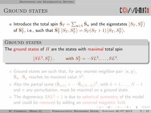
Introduce the total spin ST =∑
x∈Λ Sx and the eigenstates∣∣ST , S3
T
⟩of S2
T , i.e., such that S2T
∣∣ST , S3T
⟩= ST (ST + 1)
∣∣ST , S3T
⟩.
Ground statesThe ground states of H are the states with maximal total spin∣∣SL3, S3
T
⟩, with S3
T = −SL3, . . . , SL3.
Ground states are such that, for any nearest neighbor pair 〈x,y〉,Sx · Sy reaches its maximal value S2.
Also the partial sums (Sσ(1) + · · · Sσ(N−k))2, with k = 1, . . . , N − 1
and σ any perturbation, must be maximal on a ground state.The degeneracy 2SL3 + 1 is due to spherical symmetry of the modeland could be removed by adding an external magnetic field.
M. Correggi (Roma 3) Ferromagnetic Heisenberg Model Santiago 28/07/2015 5 / 15
Motivations and Mathematical Setting
Ground states
Introduce the total spin ST =∑
x∈Λ Sx and the eigenstates∣∣ST , S3
T
⟩of S2
T , i.e., such that S2T
∣∣ST , S3T
⟩= ST (ST + 1)
∣∣ST , S3T
⟩.
Ground statesThe ground states of H are the states with maximal total spin∣∣SL3, S3
T
⟩, with S3
T = −SL3, . . . , SL3.
Ground states are such that, for any nearest neighbor pair 〈x,y〉,Sx · Sy reaches its maximal value S2.
Also the partial sums (Sσ(1) + · · · Sσ(N−k))2, with k = 1, . . . , N − 1
and σ any perturbation, must be maximal on a ground state.The degeneracy 2SL3 + 1 is due to spherical symmetry of the modeland could be removed by adding an external magnetic field.
M. Correggi (Roma 3) Ferromagnetic Heisenberg Model Santiago 28/07/2015 5 / 15

Motivations and Mathematical Setting
Excited states: spin-waves
Assume that the system is in the ground state∣∣SL3, SL3
⟩(e.g.,
because of a small h < 0) =⇒ one can think of producing an excitedstate by lowering just one spin: setting S±x = S1
x ± iS2x,
|x〉 = 1√2SS−x∣∣SL3, SL3
⟩|x〉 is not an eigenstate of H but a linear combination can be...
Spin wavesThe spin waves are the orthonormal states (with k ∈ Λ∗ = 2π
L Z3)
|k〉 =1
L3/2
∑x∈Λ
eik·x |x〉
H |k〉 = Sε(k) |k〉 , ε(k) = 2∑
(1− cos ki) .
M. Correggi (Roma 3) Ferromagnetic Heisenberg Model Santiago 28/07/2015 6 / 15
Motivations and Mathematical Setting
Spin-wave approximation
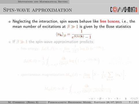
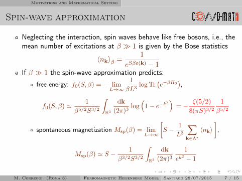
Neglecting the interaction, spin waves behave like free bosons, i.e., themean number of excitations at β � 1 is given by the Bose statistics
〈nk〉β =1
eSβε(k) − 1If β � 1 the spin-wave approximation predicts:
free energy: f0(S, β) = − limL→∞
1
βL3log Tr
(e−βH0
),
f0(S, β) ' 1
β
∫[−π,π]3
dk
(2π)3log(
1− e−βSε(k))' − ζ(5/2)
8(πS)3/2
1
β5/2
spontaneous magnetization Msp(β) = limL→∞
[S − 1
L3
∑k∈Λ∗
〈nk〉],
Msp(β) ' S −∫
[−π,π]3
dk
(2π)3
1
eSβε(k) − 1
M. Correggi (Roma 3) Ferromagnetic Heisenberg Model Santiago 28/07/2015 7 / 15

Motivations and Mathematical Setting
Spin-wave approximation
Neglecting the interaction, spin waves behave like free bosons, i.e., themean number of excitations at β � 1 is given by the Bose statistics
〈nk〉β =1
eSβε(k) − 1If β � 1 the spin-wave approximation predicts:
free energy: f0(S, β) = − limL→∞
1
βL3log Tr
(e−βH0
),
f0(S, β) ' 1
β
∫[−π,π]3
dk
(2π)3log(
1− e−βSε(k))' − ζ(5/2)
8(πS)3/2
1
β5/2
spontaneous magnetization Msp(β) = limL→∞
[S − 1
L3
∑k∈Λ∗
〈nk〉],
Msp(β) ' S −∫
[−π,π]3
dk
(2π)3
1
eSβε(k) − 1
M. Correggi (Roma 3) Ferromagnetic Heisenberg Model Santiago 28/07/2015 7 / 15

Motivations and Mathematical Setting
Spin-wave approximation
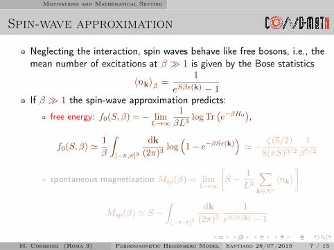
Neglecting the interaction, spin waves behave like free bosons, i.e., themean number of excitations at β � 1 is given by the Bose statistics
〈nk〉β =1
eSβε(k) − 1If β � 1 the spin-wave approximation predicts:
free energy: f0(S, β) = − limL→∞
1
βL3log Tr
(e−βH0
),
f0(S, β) ' 1
β5/2S3/2
∫R3
dk
(2π)3log(
1− e−k2)' − ζ(5/2)
8(πS)3/2
1
β5/2
spontaneous magnetization Msp(β) = limL→∞
[S − 1
L3
∑k∈Λ∗
〈nk〉],
Msp(β) ' S − 1
β3/2S3/2
∫R3
dk
(2π)3
1
ek2 − 1
M. Correggi (Roma 3) Ferromagnetic Heisenberg Model Santiago 28/07/2015 7 / 15
Motivations and Mathematical Setting
Spin-wave approximation
Neglecting the interaction, spin waves behave like free bosons, i.e., themean number of excitations at β � 1 is given by the Bose statistics
〈nk〉β =1
eSβε(k) − 1If β � 1 the spin-wave approximation predicts:
free energy: f0(S, β) = − limL→∞
1
βL3log Tr
(e−βH0
),
f0(S, β) ' 1
β5/2S3/2
∫R3
dk
(2π)3log(
1− e−k2)
= − ζ(5/2)
8(πS)3/2
1
β5/2
spontaneous magnetization Msp(β) = limL→∞
[S − 1
L3
∑k∈Λ∗
〈nk〉],
Msp(β) ' S − 1
β3/2S3/2
∫R3
dk
(2π)3
1
ek2 − 1
M. Correggi (Roma 3) Ferromagnetic Heisenberg Model Santiago 28/07/2015 7 / 15

Motivations and Mathematical Setting
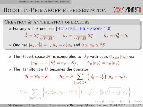
Holstein-Primakoff representation
Creation & annihilation operatorsFor any x ∈ Λ one sets [Holstein, Primakoff ‘40]
a†x = S+x
1√S−S3
x
, ax = 1√S−S3
x
S−x , nx = S3x + S,
One has [ax, a†x] = 1, nx = a†xax and 0 ≤ nx ≤ 2S.
The Hilbert space H is isomorphic to FS with basis ⊗x∈Λ |nx) via|nx)←→
∣∣S3x = nx − S
⟩, nx |nx) = nx |nx) .
The Hamiltonian H becomes the operator
H = H0 −K, H0 = S∑〈x,y〉⊂Λ
(a†x − a†y
)(ax − ay) ,
K =∑〈x,y〉⊂Λ
{a†xa
†yaxay − 2Sa†x
[1−
√1− nx
2S
√1− ny
2S
]ay
}.
M. Correggi (Roma 3) Ferromagnetic Heisenberg Model Santiago 28/07/2015 8 / 15

Motivations and Mathematical Setting
Holstein-Primakoff representation
Creation & annihilation operatorsFor any x ∈ Λ one sets [Holstein, Primakoff ‘40]
a†x = S+x
1√S−S3
x
, ax = 1√S−S3
x
S−x , nx = S3x + S,
One has [ax, a†x] = 1, nx = a†xax and 0 ≤ nx ≤ 2S.
The Hilbert space H is isomorphic to FS with basis ⊗x∈Λ |nx) via|nx)←→
∣∣S3x = nx − S
⟩, nx |nx) = nx |nx) .
The Hamiltonian H becomes the operator
H = H0 −K, H0 = S∑〈x,y〉⊂Λ
(a†x − a†y
)(ax − ay) ,
K =∑〈x,y〉⊂Λ
{a†xa
†yaxay − 2Sa†x
[1−
√1− nx
2S
√1− ny
2S
]ay
}.
M. Correggi (Roma 3) Ferromagnetic Heisenberg Model Santiago 28/07/2015 8 / 15

Motivations and Mathematical Setting
Validity of spin-wave approximation
H = S∑(
a†x − a†y)
(ax − ay)−K
The spin-wave approximation is given by dropping the spin-waveinteraction:
1 hard-core constraint nx ≤ 2S;2 attractive interaction K.
Physics of spin-wavesK is formally of relative size S−1 with respect to H0, so at least ifS � 1, the spin-wave approximation should be asymptotically correct.What if S is fixed and β →∞? spin-wave approximation is stillexpected to be correct! [Dyson ‘56; Zittartz ‘65].
M. Correggi (Roma 3) Ferromagnetic Heisenberg Model Santiago 28/07/2015 9 / 15

Motivations and Mathematical Setting
(math) Literature
Known resultsExactness of the spin-wave theory for the computation of the freeenergy, when S →∞ with β ∝ S−1 and a magnetic field h ∝ S[Conlon, Solovej ‘90].In the regime β →∞ with S fixed, there was only an upper bound tothe free energy (obtained through probabilistic methods) [Conlon,Solovej ‘91; Toth ‘93]
f0(1/2, β) ≤ C1
β5/2, with C1 > −
ζ(5/2)
(2π)3/2
where S is fixed equal to 1/2.Exactness of the spin-wave theory for the computation of the freeenergy when S →∞ with β ∝ S−1 [MC, Giuliani ’12].
M. Correggi (Roma 3) Ferromagnetic Heisenberg Model Santiago 28/07/2015 10 / 15

Main Results
Main result
Theorem (free energy [MC, Giuliani, Seiringer ‘13])
For any S ≥ 12 ,
limβ→∞
S3/2β5/2 f (S, β) =
∫R3
dk
(2π)3log(
1− e−k2)
= −ζ(5/2)
8π3/2
RemarksThe result is uniform in S for any finite S.In fact S needs not to be fixed but it is necessary that βS →∞,under the additional constraint βS � Sα.The upper bound proven in [Toth ‘93] was(
12
)3/2β5/2f(1/2, β) ≤ −ζ(5/2)
8π3/2log 2 + o(1)
M. Correggi (Roma 3) Ferromagnetic Heisenberg Model Santiago 28/07/2015 11 / 15
Main Results
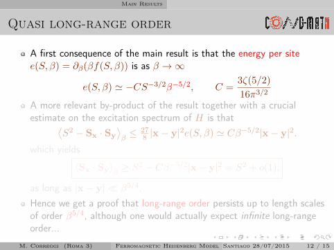
Quasi long-range order
A first consequence of the main result is that the energy per sitee(S, β) = ∂β(βf(S, β)) is as β →∞
e(S, β) ' −CS−3/2β−5/2, C =3ζ(5/2)
16π3/2
A more relevant by-product of the result together with a crucialestimate on the excitation spectrum of H is that⟨
S2 − Sx · Sy
⟩β≤ 27
8 |x− y|2e(S, β) ' Cβ−5/2|x− y|2.which yields
〈Sx · Sy〉β ≥ S2 − Cβ−5/2|x− y|2 = S2 + o(1),
as long as |x− y| � β5/4.Hence we get a proof that long-range order persists up to length scalesof order β5/4, although one would actually expect infinite long-rangeorder...
M. Correggi (Roma 3) Ferromagnetic Heisenberg Model Santiago 28/07/2015 12 / 15

Main Results
Quasi long-range order
A first consequence of the main result is that the energy per sitee(S, β) = ∂β(βf(S, β)) is as β →∞
e(S, β) ' −CS−3/2β−5/2, C =3ζ(5/2)
16π3/2
A more relevant by-product of the result together with a crucialestimate on the excitation spectrum of H is that⟨
S2 − Sx · Sy
⟩β≤ 27
8 |x− y|2e(S, β) ' Cβ−5/2|x− y|2.which yields
〈Sx · Sy〉β ≥ S2 − Cβ−5/2|x− y|2 = S2 + o(1),
as long as |x− y| � β5/4.Hence we get a proof that long-range order persists up to length scalesof order β5/4, although one would actually expect infinite long-rangeorder...
M. Correggi (Roma 3) Ferromagnetic Heisenberg Model Santiago 28/07/2015 12 / 15

Sketch of the Proof
Sketch of the proof
Upper bound1 Localization into boxes of side length `�
√β with Dirichlet b.c.;
2 Gibbs variational principle + trial state Γ = Pe−βH0P/norm., withP =
∏Px projecting onto hard-core states with nx ≤ 1.
3 Key estimate 1− P ≤ 12
∑nx (nx − 1) + Wick’s theorem.
Lower bound1 Localization into boxes of side length ` ∼
√β with Neumann b.c.;
2 Sharp lower bound on the excitation spectrumH ≥ C
`2
(S`3 − ST
)3 Preliminary lower bound on f(β) off the mark by log β =⇒ restriction
of the trace to states with small energy (few bosons!).
M. Correggi (Roma 3) Ferromagnetic Heisenberg Model Santiago 28/07/2015 13 / 15
Sketch of the Proof
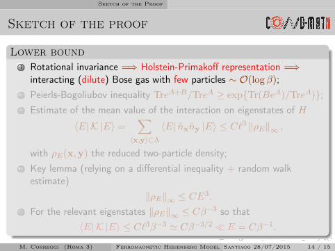
Sketch of the proof
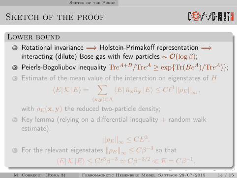
Lower bound4 Rotational invariance =⇒ Holstein-Primakoff representation =⇒
interacting (dilute) Bose gas with few particles ∼ O(log β);5 Peierls-Bogoliubov inequality TreA+B/TreA ≥ exp{Tr(BeA)/TreA)};6 Estimate of the mean value of the interaction on eigenstates of H
〈E| K |E〉 =∑〈x,y〉⊂Λ
〈E| nxny |E〉 ≤ C`3 ‖ρE‖∞ ,
with ρE(x,y) the reduced two-particle density;7 Key lemma (relying on a differential inequality + random walk
estimate)‖ρE‖∞ ≤ CE3.
8 For the relevant eigenstates ‖ρE‖∞ ≤ Cβ−3 so that〈E| K |E〉 ≤ C`3β−3 ' Cβ−3/2� E = Cβ−1.
M. Correggi (Roma 3) Ferromagnetic Heisenberg Model Santiago 28/07/2015 14 / 15
Sketch of the Proof
Sketch of the proof
Lower bound4 Rotational invariance =⇒ Holstein-Primakoff representation =⇒
interacting (dilute) Bose gas with few particles ∼ O(log β);5 Peierls-Bogoliubov inequality TreA+B/TreA ≥ exp{Tr(BeA)/TreA)};6 Estimate of the mean value of the interaction on eigenstates of H
〈E| K |E〉 =∑〈x,y〉⊂Λ
〈E| nxny |E〉 ≤ C`3 ‖ρE‖∞ ,
with ρE(x,y) the reduced two-particle density;7 Key lemma (relying on a differential inequality + random walk
estimate)‖ρE‖∞ ≤ CE3.
8 For the relevant eigenstates ‖ρE‖∞ ≤ Cβ−3 so that〈E| K |E〉 ≤ C`3β−3 ' Cβ−3/2� E = Cβ−1.
M. Correggi (Roma 3) Ferromagnetic Heisenberg Model Santiago 28/07/2015 14 / 15

Sketch of the Proof
Sketch of the proof
Lower bound4 Rotational invariance =⇒ Holstein-Primakoff representation =⇒
interacting (dilute) Bose gas with few particles ∼ O(log β);5 Peierls-Bogoliubov inequality TreA+B/TreA ≥ exp{Tr(BeA)/TreA)};6 Estimate of the mean value of the interaction on eigenstates of H
〈E| K |E〉 =∑〈x,y〉⊂Λ
〈E| nxny |E〉 ≤ C`3 ‖ρE‖∞,
with ρE(x,y) the reduced two-particle density;7 Key lemma (relying on a differential inequality + random walk
estimate)‖ρE‖∞ ≤ CE3.
8 For the relevant eigenstates ‖ρE‖∞ ≤ Cβ−3 so that〈E| K |E〉 ≤ C`3β−3 ' Cβ−3/2� E = Cβ−1.
M. Correggi (Roma 3) Ferromagnetic Heisenberg Model Santiago 28/07/2015 14 / 15

Sketch of the Proof
Sketch of the proof
Lower bound4 Rotational invariance =⇒ Holstein-Primakoff representation =⇒
interacting (dilute) Bose gas with few particles ∼ O(log β);5 Peierls-Bogoliubov inequality TreA+B/TreA ≥ exp{Tr(BeA)/TreA)};6 Estimate of the mean value of the interaction on eigenstates of H
〈E| K |E〉 =∑〈x,y〉⊂Λ
〈E| nxny |E〉 ≤ C`3 ‖ρE‖∞ ,
with ρE(x,y) the reduced two-particle density;7 Key lemma (relying on a differential inequality + random walk
estimate)‖ρE‖∞ ≤ CE3.
8 For the relevant eigenstates ‖ρE‖∞ ≤ Cβ−3 so that〈E| K |E〉 ≤ C`3β−3 ' Cβ−3/2� E = Cβ−1.
M. Correggi (Roma 3) Ferromagnetic Heisenberg Model Santiago 28/07/2015 14 / 15

Sketch of the Proof
Sketch of the proof
Lower bound4 Rotational invariance =⇒ Holstein-Primakoff representation =⇒
interacting (dilute) Bose gas with few particles ∼ O(log β);5 Peierls-Bogoliubov inequality TreA+B/TreA ≥ exp{Tr(BeA)/TreA)};6 Estimate of the mean value of the interaction on eigenstates of H
〈E| K |E〉 =∑〈x,y〉⊂Λ
〈E| nxny |E〉 ≤ C`3 ‖ρE‖∞ ,
with ρE(x,y) the reduced two-particle density;7 Key lemma (relying on a differential inequality + random walk
estimate)‖ρE‖∞ ≤ CE3.
8 For the relevant eigenstates ‖ρE‖∞ ≤ Cβ−3 so that〈E| K |E〉 ≤ C`3β−3 ' Cβ−3/2� E = Cβ−1.
M. Correggi (Roma 3) Ferromagnetic Heisenberg Model Santiago 28/07/2015 14 / 15

Sketch of the Proof
Thank you for the attention!
M. Correggi (Roma 3) Ferromagnetic Heisenberg Model Santiago 28/07/2015 15 / 15