Validation of FLUENT CFD model for hydrogen distribution in a

containment

D.C. Visser1 M. Houkema

N.B. Siccama1 E.M.J. Komen1

1Nuclear Research and Consultancy Group

Published in: Nuclear Engineering and Design 245 (2012) pp. 161-171

ECN-W--12-014 APRIL 2012

V

DN

a

ARRA

KHSCC

1

tTtitst

T

0d

Nuclear Engineering and Design 245 (2012) 161– 171

Contents lists available at SciVerse ScienceDirect

Nuclear Engineering and Design

j ourna l ho me page: www.elsev ier .com/ locate /nucengdes

alidation of a FLUENT CFD model for hydrogen distribution in a containment

.C. Visser ∗, M. Houkema1, N.B. Siccama, E.M.J. Komenuclear Research and Consultancy Group (NRG), Westerduinweg 3, 1755 ZG, Petten, The Netherlands

r t i c l e i n f o

rticle history:eceived 2 November 2011eceived in revised form 27 January 2012ccepted 30 January 2012

eywords:ydrogen stratificationevere accidentFDontainment thermal hydraulics

a b s t r a c t

Hydrogen may be released into the containment atmosphere of a nuclear power plant during a severeaccident. Locally, high hydrogen concentrations may be reached that can possibly cause fast deflagrationor even detonation and put the integrity of the containment at risk. The distribution and mixing ofhydrogen is, therefore, an important safety issue for nuclear power plants.

Computational fluid dynamics (CFD) codes can be applied to predict the hydrogen distribution in thecontainment within the course of a hypothetical severe accident and get an estimate of the local hydrogenconcentration in the various zones of the containment. In this way the risk associated with the hydrogensafety issue can be determined, and safety related measurements and procedures could be assessed. Inorder to further validate the CFD containment model of NRG in the context of hydrogen distributionin the containment of a nuclear power plant, the HM-2 test performed in the German THAI (thermal-hydraulics, hydrogen, aerosols and iodine) facility is selected. In the first phase of the HM-2 test a stratifiedhydrogen-rich light gas layer was established in the upper part of the THAI containment. In the secondphase steam was injected at a lower position. This induced a rising plume that gradually dissolved thestratified hydrogen-rich layer from below. Phenomena that are expected in severe accidents, like naturalconvection, turbulent mixing, condensation, heat transfer and distribution in different compartments,are simulated in this hypothetical severe accident scenario.

The hydrogen distribution and associated physical phenomena monitored during the HM-2 test arepredicted well by the CFD containment model. Sensitivity analyses demonstrated that a mesh resolutionof 45 mm in the bulk and 15 mm near the walls is sufficiently small to adequately model the hydrogendistribution and dissolution processes in the THAI HM-2 test. These analyses also showed that wall

functions could be applied. Sensitivity analyses on the effect of the turbulence model and turbulencesettings revealed that it is important to take the effect of buoyancy on the turbulent kinetic energy intoaccount. When this effect of buoyancy is included, the results of the standard k-ε turbulence model andSST k-ω turbulence model are similar and agree well with experiment. The outcome of these sensitivityanalyses can be used as input for setting up the guidelines on the application of CFD for containment issues.

. Introduction

During a severe accident in water-cooled reactors, large quan-ities of hydrogen and steam can be released into the containment.he hydrogen, generated as a result of core degradation and oxida-ion, can form a combustible gas mixture with the oxygen presentn the containment atmosphere. Unintended ignition of this mix-ure can initiate a combustion process, which may damage relevant

afety systems and challenge the integrity of the containment. Inhe worst-case, the safety function of the containment can get lost.

∗ Corresponding author. Tel.: +31 224 56 4193; fax: +31 224 56 8490.E-mail address: visser@nrg.eu (D.C. Visser).

1 Present address: Energy research Centre of the Netherlands (ECN), Petten,he Netherlands.

029-5493/$ – see front matter © 2012 Elsevier B.V. All rights reserved.oi:10.1016/j.nucengdes.2012.01.025

© 2012 Elsevier B.V. All rights reserved.

The potential danger of hydrogen was first realized after theThree Mile Island accident in 1979, where a large quantity of hydro-gen was released into the containment and started burning. Sincethen, many efforts have been taken to mitigate and/or reduce thepotential risk of hydrogen. For instance, by installation of hydrogenrecombiners that convert hydrogen to steam. The recent hydrogenexplosions during the Fukushima Daiichi accident in March 2011showed, however, that the control and mitigation of the hydrogenrisk is still a key safety issue for nuclear power plants.

In order to assess the potential risk of hydrogen and the effec-tiveness of the mitigation systems installed in the containment, itis necessary to predict the hydrogen concentration in the contain-ment during a severe accident. Two thermal-hydraulic approaches

can be used for this prediction (SOAR, 1999): the lumped parameter(LP) and the computational fluid dynamics (CFD) approach. The LPcodes are of practical use because they are able to give a quick esti-mate on the hydrogen distribution during a severe accident. The

162 D.C. Visser et al. / Nuclear Engineering

Nomenclature

Gb buoyancy effect source term (kg/m s3)g gravitational acceleration (m/s2)k turbulent kinetic energy (m2/s2)Prt turbulent Prandtl number (–)Re Reynolds number (–)

Greek symbolsε turbulent dissipation rate (m2/s3)� density (kg/m3)�t turbulent viscosity (kg/m s)ω specific dissipation rate (1/s)

hptoAaa

TyetiAdti(CtsnsPcce

ecwCapba

2Ouutsttt

tc

mercial general-purpose CFD package supplied by ANSYS Inc.

igh resolution CFD codes provide detailed information on localhenomena and concentrations. The OECD launched the interna-ional benchmark exercise ISP47 in order to assess the capabilitiesf both approaches for containment analyses (Allelein et al., 2007).

combined use of LP and CFD was recommended, where LP willct as the main workhorse and CFD will be used for more detailednalyses with high (local) resolution.

The 3D special purpose CFD codes GOTHIC, GASFLOW andONUS were the first CFD codes designed for containment anal-ses. GOTHIC is an EPRI-sponsored code that can be used forither lumped-parameter computations or for more detailed mul-idimensional analysis (Andreani and Paladino, 2010). GASFLOWs a joint development of Forschungszentrum Karlsruhe and Loslamos National Laboratory for the simulation of steam/hydrogenistribution and combustion in complex nuclear reactor con-ainment geometries (GASFLOW, 2011). TONUS is the Frenchn-house hydrogen risk analysis code developed by CEA and IRSNKudriakov et al., 2008). Compared to more recent commercialFD codes like CFX and FLUENT, these early codes are limited inheir meshing capabilities, turbulence modeling and multiproces-or parallel performance. Therefore the interest and use of theew, general purpose commercial codes for containment analy-es increased substantially over the last years (Heitsch et al., 2010;rabhudharwadkar et al., 2011). The GOTHIC, GASFLOW and TONUSodes are, however, still readily employed because of their spe-ific models (e.g. steam condensation and hydrogen mitigation) andxtensive validation.

Although the CFD codes have proven to be a powerful tool,xtensive validation and clear guidelines are necessary before theseodes can be reliably used for real plant analyses. In the presentork, the containment model developed by NRG in the commercialFD code FLUENT is further validated using the well instrumentednd well defined THAI HM-2 test. This test simulates the relevanthysical phenomena involved in the context of hydrogen distri-ution in a large, multi-compartment containment under severeccident conditions (Kanzleiter and Fischer, 2008).

The international benchmark exercise ISP47 (Allelein et al.,007) as well as the HM-2 benchmark exercise within theECD-NEA THAI project (Schwarz et al., 2010) showed a strongser-dependence, which demonstrates the importance of settingp and applying best practice guidelines (BPGs) specific for con-ainment applications. To make a start with the development ofuch BPGs, sensitivity analyses are performed in the present worko analyse the effect of mesh resolution, near-wall treatment,urbulence modeling and turbulence settings on the hydrogen dis-ribution in a containment.

The work presented here is part of NRG’s program on the longerm development and validation of a reliable and complete CFDontainment model for hydrogen distribution and combustion,

and Design 245 (2012) 161– 171

including mitigation systems such as recombiners, sprays, and con-densers.

2. THAI HM-2 experiment

The THAI facility is operated by Becker Technologies inEschborn, Germany. The objective of the HM (hydrogen mixing) testseries within the OECD-NEA THAI project was to study hydrogenmixing and distribution in a large, multi-compartment contain-ment. Test HM-1 was performed with inert helium gas and testHM-2 with hydrogen gas. A detailed description and comparisonof the HM tests is given by Gupta et al. (2010). The configuration ofthe THAI facility, instrumentation and test conditions of the HM-2experiment are specified by Kanzleiter and Fischer (2008).

Fig. 1 shows the THAI vessel with the internal structures asemployed in the HM tests. The THAI vessel is a cylindrical con-tainment with a height of 9.2 m, a diameter of 3.2 m and a totalvolume of 60 m3. The HM test setup facilitates the study of hydro-gen mixing in a multi-compartment facility: the vessel contains aninner cylinder and four condensate trays that divide the vessel intoa base, a cylinder, an annulus and a dome region. These differentcompartments in the THAI vessel are indicated in the schematicdrawing in Fig. 1. The inner cylinder with a height of 4 m and adiameter of 1.4 m is open at both ends. The condensate trays atan elevation of 4 m from the bottom of the vessel block 2/3 ofthe cross-sectional area in the annulus. Various instrumentationdevices are installed at different locations in the vessel for measur-ing the hydrogen concentration, temperature, pressure and flowvelocity.

At the start of the HM-2 test, the vessel atmosphere consistsof 98 vol% nitrogen gas, 1 vol% oxygen and 1 vol% steam at ambi-ent conditions (1 bar, 21 ◦C). The HM-2 test can be divided in twophases;

• Phase-1: hydrogen/steam injection and formation of a stablestratified hydrogen-rich gas layer in the upper part of the vessel(0–4300 s).• Phase-2: steam injection, dissolution of the stratified hydrogen-

rich gas layer and mixing of the atmosphere in the vessel(4300–6860 s).

In phase-1, a mixture of hydrogen (∼0.3 g/s) and saturated steam(∼0.24 g/s) is injected in upward direction into the annulus from acircular pipe of 28.5 mm diameter at an elevation of 4.8 m. The aver-age injection temperature during this phase is 45 ◦C. At the end ofphase-1, from 4200 to 4300 s, there is no injection. In phase-2, sat-urated steam (∼24 g/s) is injected in upward direction below thecentre of the inner cylinder from a nozzle of 138 mm diameter atan elevation of 1.8 m. The average injection temperature duringphase-2 is 108 ◦C. Detailed injection rates and injection tempera-tures during phase-1 and phase-2 of the HM-2 test are shown inFig. 2. Physical phenomena like convection, turbulent mixing, con-densation, heat transfer and distribution of gasses into differentcompartmens are simulated in these phases of the HM-2 test. Thesephenomena can be very relevant in the course of a severe accident.

3. CFD model

3.1. Introduction

The transient calculations are performed with FLUENT, a com-

In all calculations, one half of the THAI vessel is modeled,assuming symmetry across the vertical plane through the ves-sel axis. Since isotropic Reynolds averaged Navier-Stokes (RANS)

D.C. Visser et al. / Nuclear Engineering and Design 245 (2012) 161– 171 163

Fig. 1. THAI vessel configuration during the HM tests. On the left a three dimensional reprerepresentation showing the compartments and injection points.

Fig. 2. Injection rates and injection temperatures during phase-1 (top) and phase-2(bottom) of the THAI HM-2 test (Kanzleiter and Fischer, 2008).

sentation of the THAI vessel with internal structures. On the right a two-dimensional

turbulence models are applied, it is expected that this geomet-rical simplification have no effect as has been verified by Roylet al. (2009). The modeled three-dimensional geometry is shownin Fig. 3.

The solid walls and solid internal structures of the THAI ves-sel are modeled to take into account the effect of heat conduction

and heat capacity. Geometrical information and thermal propertiesof the solids are taken from Fischer (2004). The fluid in the ves-sel is modeled as a composition and temperature dependent ideal

Fig. 3. Three-dimensional geometry applied in the CFD calculations; one symmet-rical half of the THAI vessel.

164 D.C. Visser et al. / Nuclear Engineering and Design 245 (2012) 161– 171

Table 1General features of the CFD model.

Code version FLUENT 6.3

Solver Pressure-based segregatedFormulation TransientTurbulence approach RANSPressure interpolation scheme Body-force weightedPressure correction scheme PISOSpatial discretization 2nd Order upwindTemporal discretization 2nd Order implicitGeometry 3-Dimensional, half vesselWalls No slipNear-wall treatment Enhanced wall treatmentConduction 3-dimensionalFluid properties Composition and temperature

dependent ideal gasCondensation User-defined function, NRG

condensation modelTime step size Increases from 0.1 s (at the start of

gacltooT

(Cmadi(dtf

3

t

1234

w

H

woioTtmbmI

Table 2Initial conditions for the CFD calculations.

Pressure 1.008 bar

Temperature Linear temperature increase from18.6 ◦C at the bottom to 23.3 ◦C atthe top of the THAI vessel.

Composition 99 vol% nitrogen (1 vol% oxygen isneglected) 1 vol% steam

Velocity u, v, w = 0 m/s (fluid initially at rest)

each phase) to 0.2 s (after 20 s from thestart of each phase)

as mixture of its constituent components (nitrogen, hydrogennd steam). The temperature dependence of specific heat, thermalonductivity and viscosity is implemented by means of a piecewise-inear approach for each of the individual gas components. Theemperature dependent data for nitrogen, hydrogen and steam arebtained from Lemmon et al. (2007). Also the diffusion coefficientsf the components depend on gas composition and temperature.he effect of the 1 vol% oxygen initially present is neglected.

In general, the guidelines given in the FLUENT 6.3 User’s Guide2006) and by ERCOFTAC (2000) are followed for setting up theFD model. An overview of the general features of the applied CFDodel is given in Table 1. A condensation model was developed

nd used by NRG, since there are no models for wall and bulk con-ensation available in FLUENT. These condensation processes are

ncorporated in the CFD model by means of user-defined functionsUDF) referred to as the NRG Condensation Model. The NRG Con-ensation Model, the initial and boundary conditions as well ashe applied meshes and turbulence models are described in theollowing subsections.

.2. NRG condensation model

The implemented NRG Condensation Model takes into accounthe following processes:

. Bulk condensation and evaporation;

. Wall condensation;

. Deposition of bulk condensate on walls;

. Rainout of bulk condensate.

The condensation/evaporation process in the bulk and at theall is modeled by the reaction;

2O (g)kr←→ H2O (l) + heat,

here the reaction rate kr is controlled by the vapor pressure. Evap-ration of condensate from the walls is not expected and not takennto account. Furthermore, the water condensate that is depositedn the walls or rains out from the bulk is not treated in the model.he effect of this water condensate on for instance the flow, heat

ransfer and condensation is thus neglected. The NRG condensation

odel is described in more detail by Houkema et al. (2008) and haseen employed successfully in the SARNET Condensation Bench-ark (Ambrosini et al., 2007) and International Standard Problem

SP-47 on Containment Thermalhydraulics (Allelein et al., 2007).

Turbulence k, ε = 10−6 (low turbulenceassumed)

3.3. Initial and boundary conditions

The initial conditions for the THAI HM-2 test are specified byKanzleiter and Fischer (2008) and are adopted as starting pointof phase-1 in the calculations. The applied initial conditions arelisted in Table 2, where it must be noted that the linear temperatureincrease is applied for the solid walls as well.

Hydrogen and steam injection is modeled with mass-flow inletboundary conditions. The injection rates and injection tempera-tures during phase-1 and phase-2 of the HM-2 test are specified byKanzleiter and Fischer (2008) and are shown in Fig. 2. These timedependent boundary conditions are prescribed in tabular form inthe FLUENT CFD code. The turbulence quantities at the inlets arespecified in terms of turbulence intensity (I) and hydraulic diameter(Dh).

No-slip boundary conditions are imposed on the solid wallsand solid structures, using the enhanced wall treatment (EWT)approach in FLUENT to model the flow near the walls. The EWTis a near-wall modeling method that combines a two-layer modelwith (enhanced) wall functions. If the near-wall mesh is fine enough(typically y+≈ 1), the EWT will automatically resolve the laminarsublayer. In all other cases, the EWT will automatically make useof wall-functions. A similar approach is followed for modeling thenear-wall heat and species transport. The vessel’s outer wall isinsulated and assumed adiabatic. All other walls are modeled asfluid-solid interfaces with conjugate heat-transfer. Heat transferby means of radiation is neglected. Condensation takes place on allthe walls that are in contact with the gas mixture inside the vessel.

3.4. Computational mesh

Four different computational meshes are constructed in order tostudy the effect of mesh resolution and near-wall treatment (two-layer model or wall-functions). The four meshes are constructedin a similar way. Table 3 presents the characteristics of the fourmeshes. Fig. 4 shows the “standard” mesh. The solid regions arefilled with hexahedral cells. The fluid regions consist of a hybridmesh with tetrahedral and hexahedral cells. The vessel’s baseregion is mostly filled with unstructured tetrahedral mesh cells.The annulus, cylinder and dome region consist of structured andunstructured hexahedral cells. The mesh is refined towards thewalls and solid structures in order to resolve the flow and physicalphenomena near the wall in more detail. The mesh at and abovethe inlets is refined in order to resolve the small inflow area andthe injection jet in more detail.

The characteristics of the four meshes are listed in Table 3. Inthe y+ = 1 mesh, the typical cell size is 0.25 mm near the walls and30 mm × 50 mm in the bulk. In the standard, coarse and fine meshthe typical cell size is 15 mm near the walls and 30 mm × 50 mm,45 mm × 75 mm and 20 mm × 30 mm in the bulk, respectively.

Fig. 5 compares the four meshes at a section near the inner cylinder.Depending on the mesh resolution and the flow properties nearthe wall, the EWT approach in FLUENT makes use of wall func-tions or resolves the viscous boundary layer at the wall. The small

D.C. Visser et al. / Nuclear Engineering and Design 245 (2012) 161– 171 165

Table 3Constructed computational meshes.

Mesh y+ = 1 mesh Standard mesh Coarse mesh Fine mesh

Total number of cells 763.905 543.438 175.069 2562.528Number of fluid cells 671.225 453.158 139.160 2197.401Typical cell size in the bulk (radial × vertical direction) 30 mm × 50 mm 30 mm × 50 mm 45 mm × 75 mm 20 mm × 30 mmTypical cell size at the wall 0.25 mm 15 mm 15 mm 15 mmTypical y+ ≤1 5–20 5–20 5–20Near-wall treatment Two-layer model Wall functions Wall functions Wall functions

Fig. 4. Front view of the standard mesh on the vessel’s symmetry plane (left) andtop view of the standard mesh on the horizontal cross section through the hydrogeninlet at y = 4.8 m (right). The mesh at the hydrogen inlet is shown in more detail forSections 1 and 3. The inflow area is filled/colored. The mesh resolution near the wallof the inner cylinder (Section 2) is shown in more detail for the four different meshesin Fig. 5.

Fig. 5. Top view of the four constructed meshes at the wall of the inner cylinder(Section 2 in Fig. 4).

Table 4Considered turbulence settings.

Case Turbulencemodel

Buoyancy effect included in

1 (reference case) SKE k and ( (full buoyancy option)2 SKE k (by default)3 SKW None (by default)4 SKW k (by UDF)

5 SSTKW None (by default)6 SSTKW k (by UDF)

near-wall cells in the y+ = 1 mesh make it possible to resolve theviscous boundary layer near the walls (y+ ≤ 1). Wall functions willbe applied in most near-wall regions for the standard, coarse andfine mesh (y+ > 1).

3.5. Turbulence model

In general, the standard k-ε turbulence model (SKE) with fullbuoyancy effects and default turbulent constants is utilized for theCFD analyses in this paper (i.e. the reference case). In order to studythe effect of the turbulence model and the buoyancy effects, the cal-culation for phase-2 of the HM-2 test is repeated using the standardk-ω (SKW) and the SST k-ω turbulence model (SSTKW) with andwithout taking into account the effect of buoyancy on turbulence.An overview of the considered cases is given in Table 4. This sensi-tivity study on turbulence settings is performed on the coarse mesh.It will be demonstrated in the next chapter that the resolution ofthe coarse mesh suffices to capture the relevant flow phenomenain the HM-2 test.

The k-ε models as well as the k-ω models belong to the classof two-equation RANS turbulence models. In the k-ε models tur-bulence is modeled with the transport equation for the turbulentkinetic energy (k) and its dissipation rate (ε). In the k-ω models tur-bulence is modeled with the transport equation for the turbulentkinetic energy (k) and the specific dissipation rate (ω). The standardk-ω model in FLUENT is based on the Wilcox k-ω model. The SSTk-ω model is developed by Menter (1994) and combines the best ofthe k-ε and k-ω formulations, blending the robust and accurate k-ωformulation in the near-wall region with the reliable k-ε formula-tion in the bulk region. A detailed description of the k-ε and k-ωturbulence models is given in the FLUENT 6.3 User’s Guide (2006).

In a non-zero gravity field, buoyancy forces can suppress or pro-mote turbulence in the presence of density gradients. Buoyancytends to suppress turbulence at a stable stratification and buoyancypromotes turbulence at an unstable stratification. The production(or dissipation) of turbulence by buoyancy can be incorporated inthe k-ε and k-ω turbulence models by adding the source term Gb tothe transport equation for k. The source term Gb is defined as

Gb = −gy�t

�Prt

∂�

∂y,

where y is the vertical direction, gy the gravitational accelerationin the y-direction, �t the turbulent viscosity, � the density and Prt

the turbulent Prandtl number. In FLUENT, Gb is only included bydefault in the k-equation of all the k-ε models. It is however possible

1 ering and Design 245 (2012) 161– 171

tm

itoacoF

4

anrw

we

4

gatpapmooo

ltbTtth1camamtca

itat

Therefore, under-prediction of condensation could be a possiblereason for the observed deviation in pressure and hydrogen con-centration between the CFD calculation and the experiment. This

66 D.C. Visser et al. / Nuclear Engine

o incorporate Gb in the k-equation of the k-ω models as well byeans of a ‘so called’ user-defined function (UDF).Since the effect of buoyancy on the turbulent dissipation rate ε

s not well understood, by default this effect is not included in theransport equation for ε in FLUENT (FLUENT, 2006). A certain effectf buoyancy on ε can be included in the k-ε models of FLUENT byctivating the “full buoyancy” option. The effect of buoyancy on εan be observed by comparison of cases 1 and 2 in Table 4. The effectf buoyancy is not included in the ω-equation of the k-ω models inLUENT and is therefore not considered here.

. Results

In this chapter, the results of the CFD analyses are presentednd compared to the HM-2 experiment performed by Becker Tech-ologies (EXPBT). The results of the sensitivity analyses on meshesolution and turbulence models/settings are presented here asell. This chapter is divided into the following sections:

Section 4.1: comparison of the experimental and CFD results forphase-1.Section 4.2: comparison of the experimental and CFD results forphase-2.Section 4.3: effect of mesh resolution and near-wall treatment.Section 4.4: effect of turbulence model and buoyancy effects.

The CFD results presented in Sections 4.1 and 4.2 are obtainedith the standard k-ε turbulence model (SKE) with full buoyancy

ffects on the y+ = 1 mesh.

.1. Phase-1 results (0–4300 s)

In phase-1 of the HM-2 test, a total amount of 1.24 kg hydro-en and 1 kg saturated steam is injected into the THAI vessel from

vertical pipe in the annulus. Since the THAI vessel is closed,he hydrogen and steam content will increase, and therewith theressure as well. The measured and calculated evolution of thetmospheric pressure and hydrogen mass in the vessel duringhase-1 is shown in Fig. 6. The CFD calculation shows an accurateass balance and a negligible error of less than 0.2% in the amount

f hydrogen in the system. The calculation shows, however, a slightver-prediction of the vessel pressure (about 0.02 bars at the endf phase-1).

The injected gas mixture of hydrogen and steam has a relativelyow density and forms a stable stratified hydrogen-rich gas layer inhe upper part of the THAI vessel. Fig. 7 shows the hydrogen distri-ution at the end of phase-1 on a vertical line through the annulus.he experiment and calculation show a similar hydrogen distribu-ion in the THAI vessel. Initially the vessel contains no hydrogen. Athe end of phase-1, a hydrogen-rich gas layer is formed in the upperalf of the vessel, while the hydrogen concentration remains below% in the lower half of the vessel. A strong gradient in hydrogen con-entration is observed at an elevation of 4–5 m. The inset in Fig. 7 is

contour plot of the predicted hydrogen concentration on the sym-etry plane at 4300 s. This contour clearly shows that the hydrogen

ccumulates and is well mixed in the upper half of the vessel. Theeasured and predicted values of the hydrogen concentration in

he hydrogen-rich gas layer differ slightly. In the experiment, con-entrations up to 37 vol% are found in the upper part of the vessel,gainst concentrations up to 35.5 vol% in the calculation.

During phase-1, a mixture of hydrogen and saturated steam is

njected at an average temperature of 45 ◦C. The temperature ofhe gas and the solid structures in the vessel is lower, which causesbout 50% of the injected steam to condensate in the CFD calcula-ion. Condensation of steam lowers the pressure in the vessel and

Fig. 6. Comparison of the measured (EXPBT) and predicted (CFD) atmospheric pres-sure (top) and amount of hydrogen (bottom) in the vessel during phase-1.

increases the concentration of the other species in the gas mixture.

Fig. 7. Comparison of the measured (EXPBT) and predicted (CFD) hydrogen concen-tration at the end of phase-1 on a vertical line running through the annulus fromthe bottom to the top of the THAI vessel (see dashed line in inset). The inset showsa contour plot of the predicted hydrogen concentration on the symmetry plane atthe end of phase-1.

ering and Design 245 (2012) 161– 171 167

eicmchs(bilsglAhtcaea

4

ttisplpiC6oi

ttipesp

st2oflte4t04Cestv

fea

illustrate and understand the processes during phase-2. As shownin Figs. 9 and 10, the hydrogen concentration in the upper partof the vessel is uniformly high at the start of phase-2, while it is

D.C. Visser et al. / Nuclear Engine

ffect of condensation and its importance in the THAI HM-2 tests also demonstrated by Royl et al. (2009). Under-prediction ofondensation can have different causes, for instance the imple-ented condensation model, the imposed initial conditions (gas

omposition and temperature distribution) and/or the modeledeat transfer to the solids. The influence of the heat losses to theolids for the THAI HM-2 test is also considered by Schwarz et al.2010) and Bentaib and Bleyer (2011). This heat transfer effect cane understood by observing the temperatures of the gas mixture

n the vessel. The predicted gas temperature in the hydrogen-richayer in the upper part of the vessel is about 1 ◦C higher than mea-ured in the experiment, which indicates that heat transfer from theas to the solids is slightly under-predicted. At higher temperature,ess steam will condensate from the humid, hydrogen-rich layer.t the end of phase-1, the predicted steam concentration in theydrogen-rich layer is still around 2 vol%. Since limited experimen-al data is available on the steam distribution in the vessel, a directomparison to the measured steam concentrations cannot be madend no conclusive explanation can be given for the observed differ-nces in pressure and hydrogen concentration between calculationnd experiment.

.2. Phase-2 results (4300–6860 s)

In phase-2 of the HM-2 test, saturated steam at relatively highemperature is injected into the THAI vessel from a nozzle belowhe centre of the inner cylinder. The injected steam first clears thenner cylinder and then starts to dissolve the stable hydrogen-richtratification in the vessel dome from below. These two consecutiverocesses divide phase-2 into a stagnation and a natural circu-

ation period. The point in time where this “natural circulationeriod” starts is referred to as the onset of natural circulation. Dur-

ng phase-2 the amount of steam in the vessel, as predicted by theFD calculation, increases from 1 kg at 4300 s to 6 kg at 6500 s. At500 s the amount of steam injected is ∼53 kg, which means thatver 90% of the injected steam condensates. Condensation of steams, thus, very important during phase-2.

The predicted atmospheric pressure and flow velocity abovehe centre of the inner cylinder during phase-2 are compared tohe experimental results in Fig. 8. A vertical dashed line is drawnn the figures at 4300 s and at 4820 s, which indicate the start ofhase-2 and the onset of natural circulation as determined fromxperiment, respectively. The period from 4300 s to 4820 s is thetagnation period. The period after 4820 s is the natural circulationeriod.

Fig. 8 shows that the measured and predicted evolution of pres-ure follow the same trend. The over-prediction in pressure athe end of phase-1 remains more or less constant during phase-. Fig. 8 also compares the vertical flow velocity above the centref the inner cylinder during phase-2. The measured and predictedow velocity agree well on average, and fluctuations have abouthe same amplitude. The start of the natural circulation period isvident by the sudden significant increase in flow velocity around800 s. When the onset of natural circulation is determined as theime when the flow velocity above the inner cylinder stays above.15 m/s, the onset found from experiment and CFD is 4820 s and720 s, respectively. The earlier onset of natural circulation in theFD calculation are expected to be the result of the slightly differ-nt starting conditions for phase-2 compared to the experiment. Aecond increase in flow velocity is observed around 6000 s whenhe hydrogen-rich gas layer is almost completely dissolved. Theelocity drops to zero when the injection of steam is stopped.

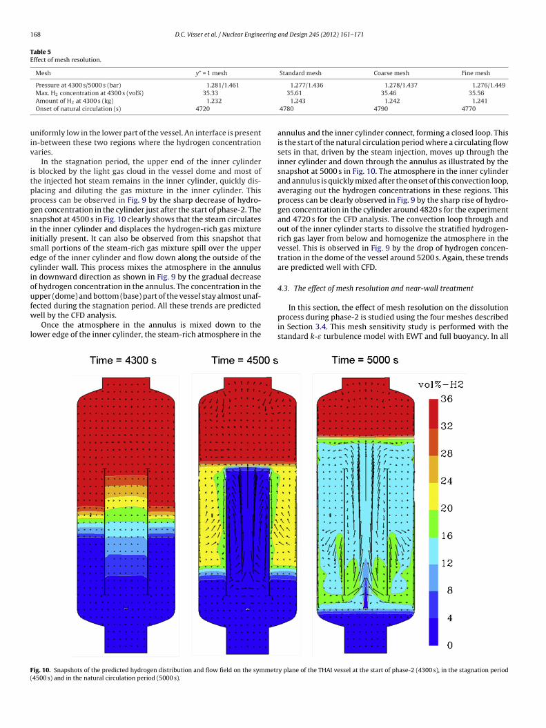
Fig. 9 compares the hydrogen concentration during phase-2 atour different locations in the vessel. Each location is in a differ-nt compartment of the vessel (base, annulus, cylinder and dome)s shown in the insets in Fig. 9. Fig. 10 shows snapshots of the

Fig. 8. Atmospheric pressure (top) and vertical flow velocity above the centre ofthe inner cylinder (bottom) during phase-2. The experiment ends at 6860 s, thecalculation runs up to 6500 s.

predicted hydrogen distribution and flow field on the symmetryplane at 4300 s, 4500 s and 5000 s. These snapshots are helpful to

Fig. 9. Hydrogen concentrations in the vessel during phase-2 as measured (symbols)and computed (solid lines) for the THAI HM-2 test.

168 D.C. Visser et al. / Nuclear Engineering and Design 245 (2012) 161– 171

Table 5Effect of mesh resolution.

Mesh y+ = 1 mesh Standard mesh Coarse mesh Fine mesh

Pressure at 4300 s/5000 s (bar) 1.281/1.461 1.277/1.436 1.278/1.437 1.276/1.449

uiv

itppgsiisecioufw

l

F(

Max. H2 concentration at 4300 s (vol%) 35.33

Amount of H2 at 4300 s (kg) 1.232

Onset of natural circulation (s) 4720

niformly low in the lower part of the vessel. An interface is presentn-between these two regions where the hydrogen concentrationaries.

In the stagnation period, the upper end of the inner cylinders blocked by the light gas cloud in the vessel dome and most ofhe injected hot steam remains in the inner cylinder, quickly dis-lacing and diluting the gas mixture in the inner cylinder. Thisrocess can be observed in Fig. 9 by the sharp decrease of hydro-en concentration in the cylinder just after the start of phase-2. Thenapshot at 4500 s in Fig. 10 clearly shows that the steam circulatesn the inner cylinder and displaces the hydrogen-rich gas mixturenitially present. It can also be observed from this snapshot thatmall portions of the steam-rich gas mixture spill over the upperdge of the inner cylinder and flow down along the outside of theylinder wall. This process mixes the atmosphere in the annulusn downward direction as shown in Fig. 9 by the gradual decreasef hydrogen concentration in the annulus. The concentration in thepper (dome) and bottom (base) part of the vessel stay almost unaf-

ected during the stagnation period. All these trends are predictedell by the CFD analysis.

Once the atmosphere in the annulus is mixed down to theower edge of the inner cylinder, the steam-rich atmosphere in the

ig. 10. Snapshots of the predicted hydrogen distribution and flow field on the symmetr4500 s) and in the natural circulation period (5000 s).

35.61 35.46 35.561.243 1.242 1.241

4780 4790 4770

annulus and the inner cylinder connect, forming a closed loop. Thisis the start of the natural circulation period where a circulating flowsets in that, driven by the steam injection, moves up through theinner cylinder and down through the annulus as illustrated by thesnapshot at 5000 s in Fig. 10. The atmosphere in the inner cylinderand annulus is quickly mixed after the onset of this convection loop,averaging out the hydrogen concentrations in these regions. Thisprocess can be clearly observed in Fig. 9 by the sharp rise of hydro-gen concentration in the cylinder around 4820 s for the experimentand 4720 s for the CFD analysis. The convection loop through andout of the inner cylinder starts to dissolve the stratified hydrogen-rich gas layer from below and homogenize the atmosphere in thevessel. This is observed in Fig. 9 by the drop of hydrogen concen-tration in the dome of the vessel around 5200 s. Again, these trendsare predicted well with CFD.

4.3. The effect of mesh resolution and near-wall treatment

In this section, the effect of mesh resolution on the dissolutionprocess during phase-2 is studied using the four meshes describedin Section 3.4. This mesh sensitivity study is performed with thestandard k-ε turbulence model with EWT and full buoyancy. In all

y plane of the THAI vessel at the start of phase-2 (4300 s), in the stagnation period

D.C. Visser et al. / Nuclear Engineering and Design 245 (2012) 161– 171 169

Fbl

cs

ttathsvtrtamem

obo

Ftl

ig. 11. Comparison of the measured hydrogen concentrations in the vessel (sym-ols) with those computed on the y+ = 1 mesh (solid lines) and standard mesh (dotted

ines).

alculations the convergence was in the order of 10−5 for flow andpecies, and in the order of 10−9 for energy.

The y+ = 1 and standard mesh have the same mesh resolution inhe bulk and a different mesh resolution near the wall. To assesshe effect of near-wall treatment, the results obtained on the y+ = 1nd standard mesh are compared qualitatively in Fig. 11 and quan-itatively in Table 5. Fig. 11 shows again the development of theydrogen concentration over time at the four locations in the ves-els’ base, annulus, cylinder and dome compartment. Table 5 showsalues of pressure, hydrogen concentration, mass conservation andhe time of onset of natural circulation for the different meshes. Theesults obtained on the standard mesh with wall functions and onhe y + =1 mesh with the two-layer model are very similar. The over-ll mixing process during phase-2 is slightly slower for the standardesh. Nevertheless, the results agree well and are both close to the

xperimental results, meaning that wall functions are applicable toodel the THAI HM-2 test.

The standard, coarse and fine mesh have the same mesh res-

lution near the wall and a different mesh resolution in theulk (see Table 3). The effect of bulk mesh resolution can bebserved in Fig. 12 and Table 5, where the results obtained on the

ig. 12. Comparison of the hydrogen concentrations in the vessel as computed onhe standard mesh (solid line), coarse mesh (broken line), and fine mesh (dottedine).

Fig. 13. Hydrogen concentrations in the vessel atmosphere during phase-2 as mea-sured (EXPBT) and computed with different turbulence models and buoyancy terms.

170 D.C. Visser et al. / Nuclear Engineering and Design 245 (2012) 161– 171

F I vessG ut Gb

sss

4

ttTts2w(

vtcertmmowhtveb

ig. 14. Snapshots of the hydrogen distribution on the symmetry plane of the THAb), the SST k-ω turbulence model with Gb and the SST k-ω turbulence model witho

tandard, coarse and fine mesh are compared. The differences aremall, which shows that a cell size of 45 mm ×75 mm in the bulk isufficiently small to model the THAI HM-2 test.

.4. The effect of turbulence model

In this section, the effects of the turbulence model and buoyancyerms in the turbulence models on the prediction of the dissolu-ion process during phase-2 are studied for the settings given inable 4. All analyses are performed on the coarse mesh. Apart fromhe turbulence settings, the analyses are performed with the sameettings. In order to assure identical starting conditions for phase-, all calculations start at 4300 s on the phase-1 solution obtainedith the standard k-ε model with full buoyancy on the coarse mesh

case 1 in Table 4).Fig. 13 compares the computed hydrogen concentrations in the

essel atmosphere during phase-2 for the different turbulence set-ings listed in Table 4. The stagnation period and onset of naturalirculation is predicted reasonably well in all calculations. How-ver, compared to the experiment, the dissolution of the hydrogenich cloud sets in too early and the dissolution rate is higher forhe standard k-ω and SST k-ω models without Gb in k, as imple-

ented by default in FLUENT. The prediction of both these k-ωodels improves when Gb is included in the transport equation

f the turbulent kinetic energy k. Although the standard k-ω modelith Gb in k still predicts a slightly higher dissolution rate of theydrogen rich cloud compared to the experiment, the results of

he SST k-ω model with Gb agree well with experiment and areery similar to the results of the standard k-ε model with Gb. Appar-ntly, the generation (or dissipation) of turbulent kinetic energy byuoyancy has a large effect on the stability and dissolution process

el at 4500 s as predicted with the standard k-ε turbulence model (by default with.

of the stratified hydrogen-rich layer. This influence of buoyancy canbe understood as will be explained in the next paragraph. Includ-ing the buoyancy effect in the turbulent dissipation rate ε of thestandard k-ε model shows no significant influence.

Fig. 14 shows the hydrogen distribution on the symmetry planeat 4500 s as calculated with the standard k-ε model with Gb in k andε, the SST k-ω model with Gb in k and the SST k-ω model withoutGb. At 4500 s the HM-2 test is in the stagnation period of phase-2.In the experiment, the injected steam flows into the inner cylinderduring the stagnation phase without affecting the hydrogen con-centration in the dome area above the inner cylinder. As shown inFigs. 13 and 14, this is only true for the calculation with the standardk-ε turbulence model and the SST k-ω model with Gb. The snapshotsin Fig. 14 show that in the calculation of the SST k-ω model withoutGb, some of the steam flowed out of the inner cylinder and mixedwith the hydrogen rich cloud at 4500 s. This proves that it is impor-tant to take the effect of buoyancy into account in the turbulencemodel by including the Gb term. Turbulence is suppressed by buoy-ancy (Gb < 0) near the stratified hydrogen rich layer. Without thisdamping effect, the stratified layer above the inner cylinder will bedissolved faster by turbulent mixing. Consequently, the turbulencemodels without Gb do not correctly capture the dissolution processduring phase-2.

5. Conclusions

In the present work, the containment model of NRG is further

validated in the context of hydrogen distribution in a contain-ment using the THAI HM-2 test. For this test, the characteristicphenomena are the development and dissolution of a hydrogen-rich gas layer in the upper part of the THAI containment by a

ering

bcam

•

•

•

•

•

•

tptgttma

A

Ni

D.C. Visser et al. / Nuclear Engine

uoyant plume. These phenomena are predicted well by NRG’sontainment model developed in FLUENT. Additional sensitivitynalyses on mesh resolution, near-wall treatment, and turbulenceodel and turbulence model settings, showed the following:

A cell size of 45 mm × 75 mm in the bulk is sufficiently small tomodel the hydrogen distribution and dissolution processes in theTHAI HM-2 test with CFD.Good CFD results are obtained when wall functions are appliedto model the flow in the near wall region for the HM-2 test.The effect of buoyancy on the turbulent kinetic energy k is takeninto account by default in the k-ε turbulence models of FLUENT.This effect on k is not incorporated by default in the k-ω modelsof FLUENT, but it can be incorporated by user coding.The prediction of the dissolution process during phase-2 of theHM-2 test improves when the effect of buoyancy on k is includedin the turbulence models. Without this effect the CFD model pre-dicts a too early start of the dissolution, as well as a too highdissolution rate of the stratified hydrogen-rich layer.The results of the standard k-ε model and SST k-ω turbulencemodel with the effect of buoyancy on k included are very sim-ilar and agree well with experiment, whereas the standard k-ωturbulence model with the effect of buoyancy on k included stillpredicts a higher dissolution rate.The effect of buoyancy on the turbulent dissipation rate ε can beincluded in the k-ε models of FLUENT by activating the “full buoy-ancy” option. The buoyancy effect on ε is subject to discussion inliterature. For the HM-2 test, there was no significant impact onthe results obtained with CFD.

These findings, combined with the extensive model descrip-ion as presented in this paper may serve others in improving theredictive quality of CFD for containment analyses. Furthermore,hese findings and settings can develop into a set of best practiceuidelines for the application of CFD for containment analyses. Tohis end, more experimental tests should be analyzed in the futureo confirm the general applicability of the presented containment

odel and model settings. Work in this area is currently ongoingt NRG.

cknowledgments

The authors thank all signatories and participants to the OECD-EA THAI project. Special thanks are expressed to the people

nvolved in the experiments and documentation. In addition,

and Design 245 (2012) 161– 171 171

the authors gratefully acknowledge the funding provided by theDepartment of Nuclear Safety, Security and Safeguards (KFD) thatis presently part of the Dutch Ministry of Infrastructure and Envi-ronment.

References

Allelein, H.J., et al., 2007. International Standard Problem ISP-47 on ContainmentThermalhydraulics, Final Report. NEA/CSNI, OECD, Paris.

Ambrosini, W., et al., 2007. Results of the SARNET Condensation Benchmark No. 0.DIMNP 006(2007). University of Pisa.

Andreani, M., Paladino, D., 2010. Simulation of gas mixing and transport in a multi-compartment geometry using the GOTHIC containment code and relativelycoarse meshes. Nucl. Eng. Des. 240, 1506–1527.

Bentaib, A., Bleyer, A., 2011. ASTEC validation on OECD/THAI HM-2. In: Proceedingsof ICAPP’11, Nice, France, May 2–5, Paper 11258.

ERCOFTAC, 2000. Best Practice Guidelines, www.ercoftac.org.Fischer, K., 2004. International Standard Problem ISP-47 on Containment Thermal-

Hydraulics, Step 2: ThAI, Volume 1: Specification Report. Becker TechnologiesGmbH, Eschborn, Report No. BF-R 70031-1 Rev. 4.

FLUENT 6.3 User’s Guide, 2006. FLUENT Inc.GASFLOW, 2011. http://hycodes.net/gasflow.Gupta, S., Kanzleiter, T., Fischer, K., Langer, G., Poss, G., 2010. Interaction of a strati-

fied light gas layer with a buoyant jet in containment: hydrogen/helium materialscaling. In: Proceedings of ICAPP’10, San Diego, CA, USA, June 13–17, Paper10205.

Heitsch, M., Baraldi, D., Wilkening, H., 2010. Simulation of containment jet flowsincluding condensation. Nucl. Eng. Des. 240, 2176–2184.

Houkema, M., Siccama, N.B., Lycklama à Nijeholt, J.A., Komen, E.M.J., 2008. Validationof the CFX4 CFD code for containment thermal-hydraulics. Nucl. Eng. Des. 238,590–599.

Kanzleiter, T., Fischer, K., 2008. Quick Look Report Helium/Hydrogen Material Scal-ing Test HM-2. Becker Technologies GmbH, Eschborn, Germany, OECD-NEA THAIProject Report No. 150 1326 – HM-2 QLR Rev. 3.

Kudriakov, S., Dabbene, F., Studer, E., Beccantini, A., Magnaud, J.P., Paillère, H., Ben-taib, A., Bleyer, A., Malet, J., Porcheron, E., Caroli, C., 2008. The TONUS CFD codefor hydrogen risk analysis, physical models, numerical schemes and validationmatrix. Nucl. Eng. Des. 238, 551–565.

Lemmon, E.W., Huber, M.L., McLinden, M.O., 2007. NIST Standard ReferenceDatabase 23: Reference Fluid Thermodynamic and Transport Properties-REFPROP, Version 8. 0. National Institute of Standards and Technology, StandardReference Data Program, Gaithersburg.

Menter, F.R., 1994. Two-equation Eddy-viscosity turbulence models for engineeringapplications. AIAA J. 32 (8), 1598.

Prabhudharwadkar, D.M., Iyer, K.N., Mohan, N., Bajaj, S.S., Markandeya, S.G., 2011.Simulation of hydrogen distribution in an Indian nuclear reactor containment.Nucl. Eng. Des. 241, 832–842.

Royl, P., Travis, J.R., Breitung, W., Kim, J., Kanzleiter, T., Schwarz, S., 2009. GASFLOWanalysis of steam/hydrogen mixing with nitrogen in the OECD-NEA THAI HM-2benchmark. In: Proc. of NURETH-13, Kanazawa, Japan, September 27–October2, Paper N13P1412.

Schwarz, S., Fischer, K., Bentaib, A., Burkhardt, J., Lee, J.-J., Duspiva, J., Visser, D.,

Kyttala, J., Royl, P., Kim, J., Kostka, P., Liang, R., 2010. Benchmark on hydrogendistribution in a containment based on the OECD-NEA THAI HM-2 experiment.Nucl. Technol. 175, 594–603.

SOAR, 1999. SOAR on Containment Thermalhydraulics and Hydrogen Distribution,NEA/CSNI/R(1999)16.