Validation of a Wireless Sensor Network using Local Damage Detection algorithm for Beam-Column Connections

S. Dorvasha, S.N. Pakzada, E. Labuza, M. Changa, X. Lib, L. Chengb ,

aDept. of Civil and Environmental Engineering, Lehigh Univ., Bethlehem, PA USA bDept. of Computer Science and Engineering, Lehigh Univ., Bethlehem, PA USA

ABSTRACT

There has been a rapid advancement in wireless sensor network (WSN) technology in the past decade and its application in structural monitoring has been the focus of several research projects. The evaluation of the newly developed hardware platform and software system is an important aspect of such research efforts. Although much of this evaluation is done in the laboratories and using generic signal processing techniques, it is important to validate the system for its intended application as well. In this paper the performance of a newly developed accelerometer sensor board is evaluated by using the data from a beam-column connection specimen with a local damage detection algorithm. The sensor board is a part of a wireless node that consists of the Imote2 control/communication unit and an advanced antenna for improved connectivity. A scaled specimen of a steel beam-column connection is constructed in ATLSS center at Lehigh University and densely instrumented by synchronized networked systems of both traditional piezoelectric and wireless sensors. The column ends of the test specimen have fixed connections, and the beam cantilevers from the centerline of the column. The specimen is subjected to harmonic excitations in several test runs and its acceleration response is collected by both systems. The collected data is then used to estimate two sets of system influence coefficients with the wired one as the reference baseline. The performance of the WSN is evaluated by comparing the quality of the influence coefficients and the rate of convergence of the estimated parameters.

Keywords: Wireless Sensor Network, Damage Detection, Piezoelectric

1. INTRODUCTION The ability to detect the structural damage at its early stages enables the prevention of critical failures in the lifetime of a structure. Structural health monitoring (SHM) is a set of techniques which provide the means to recognize the damage at the beginning of its formation. Additional advantage of SHM is the capability of detecting and quantifying the damage as well as identification of its global influence on the performance of the entire structure.

As SHM showed its importance to the civil and mechanical engineering communities, the cost issues regarding this technique motivated researchers to propose the design of the low-cost wireless sensor networks (WSNs). Straser et. al.[1] introduced a wireless modular monitoring system (WiMMS), which was the first prototype academic wireless sensing unit. Subsequently, different research groups developed a great variety of academic and commercial wireless sensor network (WSN) platforms applicable in the SHM field [2]. Husky [3], MICAz[4], and Imote2[5] are a few examples of recently developed wireless sensor platforms. In contrary with traditional wired sensor systems, wireless sensor technology provided a great reduction in required effort and costs associated with implementation of structural monitoring system. Realizing these advantages of WSN, some researchers used this technology as the primary data collection and acquisition system in real-world SHM projects. Wang et al. [6] implemented 21 sensor nodes distributed over the main balcony of a historic theatre. Pakzad et al. [7,8] deployed a large scale WSN including 64 sensing nodes across a bridge structure. Whelan et al. [9] implemented a WSN consisting 40 channels of measurement from 20 sensing nodes. These examples indicate the progressive trend of using WSN in SHM.

Despite the current advancements in WSN technology, this approach is still not the preferred alternative in typical commercial SHM projects. The reason is that the performance of WSN platforms needs to be validated under realistic environmental conditions. This validation task can be accomplished either within a well-controlled laboratory environment or in the field [10]. Literature shows many laboratory-based validation studies in which the primary goal is assessment of the accuracy and reliability of the data acquired from WSN [2]. A more informative evaluation of WSN is

Sensors and Smart Structures Technologies for Civil, Mechanical, and Aerospace Systems 2010, edited by Masayoshi Tomizuka, Chung-Bang Yun, Victor Giurgiutiu, Jerome P. Lynch, Proc. of SPIE

Vol. 7647, 764719 · © 2010 SPIE · CCC code: 0277-786X/10/$18 · doi: 10.1117/12.847581

Proc. of SPIE Vol. 7647 764719-1

the comparison of its performance with a reference tethered sensor network using an application algorithm like damage detection. This paper presents an experimental study in which the performance of a newly developed accelerometer sensor board

[11, 12] is evaluated using a local damage detection algorithm. Labuz et al. [13] conducted a series of damage detection tests on a scaled beam-column connection using densely clustered tethered and traditional sensors. A similar test setup is used in this study using wireless sensors in addition to wired sensors. The results obtained from the WSN are compared with the wired system results and the performance is evaluated. The algorithm uses densely clustered sensors for measurement of the structure’s vibration response to detect and localize the damage. Two beam elements with different stiffness properties are used to simulate the damage in the structure. Both the wired and wireless sensor networks are attached to the specimen, each including 9 accelerometers. The wired sensors are piezoelectric accelerometers [14] coupled with the CR9000 [15] data acquisition system. The high resolution of piezoelectric accelerometers, together with powerful analog filters included in CR9000, allows the wired system to be considered as a reliable reference in validation of wireless sensors. The WSN hardware platform for this laboratory experiment is Imote2 [5] developed by Intel. This platform also includes the SHM-A sensor board, which is designed by Rice et al. [11, 12]. This sensor board utilizes a low-cost, highly-sensitive 3-axis micro-electro-mechanical systems (MEMS) accelerometer. The software platform used for this study is based on the TinyOS[16] framework. Time synchronization and reliable data transfer are two essential protocols that are included in the software platform.

2. WIRELESS SENSOR NETWORK PLATFORM 2.1 Hardware Platform

The WSN platform which is used for this validation study is Imote2[5], developed by Intel. This platform is built around a low-power PXA271 XScale CPU. The processor operates in a low-voltage, low-frequency mode, which enables low-power operation. Sleep and deep sleep modes are two different low-power modes provided for operation of the processor. The frequency of processor can also be scaled from 13MHz to 416 MHz with dynamic voltage scaling, which is a key feature for optimizing the power consumption. This platform also contains 256 kB SRAM, 32 MB SDRAM, and 32 MB of FLASH memory, which has distinguished this platform from other smart sensor platforms. For communication purposes, Imote2 integrates the CC2420 IEEE 802.15.4 radio transceiver from Texas Instruments, which supports a 250 kb/s data rate with 16 channels in the 2.4 GHz band. A 2.4 GHz surface mount antenna is provided on the Imote2 platform. Additional external antenna, Antenova Titanis 2.4 GHz Swivel SMA, is also used in conjunction with Imote2’s onboard antenna. Table 1 shows the general specifications of the Imote2 platform. The other component of the WSN hardware platform is the SHM-A sensor board. SHM-A is developed by Rice et al. [11,

12]. in the Smart Structures Technology Laboratory at the University of Illinois at Urbana-Champaign. Component selection for this unit is based on the demands of SHM applications. The LIS3L02AS4 [17] analog accelerometer manufactured by ST Microelectronics is used for the SHM-A sensor board. LIS3L02AS4 is a low-cost, high-sensitivity analog accelerometer with 50 µg/√Hz noise density which offers three axes of acceleration on one chip. Specifications of the accelerometer can be found in Table 1. The Low-pass filter, the Gain difference amplifier and the Quickfilter 16-bit ADC are other components integrated on the sensor board. The Quickfilter QF4A512 programmable signal conditioner[18] is the key component of the SHM-A sensor board. It utilizes a 4-channel, 16-bit resolution ADC, which provides relatively small measurable increments suitable for civil infrastructure monitoring. Figure 1 shows the hardware platform of the Imote2 and the SHM-A sensor board.

Table 1, Specifications of Imote2[5] and LIS3L02AS4[17] on SHM-A[11, 12] Sensor Board

Imote2 LIS3L02AS4 Processor Intel PXA271 Acceleration ±2 g SRAM Memory 256 kB Avg. Noise Floor (X&Y) 0.3 mg Memory 32 MB (SDRAM/FLASH) Avg. Noise Floor (Z) 0.7 mg Power Consumption 44 mW at 13 MHz Resolution 0.66 v/g

570 mW at 416 MHz Temperature Range -40 to 85ºC Radio Frequency Band 2400.0 – 2483.5 MHz

Dimensions 36 mm×48 mm×9 mm

Proc. of SPIE Vol. 7647 764719-2

Figure 1, SHM-A [11, 12] sensor board attached to an Imote2[5] Platform

2.2 Software Platform

In addition to the hardware components, described above, the software platform plays an important role in the performance of a WSN. The framework for programming Imote2 is the TinyOS operating system [16]. This operating system is an open source, component-oriented software that supports a broad range of WSN applications. TinyOS provides the framework based on the intended application; however, there is a need to incorporate additional high-level components in order to provide for the requirements of the specific application. The Illinois Structural Health Monitoring Project (ISHMP)[19] has developed a software package, based on the TinyOS framework, specifically for SHM applications. The ISHMP tool-suit is an open source package of applications, which satisfies most of the requirements for the reliable monitoring of civil infrastructures. Two essential protocols in wireless data collection and transmission are time synchronization and reliable data transfer. Both of these protocols are employed in the Remote Sensing application of the ISHMP package. Thus, in this experiment ISHMP is selected as the primary software for collecting acceleration data and transmission it through the network.

3. DENSE CLUSTERED LOCALIZED DAMAGE DETECTION ALGORITHM 3.1 Vibration-Based Algorithm

The WSN is compared to the wired sensor network via implementation of a vibration-based algorithm presented in Labuz et al.[13]. The procedure for this algorithm is outlined in Figure 2. The algorithm takes vibration responses of the structure, in the form of acceleration data in this particular case, and uses the assumed linear relationship between different nodes, or sensor locations, with one another. This pair-wise relationship between node responses is defined by utilizing regression analysis. In turn, these parameters, referred to here as influence coefficients. By calculating influence coefficients, αi,j, between two nodes i and j, based on vibration-induced acceleration response data, one can determine the correlation between these responses as follows:

· (1)

The comparison of the resulting influence coefficients from the initial undamaged state with that of the damaged state of the structure serves as a “damage indicator” when it yields a significant change in the value of the coefficients from state to state. More specifically, the influence coefficients exhibit a much more significant change when nodes i and j are located on opposing sides of the damaged segment versus when they are on the same side. This characteristic allows for the identification of the damage location by comparing which influence coefficients exhibit significant changes.

Proc. of SPIE Vol. 7647 764719-3

3.2 Pre-Processing

It is important to note that before the influence coefficients are estimated, the data must undergo pre-processing. The main forms of pre-processing used are filtering of the data and linearly de-trending the data. As the name suggests, the filtering step serves to filter out high frequency noise, such as those from unwanted environmental vibrations, so as to allow for the data to focus on the lower frequency content of the signals that correspond to the direct response of the structure to excitation. Similarly, the data is de-trended to set the mean at zero.

3.3 Influence Coefficient Accuracy and Normalized Estimation Error

Once the data is pre-processed and the coefficients are estimated, the accuracy of the data must be assessed and verified before damage detection can be performed. This is done through consideration of both the accuracy of the pair-wise coefficients and the estimation error. The product of influence coefficients αi,j and αji, yields the evaluation accuracy, EAij, of these coefficients, indicating which node responses are linearly related to one another with the least amount of error, εij, and thus are more accurate predictors. An evaluation accuracy of 1.0 signifies a strong accuracy of estimation, while a product of less than 1.0 corresponds to progressively higher values of noise and nonlinear behavior of the physical structure. The second parameter that is used for data verification is normalized estimation error, which is calculated by . (2)

Normalized estimation error allows for a direct comparison of the amount of error associated with the estimation of each influence coefficient as a damage indicator. This parameter is used to determine which influence coefficients should be used for damage detection. A low estimation error will correspond to a more accurate predictor. Once the accuracy and error have been assessed for each coefficient, post-processing of the data can be performed for damage identification and localization.

3.4 Statistical Framework

The final portion of this damage detection algorithm applies a statistical framework. A Bayesian statistic is used to determine the change point [20], the point at which the data indicates damage, at 95% confidence level. This statistical inference method tests the hypothesis that all influence coefficients are equal to the mean of all of the influence coefficients, : , (3) against the one-sided alternative hypothesis that the values of the influence coefficients beyond the change point, denoted as r, are greater than that of those prior to this point by a significant amount,

:

(4)

The change point r, mean μ, and standard deviation σ are all unknown. N represents the number of tests. Because the standard deviation is unknown, it is estimated as the standard error, . The statistic that is used to test the aforementioned hypothesis is

(5)

where SN is the Bayesian statistic. ∑ . (6) The test statistic, t, has a t-distribution with N-2 degrees of freedom. The hypotheses are tested at a 95% confidence level. The physical significance of this hypothesis test is such that the alternative hypothesis, HA, indicates that the

Proc. of SPIE Vol. 7647 764719-4

structure has incurred damage, while the null hypothesis, H0, means that there is not adequate evidence to establish that damage exists. These hypotheses are tested for those node pairs that have been identified as significant damage indicators in the assessment and verification stage of the method.

Figure 2, Flowchart of localized damage detection algorithm

3.5 Application of Algorithm to Simulated Model

A simulated model is used to demonstrate the application of this method. Consider a simple beam-column connection, representing a local joint, with nine node locations, as shown in Figure 3. The simulation was created using OpenSees software [21]. The boundary conditions of the column are fixed on either end, while the beam cantilevers from the centerline of the column. Two simulation conditions were performed which included 1) an undamaged condition and 2) a damaged condition, characterized by a 40% reduction in the beam stiffness. For each of these models, displacement data was simulated for a white noise excitation applied at the free end of the beam. Finally an additional noise is added to the simulated data to represent the effect of measurement noise. The algorithm was then applied to the simulated data and the parameters were extracted. The influence coefficients , 1 , 6 all experience very small (less than 1%) changes between the undamaged and damaged states. This implies that the physical properties between these nodes have not changed. However, the coefficients of nodes 1 through 6 paired with nodes 7, 8, and 9 show relative changes of between 30-40%. When nodes are on opposite sides of the damage, i.e. nodes 1 through 6 are on the undamaged column, while nodes 7, 8 and 9 are on the damaged beam, the physical properties between the paired nodes change. This physical change is reflected in a more significant relative change in the value of influence coefficients. Furthermore, the influence coefficients , 7 , 9 also experience a noticeable change in coefficients (about 3-10%). This signifies that the physical properties of the structure between α78, α79, and α89 have changed. Therefore, damage must exist between these nodes. This is consistent with the simulated damage. Thus, the application of influence coefficients and local damage indicators is demonstrated. A complete description of the simulated model and the discussion of the results are presented by Labuz et. al[13].

4. EXPERIMENTAL MODEL A steel beam-column connection, similar to the model explained in the simulation section, is constructed in the ATLSS Center at Lehigh University and was used for this experimental study. As is shown in Figure 3, the two ends of the

Accuracy Assessment & Verification

Post-ProcessingData Acquisition

Data Processing

Linear regression for influence coefficients

Computeevaluation accuracy:

αij · αji

Compute normalized estimation error:

σαij / αij

Determine best indicators

Null Hypothesis

Detect & locate damage

Alternative Hypothesis

Test hypotheses to identify damage

Compare influence coefficients for relative change

Pre-Processing

Filter & detrend data

Recordacceleration responses

Proc. of SPIE Vol. 7647 764719-5

column have fixed supports and the beam cantilevers from the centerline of the column. The intention is to model the beam-column connection area in which this prototype represents only a portion of these members. The damage on the connection is simulated by replacing the beam element with a more flexible element. This element has 40% reduction of wall thickness in comparison with the intact element. Figure 3 shows the general configuration of this specimen. The end of the cantilever is attached to an actuator, which provides harmonic excitation at 15 Hz frequency. Furthermore, to avoid nonlinear behavior of the elements, the amplitude of the excitation in all types of loadings is controlled by the actuator.

Figure 3, Beam-column testbed used for the experiment

The structure’s response to the excitation is measured via both wired and wireless sensor networks. The specimen is instrumented by nine wired sensors and nine wireless sensors, which are located along the beam and column elements. The sampling frequencies of wired and wireless accelerometers are 250 Hz and 280 Hz, respectively. Although perfect synchronization of two different networks is impractical, an attempt was made to perform the data collection from both networks at the same time. This minimizes variation in results due to different environmental noise characteristics in the two different sets of data collected from the wired and wireless networks. Therefore, the comparison of the estimated results will signify only the differences between the performance of the two networks, as well as the different sensor types. For the harmonic excitation, 15 sets of acceleration data were collected in each configuration of damaged and undamaged cases for a total of 30 tests. Each set consists of 4000 samples at any of the nine sensor locations. Collected data from wired and wireless networks were both stored in a central computer and processed offline by the damage detection algorithm. Figure 4 shows a time- and frequency-domain comparison of the data from the wired and wireless sensor at node 7. The wireless sensor shows a larger low-frequency noise, which is typical for piezoelectric accelerometers, and a larger high-frequency noise. In the frequency range of excitation, the data from both sensors match very well.

ü1 ü2 ü3ü4 ü5 ü6

ü9

ü8

ü7

actuator

fixed

fixed

yk

: location of accelerometerfixed

fixed

actuator

: location of damage

Proc. of SPIE Vol. 7647 764719-6

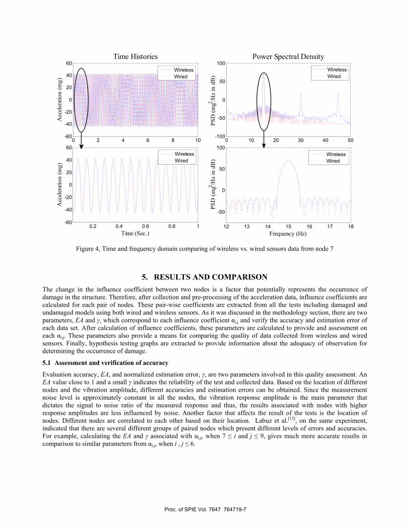
Figure 4, Time and frequency domain comparing of wireless vs. wired sensors data from node 7

5. RESULTS AND COMPARISON The change in the influence coefficient between two nodes is a factor that potentially represents the occurrence of damage in the structure. Therefore, after collection and pre-processing of the acceleration data, influence coefficients are calculated for each pair of nodes. These pair-wise coefficients are extracted from all the tests including damaged and undamaged models using both wired and wireless sensors. As it was discussed in the methodology section, there are two parameters, EA and γ, which correspond to each influence coefficient αi,j and verify the accuracy and estimation error of each data set. After calculation of influence coefficients, these parameters are calculated to provide and assessment on each αi,j. These parameters also provide a means for comparing the quality of data collected from wireless and wired sensors. Finally, hypothesis testing graphs are extracted to provide information about the adequacy of observation for determining the occurrence of damage.

5.1 Assessment and verification of accuracy

Evaluation accuracy, EA, and normalized estimation error, γ, are two parameters involved in this quality assessment. An EA value close to 1 and a small γ indicates the reliability of the test and collected data. Based on the location of different nodes and the vibration amplitude, different accuracies and estimation errors can be obtained. Since the measurement noise level is approximately constant in all the nodes, the vibration response amplitude is the main parameter that dictates the signal to noise ratio of the measured response and thus, the results associated with nodes with higher response amplitudes are less influenced by noise. Another factor that affects the result of the tests is the location of nodes. Different nodes are correlated to each other based on their location. Labuz et al.[13], on the same experiment, indicated that there are several different groups of paired nodes which present different levels of errors and accuracies. For example, calculating the EA and γ associated with αi,j, when 7 ≤ i and j ≤ 9, gives much more accurate results in comparison to similar parameters from αi,j, when i , j ≤ 6.

0 2 4 6 8 10-60

-40

-20

0

20

40

60A

ccel

erat

ion

(mg)

Time Histories

0 10 20 30 40 50-100

-50

0

50

100

PSD

(mg2 /H

z in

dB

)

Power Spectral Density

0.2 0.4 0.6 0.8 1-60

-40

-20

0

20

40

60

Time (Sec.)

Acc

eler

atio

n (m

g)

12 13 14 15 16 17 18

-50

0

50

100

Frequency (Hz)

PSD

(mg2 /H

z in

dB

)

WirelessWired

WirelessWired

WirelessWired

WirelessWired

Proc. of SPIE Vol. 7647 764719-7

Based on this understanding, it can be realized that nodes 7 through 9 have significantly higher amplitudes because their location is closer to the vibration source. On the contrary, nodes 1 through 6, which are along the column, exhibit smaller responses and lower signal to noise ratio because of the fixed boundary condition at each end of the column element. These characteristics of different node pairs of the structure are instrumental in choosing the influence coefficients for indicating the damage. Because the major focus for this study is validation of a WSN platform, the evaluation is centered on the EA and γ parameters obtained from data collected by the wired and wireless sensor networks. By inspection of the results associated with different node pairs, it can be seen that the wired data in compare with wireless data has slightly more accurate results. As two instances, Figure 5 shows the EA and γ parameters associated with two pairs of 5, 8 and 2, 5. Another parameter shown in these plots is the influence coefficients, αi,j, which is the damage indicator. The noticeable jump in αi,j from test number 15 (the last undamaged test) to 16 (the first damaged test), shows the potential damage in the structure.

(a) (b)

Figure 5, Comparison of Influence Coeff., α, Evaluation Accuracy, EA, and Estimation Error, γ. Wired Vs. Wireless: (a) influence coefficient α58, (b) influence coefficient α25

Figure 5 shows that both systems are capable of presenting changes in αi,j. These results show that the WSN results are accurate enough for this damage detection technique. It is also noticeable that the result from α58, with higher response amplitude, is more accurate than α25, with small response amplitude. As discussed before, this is due to the signal to noise ratio of the collected data.

5.2 Damage Detection

The damage indicator of this algorithm is the relative change in the influence coefficients during the transition of the intact system into the damaged system. Table 2 includes these relative changes in αi,j parameters, averaged over the tests before and after damage. Each number in the table corresponds to the changes in αi,j when i and j are row and column numbers of the table.

Influence coefficients of node pairs which are on opposite sides of the damage experience the largest changes after occurrence of the damage. This noticeable change, typically between 10 to 30%, can be observed for both wireless and wired sensors in Table 3. This trend in enables the algorithm to reflect the occurrence of the damage in the structure.

Since the damage has occurred in the beam element, it is expected that the αi,j, with i and j both from beam element, experience a relatively greater change in compare with αi,j, i and j both from undamaged column element. For example, the relative changes of the α parameters estimated between nodes 7, 8 and 9 should be greater than those parameters estimated from nodes 1, 2 and 3. Table 2 (a), shows this trend for the wired sensor results. By similar inspection on the WSN results, Table 2 (b), it can be seen that although a similar trend exists in the relative changes, the quantities of change are not as significant as that of the wired network. For instance, α7,9, which corresponds to two nodes on the beam element, has experienced 3.29% change whereas α3,1 and α4,6, which correspond to two parts of the undamaged column element, have experienced 2.72%. These changes are very comparable, and therefore, do not successfully identity the location of damage. However, it is important to note that such inconsistent parameters are not selected as significant damage indicators in the accuracy assessment process.

10

15

20

α 58

Node Pair 5 & 8: Wireless Vs. Wired

0 5 10 15 20 25 30

0.850.9

0.951

EA58

00.0010.0020.0030.0040.005

γ 58

Wireless Wired

Wireless Wired

Wired Wireless

Test Run Number

-1

-0.8

-0.6

α 25

Node Pair 2 & 5: Wireless Vs. Wired

0 5 10 15 20 25 30

0.850.9

0.951

EA25

00.0010.0020.0030.0040.005

γ 25

Wireless Wired

WirelessWiredWireless Wired

Test Run Number

Proc. of SPIE Vol. 7647 764719-8

Table 2-a, Changes in influence coefficients, αi,j. Wired Sensors Network

Table 2-b, Changes in influence coefficients, αi,j. Wireless Sensors Network

To further clarify the observed tendencies of relative changes in influence coefficients, Figure 6 graphically shows selected parametric changes for a direct comparison of the simulation, wired, and wireless results. The relative changes between two nodes i and j in this graph, are the average changes of αi,j and αj,i.

Figure 6, Comparison of relative change of influence coefficients between simulation, wired and wireless networks

Figure 6 shows that the data from the WSN is less apt at distinguishing between the damage and undamaged elements, as the changes for αi,j where 1 ≤ i, j≤ 6 versus that of αi,j where 7 ≤ i, j≤ 9are very similar. This difference in performance of

4

: location of damage

1

2

3

5

6

7 98

1

2

3

4

5

6

7 8 9

3.8%

Wireless NetworkWired Network

5.0%

3.6%

5.1%

20.7%

15.6%0.3%

8.2%

1.1%

4.8%

24.2%

31.6%

: location of accelerometer

3

6

5

4

2

1

7 98

0.0%

0.1%

0.2%

2.7%

39.2%

39.4%

Simulation

Node No.

1 2 3 4 5 6 7 8 9

1 0.04% 1.35% 9.27% 7.19% 6.96% 6.84% 17.33% 23.11% 2 0.55% 1.53% 9.67% 7.45% 6.61% 6.71% 17.18% 22.96% 3 2.18% 1.50% 10.85% 8.67% 7.72% 5.20% 15.53% 21.22% 4 12.07% 12.15% 14.10% 2.62% 3.20% 18.94% 30.62% 37.03% 5 8.84% 9.10% 10.97% 2.56% 0.71% 15.82% 27.19% 33.43% 6 6.64% 7.61% 9.60% 4.21% 1.56% 14.11% 25.31% 31.47% 7 6.41% 6.04% 4.51% 15.64% 13.49% 12.79% 9.82% 15.22% 8 14.77% 14.44% 13.05% 23.18% 21.22% 20.59% 8.94% 4.92% 9 18.76% 18.44% 17.12% 26.79% 24.92% 24.32% 13.20% 4.69%

Node No. 1 2 3 4 5 6 7 8 9 1 3.16% 0.47% 5.12% 4.99% 6.59% 17.29% 15.26% 21.37% 2 4.52% 0.32% 3.57% 3.66% 3.56% 19.20% 16.91% 23.02% 3 2.72% 0.72% 3.54% 3.81% 4.07% 18.85% 16.65% 22.80% 4 3.62% 6.96% 8.23% 0.24% 3.01% 27.16% 23.82% 30.34% 5 3.69% 6.40% 7.42% 0.19% 3.25% 26.10% 23.19% 29.64% 6 9.44% 12.74% 14.13% 3.98% 4.02% 33.04% 29.66% 36.33% 7 18.52% 16.13% 15.48% 19.38% 19.70% 20.88% 1.88% 3.29% 8 16.57% 14.31% 13.58% 18.21% 18.27% 19.71% 2.23% 5.24% 9 20.77% 18.61% 17.89% 22.29% 22.36% 23.75% 2.87% 5.00%

Proc. of SPIE Vol. 7647 764719-9

the wired and the wireless networks is likely due to the difference in noise characteristics and resolution of utilized accelerometers. However, it should be mentioned that the WSN system is still capable of detecting the existence of damage as well as the wired network system.

5.3 Hypothesis Test

A further verification of the two networks can be obtained via inspection of the hypothesis testing results. The hypothesis test graph indicates the required number of tests for concluding the occurrence of the damage to a 95% level of confidence. When the data crosses either of these two bounds, this corresponds to a positive hypothesis. The positive hypothesis, HA, as is explained in the Section 3.4 of this paper, indicates a 95%-confident detection of structural damage. Figure 7 shows the hypothesis test results for both the wired and wireless sensor networks on two pair-wise parameters. The evaluation accuracy and estimation error plots of these pairs of nodes are previously presented. The two parameters, accuracy and estimation error, associated with the nodes are the main parameters that dictate the point at which the damage is identified. More specifically, a higher EA and a lower γ will cause the confidence bounds to be crossed closer to the initial occurrence of damage. From a real-world application standpoint, this higher accuracy of data affords earlier recognition of damage based on a certain level of confidence.

(a) (b)

Figure 7, Comparison of Bayesian Test Results, Wired vs. Wireless: (a) Nodes 5 and 8 (α58), (b) Nodes 5 and 8 (α58)

In total 15 tests were run on the model after introducing the damage, and therefore, the run numbers in these plots range from 1 to 15. The first observation from these plots is that the wired sensor system is the first system to identify the occurrence of damage. This is reasonable based on the higher accuracy associated with wired system in all the results. The performance of wireless sensor for α58 is still acceptable since it does detect the damage, only a few tests after the wired system. In Figure 7 (b), it can be seen that the parameter α25, due to higher disturbance of noise in data, does not present qualified results for identifying the damage with 95% confidence level after 15 tests, whereas the wired sensor indicates damage after approximately 8 tests. However, it should be also mentioned that the α25 is not a strong damage indicator according to the accuracy assessment of the algorithm. There are many stronger indicators, such as α58 and α28, which relate nodes on opposite sides of the damage, and can, therefore, detect the damage much earlier.

6. CONCLUSION In this paper a WSN platform was experimentally validated using a damage detection algorithm with a densely clustered sensor network. The performance of the platform was evaluated based on several criteria of the damage detection algorithm. Generally, the evaluation showed an acceptable performance of WSN platform in which the system was fairly capable of detecting the damage. Accuracy and estimation error parameters were extracted for both wireless and wired networks. The WSN presented comparable error level to the wired network with piezoelectric sensors. It was shown that the WSN system reflected the occurrence of the damage as well as the wired sensor network. Bayesian hypothesis testing was performed on both wired and wireless results. The hypothesis test graphs indicated that the wired sensors typically detected the damage earlier than the wireless sensors. It was explained that in some cases, due to built-in accuracy assessments, WSN required more tests to confidently present the occurrence of the damage.

0 5 10 15-2.5

-2

-1.5

-1

-0.5

0

0.5

1

1.5

2

2.5

Run Number After Damage

Bay

esia

n Te

st

α58: Wireless Vs. Wired

Wired

Wireless

95% Confidence Bound

0 5 10 15-2.5

-2

-1.5

-1

-0.5

0

0.5

1

1.5

2

2.5

Run Number After Damage

Bay

esia

n Te

st

α25 : Wireless Vs. Wired

Wireless

95% Confidence BoundWired

Proc. of SPIE Vol. 7647 764719-10

7. ACKNOWLEDGMENTS The research described in this paper is supported by the National Science Foundation through Grant No. CMMI-0926898 by Sensors and Sensing Systems Program. The authors thank Dr. Shih-Chi Liu for his support and encouragement.

8. REFERENCES [1] Straser, E. G. and Kiremidjian, A. S., “A Modular, Wireless Damage Monitoring System for Structures,” Technical Report 128, John A. Blume Earthquake Engineering Center, Stanford University, Stanford, CA (1998).

[2] Lynch J. P., Loh K. J., “A summary review of wireless sensors and sensor networks for structural health monitoring,” The Shock and vibration digest ISSN 0583-1024, vol. 38, pp. 91-128 (2006).

[3] Farrar, C. R., Allen, D. W., Ball, S., Masquelier, M. P., and Park. G, “Coupling Sensing Hardware with Data Interrogation Software for Structural Health Monitoring,” Proc. 6th Int’l Symp. Dynamic Problems of Mechanics, Ouro Preto, Brazil (2005).

[4] Crossbow Technology, Inc, “MICAz Wireless Measurement System,” San Jose, CA (2007).

[5] Intel Corporation Research, Intel Mote2 Overview, Version 3.0, Santa Clara, CA (2005).

[6] Wang, Y., Lynch, J. P. and Law, K. H., “Validation of an integrated network system for real-time wireless monitoring of civil structures,” Proc. 5th Int’l Ws. Structural Health Monitoring, Stanford, CA, September 12-14 (2005).

[7] Pakzad, S.N., Fenves, G.L., Kim, S., and Culler, D.E, “Design and Implementation of Scalable Wireless Sensor Network for Structural Monitoring,” ASCE Journal of Infrastructure Engineering, 14(1):89-101 (2008).

[8] Pakzad, S.N., and Fenves, G.L., “Statistical analysis of vibration modes of a suspension bridge using spatially dense wireless sensor network,” ASCE Journal of Structural Engineering, 135(7):863-872 (2009).

[9] Whelan, M. J., Janoyan, K. D., “Design of a Robust, High-rate Wireless Sensor Network for Static and Dynamic Structural Monitoring,” Journal of Intelligent Material Systems and Structures, Vol. 20, No. 7, 849-863 (2009).

[10] Pakzad, S.N., “Development and deployment of large scale wireless sensor network on a long-span bridge,” Smart Structures and Systems, An International Journal, in press (2010).

[11] Rice, J. A. and Spencer Jr., B. F., “Structural health monitoring sensor development for the Imote2 platform,” Proc. SPIE Smart Structures/NDE (2008).

[12] Rice, J.A. and Spencer, B.F., “Flexible Smart Sensor Framework for Autonomous Full-scale Structural Health Monitoring,” NSEL Report Series, No. 18, University of Illinois at Urbana-Champaign (2009). (http://hdl.handle.net/2142/13635)

[13] Labuz, E. L., Chang, M., Pakzad, S., “Local Damage Detection in Beam-Column Connections Using a Dense Sensor Network,” to appear in Proc. of Structures Congress, Orlando, FL (2010).

[14] PCB Piezotronics, Inc, “Single axis capacitive accelerometer, series 3701,” NY, NY (2005) http://www.pcb.com/Linked_Documents/Vibration/VIB300E_1204.pdf

[15] Campbell Scientific, Inc, “CR9000X measurement and Control System,” Logan, UT, USA (1995).

[16] TinyOS, http://www.tinyos.net (2006).

[17] STMicroelectronics, “LIS3L02AS4 MEMS Inertial Sensor,” Geneva, Switzerland (2005).

[18] Quickfilter Technologies, Inc., “QF4A512 4-Channel Programmable Signal Conditioner,” Allen, TX (2007).

[19] ISHMP: http://shm.cs.uiuc.edu/software.html (2009).

[20] Chen, J., and Gupta, A.K. “Parametric change point analysis,” Birkhäuser, Boston (2000).

[21] Mazzonih, S., McKenna, F., Scott, M.H., and Fenves, G.L. “OpenSees Command Language Manual,” http://opensees.berkeley.edu/OpenSees/manuals/usermanual/index.html (2000)

Proc. of SPIE Vol. 7647 764719-11