Joris Falter

resultsship-ship interaction forces with captive model testValidation of a potential flow code for computation of

Academiejaar 2009-2010Faculteit IngenieurswetenschappenVoorzitter: prof. dr. ir. Julien De RouckVakgroep Civiele techniek

Master in de ingenieurswetenschappen: werktuigkunde-elektrotechniekMasterproef ingediend tot het behalen van de academische graad van

Begeleiders: Carlos Guedes Soares, Serge SutuloPromotor: prof. dr. ir. Marc Vantorre

i

Preface Ship-ship interaction is a topic which has been discussed various times in the past. The research

performed in previous years is very diverse, showing a lot of very different approaches to, on the

one side prediction methods, and on the other side experimental programs. The target of the

hereby presented thesis was to validate a prediction method designed by Serge Sutulo and Carlos

Guedes Soares at the Instituto Superior Tecnico in Lisbon, Portugal. The validation of this

interaction code was based on towing tank experiments executed by Marc Vantorre, Ellada

Verzhbitskaya (both Ghent University) and Erik Laforce (Flanders Hydraulics). This international

cooperation gave me the unique opportunity to spend one year to write this thesis in Lisbon,

supported by the knowledge and assistance from two universities.

The organisation necessary to do this thesis was not trivial, and therefore I want to give special

thanks to Serge Sutulo, Marc Vantorre and Carlos Guedes Soares to make my investigation, my

studies and my stay in Portugal possible. I also want to thank Xueqian Zhou for his important

contribution in modelling and interpolating the ship’s hullforms.

For me, the realization of this thesis trained me a lot in technical skills, organizational methods and

research which made it a great experience. I hope the results achieved for this thesis will be of a

great help in the further development of the interaction code.

ii

Admission of Use The author gives permission to make this master dissertation available for consultation and to copy

parts of this master dissertation for personal use.

In the case of any other use, the limitations of the copyright have to be respected, in particular with

regard to the obligation to state expressly the source when quoting results from this master

dissertation.

Joris Falter Lisbon 7

th July 2010

iii

Validation of a Potential Flow Code for Computation of Ship-Ship

Interaction Forces with Captive Model Test Results

by

Joris Falter

Dissertation presented to obtain the academic degree of

Master of Electromechanical Engineering

Promoter: Prof. Dr. Ir. Marc Vantorre

Supervisors: Prof. Dr. Serge Sutulo (IST, Lisbon),

Prof. Dr. Carlos Guedes Soares (IST, Lisbon)

Faculty of Engineering

Ghent University

Department of Civil Engineering

President: Prof Dr. Ir. Julien de Rouck

Academic year: 2009-2010

Summary An extensive set of comparisons has been executed in order to validate an online double body

potential flow interaction code based on the Hess & Smith panel method, created by Sutulo and

Guedes Soares at the Instituto Superior Técnico, Lisbon, Portugal. The experimental data was

obtained at Flanders Hydraulics (Antwerp, Belgium) by Vantorre, Verzhbitskaya and Laforce. The

situations investigated are two ship’s encountering or overtaking in shallow water. The two hulls

are parallel, the speed range encloses speeds between 0 and 12 knots. From the four models

used, three have lengths of approximately 290 metres and beams around 40 metres. The fourth

model has a length of 166 metres and a beam of 22 metres. Valuable results are obtained, for

either surge, sway and yaw for the different situations, in dimensionless shape. Besides that,

comparisons are made between calculations in steady and unsteady mode. The hull forms had to

be modelled and interpolated to a certain number of panels. The effect on the accuracy when

changing the number of panels on the ship hulls is also investigated, as well as the effect of

reducing the time step between calculations from one second to half a second. The written text

contains only the most striking results. The whole set of data is available on the enclosed CD.

Key-words: ship-ship interaction, potential-flow estimation, shallow water, double body panel method

iv

Validation of a Potential Flow Code for Computation of Ship-Ship Interaction Forces with Captive Model Test Results

Joris Falter

Supervisors: Prof. Dr. Serge Sutulo, Prof. Dr. Carlos Guedes Soares, Prof. Dr. Ir. Marc Vantorre

I. INTRODUCTION

Ship’s interacting when overtaking or encountering can

affect manoeuvring and course keeping of ships. These

effects are enhanced when the ships are manoeuvring in

shallow water. At the Technical University of Lisbon, a

relatively simple potential double body panel method has

been created. This code allows to do online computations

of interaction forces and moments without limitations on

the hull shapes, positions and motions of the bodies. The

modelling of the hulls is based on the classic Hess and

Smith panel method.

This method has been validated for overtaking and

encountering situations in shallow water, based on the

experimental program from Vantorre et al. (2002). More

then 60 situations were compared for the surge, sway and

yaw forces and moments. Besides this, also a study on the

difference in behaviour in steady and unsteady mode has

been executed, the influence of the number of panels has

been investigated, and the effect of changing the time step.

SYMBOLS

B beam

h water depth

bby clearance between ships

'N dimensionless yaw moment

T draught

'X dimensionless surge force

'Y dimensionless sway force

'ξ dimensionless distance between midships,

increasing with time

II. EXPERIMENTAL DATA

The tests were executed at the Flanders Hydraulics

shallow water towing tank (Antwerp, Belgium), equipped

for this occasion with an auxiliary carriage besides the main

planar motion carriage. The two models were free to heave

and pitch, and the own ship (on which the forces were

measured) was equipped with rudder and propeller running

at self-propulsion point. The different parameters varied

were: the models used, the water depth, the side clearance,

encounter or overtake, the speeds (0, 4, 8 and 12 knots) and

the drafts of the ships.

III. POTENTIAL FLOW INTERACTION CODE

The code only takes the potential flow interaction into

account, in this way neglecting viscous and free-surface

effects. The importance of each of these effects in the total

interaction force is not quite clear. The ship hulls are

doubled with respect to the water plane area, and because

the cases are in shallow water cases additional mirror

images with distance 2h were added. The neglecting of the

surface effects can be especially a problem at higher

speeds (for example, two ships encountering at 12 knots).

However, in the comparisons made, also for these

situations some good results are obtained.

IV. DIMENSIONLESS PARAMETERS

Results for forces and moments are given in the

following dimensionless shape, elaborated by professor

Sutulo:

( )

( )

2 2

1 1 2 2

2 2 2

1 1 2 2

2'

2'

i

i

i i

i

i

i i

FF

L T V V V V

MM

L T V VV V

ρ

ρ

=− +

=− +

(1)

V. SHIP MODELS

Four different ship models were used, scaled with a

factor 1:75. Their properties are displayed in table 1.

Table 1: Model Properties

Ship model C D E H

Ship type Bulk

carrier Container

ship Tanker Small tanker

Lpp m 3.984 3.864 3.824 2.21

B m 0.504 0.55 0.624 0.296

T m 0.18 0.18 0.207 0.125 0.178

CB - 0.843 0.588 0.816 0.796 0.83

The choice for the number of panels is based on the

findings in Sutulo S, Guedes Soares C. and Otzen J. (2010).

The numbers of panels used in the models is higher then in

this paper to obtain more realistic models, and to keep the

risk of errors due to bad modelling small.

The number of panels is shown in table 2.

Table 2: number of panels per model

Model C

Model D

Model E

Model H Own

Model H Target

886 896 932 554 544

The models are shown in figures 1 to 2.

x

y

x

Figure 1: Left: model C; right: model D

v

x

y

x

Figure 2: Left: model E; right: model H

VI. EXPERIMENTAL PARAMETERS

The cases covered are shallow water cases (1.2 < h/T <

1.5) and one very shallow water case (h/T < 1.2) with

respect to the ship with the largest draught.

The coordinate system is a common used, ship fixed

system, independent of the position of the target ship.

• X’: Nondimensional longitudinal force:

Positive if forward

• Y’: Nondimensional lateral force: Positive to

starboard side

• N’: Nondimensional yaw moment: Positive if

clockwise (from sky perspective)

Simulations were always done in this form:

• The own ship takes over the target ship: The target

ship is at port side of the own ship

• The target ship takes over the own ship: The own

ship is at starboard side of the target ship

• Encounter: Both ships are at port side with regard

to each other

VII. RESULTS

Comparisons for 62 situations with the standard

parameters have been done. Not all of them can be plotted

here. Only a few examples are shown. The own ship is the

ship on which the forces are measured. The dimensionless

stagger distance is increasing with time for all manoeuvres.

A. The own ship takes over the target ship

For these situations, the target ship had a speed of 8

knots, the own ship 12 knots. A good result is obtained for

the yaw moment when model H takes over model D, shown

in figure 3. The dashed line (with squares) is the

experimental result, the solid line is the computational

result.

ξ′s,n

, ξ′s,e

-1.5 -1 -0.5 0 0.5 1 1.5-0.03

-0.025

-0.02

-0.015

-0.01

-0.005

0

0.005

0.01

0.015

0.02

0.025

0.03

N′n

N′e

Figure 3: Yaw moment for model H taking over model D

The analysis of the data is based on visual results. Three

possible classifications for the results are:

• No agreement (X)

• Qualitative agreement: the same shape,

but not the same values (V)

• Quantitative agreement: the same shape and the

same values (VV)

This system is not very strict, and is more adopted here to

give an idea of the results obtained. The results for these

cases are given in table 4.

Table 4: results for the own ship taking over the target ship

surge sway yaw

No. of X 2 14 6

No. of V 11 0 5

No. of VV 1 0 3

Total 14 14 14

B.The target ship takes over the own ship

In most cases, the target ship had a speed of 12 knots, the

own ship 8 knots. Two cases with lower speed are also

present. The surge force for the case when model D gets

overtaken by model H is shown in figure 4.

ξ′s,n

, ξ′s,e

-2 -1.5 -1 -0.5 0 0.5 1 1.5 2-0.03

-0.025

-0.02

-0.015

-0.01

-0.005

0

0.005

0.01

0.015

0.02

X′n

X′e

Figure 4: Sway force for model D overtaken by model H

Using the same system of visual observation, following

results are obtained (table 5).

Table 5: Results for the own ship taken over by the target ship

Surge Sway yaw

No. of X 3 11 5

No. of V 11 4 8

No. of VV 2 1 3

Total 16 16 16

C. Encounter

There are 32 encounter cases. Most of them show good

results. In figure 5 model E (own ship) encounters model

D, both at 8 knots. The figure shown is the sway force.

The final results are shown in table 6.

vi

Table 6: Results for the encounter cases

surge sway yaw

No. of X 9 6 9

No. of V 13 20 12

No. of VV 10 6 11

Total 32 32 32

ξ′s,n

, ξ′s,e

Y′ n

,Y

′ e

-2 -1.5 -1 -0.5 0 0.5 1 1.5 2-0.3

-0.25

-0.2

-0.15

-0.1

-0.05

0

0.05

0.1

0.15

0.2

Y′n

Y′e

Figure 5: Sway force for model E encountering model D

D. Steady versus unsteady

All previous examples shown were calculated in the

unsteady mode, since the both ships have a relative speed

with respect to each other. However, when this relative

speed is small, calculations can also be done in unsteady

mode. The difference between both modes is the necessity

to calculate an unsteady term in the Bernouilli equation in

unsteady mode. Some calculations have been done to

compare both modes. In general results show that in

encounter cases, unsteady mode shows a lot less

discrepancies with the experimental results then the steady

mode. For the overtake cases, this is less clear, and

sometimes the steady mode results approximate the

experimental data better then the unsteady mode results.

E. Influence of the number of panels

To check the influence of the number of panels, the hull

forms were stripped down to a lower number. This was

mostly done in the midship section to maintain the

hullforms detailed enough in fore and aft.

Results are shown for the surge force for model E

(0 knots, own ship) overtaken by model D at 12 knots. The

number of panels was stripped down from 900 to 300 for

model E and from 900 to 400 for model D, with more or

less equal steps. As shown in figure 6, the effect is

marginal.

F. Influence of the time step

One comparison has been executed to compare the effect

of the simulation time step, which was reduced from 1

second to half a second. This could have allowed to

calculate the unsteady terms more accurate, but although

the two graphs are not completely the same, the difference

is not very significant.

VIII CONCLUSIONS

Validation of the code for interaction cases between two

ships in shallow water has been executed. Good results

have been obtained, but also larger discrepancies are

present. It is striking that the potential flow code calculates

in general very symmetric results, either around the origin

or around the vertical axis. The experimental results are not

always symmetric, meaning that discrepancies are almost

always present when this is not the case.

ξ′s

X'

-1.5 -1 -0.5 0 0.5 1 1.5-0.05

-0.04

-0.03

-0.02

-0.01

0

0.01

0.02

0.03

0.04

Exp

1E0D

1E1D2E2D

3E3D

4E4D

5E5D6E6D

Figure 6: Surge force for model E overtaken by model D,

7 situations with a different number of panels.

Possible reasons for the discrepancies are the freedom in

pitch and heave in the experiments, or the propeller

attached to the own ship. However, some results with a

speed of 0 knots for the own ship don’t confirm this theory.

An other possibility is the influence of the bottom. Results

have been compared for three equal cases with different

water depth, showing that especially for sway and yaw

results are better at larger depths.

A third option are the viscous effects which are not taken

into account. Small horizontal clearance can have an effect

on this (Sutulo, Guedes Soares and Otzen (2010)) but when

comparing results from situations were all parameters

except the clearance, it shows no trends which can either

confirm or deny this theory.

To calculate the influence of these effects, more

sophisticated interaction codes are necessary, however, the

speed obtained with this potential flow code is then lost.

REFERENCES

SUTULO, S.; GUEDES SOARES, C. (2008), Simulation of the Hydrodynamic Interaction Forces in Close-Proximity Manoeuvring, Proceedings of the 27

th Annual International Conference on

Offshore Mechanics and Arctic Engineering (OMAE 2008), Estoril, Portugal.

SUTULO, S.; GUEDES SOARES, C. (2009), Simulation of Close-Proximity Maneuvres Using an Online 3D Potential Flow Method, Proceedings of International Conference on Marine Simulation and Ship Manoeuvrability MARSIM 2009, Panama City, Panama

SUTULO, S.; GUEDES SOARES, C.; OTZEN J. (2010), validation of potential-flow estimation of interaction forces acting upon ship hulls in side-to-side motion at low Froude number, submitted for publication

VANTORRE, M.; LAFORCE, E; VERZHBITSKAYA, E (2002), Model test based formulations of ship-ship interaction forces, Ship Technology Research Vol. 49 – 2002

vii

Dutch Summary

Validatie van een potentiaal-stroom code voor de berekening van schip-schip interactiekrachten op basis van resultaten van

modelproeven Originele titel: Validation of a Potential Flow Code for Computation of Ship-Ship Interaction Forces with

Captive Model Test Results

Door: Joris Falter

Promotor: Prof. Dr. Ir. Marc Vantorre

Begeleiders: Prof. Dr. Carlos Guedes Soares, Prof. Dr. Serge Sutulo

1. Inleiding

De interactie tussen schepen die elkaar kruisen of inhalen kan het manoeuvreren en koers

houden van deze schepen danig beïnvloeden. Deze effecten worden nog eens versterkt wanneer

de schepen in ondiep water manoeuvreren. Sutulo en Guedes Soares (2008) hebben aan de

Technische Universiteit van Lissabon (Universidade Técnica de Lisboa – UTL) een relatief

simpele paneel methode ontwikkeld, waarbij gebruik gemaakt wordt van een verdubbeld lichaam.

Deze code laat toe om in real-time de interactiekrachten en -momenten te berekenen, zonder

beperking op de vorm van de lichamen, de posities en de bewegingen. De modellering van de

lichamen is gebaseerd op de klassieke Hess en Smith paneel methode.

Methodes die het gedrag van schepen voorspellen die kort bij elkaar varen zijn reeds eerder

ontworpen, voor zeer uiteenlopende situaties. Enerzijds zijn er de empirische methodes

gebaseerd op experimentele resultaten. Anderzijds zijn er de methodes die gebaseerd zijn op de

(gesimplificeerde) fysische processen. Een voorbeeld van die laatste zijn onder andere de

potentiaal-stroom theorie, of de slender-body theorie. Abkowitz e.a. (1976) hebben een dergelijke

slender-body theorie ontwikkeld voor twee lichamen in diep water. Ook Tuck and Newman (1984)

hebben de scheepsvorm benaderd als een rank profiel. Daarnaast verwaarloosden zij ook de

oppervlakteverschijnselen door te veronderstellen dat het Froude nummer nul is. Het

verwaarlozen van de oppervlakteverschijnselen is daarna nog opnieuw gedaan door Korsmeyer

e.a. (1993) die voor de eerste keer de Hess & Smith paneel methode gebruikten voor het

modelleren van de scheepsromp, een methode die voordien voornamelijk gebruikt werd in de

luchtvaart. Vantorre e.a. (2002) is een typisch voorbeeld van een empirische methode,

gebaseerd op een uitgebreid experimenteel programma over interactie tussen twee parallelle

schepen die mekaar kruisen en inhalen in ondiep water.

Met het opkomen van krachtigere computers werd geprobeerd meer effecten in rekening te

brengen. Pinkster (2004) gebruikte ook een potentiaal-stroom theorie, maar maakte wel een

aanpassing om de golfeffecten in rekening te brengen. Een van zijn resultaten was dat in ondiep

water de oppervlakteverschijnselen van groter belang zijn. Huang and Chen (2006) gaan een

hele stap verder en ontwikkelden een CFD (computational fluid dynamics – berekende vloeistof

viii

dynamica) code gebaseerd op de Navier-Stokes vergelijkingen. Deze methodes laten accurate

resultaten toe, en kunnen de verschillende verschijnselen die optreden in rekening brengen, maar

zijn tijdrovend en vereisen krachtige computers. Het verschil met dit type methodes en de

potentiaal-stroom methode van Sutulo and Guedes Soares (2008) is dat deze laatste een relatief

simpele code is, die toelaat snel tot resultaten te komen. Iets wat bijvoorbeeld vereist is voor een

typische simulator op de brug.

Deze potentiaal-stroom methode is gevalideerd geworden voor situaties in ondiep water voor

schepen die elkaar kruisen en inhalen. 62 verschillende situaties werden gesimuleerd en

vergeleken met de experimentele data uit Vantorre e.a. (2002). Het vergelijken van de

experimentele data met de resultaten van de interactiecode is gebeurd voor de schrik- en

verzetkrachten en voor het giermoment. Daarnaast is er een studie uitgevoerd naar het verschil

in gedrag wanneer de code uitgevoerd wordt in tijdsafhankelijke of niet tijdsafhankelijke modus,

wat een belangrijk verschil inhoudt in het berekenen van de Bernouilli-vergelijking. De schepen

waren gemodelleerd met panelen, waarbij een groter aantal panelen een nauwkeuriger resultaat

gaf, maar ook een toename van de rekentijd. Door het aantal panelen van de modellen te

variëren is geprobeerd een goed evenwicht te vinden tussen tijd en nauwkeurigheid. Ten slotte is

voor een specifieke situatie kort de invloed onderzocht van het aanpassen van het tijdsinterval

tussen twee opeenvolgende berekeningen. Ook hier was het mogelijk dat een korter interval

aanleiding gaf tot nauwkeuriger berekeningen, maar ook tot een toename van de rekentijd.

Symbolen

B Breedte

h Water diepte

bby Transverse afstand tussen schepen (van romp tot romp)

'N Dimensieloos giermoment

T Diepgang

'X Dimensieloze schrikkracht

'Y Dimensieloze verzetkracht

'ξ Dimensieloze afstand tussen het middenschip van beide schepen, toenemend met de tijd

2. Experimentele data

De experimenten werden uitgevoerd in de Flanders Hydraulics shallow water towing tank in

Antwerpen. Deze was, naast de hoofd-aandrijfkar, ook met een hulp-aandrijfkar uitgerust om het

tweede schip te kunnen bevestigen. Beide schepen waren vrij in de domp- en stampbeweging.

Het eigen schip (het schip bevestigd aan de hoofd-aandrijfkar en op hetwelk de krachten gemeten

werden) was daarnaast ook uitgerust met een roer en een propeller, die draaide in zijn zelf-

propulsiepunt. Het doelschip (bevestigd aan de hulp-aandrijfkar) was hiermee niet uitgerust. De

variable parameters van de ter beschikking gestelde data waren: het gebruikte model (vier

verschillende scheepsmodellen), de waterdiepte, de transverse afstand tussen de schepen,

ix

inhalen of kruisen, de snelheid (0, 4,8 of 12 knopen) en de diepgang van de schepen. De

schepen waren altijd parallel ten opzichte van elkaar.

De krachten waren opgeschaald volgens de wet van Froude. Voor de krachten werd dit:

Fship = λρ λL3 (2.1)

En voor de momenten:

Mship = λρ λL4 (2.2)

Waarin λL de schaalfactor naar lengte is en λρ een schaalfactor naar de waterdichtheid:

λL = 75 (2.3)

λρ = 1 (2.4)

3. Interactiecode

De interactiecode is gebaseerd op de potentiaal-stroom theorie, wat betekent dat de viskeuze en

de oppervlakte-effecten niet in rekening gebracht worden. In welke mate deze effecten bijdragen

tot de totale interactiekracht is echter niet duidelijk.

De scheepsromp wordt gespiegeld rond het wateroppervlak. Op deze manier vervalt de

grensvoorwaarde van het vrije oppervlak, omdat het wateroppervlak nu als symmetrievlak

fungeert. Deze grensvoorwaarde vereist echter lage Froude getallen, en zou bij hogere

snelheden (bijvoorbeeld een kruismanoeuvre tussen twee schepen die varen aan 12 knopen)

problematisch kunnen zijn. Er is echter vastgesteld dat ook voor deze situaties goede resultaten

verkregen worden. Daarnaast is er een grensvoorwaarde op de scheepsromp die niet toelaat dat

het water door de scheepsromp penetreert. In het geval dat de waterdiepte beperkt is door een

horizontale bodem, moet ook hier een grensvoorwaarde vastgelegd worden. Dit wordt gedaan

door de dubbele scheepsromp te spiegelen rond de horizontale bodems aan weerszijden van de

dubbele scheepsromp. Door dit een oneindig aantal keren te doen is nu ook het bodemvlak een

symmetrievlak, en kan er dus geen water door penetreren. In de praktijk is gebleken dat na vier

afspiegelingen aan beide zijden de reeks reeds mocht afgebroken worden (Sutulo and Guedes

Soares 2008), zie figuur 1.

Bij de initialisatie van het programma moeten een aantal belangrijke parameters ingegeven

worden. De algemene parameters zijn: het aantal lichamen, in tijdsafhankelijke modus of niet in

tijdsafhankelijke modus, de totale simulatietijd, het tijdsinterval tussen de berekeningen en de

snelheid van het water indien het stromend water is. Voor elk lichaam moet een

geometriebestand gemaakt worden, dat het lichaam in secties, en vervolgens in coördinaten per

x

sectie verdeelt. Voor elk lichaam moeten vervolgens de initiële positie, de initiële snelheid en de

versnelling gegeven worden, volgens twee lineaire coördinaten, en voor de gierbeweging.

Figuur 1: Een verdubbelde scheepsromp (de middelste) met twee afspiegelingen aan beide zijden

Het verschil tussen een tijdsafhankelijke en tijdsonafhankelijke berekening zit in de Bernouilli

vergelijking:

( )2 21

2r pp V V

t

φρ

∂ = − + − ∂

(3.1)

Indien een berekening in tijdsonafhankelijke modus wordt uitgevoerd moet de verstorings-

potentiaal φ niet berekend worden. Tijdsonafhankelijke berekeningen kunnen echter ook gebruikt

worden wanneer de relatieve snelheden van de lichamen ten opzichte van elkaar klein zijn, wat

resulteert in snellere berekeningen maar een lagere nauwkeurigheid.

Daarnaast zijn er een aantal hard gecodeerde parameters: de waterdiepte, de massadichtheid

van het water en het aantal afspiegelingen.

De code genereert na afloop van de berekeningen een “force” bestand, dat de krachten en

momenten op en de positie van alle lichamen weergeeft voor elke tijdsstap, en een “added mass”

bestand dat de toegevoegde massa bevat van de lichamen. Daarnaast was het ook mogelijk om

de code een driedimensionaal model van de lichamen te laten genereren om te plotten in Tecplot.

xi

4. Dimensieloze parameters

Om het schaaleffect te elimineren en om verschillende situaties met elkaar te kunnen vergelijken

zijn de experimentele en computerberekende resultaten dimensieloos gemaakt. De keuze van

geschikte formules is echter niet banaal, wanneer er meer dan één schip betrokken is. Zo is het

bijvoorbeeld belangrijk de snelheid van beide schepen te betrekken in de formules, daar beide

een rol spelen. Mogelijkheden werden gezocht in de beschikbare literatuur, maar hadden vaak

slechts betrekking op de snelheid van één van de schepen, of vermenigvuldigden beide

snelheden simpelweg, wat problemen oplevert als één van de snelheden nul is. Een

verdienstelijke poging is die van Brix (1993), waarin zowel van de snelheid, als van de lengte als

van de diepgang van beide schepen een gemiddelde werd genomen. De uiteindelijk gebruikte

formules werden voorgesteld door professor Sutulo:

( ) ( )2 2 2 2 2

1 1 2 2 1 1 2 2

2 2' , 'i i

i i

i i i i

F MF M

LT V VV V L T V VV Vρ ρ= =

− + − + 1,2i = (4.1)

Deze formules gebruiken de lengte en de diepgang van het eigen schip, maar de snelheden van

beide schepen. Ze geven een goed resultaat voor de snelheid in de situaties wanneer één van

beide schepen stilligt en wanneer beide even snel gaan. In het eerste geval wordt de snelheid van

het andere schip gekwadrateerd, in het andere geval de snelheid van beide schepen. Op die

manier zijn deze formules identiek aan de dimensieloze formules voor één schip.

De Froude nummers, gebaseerd op de lengte van het schip en de waterdiepte zijn dan als volgt:

2 2 2 2

1 1 2 2 1 1 2 2,i hi

i

V VV V V VV VFn Fn

gL gh

− + − += = 1,2i = (4.2)

De longitudinale en transverse afstanden tussen respectievelijk het midscheepse gedeelte van

beide schepen en de longitudinale symmetrievlakken van beide zijn de standaard formules:

( ) ( )1 2 1 2

1 2 1 2

2 2' , '

L L B B

ξ ξ η ηξ η

− −= =

+ + (4.3)

Alle resultaten die verderop besproken worden en die op de CD staan zijn gebaseerd op de

voorgaande formules. De gebruikte massadichtheid is die van zout water.

xii

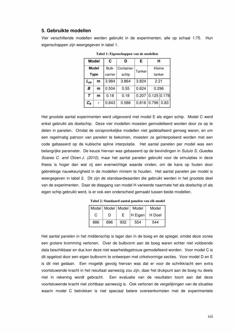
5. Gebruikte modellen

Vier verschillende modellen werden gebruikt in de experimenten, alle op schaal 1:75. Hun

eigenschappen zijn weergegeven in tabel 1.

Tabel 1: Eigenschappen van de modellen

Model C D E H

Model

Type

Bulk-

carrier

Container-

schip Tanker

Kleine

tanker

Lpp m 3.984 3.864 3.824 2.21

B m 0.504 0.55 0.624 0.296

T m 0.18 0.18 0.207 0.125 0.178

CB - 0.843 0.588 0.816 0.796 0.83

Het grootste aantal experimenten werd uitgevoerd met model E als eigen schip. Model C werd

enkel gebruikt als doelschip. Deze vier modellen moesten gemodelleerd worden door ze op te

delen in panelen. Omdat de oorspronkelijke modellen niet gedetailleerd genoeg waren, en om

een regelmatig patroon van panelen te bekomen, moesten ze geïnterpoleerd worden met een

code gebaseerd op de kubische spline interpolatie. Het aantal panelen per model was een

belangrijke parameter. De keuze hiervan was gebaseerd op de bevindingen in Sutulo S, Guedes

Soares C. and Otzen J. (2010), maar het aantal panelen gebruikt voor de simulaties in deze

thesis is hoger dan wat zij een evenwichtige waarde vinden, om de kans op fouten door

gebrekkige nauwkeurigheid in de modellen miniem te houden. Het aantal panelen per model is

weergegeven in tabel 2. Dit zijn de standaardwaarden die gebruikt werden in het grootste deel

van de experimenten. Daar de diepgang van model H varieerde naarmate het als doelschip of als

eigen schip gebruikt werd, is er ook een onderscheid gemaakt tussen beide modellen.

Tabel 2: Standaard aantal panelen van elk model

Model

C

Model

D

Model

E

Model

H Eigen

Model

H Doel

886 896 932 554 544

Het aantal panelen in het middenschip is lager dan in de boeg en de spiegel, omdat deze zones

een grotere kromming vertonen. Over de bulbvorm aan de boeg waren echter niet voldoende

data beschikbaar en dus kon deze niet waarheidsgetrouw gemodelleerd worden. Voor model C is

dit opgelost door een eigen bulbvorm te ontwerpen met cirkelvormige secties. Voor model D en E

is dit niet gedaan. Een mogelijk gevolg hiervan was dat er voor de schrikkracht een extra

voortstuwende kracht in het resultaat aanwezig zou zijn, daar het drukpunt aan de boeg nu deels

niet in rekening wordt gebracht. Een evaluatie van de resultaten toont aan dat deze

voortstuwende kracht niet zichtbaar aanwezig is. Ook vertonen de vergelijkingen van de situaties

waarin model C betrokken is niet speciaal betere overeenkomsten met de experimentele

xiii

resultaten dan de situaties waarin model D of model E betrokken is. Model H had geen bulbvorm

aan de boeg en had dus ook dit probleem niet.

De modellen met hun standaard aantal panelen zijn getoond in figuren 2 en 3.

x

y

x

Figuur 2: Links: Model C; Rechts: Model D

x

y

x

Figuur 3: Links: Model E; Rechts: Model H (eigen schip versie)

xiv

6. Parameters van de experimenten en de interactie code

6.1 Waterdieptes

De waterdieptes die gehanteerd werden in de experimenten zijn weergegeven in tabel 3. De

cijfers onder de modellen verwijzen naar de diepgang van de schepen. De cijfers in de tabel

verwijzen naar de waterdiepte.

Tabel 3: Standaarddiepgangen T van het eigen en het doelschip. De cijfers in de tabel verwijzen naar de

standaardwaterdiepte h (in het vet)

EIGEN T0

D E H

13.5 15.53 13.35 D

OE

L T

t

C

13.5 17.08 18.63 17.08 D

13.5 X

17.08

18.63 18.63

23.04

E

15.53 18.63 X 18.63

H

9.38 17.08 18.63 X

6.2 Assenstelsels

Het gebruikte assenstel is vastgemaakt aan het eigen schip. Het is onafhankelijk van de positie

van het doelschip.

• X’: Dimensieloze voorwaartse kracht: Positief indien voorwaarts

• Y’: Dimensieloze zijwaartse kracht: Positief naar de stuurboord zijde

• N’: Dimensieloos gier moment: Positief indien in klokwijzer-zin (uit vogel perspectief)

De simulaties werden gedaan op volgende manier:

• Het eigen schip haalt het doelschip in: Het doelschip bevindt zich aan de bakboordzijde

van het eigen schip

• Het doelschip haalt het eigen schip in: Het doelschip passeert aan de bakboordzijde van

het eigen schip

• Kruisen: Het kruisende schip bevindt zich aan de bakboordzijde van het eigen schip

De situaties zijn samengevat in figuur 4. De simulaties zijn op deze manier gedaan om de

assenstelsels van de experimentele resultaten en van de interactiecode te doen samenvallen.

6.3 Aantal afspiegelingen

Het aantal afspiegelingen is vastgelegd op vier voor alle simulaties die uitgevoerd werden voor

deze thesis.

6.4 Tijdstap

Het tijdsinterval tussen opeenvolgende berekeningen was vastgelegd op 1 seconde, zowel voor

de kruis- als voor de inhaalmanoeuvres. Deze keuze is gemaakt om een goed evenwicht te

vinden tussen rekentijd en nauwkeurigheid. De totale ingestelde simulatietijd van een

inhaalmanoeuvre was, afhankelijk van de snelheden van de schepen, ongeveer 500 seconden,

en van een kruismanoeuvre ongeveer 250 seconden.

xv

Figuur 5: Links: Het eigen schip (Own) haalt het doelschip (Target) in

Midden: Het doelschip (Target) haalt het eigen schip (Own) in

Rechts: Kruisen van het doelschip (Target) en het eigen schip (Own)

7. Resultaten van de vergelijkingen

62 Simulaties zijn uitgevoerd met de standaardparameters en in tijdsafhankelijke modus.

Vervolgens zijn er nog enkele vergelijkingen gemaakt tussen tijdsafhankelijke en

tijdsonafhankelijke modus, met een verschillend aantal panelen voor de modellen en met een

kleinere tijdstap. Deze konden niet allemaal grafisch weergegeven worden in de volledige tekst.

De meerderheid van de resultaten is dus enkel beschikbaar op de bijgevoegde CD.

De schepen waren altijd parallel ten opzichte van elkaar. De transverse afstanden ybb tussen

beide scheepsrompen waren meestal de helft van de breedte van het doel of van het eigen schip.

Enkele experimenten met kleinere en grotere afstanden werden ook uitgevoerd en zijn bijgevolg

ook gesimuleerd met de interactiecode. De gebruikte waterdieptes waren volgens de ITTC: één

“zeer ondiep water” situatie (h/T < 1.2) en de rest “ondiep water” situaties (1.2 < h/T < 1.5) met

betrekking tot het schip met de grootste diepgang.

De resultaten zijn niet op een wiskundige manier vergeleken. Om toch een evaluatie te kunnen

maken is een onderverdeling gemaakt in drie subcategorieën, gebaseerd op de visuele

resultaten:

• Geen overeenkomst (symbool: X)

• Kwalitatieve overeenkomst: de grafieken vertonen een gelijkaardig verloop qua vorm,

maar de waarden komen niet overeen (symbool: V)

• Kwantitatieve overeenkomst: de grafieken zijn gelijkaardig, zowel qua vorm als qua

waarden (symbool: VV)

xvi

Deze onderverdeling is subjectief en mag dus ook niet als een absoluut resultaat geïnterpreteerd

worden. Ze dient meer om zich een idee te vormen van de behaalde resultaten. Om deze reden

zijn er ook slechts drie onderverdelingen.

In alle grafieken die verderop worden weergegeven is de horizontale as de dimensieloze afstand

ξ’ en de verticale as de dimensieloze kracht of moment. Het subscript “n” staat voor de resultaten

van de interactiecode (volle lijn). Het subscript “e” voor de experimentele resultaten (streepjeslijn

met vierkantjes).

7.1 Het eigen schip haalt het doelschip in

In de uitgevoerde simulaties had het eigen schip altijd een snelheid van 12 knopen, en het

doelschip een snelheid van 8 knopen. In het totaal zijn er 14 verschillende situaties vergeleken.

Een goed resultaat is bekomen wanneer model H model D inhaalt (figuur 6), met standaard

waterdiepte en met een transverse afstand tussen beide schepen die de helft is van de breedte

van model D.

ξ′s,n

, ξ′s,e

-1.5 -1 -0.5 0 0.5 1 1.5-0.025

-0.02

-0.015

-0.01

-0.005

0

0.005

0.01

0.015

0.02

X′nX′e

ξ′s,n

, ξ′s,e

-1.5 -1 -0.5 0 0.5 1 1.5-0.08

-0.06

-0.04

-0.02

0

0.02

0.04

0.06

Y′nY′

e

ξ′s,n

, ξ′s,e

-1.5 -1 -0.5 0 0.5 1 1.5-0.03

-0.025

-0.02

-0.015

-0.01

-0.005

0

0.005

0.01

0.015

0.02

0.025

0.03

N′nN′

e

Figuur 6: Model H haalt model D in; Links: Schrikkracht; Midden: Verzetkracht; Rechts: Giermoment

De resultaten voor alle 14 situaties zijn weergegeven in tabel 4 volgens het eerder vermelde

systeem. Enkele trends zijn dat voor het verzetten de resultaten altijd slecht zijn. Dit is ook in

figuur 6 het geval. Voor schrikken en voor gieren zijn er enkele goede resultaten behaald.

Opmerkelijk is dat goede resultaten voornamelijk behaald worden indien het kleinere model H het

eigen schip is, zie hiervoor de resultaten op de CD.

Tabel 4: Evaluatie van de vergelijkingen voor het eigen schip dat het doelschip inhaalt

Schrikken Verzetten Gieren

Aantal X 2 14 6

Aantal V 11 0 5

Aantal VV 1 0 3

Totaal 14 14 14

7.2 Het doelschip haalt het eigen schip in

Voor deze situaties zijn er 16 simulaties vergeleken met de experimentele resultaten. In de

meerderheid van de situaties vaarde het eigen schip aan 8 knopen, en het doelschip aan 12

knopen. Slechts in twee gevallen had het eigen schip een lagere snelheid (respectievelijk 4 en 0

knopen). In figuur 7 is een situatie getoond met goede resultaten, namelijk model H dat model D

xvii

inhaalt, met standaardwaterdiepte en met een transverse afstand tussen beide die de helft van de

breedte van model D is.

ξ′s,n

, ξ′s,e

-2 -1.5 -1 -0.5 0 0.5 1 1.5 2-0.06

-0.04

-0.02

0

0.02

0.04 X′nX′e

ξ′s,n

, ξ′s,e

-2 -1.5 -1 -0.5 0 0.5 1 1.5 2-0.14

-0.12

-0.1

-0.08

-0.06

-0.04

-0.02

0

0.02

0.04

0.06

0.08

0.1

Y′nY′e

ξ′s,n

, ξ′s,e

-2 -1.5 -1 -0.5 0 0.5 1 1.5 2-0.06

-0.04

-0.02

0

0.02

0.04

N′nN′

e

Figuur 7: Model H wordt ingehaald door model D; Links: Schrikkracht; Midden: Verzetkracht; Rechts:

Giermoment

De resultaten voor deze situaties zijn samengevat in tabel 5. Betere resultaten zijn behaald dan

wanneer het eigen schip het doelschip inhaalt, zowel voor de schrikkracht, de verzetkracht als het

giermoment. Het aantal goede overeenkomsten in de verzetkracht blijft echter miniem. Opnieuw

is opvallend dat situaties waarin het model H betrokken is, merkelijk betere resultaten vertonen

(zie de bijgevoegde CD).

Tabel 5: Evaluatie van de vergelijkingen voor het doelschip dat het eigen schip inhaalt

Schrikken Verzetten Gieren

Aantal X 3 11 5

Aantal V 11 4 8

Aantal VV 2 1 3

Totaal 16 16 16

7.3 Kruisen

De 32 situaties waarin de twee schepen elkaar kruisen zijn zeer divers wat betreft snelheid. In

het merendeel van de situaties vaart één van beide of alle twee aan 12 of 8 knopen. In sommige

situaties is de snelheid van één van de schepen 4 of 0 knopen. Figuur 8 toont de resultaten voor

het kruisen van model E (eigen schip) met model D, beide aan 8 knopen, de situatie met de

grootste overeenkomsten van de kruismanoeuvres.

ξ′s,n

, ξ′s,e

-1.5 -1 -0.5 0 0.5 1 1.5-0.04

-0.02

0

0.02

0.04

X′n

X′e

ξ′s,n

, ξ′s,e

-1.5 -1 -0.5 0 0.5 1 1.5-0.3

-0.25

-0.2

-0.15

-0.1

-0.05

0

0.05

0.1

0.15

Y′n

Y′e

ξ′s,n

, ξ′s,e

-1.5 -1 -0.5 0 0.5 1 1.5-0.06

-0.04

-0.02

0

0.02

0.04

N′nN′

e

Figuur 8: Model E (eigen schip) kruist model D; Links: Schrikkracht; Midden: Verzetkracht; Rechts:

Giermoment

xviii

Eén van de problemen die optreden bij de kruismanoeuvres is dat de verschillen tussen de

experimentele resultaten en de resultaten van de interactiecode groot zijn wanneer de

interactiekrachten klein zijn. Dit is het geval wanneer de transverse afstand tussen beide

schepen groot is, of wanneer het doelschip een snelheid van 0 knopen heeft. Deze twee situaties

buiten beschouwing gelaten, kan geconcludeerd worden dat de kruissituaties veel betere

resultaten vertonen dan de inhaalsituaties, zoals valt af te lezen uit tabel 6. Een mogelijke reden

hiervoor is het Strouhal nummer, dat veel lager is voor een kruismanoeuvre (als de relatieve

snelheid tussen beide schepen als karakteristieke snelheid gekozen wordt) zodat de viskeuze

effecten minder belangrijk zijn (Sobey, 1982).

Tabel 6: Evaluatie van de vergelijkingen voor het kruisen van het eigen schip en het doelschip

Schrikken Verzetten Gieren

Aantal X 9 6 9

Aantal V 13 20 12

Aantal VV 10 6 11

Totaal 32 32 32

7.4 Tijdsafhankelijk contra tijdsonafhankelijk

Omdat de schepen in voorgaande situaties altijd een relatieve snelheid hebben ten opzichte van

elkaar, zijn alle simulaties uitgevoerd in tijdsafhankelijke modus. Wanneer de relatieve snelheid

tussen beide klein is, is het ook mogelijk om de simulaties in tijdsonafhankelijke modus te

berekenen. Enkele simulaties zijn uitgevoerd om beide te vergelijken:

• Model H (eigen schip) kruist model C, beide aan 8 knopen

• Model H (eigen schip) wordt ingehaald door model C, aan respectievelijk 8 en 12 knopen

• Model E (eigen schip) haalt model D in, aan respectievelijk 12 en 8 knopen

ξ′s,unst

, ξ′s,e

, ξ′s,st

N'

-1.5 -1 -0.5 0 0.5 1 1.5-0.06

-0.04

-0.02

0

0.02

0.04

0.06

SteadyExperimentalUnsteady

ξ′s,unst

, ξ′s,e

, ξ′s,st

N'

-1.5 -1 -0.5 0 0.5 1 1.5-0.06

-0.04

-0.02

0

0.02

0.04

0.06

0.08

SteadyExperimentalUnsteady

ξ′s,unst

, ξ′s,e

, ξ′s,st

N'

-1.5 -1 -0.5 0 0.5 1 1.5-0.06

-0.04

-0.02

0

0.02

0.04

0.06

SteadyExperimentalUnsteady

Figuur 9: Tijdsafhankelijk contra tijdsonafhankelijk; links: kruis manoeuvre; Midden: het eigen schip ingehaald

door het doelschip; Rechts: het eigen schip haalt het doelschip in

[Steady = tijdsonafhankelijk; Experimental = Experimenteel; Unsteady = tijdsafhankelijk]

Voor het kruismanoeuvre is de tijdsafhankelijke modus duidelijk beter dan de tijdsonafhankelijke.

Wanneer het eigen schip ingehaald wordt is dit ook nog altijd het geval, maar het verschil tussen

tijdsafhankelijk en tijdsonafhankelijk is duidelijk veel kleiner. Wanneer het eigen schip het

doelschip inhaalt benadert de tijdsonafhankelijke modus het experimentele resultaat beter,

hoewel ook hier de verschillen klein zijn.

xix

7.5 Invloed van het aantal panelen

De verschillende modellen werden gereduceerd in aantal panelen om de invloed hiervan op de

nauwkeurigheid te onderzoeken. Van elk model werden vier tot zes nieuwe versies gemaakt met

een verschillend aantal panelen. Het aantal panelen werd gereduceerd van ongeveer 900 tot 400

voor model E en D en van ongeveer 700 tot ongeveer 300 voor model H. Het grootste aantal

panelen werd verwijderd uit het midscheeps gedeelte. Het aantal panelen in de boeg en de

spiegel werd slechts weinig gereduceerd om een gedetailleerd model te behouden. Drie

verschillende situaties werden gesimuleerd met deze nieuwe modellen, situaties waarvoor met de

standaardmodellen reeds goede overeenkomsten waren behaald:

• Model E (eigen schip) aan 0 knopen, ingehaald door model D aan 12 knopen

• Model H (eigen schip) aan 8 knopen, ingehaald door model D aan 12 knopen

• Model E (eigen schip) aan 4 knopen, kruisend met model D aan 8 knopen

De schrikkrachten voor deze drie situaties worden getoond in figuur 10. Het verschil in

nauwkeurigheid is marginaal. De legendes vermelden nummers van 0 tot en met 6, waarbij 0

voor het model met het grootst aantal panelen staat, en 6 voor het kleinste aantal. Het model met

het standaard aantal panelen heeft nummer 1.

ξ′s

X'

-1.5 -1 -0.5 0 0.5 1 1.5-0.05

-0.04

-0.03

-0.02

-0.01

0

0.01

0.02

0.03

0.04

Exp1E0D

1E1D2E2D3E3D4E4D5E5D

6E6D

ξ′s

X'

-1.5 -1 -0.5 0 0.5 1 1.5-0.05

-0.04

-0.03

-0.02

-0.01

0

0.01

0.02

0.03

0.04

0.05

Exp1H0D1H1D3H3D4H4D5H6D

ξ′s

X'

-1.5 -1 -0.5 0 0.5 1 1.5-0.04

-0.03

-0.02

-0.01

0

0.01

0.02

0.03

0.04

Exp1E1D2E2D3E3D4E4D

Figuur 10: Effect van de reductie van het aantal panelen; links: model E ingehaald door model D; Midden:

Model H ingehaald door model D; Rechts: Model E kruist model D

7.6 Invloed van het tijdsinterval

Een situatie aan hoge snelheid en met korte transverse afstand tussen beide schepen kan grote

verschillen vertonen indien het tijdsinterval gereduceerd wordt. Daarom werd een

kruismanoeuvre tussen model D (eigen schip) en model H gekozen, beide aan 12 knopen en met

een transverse afstand van 11,1 meter. Het tijdsinterval werd gereduceerd van 1 seconde naar

een halve seconde. In figuur 11 is echter te zien dat er geen grote verschillen optreden.

8. Conclusies

Uit de verschillende resultaten zijn bepaalde besluiten te trekken. Een eerste is dat de resultaten

van de interactiecode in veel gevallen zeer symmetrisch zijn, ofwel rond de oorsprong, ofwel rond

de verticale as. Deze symmetrie is niet altijd terug te vinden in de experimentele resultaten, en

leidt zo tot discrepanties tussen beide. Een mogelijke oorzaak voor deze discrepanties zijn de

verschillen tussen de experimentele opstelling en de interactiecode. Zo waren de schepen vrij om

te dompen en te stampen in de experimenten, maar was het niet mogelijk dit te simuleren in de

xx

interactiecode. Daarnaast bezat het eigen schip een roer en een propeller in de experimenten,

die niet in rekening gebracht werden in de simulaties. Het effect van de propeller kan onderzocht

worden omdat twee van de situaties uit de beschikbare vergelijkingen niet lijden onder dit

probleem, namelijk wanneer het eigen schip een snelheid van 0 knopen heeft. Het vergelijken

van deze situaties met identieke situaties, maar waarin het eigen schip een snelheid van 4 of 8

knopen heeft, levert geen uitsluitsel op over het effect van het roer (Appendix I).

ξ′s

X'

-1.5 -1 -0.5 0 0.5 1 1.5-0.015

-0.01

-0.005

0

0.005

0.01

0.015

1 second

Experimental

1/2 Second

ξ′s

Y'

-1.5 -1 -0.5 0 0.5 1 1.5-0.15

-0.1

-0.05

0

0.05

0.11 secondExperimental

1/2 Second

ξ′s

N'

-1.5 -1 -0.5 0 0.5 1 1.5-0.02

-0.015

-0.01

-0.005

0

0.005

0.01

0.015

0.02

1 second

Experimental

1/2 Second

Figuur 11: Kruis manoeuvre tussen model D en model H, met gereduceerd tijdsinterval; Links: schrikkracht;

Midden: Verzetkracht; Rechts: Giermoment

Een ander belangrijk verschil zijn de oppervlakte-effecten. Er waren experimentele data

beschikbaar van drie kruismanoeuvres waarin behalve de waterdiepte alle andere parameters

identiek zijn. De vergelijkingen tonen aan dat, vooral voor de verzetkracht en het giermoment, de

verschillen tussen de experimentele resultaten en de resultaten van de interactiecode kleiner

worden wanneer de waterdiepte toeneemt (Appendix II).

Een derde mogelijkheid zit in het verwaarlozen van de viscositeit. Sutulo, Guedes Soares en

Otzen (2010) vermelden dat dit mogelijk gevolgen heeft bij kleine transverse afstand. Er zijn

verschillende situaties beschikbaar waarbij deze afstand systematisch gevarieerd wordt. Maar de

vergelijkingen tussen de experimentele data en de resultaten van de interactiecode kunnen geen

uitsluitsel geven over de invloed van de transverse afstand.

De resultaten van de interactiecode komen dus slechts ten dele overeen met de experimentele

data. Meer onderzoek zal moeten verricht worden om deze resultaten te bevestigen, om de code

in andere domeinen te valideren (bijvoorbeeld diep water) en om de trends die in deze thesis aan

het licht gekomen zijn verder te onderzoeken, en het domein waarin ze geldig zijn verder af te

bakenen.

Referenties

ABKOWITZ, M.A.; ASHE, G.M.; FORTSON, R.M. (1976), Interaction effects of ships operating in proximity in deep and shallow water, 11

th ONR symposium on naval hydrodynamics, London

BRIX, J. (1993), Manoeuvring Technical Manual, Seehafen Verlag, Hamburg HUANG, E.T.; CHEN, H-C (2006), Passing ship effects on moored vessels at piers, Proceedings prevention first 2006 symposium, Long Beach, California

ITTC: Final report and recommendations to 23rd

ITTC of the manoeuvring committee.

xxi

PINKSTER (2004), The influence of a free surface on passing ship effects, International Shipbuilding Progress, Vol. 51, No. 4 SOBEY, I. (1982), Oscillatory flows at intermediate Strouhal number in asymmetry channels, Journal of Fluid Mechanics 125 SUTULO, S.; GUEDES SOARES, C. (2008), Simulation of the Hydrodynamic Interaction Forces in Close-Proximity Manoeuvring, Proceedings of the 27

th Annual International Conference on

Offshore Mechanics and Arctic Engineering (OMAE 2008), Estoril, Portugal. SUTULO, S.; GUEDES SOARES, C. (2009), Simulation of Close-Proximity Maneuvres Using an Online 3D Potential Flow Method, Proceedings of International Conference on Marine Simulation and Ship Manoeuvrability MARSIM 2009, Panama City, Panama SUTULO, S.; GUEDES SOARES, C.; OTZEN J. (2010), validation of potential-flow estimation of interaction forces acting upon ship hulls in side-to-side motion at low Froude number, submitted for publication TUCK E.O.; NEWMAN J.N. (1974), Hydrodynamic Interactions between Ships, Proc. 10

th

Symposium on Naval Hydrodynamics, Cambridge, Mass., USA VANTORRE, M.; LAFORCE, E; VERZHBITSKAYA, E (2002), Model test based formulations of ship-ship interaction forces, Ship Technology Research Vol. 49 – 2002 VARYANI, K.S.; VANTORRE, M. (2005), Development of New Generic Equation for Interaction Effects on A Moored Container Ship Due to Passing Bulk Carrier, Vol. 147, IJMW Part A2, June 2005 11

xxii

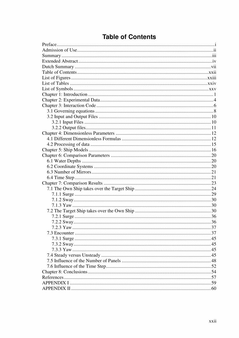
Table of Contents Preface ................................................................................................................................... i

Admission of Use ................................................................................................................. ii

Summary ............................................................................................................................. iii

Extended Abstract ............................................................................................................... iv

Dutch Summary ................................................................................................................. vii

Table of Contents ............................................................................................................. xxii

List of Figures ................................................................................................................. xxiii

List of Tables .................................................................................................................. xxiv

List of Symbols ................................................................................................................ xxv

Chapter 1: Introduction ........................................................................................................ 1

Chapter 2: Experimental Data .............................................................................................. 4

Chapter 3: Interaction Code ................................................................................................. 6

3.1 Governing equations .................................................................................................. 8

3.2 Input and Output Files ............................................................................................. 10

3.2.1 Input Files ......................................................................................................... 10

3.2.2 Output files ........................................................................................................ 11

Chapter 4: Dimensionless Parameters ............................................................................... 12

4.1 Different Dimensionless Formulas .......................................................................... 12

4.2 Processing of data .................................................................................................... 15

Chapter 5: Ship Models ..................................................................................................... 16

Chapter 6: Comparison Parameters ................................................................................... 20

6.1 Water Depths ........................................................................................................... 20

6.2 Coordinate Systems ................................................................................................. 20

6.3 Number of Mirrors ................................................................................................... 21

6.4 Time Step ................................................................................................................. 21

Chapter 7: Comparison Results ......................................................................................... 23

7.1 The Own Ship takes over the Target Ship ............................................................... 24

7.1.1 Surge ................................................................................................................. 29

7.1.2 Sway .................................................................................................................. 30

7.1.3 Yaw ................................................................................................................... 30

7.2 The Target Ship takes over the Own Ship ............................................................... 30

7.2.1 Surge ................................................................................................................. 36

7.2.2 Sway .................................................................................................................. 36

7.2.3 Yaw ................................................................................................................... 37

7.3 Encounter ................................................................................................................. 37

7.3.1 Surge ................................................................................................................. 45

7.3.2 Sway .................................................................................................................. 45

7.3.3 Yaw ................................................................................................................... 45

7.4 Steady versus Unsteady ........................................................................................... 45

7.5 Influence of the Number of Panels .......................................................................... 48

7.6 Influence of the Time Step ....................................................................................... 52

Chapter 8: Conclusions ...................................................................................................... 54

References .......................................................................................................................... 57

APPENDIX I ..................................................................................................................... 59

APPENDIX II .................................................................................................................... 60

xxiii

List of Figures Figure 1: Towing tank for manoeuvres in shallow water: General layout........................... 4

Figure 2: Main ship carriage ................................................................................................ 4

Figure 3: Auxiliary carriage ................................................................................................. 5

Figure 4: Underwater part of a single hull ........................................................................... 7

Figure 5: Underwater part mirrored ..................................................................................... 7

Figure 6: Underwater part, mirrored and with two mirrors on each side ............................ 7

Figure 7: Models’ Lineplans .............................................................................................. 17

Figure 8: Ship models: Model C and model D .................................................................. 18

Figure 9: Ship models: Model E and model H .................................................................. 18

Figure 10: Typical configuration: Model C (left) taking over model E (right), containing

1798 panels in total ............................................................................................................ 19

Figure 11: Coordinate system for own ship taking over target ship .................................. 22

Figure 12: Coordinate system for target ship taking over own ship .................................. 22

Figure 13: Coordinate system for encounter cases ............................................................ 22

Figure 14: Conventions and symbols (from: Vantorre et Al. (2002)) ............................... 23

Figure 15: Model H taking over model D .......................................................................... 26

Figure 16: Model H taking over model C .......................................................................... 26

Figure 17: Model D taking over model C .......................................................................... 27

Figure 18: Model D taking over model H .......................................................................... 27

Figure 19: Model D taking over model E with 10.31 metres of clearance ........................ 28

Figure 20: Model E taking over model C .......................................................................... 28

Figure 21: Model H taken over by model D ...................................................................... 32

Figure 22: Model D taken over by model H ...................................................................... 32

Figure 23: Model E taken over by model H ...................................................................... 33

Figure 24: Model E (4 knots) taken over by model D ....................................................... 33

Figure 25: Model D taken over by model E with 10.31 metres of clearance .................... 34

Figure 26: Model D taken over by model E with 41.25 metres of clearance .................... 34

Figure 27: Model E taken over by model C ....................................................................... 35

Figure 28: Model E (own ship) at 4 knots encountering model D at 8 knots .................... 40

Figure 29: Model H (own ship) at 8 knots encountering model C at 12 knots .................. 40

Figure 30: Model E (own ship) at 12 knots encountering model H at 12 knots ................ 41

Figure 31: Model E (own ship) at 8 knots encountering model D at 8 knots .................... 41

Figure 32: Model D (own ship) at 12 knots encountering model E at 0 knots .................. 42

Figure 33: Model E (own ship) at 12 knots encountering model C at 12 knots ................ 42

Figure 34: Model H (own ship) at 8 knots encountering model C at 8 knots .................... 43

Figure 35: Model H (own ship) at 8 knots encountering model C at 8 knots .................... 46

Figure 36: Model H taken over by model C ...................................................................... 47

Figure 37: Model E taking over model D .......................................................................... 47

Figure 38: Model D with different number of panels ........................................................ 49

Figure 39: Model E with different number of panels ........................................................ 50

Figure 40: Model H with different number of panels ........................................................ 50

Figure 41: Model E (own ship) at 0 knots overtaken by model D at 12 knots .................. 51

Figure 42: Model H (own ship) at 8 knots overtaken by model D at 12 knots .................. 51

Figure 43: Model E (own ship) at 4 knots encountering model D at 8 knots .................... 52

Figure 44: Model D (own ship) encountering model H, both at 12 knots ......................... 53

xxiv

List of Tables Table 1: Denominators to make the forces dimensionless ................................................. 15

Table 2: Model Properties .................................................................................................. 16

Table 3: Real size properties .............................................................................................. 16

Table 4: Number of panels for each ship ........................................................................... 17

Table 5: Standard water depths and standard drafts. ......................................................... 20

Table 6: Performed Comparisons for the own ship taking over the target ship ................ 25

Table 7: Performed comparisons for the own ship taking over target ship, dimensionless

............................................................................................................................................ 25

Table 8: Comparisons for the own ship taking over the target ship: evaluation ................ 29

Table 9: Performed comparisons for the target ship taking over the own ship ................. 31

Table 10: Performed comparisons for the target ship taking over the own ship,

dimensionless ..................................................................................................................... 31

Table 11: Comparisons for the target ship taking over the own ship: evaluation .............. 36

Table 12: Performed comparisons for encounter ............................................................... 38

Table 13: Performed comparisons for encounter: dimensionless ...................................... 39

Table 14: Comparisons for encounter: evaluation ............................................................. 44

Table 15: Model E (own ship) at 0 knots taken over by model D at 12 knots .................. 48

Table 16: Model H (own ship) at 8 knots taken over by model D at 12 knots .................. 48

Table 17: Model E (own ship) at 4 knots encountering model D at 8 knots ..................... 48

xxv

List of Symbols B1, B2 Own/target ship beam

Fship Force acting on the ship

Fn Froude number

h Water depth

L1, L2 Own/target ship length between perpendiculars

Lpp Length between perpendiculars

Mship Moment acting on the ship

N Yaw moment

Nn’, Ne’ Dimensionless computational yaw moment, dimenionless experimental yaw

moment

T1, T2 Own/target ship draft

V1, V2 Own/target ship speed

X Surge force

Xn’, Xe’ Dimensionless computational surge force, dimenionless experimental surge

force

Y Sway force

Yn’, Ye’ Dimensionless computational sway force, dimenionless experimental sway

force

η1, η2 Own/target ship transverse distance in an earth fixed reference system

η’ Dimensionless transverse distance between ships

λL Length scaling factor

λρ Water density scaling factor

ξ 1, ξ 2 Own/target ship forward distance in an earth fixed reference system

ξ ’ Dimensionless stagger distance between both ships

ρ Water density

1

Chapter 1: Introduction In the voyages made in their lifetime, ships encounter more then once restricted waters in which to

navigate. These restricted waters can affect the manoeuvring and course keeping of the ship.

Increasing ship sizes but restricted waters which maintain equally sized make this problem even

more crucial.

The interaction effects with the ship are caused by several factors. Bottom and bank effects, fixed

obstacles like piers and jetties or interaction with passing or encountering ships. Research has

been done on these effects and numerous papers are written on this topic. Unfortunately the

methods of investigation are sometimes very different in relation to each other. Besides that, there

are innumerable different situations in which interaction can take place, like for instance: overtaking

and encounter with parallel ship’s or not, the ships’ speeds, the water depth, the clearance, the

bank shapes, blockage factor … Most papers cover only one or two specific settings.

In the different publications available are two separate groups: experimental methods versus

theoretical based methods. The first allows to gather accurate data on ship behaviour and forces.

From this, numerical models can be extracted, whether or not with a strong theoretical background.

The weakness of experimental methods is their field of application. Since there are innumerable

different situations, either innumerable different experiments should be done to cover the whole

scene, or extrapolations are necessary. Besides that, experimental research is in most cases time-

consuming.

The other research technique are theoretical based computational methods. They consist of a

theoretical basis from which, with simplifications and numerical calculations, a mathemathical

solution is extracted. Simplifications of the theoretical model are necessary because, depending on

the approximation method, a lot of computational power can be required. Some examples of these

methods are the potential flow theory, slender-body theory and computational fluid dynamics (CFD)

methods. Mostly they allow to calculate solutions for problems which are more diverse, having

thus a larger field of appliance then experimental methods. The computational methods though

have to be validated according to experimental results to determine their accuracy.

A lot of methods have already been developed previously and attempts have been made to

validate them. Also the idea of using potential flow theory has been discussed before.

Abkowitz et al. (1976) created a slender-body theory for two bodies in infinite fluid at moderate

speed . Lagally’s theorem is used to calculate forces and moments, including also the unsteady

terms. The results are compared with experiments from different sources but show large

discrepancies. King (1977) did comparisons for ship interaction in shallow water based on a

2

double hull slender-body theory for unsteady ship interactions. The comparisons are however, only

limited to moored vessel experiments obtained by Remery (1975) and Yeung (1977).

Tuck and Newman (1984) devised two interaction theories, based on slender hulls and with zero

Froude number which were afterwards compared to experimental results. They emphasize the use

of potential flow theory, being likely to be of more importance then the free surface effects.

Kolkman (1987) gives basic considerations on flow patterns for ships manoeuvring in restricted

waters and currents. A short part discusses the influences of self-propelled and towed ships, and

the difference in waves they produce. Korsmeyer, Lee and Newman (1993) made an interaction

code neglecting wave effects by using a rigid, free water surface and the use of 3D models, which

are based on the Hess & Smith panel method. The results are compared with experiments for the

overtaking manoeuvre of two ships in a rectangular canal and one with sloped sides. The channels

boundary’s are represented by plane quadrilateral or triangular panels. Kyulevcheliev et al. (2003)

did a set of model experiments about the hydrodynamic impact of a moving ship on a stationary

ship in restricted water, for inland ships in a canal. Attention is also given to the influence of wave

effects. They come to the conclusion that their results show differences with other experimental

results. Possible reasons are the use of a barge with a box-shaped stern, and intensive wave

generation at higher speed and smaller canal dimensions. Their findings are confirmed by using a

no free-surface CFD simulation. Pinkster (2004) created a double hull potential flow method and a

potential flow method taking the wave effects into account. After, both were compared to

experimental results. The comparisons are specifically for the moored ship cases. Noticed is that

in open water surface effects become negligible for moored ships (for example jetty’s not to close

to the shore). Huang and Chen (2006) presented a practical case of the calculation of forces on a

moored vessel. Computations were made with a Chimera, Reynolds-averaged Navier-Stokes

based computational fluid dynamics model. Their model is able to calculate surface effects,

viscous effects and takes seafloor and bank geometry into account. Results are compared with

towing-tank and field tests. This type of computations is very accurate and complete in their

calculations but requires more calculating power.

The previous examples show that a lot of prediction models have already been made, some more

successful then others. The code used for this thesis has as an important advantage with regard to

the others that it is a relatively simple code, allowing online computations on commonly used

hardware.

The experimental data used in this thesis was presented in Vantorre et al (2002). They did a

comprehensive ship-ship interaction test program, involving four models, with different lateral

clearances, draught’s, speeds and under-keel clearances. Previously, Varyani and Vantorre

(2005) used this data to compare with generic equations for ship-ship interaction forces. These

generic equations are based on inviscid and incompressible fluid without free surface effects. The

comparisons were only done for the forces induced by a passing ship on a moored ship, using

three different water depths.

3

The interaction code used in thesis, was presented in Sutulo and Guedes Soares (2008). The

algorithm calculates the potential flow forces and is based on the Hess and Smith panel method,

using a double hull method. This allows to predict interaction loads with any number of objects in

real-time on a typical modern computer. In the same paper, a first validation was done by

comparing a tug – cargo vessel simulation to an empiric method. In Sutulo and Guedes Soares

(2009) the interaction code was used to simulate trajectories and time histories for two interacting

ships in uncontrolled and controlled motion. The two ships were identical with a length of 175m,

breadth 25.4m and draft 9.5m. Sutulo, Guedes Soares and Otzen (2010) did a validating for the

case of a tug operating near a larger vessel. The ship’s centerplanes were parallel and the

experiments were run in the steady regime. Both ships were un-propelled and fixed in all degrees

of freedom. One of their conclusions is that the worst agreement happens for the surge force and

for the sway force at very small horizontal clearance.

In present thesis, the validating of Sutulo’s and Guedes Soares’ interaction code has been

continued, comparing the interaction experiments from Vantorre with the results obtained by the

code. In the next two chapters, detailed explanations are given about the experimental program

and the interaction code. The following chapter is about the possibilities in making the data

dimensionless. The properties of the four models and the interpolation process are explained in

chapter 5. Before coming to the numerical results, some information is given on the coordinate

systems and the different parameters that are used. In the end, conclusions are drawn on the

comparison results.

4

Chapter 2: Experimental Data The experimental data used for the comparison was recorded by M. Vantorre, E Verzhbitskaya and

E. Laforce. The results from their investigation were published in “Model Test Based Formulations

of Ship-Ship Interaction Forces” in 2002.

The experiments were executed at the Flanders Hydraulics shallow water towing tank in Antwerp,

Belgium. This tank has a useful length of 67 metres (total length 88 metres), a width of 7.0 metres

and a maximum water depth of 0.5 meters (see figure 1). To make the interaction experiments

possible, an auxiliary carriage was installed besides the main planar motion carriage (see figures 2

and 3).

Figure 1: Towing tank for manoeuvres in shallow water: General layout (from Vantorre et Al. (2002))

Figure 2: Main ship carriage

The tests were executed with two models, the own ship and the target ship, being towed at variable

speeds. The own ship, equipped with rudder and a propeller running at self-propulsion point, was

free to heave and pitch, and was the only one on which measurements were made. The target

ship, without propeller and rudder, was also free to heave and pitch, but was not measured on.

The ships were always parallel to each other and all experiments were executed in shallow water.

Four ship models were used to perform the tests, one bulk carrier (model C), one container ship

(model D), one tanker (model E) and one small tanker (model H). The real size lengths varying

from 166 meters for the small tanker to 299 meters for the bulk carrier and the real size widths

varying from 22.2 meters for the small tanker to 46.8 meters for the tanker.

5

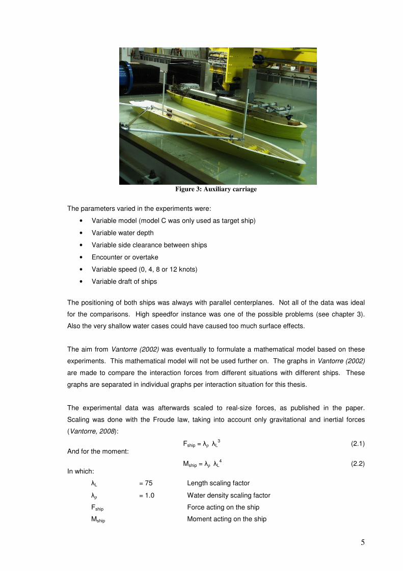
Figure 3: Auxiliary carriage

The parameters varied in the experiments were:

• Variable model (model C was only used as target ship)

• Variable water depth

• Variable side clearance between ships

• Encounter or overtake

• Variable speed (0, 4, 8 or 12 knots)

• Variable draft of ships

The positioning of both ships was always with parallel centerplanes. Not all of the data was ideal

for the comparisons. High speedfor instance was one of the possible problems (see chapter 3).

Also the very shallow water cases could have caused too much surface effects.

The aim from Vantorre (2002) was eventually to formulate a mathematical model based on these

experiments. This mathematical model will not be used further on. The graphs in Vantorre (2002)

are made to compare the interaction forces from different situations with different ships. These

graphs are separated in individual graphs per interaction situation for this thesis.

The experimental data was afterwards scaled to real-size forces, as published in the paper.

Scaling was done with the Froude law, taking into account only gravitational and inertial forces

(Vantorre, 2008):

Fship = λρ λL3 (2.1)

And for the moment:

Mship = λρ λL4 (2.2)

In which:

λL = 75 Length scaling factor

λρ = 1.0 Water density scaling factor

Fship Force acting on the ship

Mship Moment acting on the ship

6

Chapter 3: Interaction Code

The interaction code which was to be validated is a potential flow, double body method, based on

the Hess and Smith panel method. It was published in 2008 in “Simulation of the hydrodynamic

interaction forces in close-proximity manoeuvring” by Sutulo S. and Guedes Soares C. Later, in

2009, followed by “Simulation of close-proximity maneuvers using an online 3D potential flow

method” and later on, in a paper submitted for publication, validated in a tanker-tug situation in

“Validation of potential-flow estimation of interaction forces acting upon ship hulls in side-to-side

motion at low Froude number”. The code allows online calculation of interaction forces for multiple

moving and fixed objects for different positions and speeds. The computing power of an average

PC these days allows this process to be done in real-time. The present chapter will give a

summary of the interaction code’s properties, which are explained fully in these three papers.

Hydrodynamic interaction can be subdivided into five parts (Sutulo, S., Guedes Soares C., Otzen

J., 2010):

1. Near-field potential interaction

2. Interaction related to the free-surface effects or wavemaking interaction

3. Boundary layer and viscous wake interaction

4. Interaction caused by longitudinal trailing vortices

5. Action of propeller slipstreams and of the thrusters’ jets

It’s not clear what the contributions of the different components are in the total interaction force.

The interaction code created by Sutulo and Guedes Soares is based on the potential flow

interaction (and thus takes only the first point into account). This choice is made since certain

experience and data accumulated indicate that near-field double body potential interaction can be

the most important component in these cases (Sutulo, S., Guedes Soares C., Otzen J., 2010).

Potential flow interaction includes assuming perfect, inviscid and thus irrotational fluid.

In the experiments executed by Vantorre, however the first four components from the list above are

always present. The last is only created by the own ship (since it was equipped with a propeller)

but has an influence as well on the target ship. However, in the experiments the target ship was

never directly in the propeller’s slipstream, clearances between both ships were in most

experiments half of either the beam of the target or the own ship, only in few cases this clearance

is smaller. Cases in which this influence is not present is when the own ship ‘moves’ at zero

speed. The results for these cases don’t show any peculiar improvement in comparison to cases

where the own ship has a non zero speed.

Ship models are simulated with the classic Hess and Smith panel method (Hess, J.L; Smith, 1967).

This means that the body surface is represented as a set of flat quadrilateral elements with

constant source density on each of them. The ship hulls are doubled with respect to the free

7

surface (figures 4 and 5), in this way requiring only boundary conditions at infinity and on the ship

hull. The waterplane surface acts as a symmetry plane which makes waves impossible. This

requires low Froude numbers to be able to neglect the free surface effects. However, as will be

shown further on, in some encounter cases results are still good for two ships going both a speed

of 12 knots.

Figure 4: Underwater part of a single hull

Figure 5: Underwater part mirrored

Figure 6: Underwater part, mirrored and with two mirrors on each side (in the simulations four

mirrors on each side were used)

Because the experiments were conducted in shallow water (horizontal flat bottom), also mirror

images are necessary (figure 6). They create a series of double hulls with the distance 2h (in which

h is the water depth) between the waterplanes. Theoretically this should be an infinite series of

double hulls, in this way using the same principle as the water surface, namely that the bottom acts

as a symmetry plane through which penetration of the fluid is impossible. In practice, the number

of mirror images used in the comparisons performed was limited to four on each side, allowing

8

acceptable accuracy with acceptable calculating times. This choice is based on Sutulo, S., Guedes

Soares C., Otzen J., (2010) which states that four mirrors will be sufficient in most cases.

The Bernoulli equation used in the potential flow method is different for steady and unsteady cases.

This makes that in the input file for the program a distinction must be made between the two

different modes. Since both ships in the experiments performed always had different speeds, or

went in a different direction, all comparisons are done in unsteady mode. However, in chapter 7 a

section is dedicated to the comparison between unsteady and steady results.

The numerical algorithm used was coded as a Fortran 90 module. The computer program on which

the simulations were run was Visual Fortran 6.0 Developer Studio.

3.1 Governing equations A perfect fluid with irrotational flow can be described with the potential function Φ :

cur curV Vξ ηξ η φΦ = + + (3.1)

This function consists of two terms related to the current, and a perturbation potential ( , , , )tφ ξ η ζ

in which ξ is the advance, η the transfer, ζ the heave motion and t the time( which only matters

in unsteady problems). This perturbation potential satisfies the governing Laplace equation:

0φ∆ = (3.2)

The boundary conditions are a non-penetration boundary condition on each body:

rV n

n

φ∂=

∂i (3.3)

And a condition on the free surface (due to the low-Froude-number assumption) and on the flat

horizontal bottom:

0φ

ζ

∂=

∂ (3.4)

In the non-penetration boundary condition, the n is the outer unity normal to each body. Vr is the

relative local velocity, obtained by subtracting the current velocity from the absolute local velocity of

a point on the body surface. The code can also work for infinite depth, in this case the flat bottom

condition is not present and the perturbation potential must vanish at infinity.

9

The solution of previous problem is done by distributing of a single layer of sources with density σ

on the entire wetted surface. This leads to a Fredholm integral equation of the second kind,

containing a Green-function, which is different depending on the presence of a finite depth or not.

In the cases presented in this thesis, the depth is always finite, and the formulation has thus the

following form:

1 1

( , , , ', ', ')i i i

G x y z x y zr r

∞

=−∞

= +

∑ (3.5)

In which the right hand side term is an infinite series of double hull images, and

( ') ( ') ( ')r x x y y z z= − + − + − and ( ') ( ') ( ')r x x y y z z= − + − + + . The influence of the

farther images however is very small and therefore this series is, like mentioned before, limited to

i = 4.

Solving the Fredholm equation allows expressing the induction velocity and the potential

distributions through the already known single-layer density:

( ) ( ) ( , )d ( )

( ) ( ) ( , )d ( )

I M

S

S

V M P G M P S P

M P G M P S P

σ

φ σ

= ∇

=

∫

∫ (3.6)

The pressure distribution on the panels is obtained by using the unsteady Bernouilli equation

(Lamb, 1968):

( )2 21

2r pp V V

t

φρ

∂ = − + − ∂

(3.7)

In which ρ is the fluid density and

p I rV V V= − (3.8)

VI is the induction velocity expressed through the single-layer density σ(M) which can be obtained

by solving the Fredholm equation mentioned before. The Bernouilli equation shows what is

different between an unsteady and a steady calculation: in the unsteady case the perturbation

potential needs to be evaluated in every time step.

This can then be integrated to obtain the potential force Fpi and moment Mpi acting on the I th body:

i

pi

S

F pndS= −∫ (3.9)

10

i

pi

S

M pr ndS= − ×∫ (3.10)

In which p is the pressure, n is the outer unity normal to each body and S is the panel surface.

The forces and moments obtained by evaluation of previous formulas contain the added masses,

which have to be subtracted to get the net forces and moments on the objects. Sutulo and Guedes

Soares do this based on the equations from Thomson, Tait and Kirchoff (Lamb, 1968). The kinetic

energy from the fluid in the presence of a moving rigid body is represented as:

6

, 1

1

2jk j k

j k

T µ ω ω=

= ∑ (3.11)

In whichj

ω are the three linear velocities (i = 1, 2, 3) and the three rotational velocities (I = 4, 5, 6)

and jk

µ are the added mass coefficients for the i th body as:

d

i

jk j k

S

m Sµ ρ φ= − ∫ (3.12)

Where m1, m2, m3 are the projections of the normal n onto the body axes x, y and z. m4, m5, m6 are

similar projections of r x n. The potentials j

φ are obtained as a solution to the Fredholm equation.

The formulation of the proper hydrodynamic interaction forces is then eventually:

11 22

22 26 11

26 66 11 22 26( )

e

e

e

X u vr

Y v r ur

N v r uv ur

µ µ

µ µ µ

µ µ µ µ µ

= − +

= − − −

= − − + − −

�

� �

� �

(3.13)

The pure interaction forces are then:

; ;I p e I p e I p e

X X X Y Y Y N N N= − = − = − (3.14)

3.2 Input and Output Files

3.2.1 Input Files The input files contain a data file and the files which contain the model geometry (one file per

object). This geometry file divides the body in sections and then the sections in offsets.

11

The input files requests an input for:

• Number of bodies involved

• Steady or unsteady

• Total simulation time (seconds)

• Time step (seconds)

• Current velocity (two coordinates in an earth-fixed coordinate system)

Besides that, for every object, three degrees of freedom are present, as an initial value, a speed

and an acceleration parameter:

• Initial advance position (metres)

• Initial transfer position (metres)

• Initial heading (degrees)

• Initial advance velocity (m/s)

• Initial transfer velocity (m/s)

• Initial rate of yaw (dg/s)

• Advance acceleration

• Transfer acceleration

• Yaw acceleration

Other parameters are hard-coded, like the water depth, the water mass density and the number of

mirrors.

From these parameters, some are only used once at the initialization of the program. The

subroutine “Hydro_Interaction_Response” requires at every time step the number of bodies, the

time, three position coordinates and three quasi-velocities. The calculation mode (steady or

unsteady) is set at the initialization of the program, as well as the current speed by subtracting it

from the initial velocities. The present time is calculated by multiplying the time step with the

number of calculation steps already executed. With the time known, it is possible to calculate the

present speed by summing the initial speed with the multiplication of the acceleration and the

present time. Integrating this equation will give the present position, these parameters for speed

and position are then used in the Hydro_interaction_Response subroutine. Every initial parameter

describing position, speed and acceleration is thus used at every time step.

3.2.2 Output files The output consists of multiple files. First of all, there is the ‘force file”, giving the calculated forces

and moments for every time step, as well as the position from the object at that time step.

The added masses are presented in a separate file, these are calculated once before the first time

step. These are the ones presented in the equations 3.4. At every time step, a geometry file is

made for every object which can be used in, for example, Tecplot. As well as a geometry file

containing all the objects at the same time.

12

Chapter 4: Dimensionless Parameters Data of the performed experiments was available in real-size forces. Making them dimensionless

helps to eliminate a great part of the scale influence and makes it possible to compare

manoeuvring performance of ships with different sizes and speed (Sutulo, 1999).

4.1 Different Dimensionless Formulas The characteristic quantities needed for the forces formulas are a speed and a length. The

selection of these two parameters is not trivial when more then one ship is involved. Possibilities

were searched in the available literature.

According to Vantorre (2002), there are ten possible parameters which can be changed and on

which the formulas can be based:

(a) own ship (subscript “1”) (e) draft of target ship (T2) (i) orientation of the target ship

(b) target ship (subscript “2”) (f) lateral distance (d) (j) speed of the target ship (V2)

(c) water depth (h) (g) orientation of the own ship

(d) draft of own ship (T1) (h) speed of the own ship (V1)

The own ship is the ship on which the force measurements are made. The orientation of the ships

was always parallel, therefore, the factor (i) doesn’t have to be taken into account. The properties

of the “own ship” and the “target ship” consist, among others, of a width and a length.

In Varyani (2004) following parameters are used:

1

2

1 1 1

1

2

1 1 1 1

'1

2

'1

2

YY

V B T

NN

V B T L

ρ

ρ

=

=

(4.1)

For the stagger distance:

( )1 2

1 2

2'

L L

ξ ξξ

−=

+ (4.2)

In Norrbin (1975) a parameter for the separation is given:

( )1 2

1 2

'B B

ηη η

+=

− (4.3)

13

This formula is used because a ship can be seen as a special case of a bank in a canal. The force

on the ship next to a bank is proportional to the distance. However, this formula will give results

which are going to infinity when transverse distance decreases.

The formulas for the stagger distance are the same as Varyani et al. (1998).

Dand (1981) did experiments on ship-ship interaction in shallow water, he considered overtaking

and encounter manoeuvres on parallel and reciprocal parallel courses between two different ships.

2 2 2 2

1 1 2 1 1 2 1 1 2

2 2 2' , ' , '

X Y NX Y N

B TV B TV B TVρ ρ ρ= = = (4.4)

The stagger is expressed as a function of the own ship length:

( )1 2

1

'L

ξ ξξ

−= (4.5)

In Dand (1975) the same coefficients are used. A remark made here is that the interaction forces

vary approximately as the square of the speed, which explains the use of the target’s ship

quadratic speed.

De Decker (2006) wrote a master thesis about lightering operations. In this he also used

dimensionless force coefficients depending on two speeds. The argumentation for using these

coefficients is stated as being ‘the classical way’:

1 1 1 2 1 1 1 2 1 1 1 1 2

' ; ' ; '1 1 1

2 2 2

X Y NX Y N

B TVV LTVV B LTVVρ ρ ρ= = = (4.6)

Gronarz (unknown) did tests in a shallow water tank to investigate interaction forces. The

nondimensional coefficients used are, because of the pitot pressure:

2 2 2 2

1 1 1 1 1 1 1 1 1

' ; ' ; '1 1 1

2 2 2

X Y NX Y N

V L T V L T V L Tρ ρ ρ= = = (4.7)

Brix (1993) uses averages:

2 2 2 2

' ; ' ; '1 1 1

2 2 2m m m m m m m m m

X Y NX Y N

V L T V L T V L Tρ ρ ρ= = = (4.8)

With

14

( ) ( ) ( )1 2 1 2 1 2

1 1 1; ;

2 2 2m m m

L L L T T T V V V= + = + = + (4.9)

These formulas have the advantage that the forces never go to infinity when the speed from one

ship is zero, like for example, the formulas in 4.6.

Remery (1974) did experiments to calculate the mooring forces when a ship at shore is passed by

an other ship. He concluded that according to Bernouilli’s law, the variation of the pressure in the

flow around the ship is proportional to the square of the induced water velocity. This induced water

velocity may be considered proportional with the ship’s speed.

For two ships having a non-zero speed however, the induced water velocity between both ships will

be dependant on the speed of both ships. Which means that both ship’s speeds should be used in

the formulas.

Eventually, following factors were used:

For the longitudinal and transverse distances:

( )

( )

1 2

1 2

1 2

1 2

2'

2'

L L

B B

ξ ξξ

η ηη

−=

+

−=

+

(4.10)

In which i

ξ and i

η are respectively the longitudinal and transverse distances from each ship with

regard to an earth-fixed reference system.

For the forces, a proposal from professor Sutulo was adopted:

( )

( )

2 2

1 1 2 2

2 2 2

1 1 2 2

2'

2'

ii

i i

ii

i i

FF

LT V VV V

MM

L T V VV V

ρ

ρ

=− +

=− +

1,2i = (4.11)

For the Froude number, based on length and depth:

2 2 2 2

1 1 2 2 1 1 2 2,i hi

i

V VV V V VV VFn Fn

gL gh

− + − += = 1,2i = (4.12)

15

The motivation for these formulas arises from the fact that both ships speed’s play a role in the

values obtained. On the other hand, the dimensionless forces should not go to infinity at zero

speed, like in some of the previous formulas. With these formulas the most extreme situations are

covered:

1

1 2

2

0

0

V

V V

V

=

=

=

2

2

2 2

2 1

2

1

2'

2 2'

2'

ii

i i

i ii

i i i i

ii

i i

FF

LTV

F FF

LTV LTV

FF

LTV

ρ

ρ ρ

ρ

=

= =

=

(4.13)

A resume of this chapter is made in table 1. Noticeable is that, instead of the length, also the beam

is used a lot as a characteristic parameter. The only two formulas able to handle zero speed are

either Brix and Sutulo.

Forces Denominator

X Y N

ConstantMass

Density Speeds Lengths Speeds Lengths Speeds Lengths

Varyani 1/2

Dand 1/2

De Decker 1/2

Gronarz 1/2

Brix 1/2

Sutulo 1/2

Table 1: Denominators to make the forces dimensionless

4.2 Processing of data The available data had to be transferred to dimensionless data files, containing only the surge

force, sway force and yaw moment for one ship for one specific situation.

The speeds and characteristic lengths were known for each situation. The mass density used was

the salt water density (1025 kg/m3). A C++ program was written which was able to extract the

original data from the Excel files, make it dimensionless, and eventually put it into a Tecplot format.

ρ1B T 1 1 1B T L

ρ1B T 2

1 1B T2

2V2

2V

ρ

1B T

1B T2

2V

1B T 1L T 1 1B L T1 2V V 1 2V V 1 2V V

ρ 2

1V2

1V2

1V1L T 1L T 2

1 1L T

ρ 2

mV

2

mV

2

mV

2

m mL Tm m

L Tm m

L T

iL T

iL T 2

iL T( )2 2

1 1 2 2V VV V− +( )2 2

1 1 2 2V VV V− +( )2 2

1 1 2 2V VV V− +ρ

2

1V2

1V2

1V

16

Chapter 5: Ship Models The experiments were executed with four different models, (tables 2 and 3; figure 7). A lot of

experiments were done with model E as own ship, fewer with model D and H. Model C was only

used as a target ship. The scaling factor was 1:75.

Ship model C D E H

Ship type Bulk carrier Container ship Tanker Small tanker

Lpp m 3.984 3.864 3.824 2.21

B m 0.504 0.55 0.624 0.296

T m 0.18 0.18 0.207 0.125 0.178

CB - 0.843 0.588 0.816 0.796 0.83

Table 2: Model Properties (Model H has a different draught when used as own or as target ship)

Ship model C D E H

Ship type Bulk carrier Container ship Tanker Small tanker

Lpp m 298.8 289.8 286.8 165.75

B m 37.8 41.25 46.8 22.2

T m 13.5 13.5 15.53 9.38 13.35

CB - 0.843 0.588 0.816 0.796 0.83

Table 3: Real size properties

Model H has two different draughts, the larger value is used when model H is the own ship. The

smaller value when model H is the target ship.

The original data files were not detailed enough, and would have given rise to irregular panel

patterns. Therefore, all the models had to be interpolated with cubic-spline interpolation. First

length-wise, followed by a interpolation and redistribution for the vertices for each section.

Before this could be done, it was necessary to choose a panel size. In Sutulo S, Guedes Soares

C. and Otzen J. (2010) experiments are conducted for a tanker and a tug situation. The tanker has

a length of 186 meters and the tug 25 meters. For this situation five different models were made

with a different number of panels, creating a total panel size of 3506, 936, 570, 356 and 292 panels

for both ships together. In this paper, in most cases higher panel size means higher accuracy

(however differences are small), but also a large increase in calculating time. The variant with 936

panels (558 on the tanker, 378 on the tug) was therefore assessed as optimal for the offline

computations performed in that paper.

17

-10 0 100

5

10

15

20

-20 -15 -10 -5 0 5 10 15 200

5

10

15

20

-20 -10 0 10 200

5

10

15

20

25

30

-10 -5 0 5 100

5

10

Figure 7: Upper Left: Model C; Upper Right: Model D; Down Left: Model E (Esso Osaka); Down

right: Model H (British Bombardier) with two waterlines

The numerical models for model C, D, E and H have all, except H, a length of almost 300 meters,

in contrary to the tanker mentioned before which was almost 200 meters. Eventually the models

had following number of panels (table 4):

Model C Model D Model E Model H Own Model H Target

886 896 932 554 544

Table 4: Number of panels for each ship

This number is quite large, and as will be seen later on (chapter 7), a smaller value could have

been possible, maybe 500 to 600 panels for the large ships and 400 to 500 for model H. The

number of panels however has been chosen this large to maintain them as accurate as possible

with respect to the real models used. After all, the possibility existed that less accuracy would lead

to worse comparisons, making it safer to choose a rather large margin on the number of panels,

excluding the risk of bad comparisons due to bad models.

Plots of the models used for the comparisons are shown in figures 8 and 9. A typical overtake

situation is shown in figure 10.

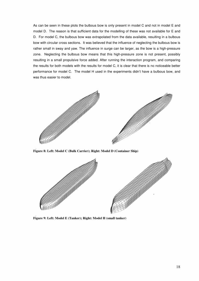
18

As can be seen in these plots the bulbous bow is only present in model C and not in model E and

model D. The reason is that sufficient data for the modelling of these was not available for E and

D. For model C, the bulbous bow was extrapolated from the data available, resulting in a bulbous

bow with circular cross sections. It was believed that the influence of neglecting the bulbous bow is

rather small in sway and yaw. The influence in surge can be larger, as the bow is a high-pressure

zone. Neglecting the bulbous bow means that this high-pressure zone is not present, possibly

resulting in a small propulsive force added. After running the interaction program, and comparing

the results for both models with the results for model C, it is clear that there is no noticeable better

performance for model C. The model H used in the experiments didn’t have a bulbous bow, and

was thus easier to model.

x

y

x

Figure 8: Left: Model C (Bulk Carrier); Right: Model D (Container Ship)

x

y

x

Figure 9: Left: Model E (Tanker); Right: Model H (small tanker)

19

x

y

z

Figure 10: Typical configuration: Model C (left) taking over model E (right), containing 1798 panels in

total

20

Chapter 6: Comparison Parameters The experiments were always executed with two ships from which the centerplanes were parallel.

Most experiments were executed with clearances of, or half the beam of the target ship, or half the

beam of the own ship. The exact value is given in chapter 7 were the comparisons are shown.

Only in a few specific cases larger or smaller clearances are used.

6.1 Water Depths The standard water depths are written down in table 5. The water depths are only in two cases

different from the standard water depth, namely the two encounter cases between model E and

model D, in which the water depths are respectively 17.08 meters and 23.04 meters.

OWN T0

D E H

13.50 15.53 13.35

TA

RG

ET

Tt

C

13.50 17.08 18.63 17.08

D

13.50 X

17.08

18.63 18.63

23.04

E

15.53 18.63 X 18.63

H

9.38 17.08 18.63 X

Table 5: Standard water depths (in bolt) and standard drafts. The values in the table denote the water

depth h

6.2 Coordinate Systems Vantorre et al.(2002) use a ship fixed coordinate system, depending from which side the target ship

passes. Sutulo and Guedes Soares (2008) use a standard body-fixed coordinate system,

independent of the target ship. This had as a consequence that bad positioning of the ships would

require transformations between both coordinate systems.

The system used by Vantorre is:

• X’ Dimensionless longitudinal force: Positive if forward

• Y’ Dimensionless lateral force: Positive if repulsive

• N’ Dimensionless yaw moment: Positive if bow repulsed

A common used system, used by Sutulo, with a body-fixed frame is:

• X’ Dimensionless longitudinal force: Positive if forward

• Y’ Dimensionless lateral force: Positive to starboard side

• N’ Dimensionless yaw moment: Positive if clockwise (from sky perspective)

21

However, if simulations are done in this way that:

• The own ship takes over the target ship: The target ship is at port side of the own ship

• The target ship takes over the own ship: The own ship is at starboard side of the target

ship

• Encounter: Both ships are at port side with regard to each other

the coordinate systems from both will be equal. This is made clear in figures 11 to 13. This

standard setting is to keep the output files uniform and easier to process. There are two

exceptions for this standard setting. Both the exceptions are cases in which the same experiment

has been done twice, , so that data is available for both the target ship as for the own ship. In this

case the simulation only had to be run once. For these two cases (both encounter cases), an

additional file is added in the folder on the CD under the name “first column data.txt”.

6.3 Number of Mirrors Like mentioned before, the number of mirrors to simulate the bottom is four on each side.

6.4 Time Step The time step between the calculations is one second, for encounter as well as for overtake

manoeuvres. This number is chosen to maintain a good balance between accuracy and simulation

time. Overtake manoeuvres were simulated, depending on the situation, with a total time of more

or less 500 seconds. Encounter manoeuvres required around 250 seconds. Using a smaller time

step would have result in a considerable increase in simulation time. In section 7.6 the effect of

reducing the time step is examined.

22

Figure 11: Coordinate system for own ship taking over target ship used by Sutulo (left) and by

Vantorre (right)

Figure 12: Coordinate system for target ship taking over own ship used by Sutulo (left) and by

Vantorre (right)

Figure 13: Coordinate system for encounter cases used by Sutulo (left) and by Vantorre (right)

23

Chapter 7: Comparison Results The comparisons between the experimental data and the computational results are divided in three

cases:

• Forces measured on the overtaken ship

• Forces measured on the overtaking ship

• Encounter

The results for these situations are discussed separately in the next three sub-sections. The

number of panels equals the standard number of panels as mentioned in chapter 5. In total, 62

comparisons are performed for these standard models. Because they can not be plotted all, only

the most interesting results will be plotted and discussed in this thesis. The other ones are

available on the CD.

The results are always plotted in three graphs: surge, sway and yaw. The interaction code is a

potential flow code meaning that the ship’s proper resistive force is zero. The real value differs

slightly due to errors originating in numerical calculation methods used. Also the experimental data

was available with the proper resistive force of the ship already subtracted. In the comparisons

represented further on are thus only the added propulsive or resistive forces due to the interaction

effects present in the surge force.

Coordinates for longitudinal distance and transverse clearance are as follows (figure 14): ξ’ longitudinal distance between the midship sections from the own and the target ship,

divided by (LO + LT)/2, increasing with time in any manoeuvre

ybb clearance between the ships (in metres)

TARGET

OWN

yo

xo

LT

BT

ybbycc ycb

yooyoT

1

2(L o +L T )

L o

Bo

To

TT

h

Vo VT Figure 14: Conventions and symbols (from: Vantorre et Al. (2002))

The own ship is the ship on which the forces are measured. Computational results are available

for both the target and the own ship. The experimental results are only available for the own ship.

Therefore comparisons are only plotted for the own ship.

24

The process is unsteady since a relative speed between both ships exist and is as such calculated

by the computational code for the following sub-sections.

The calculation time was very difficult to predict. Since the simulations were run on different

computers with different specifications it is not possible to compare these times. But also between

simulations run on the same computer, a small change in a single parameter (for instance the

water depth) could double the calculating time. On the other hand, reducing the number of panels

gave a noticeable decrease in calculating time.

The final results are not compared in a mathemathical way. To overcome this, a division is made

for the results, based on the visual results:

• No agreement

• Qualitative agreement: the same shape, but not the same values

• Quantitative agreement: the same shape and the same values

There are only three possible classifications, because evaluation of the graphs on sight is very

arbitrary. But even then, it is sometimes hard to classify certain cases. For example a graph

containing two peaks from which one gives complete accordance, but the other one only partly can

be assigned as qualitative agreement. But it can also be assigned as quantitative agreement when

the peak which only partly agrees, is a lot smaller. Therefore this classification can not be used as

a strict classification but is used to give an idea of the global results of the comparisons.

7.1 The Own Ship takes over the Target Ship The 14 comparisons executed are given in table 6. The speeds are always 12 knots for the

overtaking ship and 8 for the overtaken ship. Like mentioned before this might be to fast to use only

potential flow code, but as seen further on, some good results are obtained. The drafts and the

water depths are the standard values as mentioned in chapter 6. In table 7 all the absolute values

are made dimensionless in the way explained in chapter 4.

In all graphs the horizontal axis is the dimensionless longitudinal distance between both ships. The

vertical axis is the dimensionless force component. Subscript “n” stands for “numerical” and are

the computational results (solid line). Subscript “e” stands for experimental results (dashed line

with squares).

The graphical results for the case when model H is overtaking model D is presented in figure 15.

In these graphs the numerical calculations approximate the best the experimental results.

25

Own Ship takes over Target Ship

Ships Speeds Drafts Clearance Depth

Own Target

Own (knots)

Target (knots)

Own (m)

Target (m)

ybb (m)

h (m)

1 D C 12 8 13.5 13.5 18.9 17.08

2 D E 12 8 13.5 15.53 20.63 18.63

3 D E 12 8 13.5 15.53 10.31 18.63

4 D E 12 8 13.5 15.53 41.25 18.63

5 D E 12 8 13.5 15.53 82.5 18.63

6 D E 12 8 13.5 15.53 123.75 18.63

7 D E 12 8 13.5 15.53 165 18.63

8 D H 12 8 13.5 9.38 11.1 17.08

9 E C 12 8 15.53 13.5 18.9 18.63

10 E D 12 8 15.53 13.5 20.63 18.63

11 E H 12 8 15.53 9.38 11.1 18.63

12 H C 12 8 13.35 13.5 18.9 17.08

13 H D 12 8 13.35 13.5 20.63 17.08

14 H E 12 8 13.35 15.53 23.4 18.63

Table 6: Performed Comparisons for own ship taking over the target ship

Parameters Dimensionless Parameters

Ships Speeds Depth Froude Nr Speed Transverse Distance

Own Target

Own (knots)

Target (knots)

own Target Own

length Target length

Depth h Own/

Target η'

1 D C 12 8 1.27 1.27 0.10 0.10 0.42 1.50 1.48

2 D E 12 8 1.38 1.20 0.10 0.10 0.40 1.50 1.47

3 D E 12 8 1.38 1.20 0.10 0.10 0.40 1.50 1.23

4 D E 12 8 1.38 1.20 0.10 0.10 0.40 1.50 1.94

5 D E 12 8 1.38 1.20 0.10 0.10 0.40 1.50 2.87

6 D E 12 8 1.38 1.20 0.10 0.10 0.40 1.50 3.81

7 D E 12 8 1.38 1.20 0.10 0.10 0.40 1.50 4.75

8 D H 12 8 1.27 1.82 0.10 0.14 0.42 1.50 1.35

9 E C 12 8 1.20 1.38 0.10 0.10 0.40 1.50 1.45

10 E D 12 8 1.20 1.38 0.10 0.10 0.40 1.50 1.47

11 E H 12 8 1.20 1.99 0.10 0.14 0.40 1.50 1.32

12 H C 12 8 1.28 1.27 0.14 0.10 0.42 1.50 1.63

13 H D 12 8 1.28 1.27 0.14 0.10 0.42 1.50 1.65

14 H E 12 8 1.40 1.20 0.14 0.10 0.40 1.50 1.68

Table 7: Performed comparisons for own ship taking over target ship, dimensionless

An other interesting result is shown in figure 16. These graphs represent the results for model H

taking over model C. The computational surge force has a different shape and shows a local

minimum followed by a local maximum when the midships are aligned. This twist is not present in

the experimental result, which has more or less the same shape as when H is overtaking D.

26

ξ′s,n

, ξ′s,e

-1.5 -1 -0.5 0 0.5 1 1.5-0.025

-0.02

-0.015

-0.01

-0.005

0

0.005

0.01

0.015

0.02

X′n

X′e

ξ′s,n

, ξ′s,e

-1.5 -1 -0.5 0 0.5 1 1.5-0.08

-0.06

-0.04

-0.02

0

0.02

0.04

0.06

Y′n

Y′e

ξ′s,n

, ξ′s,e

-1.5 -1 -0.5 0 0.5 1 1.5-0.03

-0.025

-0.02

-0.015

-0.01

-0.005

0

0.005

0.01

0.015

0.02

0.025

0.03

N′n

N′e

Figure 15: Model H taking over model D

ξ′s,n

, ξ′s,e

-1.5 -1 -0.5 0 0.5 1 1.5-0.035

-0.03

-0.025

-0.02

-0.015

-0.01

-0.005

0

0.005

0.01

0.015

0.02

X′n

X′e

ξ′s,n

, ξ′s,e

-1.5 -1 -0.5 0 0.5 1 1.5-0.15

-0.1

-0.05

0

0.05

0.1

0.15

Y′n

Y′e

ξ′s,n

, ξ′s,e

-1.5 -1 -0.5 0 0.5 1 1.5-0.04

-0.02

0

0.02

0.04

0.06

N′n

N′e

Figure 16: Model H taking over model C

In figure 17 and figure 18 are two more comparisons shown from the cases with the relative best

results, namely model D taking over model C and model D taking over model H. In which the first

is a comparison of two ships with more or less the same length and the second is a comparison of

two ships of significant different length.

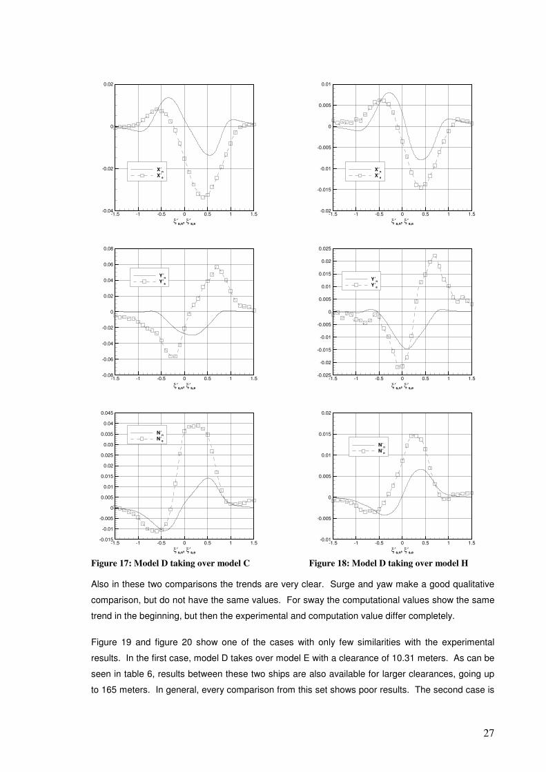
27

ξ′s,n

, ξ′s,e

-1.5 -1 -0.5 0 0.5 1 1.5-0.04

-0.02

0

0.02

X′n

X′e

ξ′s,n

, ξ′s,e

-1.5 -1 -0.5 0 0.5 1 1.5-0.08

-0.06

-0.04

-0.02

0

0.02

0.04

0.06

0.08

Y′n

Y′e

ξ′s,n

, ξ′s,e

-1.5 -1 -0.5 0 0.5 1 1.5-0.015

-0.01

-0.005

0

0.005

0.01

0.015

0.02

0.025

0.03

0.035

0.04

0.045

N′n

N′e

Figure 17: Model D taking over model C

ξ′s,n

, ξ′s,e

-1.5 -1 -0.5 0 0.5 1 1.5-0.02

-0.015

-0.01

-0.005

0

0.005

0.01

X′n

X′e

ξ′s,n

, ξ′s,e

-1.5 -1 -0.5 0 0.5 1 1.5-0.025

-0.02

-0.015

-0.01

-0.005

0

0.005

0.01

0.015

0.02

0.025

Y′n

Y′e

ξ′s,n

, ξ′s,e

-1.5 -1 -0.5 0 0.5 1 1.5-0.01

-0.005

0

0.005

0.01

0.015

0.02

N′n

N′e

Figure 18: Model D taking over model H

Also in these two comparisons the trends are very clear. Surge and yaw make a good qualitative

comparison, but do not have the same values. For sway the computational values show the same

trend in the beginning, but then the experimental and computation value differ completely.

Figure 19 and figure 20 show one of the cases with only few similarities with the experimental

results. In the first case, model D takes over model E with a clearance of 10.31 meters. As can be

seen in table 6, results between these two ships are also available for larger clearances, going up

to 165 meters. In general, every comparison from this set shows poor results. The second case is

28

model E taking over model C. Here there is only few accordance in yaw. Surge shows only minor

resemblance and the sway force shows no resemblance. The results for the computational surge

force are quite unique in this case, showing no explicit peaks in the force.

ξ′s,n

, ξ′s,e

-1.5 -1 -0.5 0 0.5 1 1.5-0.06

-0.04

-0.02

0

0.02

0.04

X′n

X′e

ξ′s,n

, ξ′s,e

-1.5 -1 -0.5 0 0.5 1 1.5-0.08

-0.06

-0.04

-0.02

0

0.02

0.04

0.06

Y′n

Y′e

ξ′s,n

, ξ′s,e

-1.5 -1 -0.5 0 0.5 1 1.5-0.02

0

0.02

0.04

0.06

N′n

N′e

Figure 19: Model D taking over model E with

10.31 metres of clearance

ξ′s,n

, ξ′s,e

-1.5 -1 -0.5 0 0.5 1 1.5-0.06

-0.04

-0.02

0

0.02

X′n

X′e

ξ′s,n

, ξ′s,e

-1.5 -1 -0.5 0 0.5 1 1.5-0.15

-0.1

-0.05

0

0.05

0.1

0.15

Y′n

Y′e

ξ′s,n

, ξ′s,e

-1.5 -1 -0.5 0 0.5 1 1.5-0.06

-0.04

-0.02

0

0.02

0.04

0.06

0.08

N′n

N′e

Figure 20: Model E taking over model C

The six comparisons illustrated before show some trends, which is also present in the other figures

not presented in this thesis, but available on the CD.

29

Using the division method based on the quantitative and qualitative division, table 8 is obtained for

these cases. In which the symbols have following meaning:

X No agreement

V Qualitative agreement

VV Quantitative agreement

As the table shows, agreement for sway is always mean. Neither the values, nor the shapes agree

with the experimental results. For surge some good results are obtained as well as for yaw. These

good results are obtained in the last three cases, when model H, being a lot smaller then the other

ships, is taking over the other three models. An other remark is that the yaw force shows

especially disagreement in the cases where model D takes over model E.

Own Ship takes over Target Ship

Ships Speeds Clearance Results

Own Target

Own (knots)

Target (knots)

ybb (m)

surge sway yaw

1 D C 12 8 18.9 V X V

2 D E 12 8 20.63 V X X

3 D E 12 8 10.31 V X X

4 D E 12 8 41.25 V X X

5 D E 12 8 82.5 V X X

6 D E 12 8 123.75 V X X

7 D E 12 8 165 V X X

8 D H 12 8 11.1 V X V

9 E C 12 8 18.9 X X V

10 E D 12 8 20.63 V X V

11 E H 12 8 11.1 X X V

12 H C 12 8 18.9 V X VV

13 H D 12 8 20.63 VV X VV

14 H E 12 8 23.4 V X VV

No. of X 2 14 6

No. of V 11 0 5

No. of VV 1 0 3

Total 14 14 14

Table 8: Comparisons for the own ship taking over the target ship: evaluation

7.1.1 Surge According to the computational results, when ξ is more or less -1, the ship undergoes a small

resistive force, followed by an extra propulsive force which reaches a peak between -0.5 and -0.3.

This peak is followed by a quick decrease of the propulsive force, with sometimes a local minimum

and maximum around 0 like in figure 16. Subsequently the ship undergoes an additional resistive

force. When ξ is more or less 1, once again a small propulsive force is generated followed by a

30

return to zero of the surge force. For all cases the results from the computational results show a

symmetry around the origin.

The experimental results show the same trends. The small resistive force and the small propulsive

force in the beginning and end are mostly not present. The resistive and propulsive peaks are

present, but with the resistive peak in most cases a lot larger than the propulsive peak. This makes

that in general the propulsive peak is overestimated by the computer code, and the resistive peak

underestimated.

7.1.2 Sway The sway forces show for all these cases a very bad accordance. The computational sway force

shows only a strong attractive force. With sometimes a slight reduction from the attraction force

when the amidships are aligned. Like the surge force, there is some symmetry present, but this

time around the vertical axis.

The experimental results however show more a symmetry around the origin. They show a peak in

the attractive force between -0.5 and -0.3 followed by a climb to a repulsive peak between 0.5 and

0.8. The absolute value of both peaks is in most cases quite equal. The repulsive peak is nowhere

present in the computational data. Also the attractive peak is in most cases underestimated.

7.1.3 Yaw The computational yaw results are characterised by an attractive force on the bow towards the ship

which is being overtaken. Followed by a strong repulsive force on the bow in the second part of the

manoeuvre (after the amidships sections have been aligned). The two peaks have in most cases

more or less the same absolute value.

The behaviour of the plots in the experimental results resembles the computation results, with this

difference that in some cases the repulsive bow force in the second part of the manoeuvre is a lot

stronger then the attractive force in the first part.

In most cases, the comparison results are good in the first (attractive) peak. When the experimental

results are approximately symmetric around the origin, the comparison is also good for the second

peak (see figures 15 and 16). If this symmetry is not present, the second (repulsive) peak is mostly

a lot stronger in the experimental results (figures 17, 18 and 19). In two cases, there is a scaling

discrepancy for both peaks, when model E is taking over model C (figure 20) and when model E is

taking over model D (on the CD).

7.2 The Target Ship takes over the Own Ship In the following cases, measurements are made on the ship which is being overtaken (the own

ship). The target ship has always a speed of 12 knots and a clearance and water depth depending

on the situation. The own ship has in most cases a speed of 8 knots, except for one case

31

resembling a moored ship (0 knots) and one case at low speed (4 knots). All this data is

summarized in table 9 and dimensionless in table 10.

Target Ship takes over Own Ship

Ships Speeds Drafts Clearance Depth

Own Target

Own (knots)

Target (knots)

Own (m)

Target (m)

ybb (m)

h (m)

1 D C 8 12 13.5 13.5 18.9 17.08

2 D E 8 12 13.5 15.53 20.63 18.63

3 D E 8 12 13.5 15.53 10.31 18.63

4 D E 8 12 13.5 15.53 41.25 18.63

5 D E 8 12 13.5 15.53 82.5 18.63

6 D E 8 12 13.5 15.53 123.75 18.63

7 D E 8 12 13.5 15.53 165 18.63

8 D H 8 12 13.5 9.38 11.1 17.08

9 E D 0 12 15.53 13.5 20.63 18.63

10 E D 4 12 15.53 13.5 20.63 18.63

11 E C 8 12 15.53 13.5 18.9 18.63

12 E D 8 12 15.53 13.5 20.63 18.63

13 E H 8 12 15.53 9.38 11.1 18.63

14 H C 8 12 13.35 13.5 18.9 17.08

15 H D 8 12 13.35 13.5 20.63 17.08

16 H E 8 12 13.35 15.53 23.4 18.63

Table 9: Performed comparisons for the target ship taking over the own ship

Parameters Dimensionless Parameters

Ships Speeds Depth Froude Nr Speed

Transverse Distance

Own Target

Own (knots)

Target (knots)

own Target Own

length Target length

Depth h Own/

Target η'

1 D C 8 12 1.27 1.27 0.10 0.10 0.42 0.67 1.48

2 D E 8 12 1.38 1.20 0.10 0.10 0.40 0.67 1.47

3 D E 8 12 1.38 1.20 0.10 0.10 0.40 0.67 1.23

4 D E 8 12 1.38 1.20 0.10 0.10 0.40 0.67 1.94

5 D E 8 12 1.38 1.20 0.10 0.10 0.40 0.67 2.87

6 D E 8 12 1.38 1.20 0.10 0.10 0.40 0.67 3.81

7 D E 8 12 1.38 1.20 0.10 0.10 0.40 0.67 4.75

8 D H 8 12 1.27 1.82 0.10 0.14 0.42 0.67 1.35

9 E D 0 12 1.20 1.38 0.12 0.12 0.46 0.00 1.47

10 E D 4 12 1.20 1.38 0.10 0.10 0.40 0.33 1.47

11 E C 8 12 1.20 1.38 0.10 0.10 0.40 0.67 1.45

12 E D 8 12 1.20 1.38 0.10 0.10 0.40 0.67 1.47

13 E H 8 12 1.20 1.99 0.10 0.14 0.40 0.67 1.32

14 H C 8 12 1.28 1.27 0.14 0.10 0.42 0.67 1.63

15 H D 8 12 1.28 1.27 0.14 0.10 0.42 0.67 1.65

16 H E 8 12 1.40 1.20 0.14 0.10 0.40 0.67 1.68

Table 10: Performed comparisons for the target ship taking over the own ship, dimensionless

32

In figure 21 model H is overtaken by model D (large ship taking over a small ship). This case

shows the most resemblance between computational and experimental results, from the cases in

table 9.

Figure 22 shows the effect of a large ship being taken over by a smaller ship, namely model D

being overtaken by model H. This is also one of the best results from the cases in table 9.

ξ′s,n

, ξ′s,e

-2 -1.5 -1 -0.5 0 0.5 1 1.5 2-0.06

-0.04

-0.02

0

0.02

0.04 X′n

X′e

ξ′s,n

, ξ′s,e

-2 -1.5 -1 -0.5 0 0.5 1 1.5 2-0.14

-0.12

-0.1

-0.08

-0.06

-0.04

-0.02

0

0.02

0.04

0.06

0.08

0.1

Y′n

Y′e

ξ′s,n

, ξ′s,e

-2 -1.5 -1 -0.5 0 0.5 1 1.5 2-0.06

-0.04

-0.02

0

0.02

0.04

N′n

N′e

Figure 21: Model H taken over by model D

ξ′s,n

, ξ′s,e

-2 -1.5 -1 -0.5 0 0.5 1 1.5 2-0.03

-0.025

-0.02

-0.015

-0.01

-0.005

0

0.005

0.01

0.015

0.02

X′n

X′e

ξ′s,n

, ξ′s,e

-2 -1.5 -1 -0.5 0 0.5 1 1.5 2-0.06

-0.04

-0.02

0

0.02

0.04

Y′n

Y′e

ξ′s,n

, ξ′s,e

-2 -1.5 -1 -0.5 0 0.5 1 1.5 2-0.015

-0.01

-0.005

0

0.005

0.01

0.015

0.02

0.025

0.03

N′n

N′e

Figure 22: Model D taken over by model H

33

More two situations are given in figures 23 and 24. The first one represents model E being

overtaken by model H. This case shows no good quantitative agreement but the graphs do have a

very similar shape (especially for sway and yaw). The computational surge force shows, like in

some of the cases where the own ship was overtaking, a local minimum and maximum, which are

not present in the experimental data.

The second one represents model E going at 4 knots, being overtaken by model D at 12 knots.

ξ′s,n

, ξ′s,e

-2 -1.5 -1 -0.5 0 0.5 1 1.5 2-0.03

-0.025

-0.02

-0.015

-0.01

-0.005

0

0.005

0.01

0.015

0.02

0.025

X′n

X′e

ξ′s,n

, ξ′s,e

-2 -1.5 -1 -0.5 0 0.5 1 1.5 2-0.1

-0.08

-0.06

-0.04

-0.02

0

0.02

0.04

0.06

Y′n

Y′e

ξ′s,n

, ξ′s,e

-2 -1.5 -1 -0.5 0 0.5 1 1.5 2-0.04

-0.03

-0.02

-0.01

0

0.01

0.02

0.03

0.04

N′n

N′e

Figure 23: Model E taken over by model H

ξ′s,n

, ξ′s,e

-2 -1.5 -1 -0.5 0 0.5 1 1.5 2-0.06

-0.05

-0.04

-0.03

-0.02

-0.01

0

0.01

0.02

0.03

0.04

0.05

X′n

X′e

ξ′s,n

, ξ′s,e

-2 -1.5 -1 -0.5 0 0.5 1 1.5 2-0.14

-0.12

-0.1

-0.08

-0.06

-0.04

-0.02

0

0.02

0.04

0.06

0.08

0.1

0.12

Y′n

Y′e

ξ′s,n

, ξ′s,e

-2 -1.5 -1 -0.5 0 0.5 1 1.5 2-0.04

-0.03

-0.02

-0.01

0

0.01

0.02

0.03

0.04

0.05

N′n

N′e

Figure 24: Model E (4 knots) taken over by

model D

34

The two following situations shown (figures 25 and 26) coincide a lot less. In these cases, ship D

was overtaken by ship E. In the first graph with a very small clearance (10.31 metres), in the

second graph with a rather large clearance with respect to the other cases (41.25 metres).

ξ′s,n

, ξ′s,e

-1.5 -1 -0.5 0 0.5 1 1.5-0.1

-0.05

0

0.05

X′n

X′e

ξ′s,n

, ξ′s,e

-1.5 -1 -0.5 0 0.5 1 1.5-0.15

-0.1

-0.05

0

0.05

0.1

0.15

Y′n

Y′e

ξ′s,n

, ξ′s,e

-1.5 -1 -0.5 0 0.5 1 1.5-0.06

-0.04

-0.02

0

0.02

0.04

0.06

0.08

N′n

N′e

Figure 25: Model D taken over by model E

with 10.31 metres of clearance

ξ′s,n

, ξ′s,e

-1.5 -1 -0.5 0 0.5 1 1.5-0.06

-0.04

-0.02

0

0.02

0.04

X′n

X′e

ξ′s,n

, ξ′s,e

-1.5 -1 -0.5 0 0.5 1 1.5-0.08

-0.06

-0.04

-0.02

0

0.02

0.04

0.06

0.08

0.1

Y′n

Y′e

ξ′s,n

, ξ′s,e

-1.5 -1 -0.5 0 0.5 1 1.5-0.04

-0.02

0

0.02

0.04

0.06

N′n

N′e

Figure 26: Model D taken over by model E

with 41.25 metres of clearance

Figure 27 shows E taken over by C, also this comparison shows strong discrepancies between

computational and experimental data.

35

ξ′s,n

, ξ′s,e

-1.5 -1 -0.5 0 0.5 1 1.5-0.08

-0.06

-0.04

-0.02

0

0.02

0.04

0.06

X′n

X′e

ξ′s,n

, ξ′s,e

-1.5 -1 -0.5 0 0.5 1 1.5-0.15

-0.1

-0.05

0

0.05

0.1

0.15

Y′n

Y′e

ξ′s,n

, ξ′s,e

-1.5 -1 -0.5 0 0.5 1 1.5-0.08

-0.06

-0.04

-0.02

0

0.02

0.04

0.06

0.08

N′n

N′e

Figure 27: Model E taken over by model C

Using the same system as before, table 11 was obtained for the comparison results.

36

The results for these cases (own ship overtaken) are slightly better then in the previous cases (own

ship is overtaking). Surge and yaw show a lot of qualitative good results with a few quantitative

good results as well. Sway comparisons still show a lot of discrepancies, but some better results

are also obtained. Noticeable is also that most of the good results obtained are from cases which

involve the smaller ship H.

Target Ship takes over Own Ship

Ships Speeds Clearance Results

Own Target

Own (knots)

Target (knots)

ybb (m)

surge sway yaw

1 D C 8 12 18.9 V X V

2 D E 8 12 20.63 V X X

3 D E 8 12 10.31 V X X

4 D E 8 12 41.25 V X X

5 D E 8 12 82.5 V X X

6 D E 8 12 123.75 X X V

7 D E 8 12 165 X X X

8 D H 8 12 11.1 VV V V

9 E D 0 12 20.63 V V V

10 E D 4 12 20.63 V V V

11 E C 8 12 18.9 X X V

12 E D 8 12 20.63 V X V

13 E H 8 12 11.1 V V V

14 H C 8 12 18.9 V X VV

15 H D 8 12 20.63 VV VV VV

16 H E 8 12 23.4 V X VV

No. of X 3 11 5

No. of V 11 4 8

No. of VV 2 1 3

Total 16 16 16

Table 11: Comparisons for target ship taking over the own ship: evaluation

7.2.1 Surge In the surge case both the computational data as the experimental data show at first a peak of an

additional resistance force, followed by a peak of an additional propulsive force. For the

computational data the absolute values for both peaks are more or less equal. In the experimental

data the resistance peak is mostly larger then the propulsive peak. Comparing computational with

experimental, there is mostly an underestimation of the first peak and a more or less equal result

for the second peak.

7.2.2 Sway For the sway force there is an initial small peak of repulsion, followed by a large peak of attraction,

followed by repulsion once again. Like in surge, the computational results are much more

symmetric showing two equal peaks of repulsion. In the experimental results this first repulsive

37

peak is mostly a lot larger. In general the computational values of the attractive peaks are quite

close to the experimental value. The shape of the graph however, and the value of the first peak

are mostly not equal.

7.2.3 Yaw Sway results show at first that the bow is repulsed, followed by an attractive moment. The trend for

these comparisons is the same as for sway and surge, namely that both peaks in the

computational results have almost an equal absolute value. In contrary to the experimental results

in which the first peak has a larger value. This makes that the computational value for the first

peak is underestimated, but that the value for the second peak is mostly quite equal.

7.3 Encounter The number of encounter cases is larger then in previous sections, they are listed in table 12 and in

dimensionless form in table 13.

38

ENCOUNTER

Ships Speeds Drafts Clearance Depth

Own Target Own

(knots) Target (knots)

Own (m)

Target (m)

ybb (m)

h (m)

1 D E 8 8 13.5 15.53 20.63 18.63

2 D E 8 8 13.5 15.53 10.31 18.63

3 D E 8 8 13.5 15.53 41.25 18.63

4 D E 8 8 13.5 15.53 82.5 18.63

5 D E 8 8 13.5 15.53 123.75 18.63

6 D E 8 8 13.5 15.53 165 18.63

7 D E 8 8 13.5 15.53 206.25 18.63

8 D C 12 0 13.5 13.5 18.9 17.08

9 D C 12 12 13.5 13.5 18.9 17.08

10 D E 12 0 13.5 15.53 20.63 18.63

11 D E 12 12 13.5 15.53 20.63 18.63

12 D H 12 12 13.5 9.38 11.1 17.08

13 E D 0 8 15.53 13.5 20.63 18.63

14 E D 4 8 15.53 13.5 20.63 18.63

15 E D 8 0 15.53 13.5 20.63 18.63

16 E D 8 4 15.53 13.5 20.63 18.63

17 E D 8 8 15.53 13.5 20.63 18.63

18 E D 8 12 15.53 13.5 20.63 18.63

19 E C 12 0 15.53 13.5 18.9 18.63

20 E C 12 12 15.53 13.5 18.9 18.63

21 E D 12 8 15.53 13.5 20.63 18.63

22 E D 12 12 15.53 13.5 20.63 18.63

23 E D 12 12 15.53 13.5 20.63 17.08

24 E D 12 12 15.53 13.5 20.63 23.04

25 E H 12 12 15.53 9.38 11.1 18.63

26 H C 8 0 13.35 13.5 18.9 17.08

27 H C 8 4 13.35 13.5 18.9 17.08

28 H C 8 8 13.35 13.5 18.9 17.08

29 H C 8 12 13.35 13.5 18.9 17.08

30 H C 12 12 13.35 13.5 18.9 17.08

31 H D 12 12 13.35 13.5 20.63 18.63

32 H E 12 12 13.35 15.53 23.4 18.63

Table 12: Performed comparisons for encounter

39

Parameters Dimensionless Parameters

Ships Speeds Depth Froude Nr Speed Transverse

Distance

Own Target

Own (knots)

Target (knots)

own Target Own

length Target length

Depth h Own/

Target η'

1 D E 8 8 1.38 1.20 0.077 0.078 0.30 1.00 1.47

2 D E 8 8 1.38 1.20 0.077 0.078 0.30 1.00 1.23

3 D E 8 8 1.38 1.20 0.077 0.078 0.30 1.00 1.94

4 D E 8 8 1.38 1.20 0.077 0.078 0.30 1.00 2.87

5 D E 8 8 1.38 1.20 0.077 0.078 0.30 1.00 3.81

6 D E 8 8 1.38 1.20 0.077 0.078 0.30 1.00 4.75

7 D E 8 8 1.38 1.20 0.077 0.078 0.30 1.00 5.68

8 D C 12 0 1.27 1.27 0.116 0.114 0.48 ∞ 1.48

9 D C 12 12 1.27 1.27 0.116 0.114 0.48 1.00 1.48

10 D E 12 0 1.38 1.20 0.116 0.116 0.46 ∞ 1.47

11 D E 12 12 1.38 1.20 0.116 0.116 0.46 1.00 1.47

12 D H 12 12 1.27 1.82 0.116 0.153 0.48 1.00 1.35

13 E D 0 8 1.20 1.38 0.078 0.077 0.30 0 1.47

14 E D 4 8 1.20 1.38 0.067 0.067 0.26 0.50 1.47

15 E D 8 0 1.20 1.38 0.078 0.077 0.30 ∞ 1.47

16 E D 8 4 1.20 1.38 0.067 0.067 0.26 2.00 1.47

17 E D 8 8 1.20 1.38 0.078 0.077 0.30 1.00 1.47

18 E D 8 12 1.20 1.38 0.103 0.102 0.40 0.67 1.47

19 E C 12 0 1.20 1.38 0.116 0.114 0.46 ∞ 1.45

20 E C 12 12 1.20 1.38 0.116 0.114 0.46 1.00 1.45

21 E D 12 8 1.20 1.38 0.103 0.102 0.40 1.50 1.47

22 E D 12 12 1.20 1.38 0.116 0.116 0.46 1.00 1.47

23 E D 12 12 1.10 1.27 0.116 0.116 0.48 1.00 1.47

24 E D 12 12 1.48 1.71 0.116 0.116 0.41 1.00 1.47

25 E H 12 12 1.20 1.99 0.116 0.153 0.46 1.00 1.32

26 H C 8 0 1.28 1.27 0.102 0.076 0.32 ∞ 1.63

27 H C 8 4 1.28 1.27 0.088 0.066 0.28 2.00 1.63

28 H C 8 8 1.28 1.27 0.102 0.076 0.32 1.00 1.63

29 H C 8 12 1.28 1.27 0.135 0.101 0.42 0.67 1.63

30 H C 12 12 1.28 1.27 0.153 0.114 0.48 1.00 1.63

31 H D 12 12 1.40 1.38 0.153 0.116 0.46 1.00 1.65

32 H E 12 12 1.40 1.20 0.153 0.116 0.46 1.00 1.68

Table 13: Performed comparisons for encounter: dimensionless

The different situations covered in the encounter cases are more various then the overtake cases:

the speeds vary between 0 and 12 knots and more combinations at different speed are made. In

the case of two ships encountering both at 12 knots, surface effects can have a strong influence on

the interaction forces.

40

One of the best results is model E encountering model D, in which E is the own ship going at 4

knots, and D goes at 8 knots. Results are given in figure 28. The second case shown (figure 29) is

model H encountering model C, respectively at 8 and 12 knots.

ξ′s,n

, ξ′s,e

-1.5 -1 -0.5 0 0.5 1 1.5-0.04

-0.02

0

0.02

0.04

X′n

X′e

ξ′s,n

, ξ′s,e

-1.5 -1 -0.5 0 0.5 1 1.5-0.3

-0.25

-0.2

-0.15

-0.1

-0.05

0

0.05

0.1

0.15

Y′n

Y′e

ξ′s,n

, ξ′s,e

-1.5 -1 -0.5 0 0.5 1 1.5-0.06

-0.04

-0.02

0

0.02

0.04

N′n

N′e

Figure 28: Model E (own ship) at 4 knots

encountering model D at 8 knots

ξ′s,n

, ξ′s,e

-1.5 -1 -0.5 0 0.5 1 1.5-0.04

-0.02

0

0.02

0.04

0.06

X′n

X′e

ξ′s,n

, ξ′s,e

-1.5 -1 -0.5 0 0.5 1 1.5-0.3

-0.25

-0.2

-0.15

-0.1

-0.05

0

0.05

0.1

0.15

0.2

0.25

Y′n

Y′e

ξ′s,n

, ξ′s,e

-1.5 -1 -0.5 0 0.5 1 1.5-0.06

-0.04

-0.02

0

0.02

0.04

N′n

N′e

Figure 29: Model H (own ship) at 8 knots

encountering model C at 12 knots

Other good results are given in figures 30 and 31. The first case is model E encountering model H,

both at twelve knots, with E the own ship. The experimental values for the surge force are

distorted by noise, but the trend is clear. The second comparison is model E (own ship)

encountering model D, both at 8 knots.

41

ξ′s,n

, ξ′s,e

-1.5 -1 -0.5 0 0.5 1 1.5-0.02

-0.015

-0.01

-0.005

0

0.005

0.01

0.015

0.02

X′n

X′e

ξ′s,n

, ξ′s,e

-1.5 -1 -0.5 0 0.5 1 1.5-0.15

-0.1

-0.05

0

0.05

0.1

0.15

Y′n

Y′e

ξ′s,n

, ξ′s,e

-1.5 -1 -0.5 0 0.5 1 1.5-0.06

-0.04

-0.02

0

0.02

0.04

N′n

N′e

Figure 30: Model E (own ship) at 12 knots

encountering model H at 12 knots

ξ′s,n

, ξ′s,e

-2 -1.5 -1 -0.5 0 0.5 1 1.5 2-0.03

-0.02

-0.01

0

0.01

0.02

0.03

0.04

X′n

X′e

ξ′s,n

, ξ′s,e

Y′ n

,Y

′ e

-2 -1.5 -1 -0.5 0 0.5 1 1.5 2-0.3

-0.25

-0.2

-0.15

-0.1

-0.05

0

0.05

0.1

0.15

0.2

Y′n

Y′e

ξ′s,n

, ξ′s,e

-2 -1 0 1 2-0.04

-0.03

-0.02

-0.01

0

0.01

0.02

0.03

0.04

N′n

N′e

Figure 31: Model E (own ship) at 8 knots

encountering model D at 8 knots

Large discrepancies are mostly present when the interaction forces are quite low. For instance in

the cases with a large clearance (165, 206, … meters) or in cases where the target ship has zero

speed. An example is shown in figure 32, where model D takes over model E, in which D (own

ship) goes at twelve knots and E at zero knots. Most other cases where the target ship has zero

speed are similar and show the same unconformity between experimental and computational data.

42

One of the least good comparisons (excluding the cases with zero target ship speed and large

clearance) is shown in figure 33. Model E is encountering model C, both at 12 knots. Although it is

one of the less good ones, the computational results are still quite good, and certainly a lot better

then some of the overtake comparisons.

ξ′s,n

, ξ′s,e

-1.5 -1 -0.5 0 0.5 1 1.5-0.01

-0.008

-0.006

-0.004

-0.002

0

0.002

0.004

X′n

X′e

ξ′s,n

, ξ′s,e

-1.5 -1 -0.5 0 0.5 1 1.5-0.05

-0.04

-0.03

-0.02

-0.01

0

0.01

0.02

Y′n

Y′e

ξ′s,n

, ξ′s,e

-1.5 -1 -0.5 0 0.5 1 1.5-0.004

-0.002

0

0.002

0.004

0.006

0.008

N′n

N′e

Figure 32: Model D (own ship) at 12 knots

encountering model E at 0 knots

ξ′s,n

, ξ′s,e

-1.5 -1 -0.5 0 0.5 1 1.5-0.06

-0.04

-0.02

0

0.02

0.04

X′n

X′e

ξ′s,n

, ξ′s,e

-1.5 -1 -0.5 0 0.5 1 1.5-0.5

-0.4

-0.3

-0.2

-0.1

0

0.1

0.2

0.3

Y′n

Y′e

ξ′s,n

, ξ′s,e

-1.5 -1 -0.5 0 0.5 1 1.5-0.04

-0.02

0

0.02

0.04

0.06

N′n

N′e

Figure 33: Model E (own ship) at 12 knots

encountering model C at 12 knots

A last case shows a very good agreement in the sway force. It is model H encountering with model

C, both at 8 knots.

43

ξ′s,n

, ξ′s,e

-1.5 -1 -0.5 0 0.5 1 1.5-0.03

-0.025

-0.02

-0.015

-0.01

-0.005

0

0.005

0.01

0.015

0.02

0.025

0.03

X′n

X′e

ξ′s,n

, ξ′s,e

-1.5 -1 -0.5 0 0.5 1 1.5-0.25

-0.2

-0.15

-0.1

-0.05

0

0.05

0.1

0.15

0.2

Y′n

Y′e

ξ′s,n

, ξ′s,e

-1.5 -1 -0.5 0 0.5 1 1.5-0.06

-0.04

-0.02

0

0.02

0.04

0.06

N′n

N′e

Figure 34: Model H (own ship) at 8 knots encountering model C at 8 knots

44

ENCOUNTER

Ships Speeds Clearance Results

Own Target

Own (knots)

Target (knots)

ybb (m)

surge sway yaw

1 D E 8 8 20.63 V V X

2 D E 8 8 10.31 VV V X

3 D E 8 8 41.25 V V V

4 D E 8 8 82.5 V V V

5 D E 8 8 123.75 V V V

6 D E 8 8 165 V V X

7 D E 8 8 206.25 X V X

8 D C 12 0 18.9 X X X

9 D C 12 12 18.9 V V V

10 D E 12 0 20.63 X X X

11 D E 12 12 20.63 VV V V

12 D H 12 12 11.1 VV V V

13 E D 0 8 20.63 VV V VV

14 E D 4 8 20.63 VV VV VV

15 E D 8 0 20.63 X X X

16 E D 8 4 20.63 X V V

17 E D 8 8 20.63 VV VV V

18 E D 8 12 20.63 VV V VV

19 E C 12 0 18.9 X X X

20 E C 12 12 18.9 X X V

21 E D 12 8 20.63 V V V

22 E D 12 12 20.63 VV V V

23 E D 12 12 20.63 VV V V

24 E D 12 12 20.63 V VV VV

25 E H 12 12 11.1 VV V VV

26 H C 8 0 18.9 X X X

27 H C 8 4 18.9 X VV VV

28 H C 8 8 18.9 V VV VV

29 H C 8 12 18.9 V VV VV

30 H C 12 12 18.9 V V VV

31 H D 12 12 20.63 V V VV

32 H E 12 12 23.4 V V VV

No. of X 9 6 9

No. of V 13 20 12

No. of VV 10 6 11

Total 32 32 32

Table 14: Comparisons for encounter: evaluation

In table 14 is shown that the results are in general a lot better for encounter then for overtake,

showing good agreement between computational and experimental data. A possible explanation

could be found in the Strouhal number. At large Strouhal numbers, viscosity dominates the flow

(Sobey, 1982). When using the relative speed between both ships as characteristic speed, it’s

45

clear that encounter manoeuvres result in smaller Strouhal numbers for encounter then for

overtake.

Drawing general conclusions for surge, sway and yaw is difficult because of the diversity in the

cases. Since the forces are very different when one of both ships has zero speed, following

conclusions will not cover these comparisons.

7.3.1 Surge For most cases, the surge force is increasing while approaching the oncoming ship, meaning that

an additional propulsive force is working on the ship. This is followed by a peak of additional

resistance force. For the experimental data, conclusions on the absolute values of the peaks are

not unambiguous, since sometimes the resistive peak is larger than the propulsive peak,

sometimes the other way around, or sometimes equal. For the computational data however, the

absolute value of both peaks is mostly equal.

An other remark is that the computational data shows in some cases a local minimum and

maximum around zero for the cases when model H is the own ship. These are not present in the

experimental data.

7.3.2 Sway Like in previous sub-section (The own ship overtaken by the target ship), the target ship shows a

repulsive force, followed by an attractive force, and again a repulsive force (with sometimes a local

maximum in the attractive force). Also here the first and second repulsive peaks are mostly equal

in the computational data. For the experimental data however, the peaks are a lot more symmetric

then in the overtake case, resulting in comparisons which match a lot better.

7.3.3 Yaw The yaw force differs depending on the ships involved and the speeds. Successive

periods of bow in and bow out moments are recognizable in the different figures.

In most cases, the own ship endures a bow out moment when approaching and a bow in moment

at the end of the encounter manoeuvre. Independent of the shape of the experimental results, the

different peaks of the yaw moment are calculated very accurately.

7.4 Steady versus Unsteady Taking over and encounter cases are in theory unsteady cases. However, if the relative speed

between both ships is small enough, the manoeuvre can also been seen as a steady manoeuvre.

In the following figures this difference is shown very clearly. The first graph (figure 35) is an

encounter case between model H (own ship) and model C (target ship), both at 8 knots. Figures

36 and 37 show respectively a comparison of model H (own ship) at 8 knots being taken over by

model C at 12 knots and model E (own ship) at 12 knots taking over model D at 8 knots.

46

For the encounter graphs it is clear that the steady results are worse than the unsteady. Probably

this is due to the larger relative speed between both ships.

The results for the overtake cases are more inconsistent. The two cases show that when model H

(own ship) is taken over by model C, the steady results are worse then the unsteady. But when

model E is taking over model D, the steady results show a better approximation then the unsteady

results.

ξ′s,unst

, ξ′s,e

, ξ′s,st

X'

-1.5 -1 -0.5 0 0.5 1 1.5-0.03

-0.025

-0.02

-0.015

-0.01

-0.005

0

0.005

0.01

0.015

0.02

0.025

0.03

SteadyExperimentalUnsteady

ξ′s,unst

, ξ′s,e

, ξ′s,st

Y'

-1.5 -1 -0.5 0 0.5 1 1.5-0.2

-0.15

-0.1

-0.05

0

0.05

0.1

0.15

0.2

0.25

Steady

ExperimentalUnsteady

ξ′s,unst

, ξ′s,e

, ξ′s,st

N'

-1.5 -1 -0.5 0 0.5 1 1.5-0.06

-0.04

-0.02

0

0.02

0.04

0.06

SteadyExperimentalUnsteady

Figure 35: Model H (own ship) at 8 knots encountering model C at 8 knots

47

ξ′s,unst

, ξ′s,e

, ξ′s,st

X'

-1.5 -1 -0.5 0 0.5 1 1.5-0.06

-0.04

-0.02

0

0.02

0.04

SteadyExperimentalUnsteady

ξ′s,unst

, ξ′s,e

, ξ′s,st

Y'

-1.5 -1 -0.5 0 0.5 1 1.5-0.15

-0.1

-0.05

0

0.05

0.1

0.15

0.2

SteadyExperimentalUnsteady

ξ′s,unst

, ξ′s,e

, ξ′s,st

N'

-1.5 -1 -0.5 0 0.5 1 1.5-0.06

-0.04

-0.02

0

0.02

0.04

0.06

0.08

SteadyExperimentalUnsteady

Figure 36: Model H taken over by model C

ξ′s,unst

, ξ′s,e

, ξ′s,st

X'

-1.5 -1 -0.5 0 0.5 1 1.5-0.04

-0.02

0

0.02

Steady

ExperimentalUnsteady

ξ′s,unst

, ξ′s,e

, ξ′s,st

Y'

-1.5 -1 -0.5 0 0.5 1 1.5-0.14

-0.12

-0.1

-0.08

-0.06

-0.04

-0.02

0

0.02

0.04

0.06

0.08

0.1

SteadyExperimentalUnsteady

ξ′s,unst

, ξ′s,e

, ξ′s,st

N'

-1.5 -1 -0.5 0 0.5 1 1.5-0.06

-0.04

-0.02

0

0.02

0.04

0.06

SteadyExperimentalUnsteady

Figure 37: Model E taking over model D

48

7.5 Influence of the Number of Panels Like explained in chapter 5, the number of panels is rather high on the ship models used in the

previous comparisons. This section compares the results from some experiments using models

with a different number of panels.

Reduction of the number of panels can decrease the time needed to do calculations from few hours

for large number of panels to few minutes, depending on the hardware used. If reducing the

number of panels doesn’t go hand in hand with a drastic reduction in accuracy of the computational

results, it can save a lot of time, both in modelling the ships, as in doing the simulations.

Each of the models was stripped down to four, five or six different models with each a different

number of panels. Three cases were simulated with the different models. The model number 1

indicates the standard number of panels. The cases chosen were cases from which good

comparisons were obtained with the standard number of panels. The first case (figure 41) is an

overtake case, model E at zero speed (own ship) passed by model D at 12 knots (table 15). The

second case (figure 42), also overtake, is model H (own ship) at 8 knots passed by model D at 12

knots (table 16). The third case (figure 43) is an encounter between model E (own ship) and model

D, in which E goes at 4 knots and D at 8 knots (table 17).

Model number Number of panels

E D E D

1 0 932 924

1 1 932 896

2 2 766 722

3 3 618 658

4 4 464 566

5 5 386 464

6 6 316 408

Table 15: Model E (own ship) at 0 knots taken over by model D at 12 knots

Model number Number of panels

H D H D

1 0 736 924

1 1 736 896

3 3 486 658

4 4 418 566

5 6 334 408

Table 16: Model H (own ship) at 8 knots taken over by model D at 12 knots

Model number Number of panels

E D E D

1 1 932 896

2 2 766 772

3 3 618 658

6 6 316 408

Table 17: Model E (own ship) at 4 knots encountering model D at 8 knots

49

Plots from the models E, D and H with different number of panels are shown in figures 38, 39 and

40. To keep the hull model identical to the real models, the panels were mostly removed in the

parallel body. In the fore and the aft the number of removed panels is less.

Figure 38: Model D, upper line, from left to right: model D0 to D2; middle line, from left to right:

model D3 to D5; lower line: model D6

50

Figure 39: Model E, upper line, from left to right: model E1 to E3; lower line, from left to right: model

E4 to E6

Figure 40: Model H, upper line, from left to right: model H1, H3 and H4; lower line: model H5

The results of the comparisons are shown for the overtaking between model E and model D and

the overtaking between model H and model D in respectively figure 41 and figure 42. The results

for the encounter between model E and D are shown in figure 43.

The comparisons show very few differences between the different models. Only in the peaks there

is a visible difference. The values from the models with reduced number of panels are then more

or less 5% smaller in the worst cases. The findings in Sutulo S., Guedes Soares C. (2010) are

thus confirmed by this case.

51

ξ′s

X'

-1.5 -1 -0.5 0 0.5 1 1.5-0.05

-0.04

-0.03

-0.02

-0.01

0

0.01

0.02

0.03

0.04

Exp1E0D1E1D

2E2D3E3D4E4D5E5D6E6D

ξ′s

Y'

-1.5 -1 -0.5 0 0.5 1 1.5-0.15

-0.1

-0.05

0

0.05

0.1

Exp1E0D1E1D

2E2D3E3D4E4D5E5D6E6D

ξ′s

N'

-1.5 -1 -0.5 0 0.5 1 1.5-0.03

-0.02

-0.01

0

0.01

0.02

0.03 Exp1E0D1E1D2E2D3E3D4E4D5E5D6E6D

Figure 41: Model E (own ship) at 0 knots

overtaken by model D at 12 knots

ξ′s

X'

-1.5 -1 -0.5 0 0.5 1 1.5-0.05

-0.04

-0.03

-0.02

-0.01

0

0.01

0.02

0.03

0.04

0.05

Exp1H0D1H1D3H3D4H4D5H6D

ξ′s

Y'

-1.5 -1 -0.5 0 0.5 1 1.5-0.15

-0.1

-0.05

0

0.05

0.1

Exp1H0D1H1D3H3D4H4D5H6D

ξ′s

N'

-1.5 -1 -0.5 0 0.5 1 1.5-0.05

-0.04

-0.03

-0.02

-0.01

0

0.01

0.02

0.03

0.04

0.05

Exp1H0D1H1D3H3D4H4D5H6D

Figure 42: Model H (own ship) at 8 knots

overtaken by model D at 12 knots

52

ξ′s

X'

-1.5 -1 -0.5 0 0.5 1 1.5-0.04

-0.03

-0.02

-0.01

0

0.01

0.02

0.03

0.04

Exp1E1D2E2D3E3D4E4D

ξ′s

Y'

-1.5 -1 -0.5 0 0.5 1 1.5-0.3

-0.25

-0.2

-0.15

-0.1

-0.05

0

0.05

0.1

0.15

Exp1E1D2E2D3E3D4E4D

ξ′s

N'

-1.5 -1 -0.5 0 0.5 1 1.5-0.05

-0.04

-0.03

-0.02

-0.01

0

0.01

0.02

0.03

0.04

Exp1E1D2E2D3E3D4E4D

Figure 43: Model E (own ship) at 4 knots encountering model D at 8 knots

7.6 Influence of the Time Step All computational results demonstrated previously have been calculated with a time step of one

second. A case with minimum clearance and large speeds has been chosen to investigate the

influence of this time step. For the encounter between model D and model H, both at 12 knots and

53

with model D as the own ship, the time step has been reduced to 0.5 seconds, increasing with this

the accuracy of the unsteady calculations, but also doubling the calculation time. The results are

shown in figure 44 for the experimental results, the computational results with an interval of one

second and the computational results with an interval of half a second. Although the graphs are

not completely the same, they are very similar.

ξ′s

X'

-1.5 -1 -0.5 0 0.5 1 1.5-0.015

-0.01

-0.005

0

0.005

0.01

0.015

1 secondExperimental

1/2 Second

ξ′s

Y'

-1.5 -1 -0.5 0 0.5 1 1.5-0.15

-0.1

-0.05

0

0.05

0.11 second

Experimental

1/2 Second

ξ′s

N'

-1.5 -1 -0.5 0 0.5 1 1.5-0.02

-0.015

-0.01

-0.005

0

0.005

0.01

0.015

0.02

1 second

Experimental

1/2 Second

Figure 44: Model D (own ship) encountering model H, both at 12 knots

54

Chapter 8: Conclusions The interaction effects between ships are not to be underestimated. Operating large ships near

each other or near other objects can have dangerous consequences if neglecting these effects.

Experimental test programs like Vantorre et al. (2002) give a better insight in the physical

processes, and in the sequence of interaction forces. Prediction codes based on physical and

mathematical principles as in Sutulo and Guedes Soares (2008) are made to estimate the forces

that will be encountered. The process of validating this - and similar - prediction codes is however

extensive. The Sutulo and Guedes Soares code covers a lot of possibilities: shallow or deep

water, different number of objects, the directions, the speeds, …

This thesis was written to cover a part of this validating process, namely by comparing an extensive

set of encounter and overtake cases between two ships in shallow water, at speeds between 0 and

12 knots, at clearances between 0.25 times the beam and 5 times the beam of one of the ships,

and for four different ship models.

In the comparisons made, good results are obtained. However, also larger discrepancies are

present. One of the main trends noticed is that symmetry plays a big role. The computational

results are mostly very symmetrical, either around the vertical axis or around the origin. The

experimental results contain also a lot of non-symmetrical results. When this is the case, the

comparisons between computational and experimental results mostly shows discrepancies. An

other important result is that encounter cases show results which are a lot better then overtake

cases.

The origin for the discrepancies could be situated in the differences between the experimental

setup and the computational setup. First, both ships were free to heave and pitch in the

experiments. In the interaction code, the ships only had a surge motion. Probably more important

is the presence of a rudder and a propeller on the own ship, causing a wake behind the own ship.

It’s noticeable in the results that when the own ship takes over the target ship, the discrepancies in

surge and yaw happen mostly in the second half of the manoeuvre (ξ > 0) when the influence from

the wake on the target ship is increasing. The same discrepancy is noticed when the target ship

takes over the own ship, exposing larger discrepancies in the first half of the manoeuvre.

Two cases exist in which this problem is neutralised, namely when the own ship has zero speed.

The first one is the encounter manoeuvre between model E and model D, in which model E is the

own ship and model D goes at 8 knots. Comparing this situation to two identical situations but with

model E at 4, respectively at 8 knots shows no particularly better results for the case when E has

zero speed (figures present on the CD). The second case is the overtake manoeuvre when model

D at 12 knots takes over model E. The graphs for this case show small discrepancies in the first

parts of the graphs. However, the same situation, but with model E at 4 knots, shows the same

55

discrepancies, and the same situation with model E at 8 knots shows larger discrepancies, but in

the whole simulation, which thus can not be traced back to propeller action. (figures in appendix I).

It might be possible to simulate the propeller as a disk of sinks and sources. However, by the time

this thesis was written, this feature was not yet available in the interaction code.

An other important difference is surface effects which are not taken into account by the interaction

code. The experimental cases covered in this thesis are, according to the ITTC, shallow water

cases (1.2 < h/T < 1.5) and one very shallow water case (h/T < 1.2) if the ship with the largest

draught is considered. Like noticed in Pinkster (2004) the surface effects are more important in

shallow water. One of the consequences for instance is that wave effects are increased. A

comparison for the case when model E (own ship) encounters model D in three different water

depths is shown in appendix II where especially in sway and yaw the experimental and

computational results match better at larger water depths.

Also the effects of viscosity are not taken into account, neglecting by this the boundary layer

influence. Sutulo, Guedes Soares and Otzen (2010) mention the friction resistance at small

horizontal clearance and viscous blockage. The effect of the horizontal clearance is more difficult

to discover in the results. Three cases are available to investigate the influence of the horizontal

clearance (on the CD):

• Encounter between model D (own ship) and model E, both at 8 knots

• Model D (own ship) taking over model E

• Model D (own ship) taken over by model E

In these three cases, the set of experiments contains following horizontal clearances:

• 0.25 times the beam of model D (10.31 m)

• 0.5 times the beam of model D (20.63 m)

• 1.0 times the beam of model D (41.25 m)

• 2.0 times the beam of model D (82.50 m)

• 3.0 times the beam of model D (123.75 m)

• 4.0 times the beam of model D (165 m)

• 5.0 times the beam of model D (206.25 m; only encounter)

After comparing these experiments, the conclusion is that there is no clear trend (neither for surge,

sway and yaw) in the discrepancies with increasing distance.

It’s possible to take the effects neglected with potential flow theory into account. For instance with

special adaptations to free surface effects like Pinkster (2004), or with Navier-Stokes based

equations like Huang and Chen (2006). They allow more detailed calculations by taking more of

the mentioned fluid processes into account but for this, the fast calculating efficiency of the

potential flow interaction code has to be sacrificed.

56

The interaction forces depend on multiple parameters and the large variation of these in the

experiments has made it possible to create a diverge database of computational and experimental

comparisons. This gives opportunities to use this data in future validation processes to compare

with. More investigation will be necessary to validate on one side the potential flow code, and on

the other side to confirm the trends pointed out in this thesis.

57

References ABKOWITZ, M.A.; ASHE, G.M.; FORTSON, R.M. (1976), Interaction effects of ships operating in proximity in deep and shallow water, 11

th ONR symposium on naval hydrodynamics, London

BRIX, J. (1993), Manoeuvring Technical Manual, Seehafen Verlag, Hamburg DAND, I.W. (1981) , Some measurements of interaction between ship models passing on parallel courses, Nat. Maritime Inst. Report R 108 DE DECKER, B (2006), Ship – ship interaction during lightering operations, Master thesis Ghent University GRONARZ, A (unknown), Numerische und Experimentelle Untersuchung der Wechselwirkung beim Schiffsbegegnen und überholen auf der Binnenwasserstraße HESS, J.L.; SMITH, A.M.O (1964), Calculation of Nonlifting Potential Flow About Arbitrary Three-Dimensional Bodies, J. Ship Res. HUANG, E.T.; CHEN, H-C (2006), Passing ship effects on moored vessels at piers, Proceedings prevention first 2006 symposium, Long Beach, California

ITTC: Final report and recommendations to 23rd

ITTC of the manoeuvring committee. KING, G., W. (1977), Unsteady hydrodynamic interactions between ships in shallow water, Journal of Ship Research, Vol. 21, No. 3, Sept. 1977 KOLKMAN, P.A. (1978), Ships meeting and generating current, Symposium on ‘Aspects of Navigability of Constraint Waterways, including Harbour Entrances, Delft, 1978 KYULEVCHELIEV, S; GEORGIEV, S.; IVANOV, I. (2003), Hydrodynamic interaction between moving and stationary ship in a shallow canal, Third International conference on port development and coastal environment PDCE 2003, Varna, Bulgaria LAMB, H. (1968), Hydrodynamics, Dover Pub. NORRBIN, N (1975), Manoeuvring in confined waters: interaction phenomena due to side banks or other ships, 14

th international towing tank conference 1975

PINKSTER (2004), The influence of a free surface on passing ship effects, International Shipbuilding Progress, Vol. 51, No. 4 REMERY, G. F. M. (1974), Mooring forces induced by passing ships, Offshore technology conference 1974 SOBEY, I. (1982), Oscillatory flows at intermediate Strouhal number in asymmetry channels, Journal of Fluid Mechanics 125 SUTULO, S. (1999), Basics of Ship Manoeuvrability, Instituto Superior Técnico lecture notes SUTULO, S.; GUEDES SOARES, C. (2008), Simulation of the Hydrodynamic Interaction Forces in Close-Proximity Manoeuvring, Proceedings of the 27

th Annual International Conference on

Offshore Mechanics and Arctic Engineering (OMAE 2008), Estoril, Portugal. SUTULO, S.; GUEDES SOARES, C. (2009), Simulation of Close-Proximity Maneuvres Using an Online 3D Potential Flow Method, Proceedings of International Conference on Marine Simulation and Ship Manoeuvrability MARSIM 2009, Panama City, Panama

58

SUTULO, S.; GUEDES SOARES, C.; OTZEN J. (2010), validation of potential-flow estimation of interaction forces acting upon ship hulls in side-to-side motion at low Froude number, submitted for publication TUCK E.O.; NEWMAN J.N. (1974), Hydrodynamic Interactions between Ships, Proc. 10

th

Symposium on Naval Hydrodynamics, Cambridge, Mass., USA VANTORRE, M.; LAFORCE, E; VERZHBITSKAYA, E (2002), Model test based formulations of ship-ship interaction forces, Ship Technology Research Vol. 49 – 2002 VANTORRE, M (2008/2009), Inleiding tot de maritieme techniek, Ghent University lecture notes (in Dutch) VARYANI, K. S.; McGREGOR R. ; WOLD. P (1998), Interactive forces and moments between several ships meeting in confined waters, Elsevier science Ltd. VARYANI, K.S. (2004), Practicality of calculations of interaction forces between moored ship and passing ship and between static berth and moving ship, VARYANI, K.S.; VANTORRE, M. (2005), Development of New Generic Equation for Interaction Effects on A Moored Container Ship Due to Passing Bulk Carrier, Vol. 147, IJMW Part A2, June 2005 11. YEUNG, R.W. (1977), On the interactions of slender ships in shallow water. Submitted J. Fluid Mech.

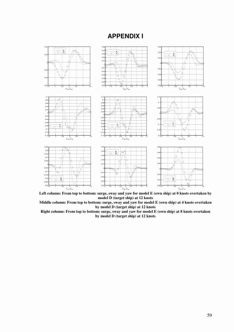
59

APPENDIX I

ξ′s,n

, ξ′s,e

-1.5 -1 -0.5 0 0.5 1 1.5-0.06

-0.04

-0.02

0

0.02

0.04

X′nX′e

ξ′s,n

, ξ′s,e

-2 -1.5 -1 -0.5 0 0.5 1 1.5 2-0.06

-0.05

-0.04

-0.03

-0.02

-0.01

0

0.01

0.02

0.03

0.04

0.05

X′nX′e

ξ′s,n

, ξ′s,e

-1.5 -1 -0.5 0 0.5 1 1.5-0.08

-0.06

-0.04

-0.02

0

0.02

0.04

0.06

X′nX′e

ξ′s,n

, ξ′s,e

-1.5 -1 -0.5 0 0.5 1 1.5-0.14

-0.12

-0.1

-0.08

-0.06

-0.04

-0.02

0

0.02

0.04

0.06

0.08

0.1

Y′n

Y′e

ξ′s,n

, ξ′s,e

-2 -1.5 -1 -0.5 0 0.5 1 1.5 2-0.14

-0.12

-0.1

-0.08

-0.06

-0.04

-0.02

0

0.02

0.04

0.06

0.08

0.1

0.12

Y′nY′e

ξ′s,n

, ξ′s,e

-1.5 -1 -0.5 0 0.5 1 1.5-0.2

-0.15

-0.1

-0.05

0

0.05

0.1

0.15

Y′n

Y′e

ξ′s,n

, ξ′s,e

-1.5 -1 -0.5 0 0.5 1 1.5-0.03

-0.025

-0.02

-0.015

-0.01

-0.005

0

0.005

0.01

0.015

0.02

0.025

N′nN′e

ξ′s,n

, ξ′s,e

-2 -1.5 -1 -0.5 0 0.5 1 1.5 2-0.04

-0.03

-0.02

-0.01

0

0.01

0.02

0.03

0.04

0.05

N′nN′e

ξ′s,n

, ξ′s,e

-1.5 -1 -0.5 0 0.5 1 1.5-0.06

-0.04

-0.02

0

0.02

0.04

0.06

0.08

N′nN′e

Left column: From top to bottom: surge, sway and yaw for model E (own ship) at 0 knots overtaken by

model D (target ship) at 12 knots

Middle column: From top to bottom: surge, sway and yaw for model E (own ship) at 4 knots overtaken

by model D (target ship) at 12 knots

Right column: From top to bottom: surge, sway and yaw for model E (own ship) at 8 knots overtaken

by model D (target ship) at 12 knots

60

APPENDIX II

ξ′s,n

, ξ′s,e

-1.5 -1 -0.5 0 0.5 1 1.5-0.03

-0.02

-0.01

0

0.01

0.02

0.03

0.04

X′nX′e

ξ′s,n

, ξ′s,e

-1.5 -1 -0.5 0 0.5 1 1.5-0.04

-0.03

-0.02

-0.01

0

0.01

0.02

0.03

0.04

X′nX′e

ξ′s,n

, ξ′s,e

-1.5 -1 -0.5 0 0.5 1 1.5-0.025

-0.02

-0.015

-0.01

-0.005

0

0.005

0.01

0.015

0.02

0.025

X′nX′e

ξ′s,n

, ξ′s,e

-1.5 -1 -0.5 0 0.5 1 1.5-0.5

-0.4

-0.3

-0.2

-0.1

0

0.1

0.2

0.3

Y′nY′e

ξ′s,n

, ξ′s,e

-1.5 -1 -0.5 0 0.5 1 1.5-0.4

-0.3

-0.2

-0.1

0

0.1

0.2

Y′nY′e

ξ′s,n

, ξ′s,e

-1.5 -1 -0.5 0 0.5 1 1.5-0.2

-0.15

-0.1

-0.05

0

0.05

0.1

Y′nY′e

ξ′s,n

, ξ′s,e

-1.5 -1 -0.5 0 0.5 1 1.5-0.06

-0.04

-0.02

0

0.02

0.04

0.06

N′nN′e

ξ′s,n

, ξ′s,e

-1.5 -1 -0.5 0 0.5 1 1.5-0.04

-0.02

0

0.02

0.04

0.06

N′nN′e

ξ′s,n

, ξ′s,e

-1.5 -1 -0.5 0 0.5 1 1.5-0.03

-0.025

-0.02

-0.015

-0.01

-0.005

0

0.005

0.01

0.015

0.02

0.025

N′nN′e

From top to bottom: surge, sway and yaw for model E (own ship) at 12 knots encountering model D

(target ship) at 12 knots

Left column: Water depth h = 17.08 metres

Middle column: Water depth h = 18.63 metres

Right column: Water depth h = 23.04 metres