Vacuum I

Giuliano FranchettiGSI Darmstadt, D-64291 Darmstadt, Germany

AbstractThis paper is an introduction to the basics of vacuum. It is intended for readersunfamiliar with the topic; more advanced treatments are left to the dedicatedCERN Accelerator School on vacuum in accelerators and to the specializedliterature. The kinetics of gases, and gas flows through pipes and pumps arereviewed here. The topic of pumps is continued in the paper ‘Vacuum II’.

1 Vacuum, mean free path, and beam lifetime

In accelerators, the beam dynamics has the general purpose of controlling the beam particles. For chargedparticles, this happens through the Lorenz force:

dmγ~v

dt= q ~E + q~v × ~B, (1)

where q is the charge of the particle and m is the mass. The time and space structure of the electric andmagnetic fields ~E and ~B in an accelerator has the purpose of guiding beam particles along the designtrajectory. However, in a particle accelerator there is also present a jungle of unwanted particles, whichcreates a background that is damaging to beam operation and experiments. These particles are referredto as ‘residual gas’. As the particles that make up the ‘vacuum’ are not controlled by an electromagneticfield, they are in general treated as a gas in the thermodynamic sense, which is therefore characterized bymacroscopic quantities such as the pressure P , temperature T , particle density n, and composition. Thestatistical behaviour of vacuum particles is described by kinetic theory [1, 2]. In accelerators, the aim ofall of the vacuum systems is to minimize the interaction of the beam with the residual gas. Table 1 listssome typical values of particle densities for different types of vacuum.

Table 1: Examples of particle densities (from Ref. [3])

Particles m−3

Atmosphere 2.5× 1025

Vacuum cleaner 2× 1025

Freeze-dryer 1022

Light bulb 1020

Thermos flask 1019

TV tube 1014

Low Earth orbit (300 km) 1014

H2 in LHC ∼ 1014

SRS/Diamond 1013

Surface of Moon 1011

Interstellar space 105

One fundamental process in a gas is particle–wall collisions. The velocity of a particle afterinteraction with a wall depends on the particle–wall processes that occur. However, in any case, thesecollisions are responsible for creating the macroscopic pressure. The SI unit of pressure is the pascal,Pa = N/m2. Although this is the standard unit, there are also other units in common use, such as the

Table 2: Classification of types of vacuum

Low vacuum Atmospheric pressure to 1 mbarMedium vacuum 1 to 10−3 mbarHigh vacuum (HV) 10−3 to 10−8 mbarUltrahigh vacuum (UHV) 10−8 to 10−12 mbarExtreme high vacuum (XHV) Less than 10−12 mbar

bar, torr, and atmosphere, which are related to each other by 1 Pa = 10−2 mbar = 7.5 × 10−3 Torr =9.87× 10−6 atm. Table 2 shows the classification of types of vacuum in terms of pressure.

Another important process in a gas is particle–particle collisions. This process is the most prob-able process, as collisions between three or more particles are possible but rather unlikely. In elasticcollisions, two fundamental quantities are preserved: energy and momentum. Particle–particle collisionsare responsible for creating a distribution of velocities in the particles of a gas. The temperature of thegas is related to the mean kinetic energy of a particle: for monatomic particles, 1

2m〈v2〉 = 32kBT , where

kB = 1.38 × 10−23 J·K−1 is the Boltzmann constant. For example, for air, assumed to be composedmainly of nitrogen N2, at T = 20◦C, we find

√

〈v2〉 = 511 m/s. This is not the average velocity va,which is slightly smaller; in fact, va = 〈v〉 = 0.92

√

〈v2〉 = 470 m/s. When the gas is in equilibrium, thevelocity distribution of the molecules follows the Maxwell–Boltzmann distribution

1

N

dN

dv=

4√π

(

m

2kBT

)3/2

v2e−mv2/2kBT . (2)

This distribution is shown in Fig. 1. The most probable velocity is vα =√

2kBT/m, and the averagevelocity is va =

√

(8/π)(kBT/m). As previously discussed, a gas is characterized by its pressure,

v/vα

1N

dNd(v/vα)

vavα

vrvα

1

4√

πe−1

Fig. 1: Maxwell–Boltzmann distribution

temperature, and volume. When the gas is in equilibrium, i.e., in a stationary state, these quantities arerelated by the equation of state PV = nR0T , where R0 = 8.31 N·m/(mole·K). The pressure is measuredin pascals and the volume in m3, n is the number of moles (1 mole contains a number of particles equalto Avogadro’s number NA), R0 = NAkB, and T is the absolute temperature, expressed in kelvin.

In vacuum physics, the concept of the mean free path plays an important role in determining thebehaviour of a gas. Consider a set of particles at rest, and let the particle density of this distribution be n.Now consider N test particles distributed in a plane of area A. If this plane now moves ‘orthogonally’through the remainder of the gas, when the plane is displaced by a distance ∆l, the test particles willhave spanned a volume A×∆l (see Fig. 2). On the other hand, these particles have a cross-section withrespect to the remainder of the gas of σ = πr2, where r is the radius of the cross-section. The particlespresent in the spanned volume will then cover (with respect to interaction with the test particles) the

available area by an amount ∆A = A×∆l nσ. Therefore the number of particles that will pass, withoutcollision, through the portion of gas of length ∆l is N − N(A ×∆l nσ)/A. We obtain the differentialequation

dN

dl= −N × nσ. (3)

By integrating this equation, we find the number of surviving test particles N(l) at a distance l. Thisquantity can be interpreted as the number of particles that did not collide in a distance l, and of theseparticles, certainly N(l) × ∆l nσ will collide with the remaining gas between l and l + ∆l. Thereforethe probability that a particle will travel for a distance l and then collide with the remaining gas in theinterval between l and l + dl is dP (l) = (N(l)/N0)nσ dl, where N0 is the initial number of particles inthe plane considered. The average distance that a test particle will travel between two collisions is thenλ =

∫

∞

0 l dP (l) = 1/σn. Note that in this argument it is assumed that the particles of the gas are at rest,which is not true in a real gas. Maxwell computed the effect of the relative motion of particles of thesame species, and this adds a factor to the formula, which becomes

λ =1√2σn

. (4)

Fig. 2: Conceptual discussion of the mean free path

For example, if we consider air at T = 20◦C and a pressure P = 1 atm, we find from the equationof state that n = P/(kBT ) = 2.47×1025 atoms/m3. The diameter d of an air molecule is 3.74×10−10 m[2], from which σ = πd2 = 4.39 × 10−19 m2. Therefore the mean free path is λ = 6.51 × 10−8 m.Table 3 shows the relation between the mean free path and the pressure and viscosity for N2 at T = 20◦C,taking d = 3.15× 10−10 m (obtained from measurements of viscosity [4]).

In synchrotrons and colliders, the circulating beam is disturbed by the presence of residual gas.The importance of the residual gas is of high relevance for circular accelerators, where the beam cir-culates for a large number of turns. The situation here is of a beam formed by a number of ions of acertain species, which while travelling may collide with residual gas molecules, become ionized, and belost because they now have the wrong charge state with respect to the machine rigidity. The number ofparticles surviving a path of length ∆l is

N(l +∆l) = N(l)−N(l)σn∆l.

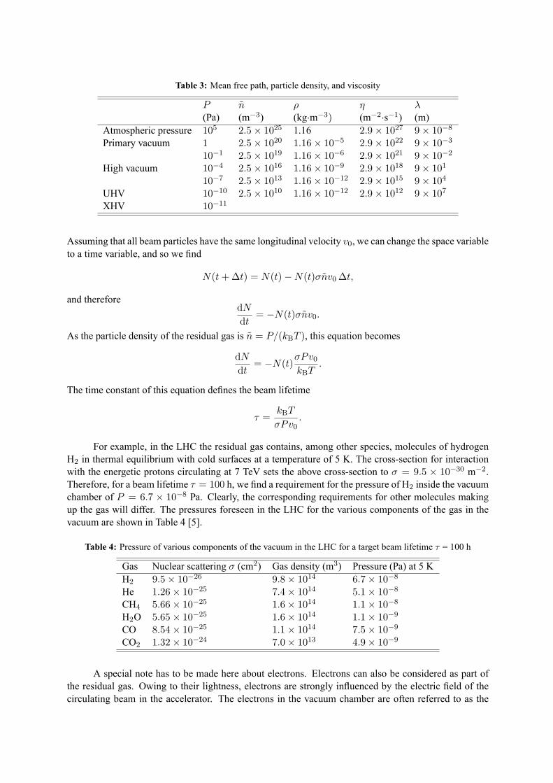
Table 3: Mean free path, particle density, and viscosity

P n ρ η λ(Pa) (m−3) (kg·m−3) (m−2·s−1) (m)

Atmospheric pressure 105 2.5× 1025 1.16 2.9× 1027 9× 10−8

Primary vacuum 1 2.5× 1020 1.16× 10−5 2.9× 1022 9× 10−3

10−1 2.5× 1019 1.16× 10−6 2.9× 1021 9× 10−2

High vacuum 10−4 2.5× 1016 1.16× 10−9 2.9× 1018 9× 101

10−7 2.5× 1013 1.16× 10−12 2.9× 1015 9× 104

UHV 10−10 2.5× 1010 1.16× 10−12 2.9× 1012 9× 107

XHV 10−11

Assuming that all beam particles have the same longitudinal velocity v0, we can change the space variableto a time variable, and so we find

N(t+∆t) = N(t)−N(t)σnv0∆t,

and thereforedN

dt= −N(t)σnv0.

As the particle density of the residual gas is n = P/(kBT ), this equation becomes

dN

dt= −N(t)

σPv0kBT

.

The time constant of this equation defines the beam lifetime

τ =kBT

σPv0.

For example, in the LHC the residual gas contains, among other species, molecules of hydrogenH2 in thermal equilibrium with cold surfaces at a temperature of 5 K. The cross-section for interactionwith the energetic protons circulating at 7 TeV sets the above cross-section to σ = 9.5 × 10−30 m−2.Therefore, for a beam lifetime τ = 100 h, we find a requirement for the pressure of H2 inside the vacuumchamber of P = 6.7 × 10−8 Pa. Clearly, the corresponding requirements for other molecules makingup the gas will differ. The pressures foreseen in the LHC for the various components of the gas in thevacuum are shown in Table 4 [5].

Table 4: Pressure of various components of the vacuum in the LHC for a target beam lifetime τ = 100 h

Gas Nuclear scattering σ (cm2) Gas density (m3) Pressure (Pa) at 5 KH2 9.5× 10−26 9.8× 1014 6.7× 10−8

He 1.26× 10−25 7.4× 1014 5.1× 10−8

CH4 5.66× 10−25 1.6× 1014 1.1× 10−8

H2O 5.65× 10−25 1.6× 1014 1.1× 10−9

CO 8.54× 10−25 1.1× 1014 7.5× 10−9

CO2 1.32× 10−24 7.0× 1013 4.9× 10−9

A special note has to be made here about electrons. Electrons can also be considered as part ofthe residual gas. Owing to their lightness, electrons are strongly influenced by the electric field of thecirculating beam in the accelerator. The electrons in the vacuum chamber are often referred to as the

‘electron cloud’. Reviews of the complex processes of build-up of electrons and their interplay with thecirculating bunches can be found in Refs. [6, 7, 8].

As previously mentioned, the molecules of the vacuum are subject to collisions with one another,generating a Maxwellian distribution of velocities. One relevant feature of a gas is the ‘impingementrate’ J . This quantity measures the number of molecules that hit a unit area of a surface per unit of time.For a Maxwell–Boltzmann velocity distribution, we find [9, 2]

J =1

4nva,

where va =√

(8/π)(kBT/m) is the average velocity of a gas molecule.

2 Gas flows in pipes

The properties of a gas with respect to transport through pipes depend very much on the spatial scaleconsidered, which is set by the size of the pipe or vessel. If the size D of the vessel is much larger thanthe mean free path λ, then the gas will be dominated by collisions between the gas molecules, and theeffect of molecule–wall collisions will be negligible. In this regime, the gas will effectively behave as acontinuum, as a local change in properties will be propagated as a wave (like sound in air at atmosphericpressure and room temperature). If instead the size of the vessel is much smaller than the mean free path,the molecules will collide mainly with the walls of the vessel. In this case continuum processes are notpossible, and the motion of the particles of the gas is dominated by particle–wall collisions. This regimeis referred to as the ‘molecular regime’. The Knudsen number Kn characterizes the type of regime inwhich a gas is found:

Kn = λD

Kn < 0.01 Continuous regime,

0.01 < Kn < 0.5 Transitional regime,

Kn > 0.5 Molecular regime.

2.1 Throughput and conductances

The creation of a vacuum requires the extraction of air from a vessel, which is done via a system ofpumps connected to vessels through pipes.

We now present a short discussion of gas flow in pipes. The flow of a gas through a pipe canbe expressed in terms of the number of particles per second dN/dt passing through a reference surfaceacross the pipe. On the other hand, measurements of gas flow are better expressed in terms of macro-scopic quantities characterizing the thermodynamic state of the gas. If a gas flows in a pipe at a velocityv across an area A, the rate of particles per second dN/dt is

dN

dt= nvA =

P

kBTvA =

P

kBT

dV

dt=

1

kBT

d

dtPV. (5)

Note that the quantity Q = PV here is a product of a pressure and a volume. Equation (5) can bere-expressed so that the particle flow is

dN

dt=

1

kBTQ.

The quantity Q is called the throughput and is expressed in Pa·m3/s. In the absence of adsorption ordesorption, the rate at which particles pass through a cross-section of a pipe does not change along thepipe, and hence the throughput does not change either.

It is now useful to introduce the concept of the conductance of a pipe. If there is a flow of particlesin a pipe from a section 1 with pressure P1 to a section 2 with pressure P2 (< P1), the relation between

the throughput and the difference in pressure between the two sections can be expressed as

C =Q

P1 − P2. (6)

Here C is the conductance; this is a geometric property of the pipe and of the gas flow. The unitsof C are m3/s. For a composite structure formed from several pipes, it is possible to prove, basedon the assumption that the throughput is conserved, that for N pipes each having conductance Ci, theconductance C of the composition in series is given by

1

C=

N∑

i=1

1

Ci.

For the composition of pipes in parallel, the conductance of the composite structure is

C =N∑

i=1

Ci.

Note that the law of composition of pipes in series can be used to obtain an indication of howthe conductance of a long pipe scales with the length. In fact, if C1 is the conductance of one pipe, byconnecting N of these pipes in series we find a conductance C = C1/N . Therefore it is expected thatthe conductance scales as the inverse of the length of the pipe.

Up to this point, the concept of conductance, alias the relation between the throughput and thepressure gradient, has been discussed without considering the physical behaviour of the gas itself. It istherefore to be expected that a pipe will exhibit different conduction properties according to whether thegas is in a molecular or a continuum regime.

2.2 Molecular flow

Particle–wall collisions characterize the molecular flow of a gas in a pipe. For example, in a vessel ofdiameter D = 0.1 m, the molecular regime Kn > 0.5 is obtained for a pressure of P < 1.3×10−3 mbar(at room temperature).

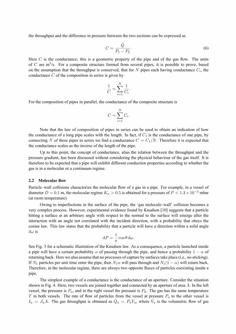
Owing to imperfections in the surface of the pipe, the ‘gas molecule–wall’ collision becomes avery complex process. However, experimental evidence found by Knudsen [10] suggests that a particlehitting a surface at an arbitrary angle with respect to the normal to the surface will emerge after theinteraction with an angle not correlated with the incident direction, with a probability that obeys thecosine law. This law states that the probability that a particle will have a direction within a solid angledω is

dP =1

πcos θ dω.

See Fig. 3 for a schematic illustration of the Knudsen law. As a consequence, a particle launched insidea pipe will have a certain probability α of passing through the pipe, and hence a probability 1 − α ofreturning back. Here we also assume that no processes of capture by surfaces take place (i.e., no sticking).If N1 particles per unit time enter the pipe, then N1α will pass through and N1(1− α) will return back.Therefore, in the molecular regime, there are always two opposite fluxes of particles coexisting inside apipe.

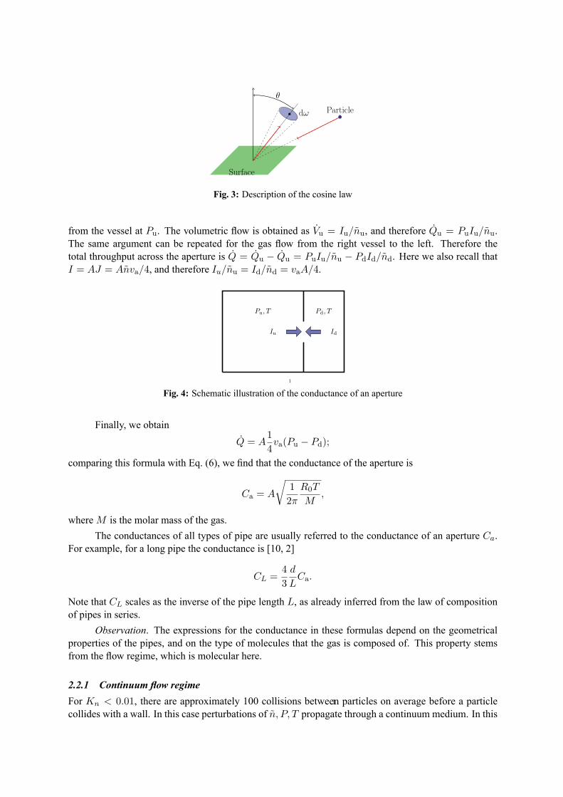
The simplest example of a conductance is the conductance of an aperture. Consider the situationshown in Fig. 4. Here, two vessels are joined together and connected by an aperture of area A. In the leftvessel, the pressure is Pu, and in the right vessel the pressure is Pd. The gas has the same temperatureT in both vessels. The rate of flow of particles from the vessel at pressure Pu to the other vessel isIu = JuA. The gas throughput is obtained as Qu = PuVu, where Vu is the volumetric flow of gas

θ

dω

Surface

Particle

1

Fig. 3: Description of the cosine law

from the vessel at Pu. The volumetric flow is obtained as Vu = Iu/nu, and therefore Qu = PuIu/nu.The same argument can be repeated for the gas flow from the right vessel to the left. Therefore thetotal throughput across the aperture is Q = Qu − Qu = PuIu/nu − PdId/nd. Here we also recall thatI = AJ = Anva/4, and therefore Iu/nu = Id/nd = vaA/4.

Iu Id

Pu, T Pd, T

1

Fig. 4: Schematic illustration of the conductance of an aperture

Finally, we obtain

Q = A1

4va(Pu − Pd);

comparing this formula with Eq. (6), we find that the conductance of the aperture is

Ca = A

√

1

2π

R0T

M,

where M is the molar mass of the gas.

The conductances of all types of pipe are usually referred to the conductance of an aperture Ca.For example, for a long pipe the conductance is [10, 2]

CL =4

3

d

LCa.

Note that CL scales as the inverse of the pipe length L, as already inferred from the law of compositionof pipes in series.

Observation. The expressions for the conductance in these formulas depend on the geometricalproperties of the pipes, and on the type of molecules that the gas is composed of. This property stemsfrom the flow regime, which is molecular here.

2.2.1 Continuum flow regime

For Kn < 0.01, there are approximately 100 collisions between particles on average before a particlecollides with a wall. In this case perturbations of n, P, T propagate through a continuum medium. In this

regime, collisions between particles create the phenomenon of viscosity, which affects the behaviour ofgases in pipes.

If a fluid propagates into a pipe at a ‘small’ speed, the fluid is in the laminar regime and the motionof the particles is parallel to the pipe axis (see Ref. [11] for extensive discussions of flow in pipes). Thevelocity of the fluid is zero at the walls of the pipe, and is largest at the centre. If the velocity of the fluidis increased beyond a certain threshold, the fluid changes its properties and its motion becomes turbulent.The quantity that defines the transition from the viscous laminar regime to the turbulent regime is theReynolds number

Re =ρvDh

η,

where ρ is the density of the fluid in kg/m3, v is the average velocity of the gas in m/s, and Dh is thehydraulic diameter in metres, given by Dh = 4A/B, where A is the cross-sectional area and B is theperimeter of the pipe. Finally, η is the viscosity in Pa·s. If Re < 2000, the fluid is in the laminar regime,whereas for Re > 3000 the fluid is in the turbulent regime.

The Reynolds number can be expressed in terms of the throughput as

Re = 4Q

B

M

R0T

1

η.

For air (N2) at T = 20◦C, taking η = 1.75 × 10−5 Pa·s, we find Re = kRQ/B, where kR =2.615 s/(m2·Pa). Therefore the transition to turbulent flow (Re ∼ 2000) takes place at a transitionthroughput QT = 24d, where QT is in mbar·l/s. For a pipe of diameter d = 25 mm, we obtainQT = 600 mbar·l/s, which corresponds at atmospheric pressure to a speed of v = 1.22 m/s.

2.2.1.1 Laminar regime

One source of complexity in characterizing a fluid flow in a pipe is the compressibility of the fluid.However, it is possible to prove that if the velocity of the fluid has a Mach number Ma < 0.2, then a fluidin a pipe behaves as if it were incompressible, i.e., the Bernoulli equation takes a form very similar tothat of the equation for incompressible fluids.

It is important to characterize pipes in terms of the conductance when the flow regime is laminar.The conductance can be given under some assumptions about the laminar flow: (1) the fluid is consideredincompressible; (2) the flow is fully developed, that is, it reaches a velocity distribution which does notchange along a pipe of constant cross-section (see [2] for further discussion); (3) the particle motion islaminar (Re < 2000); and (4) the velocity of the fluid at the pipe walls is zero. Under these assumptions,we find that the throughput is given by Q = C(Pu − Pd), where the conductance is now given by

C =πD4

128ηLP ,

where P = (Pu + Pd)/2. Here Pu is the pressure upstream, Pd is the pressure downstream, D is thediameter of the pipe, L is its length, and η is the fluid viscosity. This finding can be obtained directly fromthe Hagen–Poiseuille equation [11]. We conclude that in a continuum laminar regime, the conductancedepends on the pressure at which the fluid transport occurs.

2.2.1.2 Turbulent regime

In the turbulent regime, for a long pipe, the expression for the throughput becomes

Q = A

√

R0T

M

√

Dh

fDL

√

P 2u − P 2

d ,

where fD is the Darcy friction factor, a quantity which depends nonlinearly on the Reynolds number[12].

3 Sources of vacuum degradation

After the air has been pumped out from a chamber, the vacuum can degrade because new molecules mayenter the vessel.

One phenomenon that contributes to spoiling the vacuum is the evaporation and condensation ofliquids present on surfaces (because those surfaces have not been cleaned). If there is a spot of liquidon a surface in a high-vacuum vessel, particles evaporate from the surface of the liquid, increasing thepressure in the vessel. At the same time, vapour particles in the vessel impinge on the liquid surface,bringing molecules into the liquid. There are therefore two fluxes of particles: one of evaporation and theother of condensation. The process of condensation depends on the pressure in the vessel, whereas theevaporation process depends only on the temperature. If one waits long enough, the pressure in the vesselwill stabilize to the saturated vapour pressure PE, the value of which is given by the Clausius–Clapeyronequation [13]. Therefore we conclude that the fluxes of evaporation JE and condensation JC are equal.Hence the evaporation flux is

JE = PENa1√

2πR0MT.

A spot of liquid in a vacuum chamber will therefore emit a flux of particles JE. This is equivalent to athroughput into the vessel equal to QE = AJEkBT , where A is the surface area of liquid exposed to thevacuum in the vessel.

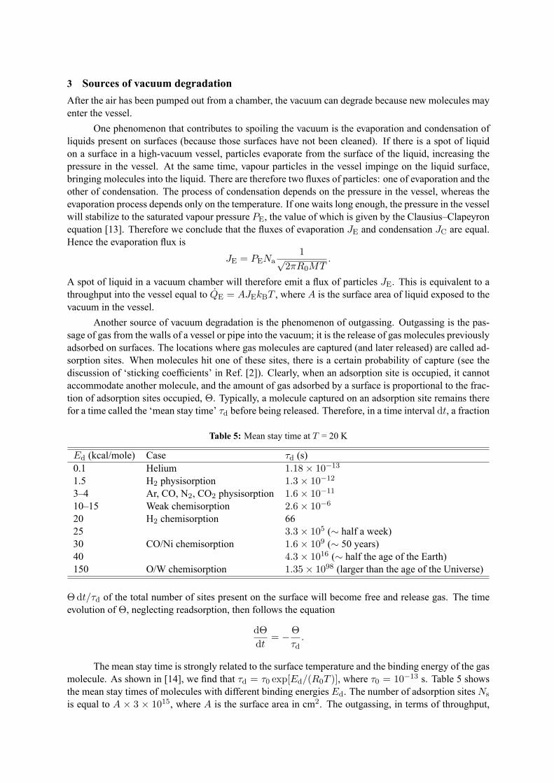
Another source of vacuum degradation is the phenomenon of outgassing. Outgassing is the pas-sage of gas from the walls of a vessel or pipe into the vacuum; it is the release of gas molecules previouslyadsorbed on surfaces. The locations where gas molecules are captured (and later released) are called ad-sorption sites. When molecules hit one of these sites, there is a certain probability of capture (see thediscussion of ‘sticking coefficients’ in Ref. [2]). Clearly, when an adsorption site is occupied, it cannotaccommodate another molecule, and the amount of gas adsorbed by a surface is proportional to the frac-tion of adsorption sites occupied, Θ. Typically, a molecule captured on an adsorption site remains therefor a time called the ‘mean stay time’ τd before being released. Therefore, in a time interval dt, a fraction

Table 5: Mean stay time at T = 20 K

Ed (kcal/mole) Case τd (s)0.1 Helium 1.18× 10−13

1.5 H2 physisorption 1.3× 10−12

3–4 Ar, CO, N2, CO2 physisorption 1.6× 10−11

10–15 Weak chemisorption 2.6× 10−6

20 H2 chemisorption 6625 3.3× 105 (∼ half a week)30 CO/Ni chemisorption 1.6× 109 (∼ 50 years)40 4.3× 1016 (∼ half the age of the Earth)150 O/W chemisorption 1.35× 1098 (larger than the age of the Universe)

Θdt/τd of the total number of sites present on the surface will become free and release gas. The timeevolution of Θ, neglecting readsorption, then follows the equation

dΘ

dt= −Θ

τd.

The mean stay time is strongly related to the surface temperature and the binding energy of the gasmolecule. As shown in [14], we find that τd = τ0 exp[Ed/(R0T )], where τ0 = 10−13 s. Table 5 showsthe mean stay times of molecules with different binding energies Ed. The number of adsorption sites Ns

is equal to A × 3 × 1015, where A is the surface area in cm2. The outgassing, in terms of throughput,

then becomes

QG = kBTNsΘ

τd.

A third source of vacuum degradation is the presence of leaks. If a small hole (i.e., a smallchannel) is created in a vessel containing a high vacuum, then the throughput of gas from the outsideto the inside of the vessel is given by Q ≃ CaP0, where P0 is the atmospheric pressure (or, moregenerally, the outside pressure). In the case of air, composed mainly of N2, at room temperature T =293 K, for a small hole of diameter d = 10−10 m we find a conductance Ca = 9.17 × 10−19 m3/s.Therefore the throughput is QL = 9.17 × 10−14 Pa·m3/s = 9.17 × 10−13 mbar·l/s. For a hole withd = 10−9 m, QL ≃ 10−10 mbar·l/s, and therefore 1 cm3 of air needs 317 years to enter the vessel.Leaks in a vacuum system can be distinguished into the following classes according to the throughput[15]: ‘very tight’ if QL < 10−6 mbar·l/s, ‘tight’ if 10−6 < QL < 10−5 mbar·l/s, and ‘with leaks’ if10−5 < QL < 10−4 mbar·l/s.

Finally, among the sources of vacuum degradation, we should mention the phenomenon of per-meation: this process happens when gases are adsorbed on the material of the walls, diffuse through thewalls, and are later desorbed into the vessel. The throughput depends on the surface temperature, thethickness and composition of the walls, and the composition of the gas. A discussion of this effect hasbeen given in Ref. [2].

4 Pipes and pumps

The creation of a vacuum is achieved via pumps that are connected to vessels via pipes. An ideal pumpbehaves in such a way that all of the gas particles that enter the pump inlet never return. The pumpingspeed of a pump is referred to the volumetric speed S of the gas through the inlet, and is expressed inunits of m3/s. If the inlet of a pump has diameter D, then the gas flow through the ideal pump apertureis given by I = JD2π/4, where I is the number of molecules per second passing through the inletsurface. The volumetric pumping speed is then S = dV/dt = I/n = vaD

2π/16. For example, for N2

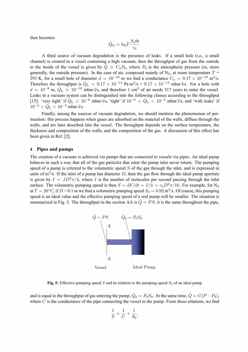
at T = 20◦C, if D = 0.1 m we find a volumetric pumping speed S0 = 0.92 m3/s. Of course, this pumpingspeed is an ideal value and the effective pumping speed of a real pump will be smaller. The situation issummarized in Fig. 5. The throughput in the section AA is Q = PS; it is the same throughout the pipe,

Q = PS Q0 = P0S0

Vessel Ideal Pump

A

A

Fig. 5: Effective pumping speed S and its relation to the pumping speed S0 of an ideal pump

and is equal to the throughput of gas entering the pump, Q0 = P0S0. At the same time, Q = C(P −P0),where C is the conductance of the pipe connecting the vessel to the pump. From these relations, we find

1

S=

1

C+

1

S0,

which gives the effective pumping speed of an ideal pump. For example, taking a long pipe, CL =4D/(3L)Ca, and noting that the volumetric speed of the ideal pump is S0 = Ca, we find

S =S0

1 + 3L/(4D).

Therefore pumps should be placed as close as possible to vessels in order to exploit the nominal pumpingcapability of the pump.

5 Making the vacuum: pump-down time and ultimate pressure

We now put together all the different sources of vacuum degradation, which are summarized in Fig. 6.The quantity of gas inside a vessel Q varies according to

P, V

S0S

QS

C

QG

QL

QE

Hole

Pump

Fig. 6: Summary of sources of vacuum degradation

Q = QT − QS ,

where QS is the throughput removed by the pump, and QT is the total throughput entering the vesselbecause of sources of vacuum degradation. This equation becomes

dP

dtV = QT − QS , (7)

where V is the volume of the vessel. If the sources of vacuum degradation and the pumping speed areindependent of the pressure in the vessel, the evolution of the pressure, i.e., the solution of Eq. (7), is

P = Pu + (P0 − Pu)e−(S/V )t,

where P0 is the initial pressure at t = 0, and Pu = QT/S. The time constant of the process τpd = V/Sis the pump-down time. From this equation, we see that for t → ∞ the pressure in the vessel convergesto Pu, which is called the ultimate pressure. This pressure is determined by the equilibrium between thethroughput of the sources of degradation and the throughput removed by the pump.

The vacuum requirements vary from project to project. Table 6 lists examples of the vacuumrequirements in the SNS, LHC, and FAIR [16, 5, 17].

6 Pumps

The control and creation of a vacuum is performed via a system of pumps. Pumps are classified accordingto their principle of operation.

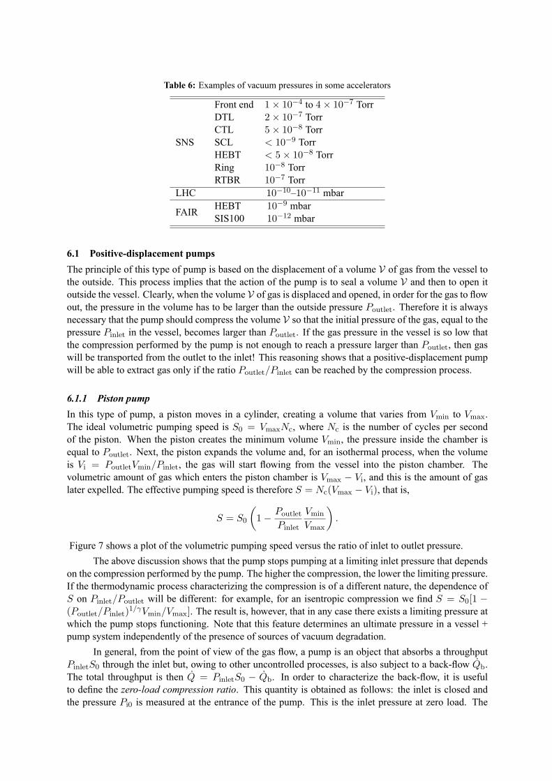
Table 6: Examples of vacuum pressures in some accelerators

SNS

Front end 1× 10−4 to 4× 10−7 TorrDTL 2× 10−7 TorrCTL 5× 10−8 TorrSCL < 10−9 TorrHEBT < 5× 10−8 TorrRing 10−8 TorrRTBR 10−7 Torr

LHC 10−10–10−11 mbar

FAIRHEBT 10−9 mbarSIS100 10−12 mbar

6.1 Positive-displacement pumps

The principle of this type of pump is based on the displacement of a volume V of gas from the vessel tothe outside. This process implies that the action of the pump is to seal a volume V and then to open itoutside the vessel. Clearly, when the volume V of gas is displaced and opened, in order for the gas to flowout, the pressure in the volume has to be larger than the outside pressure Poutlet. Therefore it is alwaysnecessary that the pump should compress the volume V so that the initial pressure of the gas, equal to thepressure Pinlet in the vessel, becomes larger than Poutlet. If the gas pressure in the vessel is so low thatthe compression performed by the pump is not enough to reach a pressure larger than Poutlet, then gaswill be transported from the outlet to the inlet! This reasoning shows that a positive-displacement pumpwill be able to extract gas only if the ratio Poutlet/Pinlet can be reached by the compression process.

6.1.1 Piston pump

In this type of pump, a piston moves in a cylinder, creating a volume that varies from Vmin to Vmax.The ideal volumetric pumping speed is S0 = VmaxNc, where Nc is the number of cycles per secondof the piston. When the piston creates the minimum volume Vmin, the pressure inside the chamber isequal to Poutlet. Next, the piston expands the volume and, for an isothermal process, when the volumeis Vi = PoutletVmin/Pinlet, the gas will start flowing from the vessel into the piston chamber. Thevolumetric amount of gas which enters the piston chamber is Vmax − Vi, and this is the amount of gaslater expelled. The effective pumping speed is therefore S = Nc(Vmax − Vi), that is,

S = S0

(

1− Poutlet

Pinlet

Vmin

Vmax

)

.

Figure 7 shows a plot of the volumetric pumping speed versus the ratio of inlet to outlet pressure.

The above discussion shows that the pump stops pumping at a limiting inlet pressure that dependson the compression performed by the pump. The higher the compression, the lower the limiting pressure.If the thermodynamic process characterizing the compression is of a different nature, the dependence ofS on Pinlet/Poutlet will be different: for example, for an isentropic compression we find S = S0[1 −(Poutlet/Pinlet)

1/γVmin/Vmax]. The result is, however, that in any case there exists a limiting pressure atwhich the pump stops functioning. Note that this feature determines an ultimate pressure in a vessel +pump system independently of the presence of sources of vacuum degradation.

In general, from the point of view of the gas flow, a pump is an object that absorbs a throughputPinletS0 through the inlet but, owing to other uncontrolled processes, is also subject to a back-flow Qb.The total throughput is then Q = PinletS0 − Qb. In order to characterize the back-flow, it is usefulto define the zero-load compression ratio. This quantity is obtained as follows: the inlet is closed andthe pressure Pi0 is measured at the entrance of the pump. This is the inlet pressure at zero load. The

S/S0

Pinlet

Poutlet

1

Vmin

Vmax

1

1− Vmin

Vmax

Fig. 7: Pumping speed of a piston pump

zero-load compression ratio is therefore defined as K0 = P0/Pi0, which is a quantity measurable as afunction of the outlet pressure P0 and the pumping speed. As the throughput at the inlet Q is zero in thisspecial case, we find that the back-flow throughput Qb is equal to S0P0/K0.

For technical reasons, the compression ratio of a pump cannot be made arbitrarily large. Henceother techniques have been developed to improve the lower limit on pressure.

6.1.2 Rotary pumps

These pumps are characterized by a pumping speed S = 1–1500 m3/h. The lowest pressure achievablereaches 5 × 10−2 mbar for one-stage pumps, and 10−3 mbar for two-stage pumps. An illustrationof this type of pump is shown in Fig. 8. These pumps perform the compression via the rotation of

Fig. 8: Illustration of a rotary pump

a rotor, which moves a vane that compresses the gas to a high compression ratio. However, during thecompression, there may be a component G of the gas for which the partial pressure PG becomes too high,resulting in condensation of that component. This problem is avoided by injecting a non-condensablegas during the compression phase. By doing so, the maximum partial pressure PG can be lowered belowthe condensation point. This process is called gas ballast [18].

6.1.3 Liquid-ring pumps

Liquid-ring pumps contain a rotating impeller, the axis of which is off centre relative to the casing (seethe illustration in Fig. 9). Centrifugal force pushes the liquid against the casing, creating a liquid ring,which seals the impeller, creating vanes that enclose a variable volume. The typical pumping speed is1–27 000 m3/h, and gas can be pumped at pressures from 1000 mbar to 33 mbar.

Fig. 9: Illustration of a liquid-ring pump

A problem related to this type of pump arises when the gas expands in the cavities and the pressurebecomes lower than the vapour pressure Ps of the liquid (typically water). At that point the liquid boils,but the motion of the impeller then compresses the gas, causing the vapour bubbles to implode, creatingshock waves in the liquid medium. This phenomenon is called cavitation, and it causes anomalousfunctioning of the pump, setting a limit on the pressure at which the pump can work. At T = 15◦C, thevapour pressure of water is 33 mbar, which is a typical limiting pressure for this type of pump becauseof the need to avoid cavitation. For a review of liquid-ring pumps, see Ref. [19].

6.1.4 Dry vacuum pumps: the Roots pump

These pumps contain two rotating elements which are separated from the case and from each other byapproximately 1 mm. The elements rotate in opposite directions, and as a result of their motion theycreate a moving vane, which brings a gas volume from the inlet to the outlet. The pumping speed is75–30 000 m3/h and the operating pressure is 10–10−3 mbar. An illustration of this type of pump isshown in Fig. 10. For a general reference, see Ref. [20].

Fig. 10: Illustration of a Roots pump

7 Kinetic vacuum pumps

A different class of pumps, based on a different principle, is that of kinetic vacuum pumps. These pumpsgive a momentum to gas particles so that they are moved from the inlet to the outlet.

7.1 Molecular-drag pump

This pump is based on the molecular-drag effect. If a gas molecule hits a surface, it will emerge from itin some direction with a probability determined by the cosine law. However, if the surface is in motionwith a tangential velocity, the molecule will emerge from reflection from the moving surface with anadditional velocity component equal to the speed of the surface. This effect is called the drag effect,and it can be used to create a pump [21]. Consider an long, open channel of transverse cross-sectionh× w closed by a surface moving with a velocity U (Fig. 11 (top)). A gas molecule hitting the moving

Fig. 11: Principle of the drag pump (top), and schematic illustration of gas flow in the channel of a drag pump(bottom)

surface will acquire a velocity U owing to the drag effect. When the molecule hits any of the otherwalls of the channel, it will be reflected on average orthogonally to that surface, by the cosine law (seeFig. 11 (bottom)). Therefore a volumetric flow S0 = whU/2 into the channel is established. Taking theback-flow into account, the pumping speed at the inlet is

Si = S0K −K0

1−K0,

where K0 = Poutlet/Pinlet,0 is the zero-load compression ratio, and K = Poutlet/Pinlet. It can be shownthat the compression ratio at zero load takes the form K0 = exp(S0/C), where C is the conductanceof the channel. For a long tube, S0/C = 3UL/(4hva), where va is the average thermal velocity and Lis the length of the channel. For example, for L = 250 mm and h = 3 mm, we have S0/C > 10 andK0 ≫ 1, so that we retrieve the form

S = S0

(

1− K

K0

)

.

An illustration of the functioning of a molecular-drag pump is shown in Fig. 12. The typicalpumping speed of a molecular-drag pump is 7–300 l/s, at an operating pressure of 10−3–103 Pa. Theultimate pressure reachable is 10−5–10−3 Pa. For references, see Refs. [9, 22].

7.2 Turbomolecular pump

The turbomolecular pump is based on the rotation of a set of blades at a velocity U . The blades are tiltedat an angle φ. The gas molecules enter the inlet, and the motion of the blades imparts a momentum to

Fig. 12: Illustration of the functioning of a molecular-drag pump

the gas. The situation is illustrated in Fig. 13. When particles leave the set of rotating blades, the gashas acquired a rotational velocity, which makes it difficult to use a subsequent series of rotating blades(as they would move at a similar velocity to the gas). For this reason, a stator consisting of blades at restis placed after the rotating blades so as to remove the rotational component of the particle velocity. Byusing this strategy, several rotor + stator blocks can be arranged in a multistage pumping structure.

Fig. 13: Principle of the turbomolecular pump

The probability that molecules entering the pump will be pushed out is W = N/(JiA), where Jiis the rate of impingement of molecules on the inlet surface. The maximum probability Wmax is foundwhen Poutlet = Pinlet. Analogously to the case of the molecular-drag pump, the pumping probability Wis given by

W = WmaxK0 −K

K0 − 1,

where K0 is the compression at zero load. In Ref. [23, 9], it is shown that K0 ∝ g(φ) exp(U/va), and

therefore K0 ∝ exp(√M), where M is the molar mass of the gas. This means that different gas species

have different pumping probabilities. In addition, the maximum probability Wmax is proportional toU/va ∝

√M . Therefore the maximum pumping speed Smax = WmaxJ is independent of the molecular

mass of the gas, andS

Smax=

K0 −K

K0 − 1.

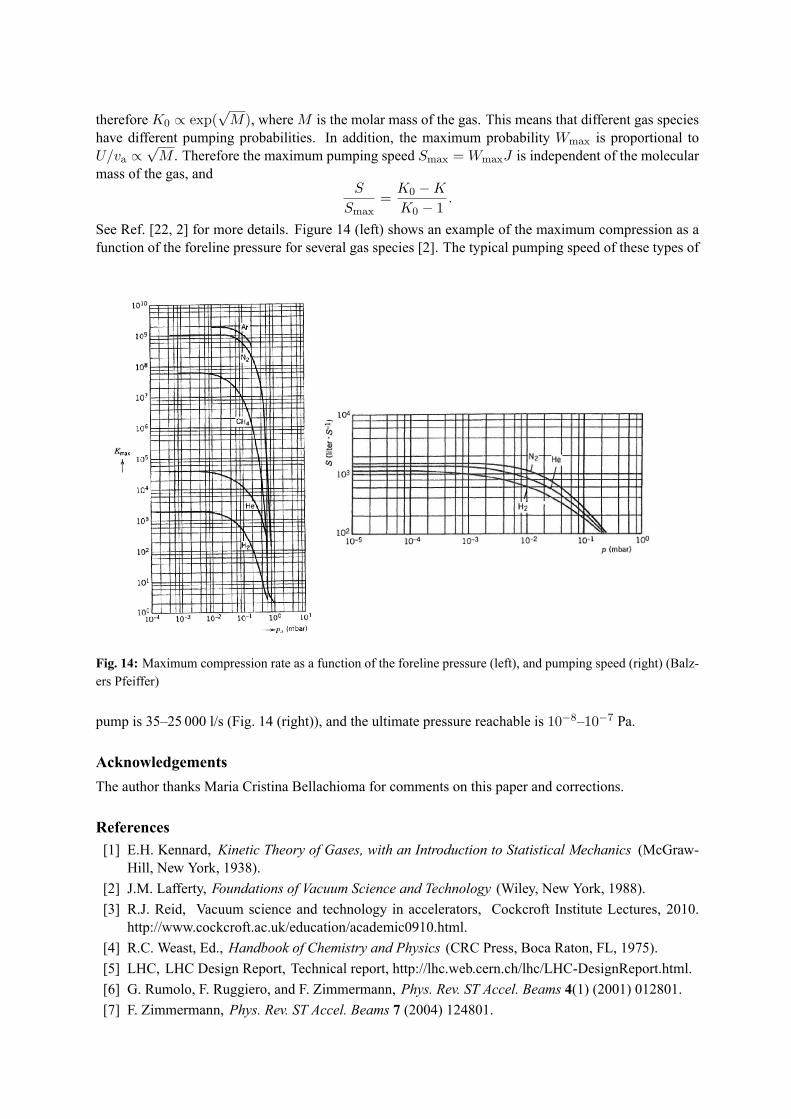
See Ref. [22, 2] for more details. Figure 14 (left) shows an example of the maximum compression as afunction of the foreline pressure for several gas species [2]. The typical pumping speed of these types of

Fig. 14: Maximum compression rate as a function of the foreline pressure (left), and pumping speed (right) (Balz-ers Pfeiffer)

pump is 35–25 000 l/s (Fig. 14 (right)), and the ultimate pressure reachable is 10−8–10−7 Pa.

Acknowledgements

The author thanks Maria Cristina Bellachioma for comments on this paper and corrections.

References[1] E.H. Kennard, Kinetic Theory of Gases, with an Introduction to Statistical Mechanics (McGraw-

Hill, New York, 1938).

[2] J.M. Lafferty, Foundations of Vacuum Science and Technology (Wiley, New York, 1988).

[3] R.J. Reid, Vacuum science and technology in accelerators, Cockcroft Institute Lectures, 2010.http://www.cockcroft.ac.uk/education/academic0910.html.

[4] R.C. Weast, Ed., Handbook of Chemistry and Physics (CRC Press, Boca Raton, FL, 1975).

[5] LHC, LHC Design Report, Technical report, http://lhc.web.cern.ch/lhc/LHC-DesignReport.html.

[6] G. Rumolo, F. Ruggiero, and F. Zimmermann, Phys. Rev. ST Accel. Beams 4(1) (2001) 012801.

[7] F. Zimmermann, Phys. Rev. ST Accel. Beams 7 (2004) 124801.

[8] M.A. Furman and M.T.F. Pivi, Phys. Rev. ST Accel. Beams 5 (2002) 124404.

[9] A. Chambers, Modern Vacuum Physics (CRC Press, Boca Raton, FL, 2004).

[10] M. Knudsen, Ann. Phys. 28 (1909) 75.

[11] R.B. Bird, W.E. Stewart, and E.N. Lightfoot, Transport Phenomena (Wiley, New York, 2007).

[12] S.E. Haaland, J. Fluids Eng. 105 (1983) 89.

[13] C.H. Collie, Kinetic Theory and Entropy (Longman, London, 1982).

[14] P.A. Redhead, J. Vac. Sci. Technol. A 13 (1995) 2791.

[15] K. Zapfe, Leak detection, CERN Accelerator School, CERN-2007-003 (2007), p. 227.

[16] J.Y. Tang, SNS vacuum instrumentation and control system, Proc. 8th International Conf. onAccelerator and Large Experimental Physics Control Systems, San Jose, CA, 2001, p. 188.

[17] A. Kraemer, The vacuum system of FAIR accelerator facility, Proc. EPAC 2006, Edinburgh, 2006,p. 1429.

[18] W. Gaede, Z. Naturforsch. 2a (1947) 233–238.

[19] H. Bannwarth, Liquid Ring Vacuum Pumps, Compressors and Systems (Wiley-VCH, Weinheim,2005).

[20] A.P. Troup and N.T.M. Dennis, J. Vac. Sci. Technol. A 9 (1991) 2048.

[21] W. Gaede, Ann. Phys. 346(7) (1913) 337–380.

[22] J.F. O’Hanlon, A User’s Guide to Vacuum Technology (Wiley, Hoboken, NJ, 2003).

[23] C.H. Kruger and A.H. Shapiro, in Rarefied Gas Dynamics, Ed. L. Talbot (Academic Press, NewYork, 1960), p. 117.