Two types of flow can be distinguished in gas-liquid flows in bubble columns: bubbly flowand churn-turbulent flow. The bubbly flowregime is characterized by uniform flow ofbubbles of uniform size. Churn-turbulent flow,on the other hand, is characterized by a widevariation in bubble sizes with large bubblesrising rapidly and causing liquid circulation.

Flotation columns are normally operated inthe bubbly flow regime, which is the optimalcondition for column flotation (Finch andDobby, 1990; Yianatos and Finch, 1990;Ityokumbul, 1992). However, it has beengenerally observed that flotation columnperformance deteriorates when the superficialgas velocity is increased beyond a certain limitwhere the flow regime changes from bubblyflow to churn-turbulent flow (Xu, Finch, and

Uribe-Salas, 1991). The identification of thiscritical or maximum superficial gas velocity istherefore important for optimal operation offlotation columns.

Xu, Finch, and Uribe-Salas (1991) and Xuet al. (1989) investigated three phenomenathat can be used to identify the maximumsuperficial gas velocity in column flotation:loss of interface, loss of positive bias flow, andloss of bubbly flow. Loss of interface occurswhen the hydrodynamic conditions in the frothzone of the column become identical to theconditions prevailing in the collection zone.This will result in the loss of the cleaningaction associated with the froth zone.

In column flotation, wash water, which iscontinuously added at the top of the column,maintains a net downward flow of water thatprevents entrained particles from reaching theconcentrate. This net downward flow of wateris referred to as positive bias flow. Byminimizing entrainment of unwanted particles,a positive bias maximizes the concentrategrade. Loss of positive bias occurs when thesuperficial gas velocity is high enough to causea reversal of the net flow of water at thefroth/collection zone interface.

On the other hand, the loss of bubbly flowoccurs when the superficial gas velocity issufficiently high to bring about a transitionfrom bubbly flow conditions to churn-turbulent flow. The increased mixingassociated with churn-turbulent flow isunfavourable for mineral recovery in thecolumn.

Considering the froth and liquid (pulp)phases as distinct flow regimes with differentliquid holdups, Langberg and Jameson (1992)investigated the hydrodynamic conditionsunder which the froth and pulp phases can

Investigation of flow regime transitionin a column flotation cell using CFDby I. Mwandawande*, G. Akdogan*, S.M. Bradshaw*, M. Karimi†, and N. Snyders*

Flotation columns are normally operated at optimal superficial gasvelocities to maintain bubbly flow conditions. However, with increasingsuperficial gas velocity, loss of bubbly flow may occur with adverse effectson column performance. It is therefore important to identify the maximumsuperficial gas velocity above which loss of bubbly flow occurs. Themaximum superficial gas velocity is usually obtained from a gas holdupversus superficial gas velocity plot in which the linear portion of the graphrepresents bubbly flow while deviation from the linear relationshipindicates a change from the bubbly flow to the churn-turbulent regime.However, this method is difficult to use when the transition from bubblyflow to churn-turbulent flow is gradual, as happens in the presence offrothers. We present two alternative methods in which the flow regime inthe column is distinguished by means of radial gas holdup profiles and gasholdup versus time graphs obtained from CFD simulations. Bubbly flowwas characterized by saddle-shaped profiles with three distinct peaks, orsaddle-shaped profiles with two near-wall peaks and a central minimum,or flat profiles with intermediate features between saddle and parabolicgas holdup profiles. The transition regime was gradual and characterizedby flat to parabolic gas holdup profiles that become steeper withincreasing superficial gas velocity. The churn-turbulent flow wasdistinguished by steep parabolic radial gas holdup profiles. Gas holdupversus time graphs were also used to define flow regimes with a constantgas holdup indicating bubbly flow, while wide gas holdup variationsindicate churn-turbulent flow.

flotation column, maximum superficial velocity, flow regime, bubbly flow,transition, churn-turbulent flow.

* University of Stellenbosch, South Africa.† Department of Chemistry and Chemical

Engineering, Chalmers University of Technology,Sweden.

© The Southern African Institute of Mining andMetallurgy, 2019. ISSN 2225-6253. Paper receivedSep. 2017; revised paper received Jun. 2018.

173 �

http://dx.doi.org/10.17159/2411-9717/2019/v119n2a10

Investigation of flow regime transition in a column flotation cell using CFD

coexist in a flotation cell. The effects of superficial gasvelocity and bubble size on the limiting conditions for flowregime coexistence and for countercurrent flow across thefroth-liquid interface were studied using a one-dimensionaltwo-phase flow model. Their study identified twohydrodynamic limiting conditions relevant to the operation offlotation cells and columns: the limiting condition for thecoexistence of the froth and liquid (pulp) phases, and thelimiting condition for countercurrent flow.

Of the three phenomena used to identify the maximumsuperficial gas velocity in column flotation, the loss of bubblyflow is the most difficult to determine (Xu, Finch, and Uribe-Salas, 1991; Xu et al., 1989). The relationship between gasholdup and superficial gas velocity is used to determine theloss of bubbly flow in the column. In this method, a lineargas holdup versus superficial gas velocity relationshiprepresents bubbly flow while deviation from linearity definesloss of bubbly flow. However, the loss of bubbly flow isdifficult to identify using this method because of the gradualnature of the transition from bubbly flow to churn-turbulentconditions in the presence of frother (Xu et al., 1989). Duringthe transition from bubbly flow to churn-turbulent flow, thebubble size increases rapidly due to bubble coalescence.However, the presence of frothers suppresses bubblecoalescence, causing the transition to churn-turbulent flow tobecome gradual.

In this research, the maximum superficial gas velocity fortransition from bubbly flow to churn-turbulent flow wasstudied using computational fluid dynamics (CFD). Besidesthe gas holdup versus superficial gas velocity relationship,two alternative methods of flow regime characterization wereemployed to identify the loss of bubbly flow in a pilot-scalecolumn flotation cell. The first method involves examiningthe evolution of radial gas holdup profiles as a function ofsuperficial gas velocity. The shape of the radial gas holdupprofile has been recognized as a function of the flow patternin two-phase flows (Kobayasi, Iida, and Kanegae, 1970;Serizawa, Kataoka, and Michiyoshi, 1975). A graph of gasholdup versus time can also be used to identify the prevailing

flow regime in the flotation column (Shen, 1994). Widevariations in the gas holdup versus time graph characterizechurn-turbulent flow conditions, while gas holdup is almostconstant under bubbly flow conditions.

The relationship between gas holdup and superficial gasvelocity can be used to define the prevailing flow regime inthe flotation column (Finch and Dobby, 1990). In the bubblyflow regime, the gas holdup increases linearly with increasingsuperficial gas velocity. However, the gas holdup deviatesfrom this linear relationship when the superficial gas velocityis increased above a certain value, as shown in Figure 1. Thesuperficial gas velocity at which deviation from the linearrelationship occurs is thus the maximum or critical velocity,above which the flow regime changes from bubbly flow tochurn-turbulent flow. In other words, it is the maximumsuperficial gas velocity for loss of bubbly flow.

Xu et al. (1989) applied the gas holdup versus superficialgas velocity relationship to determine the maximumsuperficial gas velocity for loss of bubbly flow in a pilot-scaleflotation column. However, they reported difficulties in theidentification of the regime transition point as a result of thegradual nature of this transition, particularly in the presenceof frother. The present study therefore applies the followingalternative methods to distinguish the different flow regimesand thus identify the maximum velocity above which thetransition from bubbly flow to churn-turbulent flow willoccur.

Two general gas holdup profiles are known to exist, theparabolic profile and the saddle-shaped profile. Kobayasi,Iida, and Kanegae (1970) studied the characteristics of thelocal void fraction (gas holdup) distribution in air-water two-phase flow. They reported a ‘peculiar’ distribution, differentfrom the previously accepted power law distribution inbubbly flow conditions. The distribution associated withbubbly flow had its peaks near the pipe wall. On the other

�

174

hand, the distribution in slug flow had its maximum at thecentre of the pipe.

Serizawa, Kataoka, and Michiyoshi, (1975) also studiedvarious local parameters and turbulence characteristics ofconcurrent air-water two-phase bubbly flow. They found thatthe distribution of void fraction (radial gas holdup) was astrong function of the flow pattern. The void fractiondistribution changed from saddle-shaped to parabolic as thegas velocity increased. A saddle-shaped distribution istherefore associated with bubbly flow conditions, while aparabolic one represents slug flow.

A plot of gas holdup versus time can also be used to identifythe existing flow regime in a column The gas holdup versustime will be relatively constant when the column is in thebubbly flow regime. On the other hand, the gas holdup willshow wide variations when the column is operating in thechurn-turbulent regime (Shen, 1994). A similar method hasbeen used by previous researchers who used variations inconductivity signals to characterize the flow regime in thedowncomer of a Jameson flotation cell (Mecklenburg, 1992;Summers, 1995).

The CFD model developed in the present research was used tosimulate the flotation column that was used in theexperimental work of Xu, Finch, and Uribe-Salas (1991) andXu et al. (1989). The column was made of Plexiglas and was400 cm in height and 10.16 cm in diameter. The column was

operated continuously, with air introduced into the bottom ofthe column through a cylindrical stainless steel sparger, 3.8cm in diameter and 7 cm in length. This sparger geometrygives a ratio of column cross-section to sparger surface areaof about 1:1. A schematic diagram of the column is presentedin Figure 2. A detailed description of the experimental set-upis presented in Xu, Finch, and Uribe-Salas (1991).

A Eulerian-Eulerian (E-E) multiphase modelling approachwas used in this study. The Eulerian-Eulerian model wasselected on the basis of its lower computational costcompared to other modelling approaches such as the volumeof fluid (VOF) and the Eulerian-Lagrangian methods. A VOFmodel would entail tracking of the interface between differentphases, while the Eulerian-Lagrangian method would involvetracking of the motion of individual bubbles using anequation of motion. Both of these methods are therefore notsuitable for systems that involve large numbers of bubbles,such as those in the present research. In the E-E approach,both the continuous phase and the dispersed phase areconsidered as interpenetrating continua and both aremodelled in the Eulerian frame of reference. The equationsfor conservation of mass and momentum are then solved foreach phase separately. In this study, the two-phase flow wasmodelled considering water as the continuous phase (orprimary phase) and air bubbles as the dispersed phase (orsecondary phase).

Investigation of flow regime transition in a column flotation cell using CFD

175 �

Interaction between the phases was accounted for byinclusion of the drag force between phases. The drag force isincluded in the respective conservation of momentumequations as a source term. The volume-averaged mass andmomentum equations are written as follows:

[1]

[2]

where k is the phase indicator, k = L for the liquid phase andk = G for the gas phase, k is the volume fraction, k is thephase density, and uk is the velocity of the kth phase, whileSk is a mass source term. MG,L is the interaction forcebetween the phases, and g is the gravity force, while =k isthe kth phase stress-strain tensor, given by:

[3]

The volume fraction (or gas holdup) of the secondaryphase was calculated from the mass conservation equationsas:

[4]

where rG is the phase reference density, or volume-averaged density of the secondary phase in the solutiondomain. The volume fraction of the primary phase wascalculated from the secondary phase one, since the sum ofthe volume fractions is equal to unity. The multiphase modelwas implemented and solved using the CFD code ANSYSFLUENT 14.5.

The interaction force between the two phases was modelledthrough the drag force incorporated into the multiphasemodel. The drag force per unit volume for bubbles in aswarm is generally presented as:

[5]

where CD is the drag coefficient, dB is the bubble diameter,and uG – u L is the slip velocity. There are a number ofempirical correlations that can be used to calculate the dragcoefficient, CD. The drag coefficient is normally presented inthese correlations as a function of the bubble Reynoldsnumber (Re), defined as:

[6]

In the present study, the drag coefficient was calculatedusing the universal drag laws. In this case, the dragcoefficient is defined in different ways depending on whetherthe prevailing regime is in the viscous regime category, thedistorted bubble regime, or the strongly deformed cappedbubbles regime. The different regimes are defined on thebasis of the Reynolds number (Kolev, 2005). The subsequentexpressions for the drag coefficient are derived from single-bubble equations, which are then modified to account forbubble swarm effects. In the viscous regime the dragcoefficient is presented as:

[7]

where Re is the relative Reynolds number for the primaryphase L and the secondary phase G defined as:

[8]

and μe is the effective viscosity for the bubble-liquid mixturegiven by:

[9]

In the distorted bubble regime the drag coefficient isgiven as follows:

[10]

where RT is the Rayleigh-Taylor instability wavelength,defined as:

[11]

and is the surface tension, g the gravitational acceleration,and GL is the absolute value of the density differencebetween the phases G and L.

For the strongly deformed, capped bubbles regime, thefollowing drag coefficient is used:

[12]

Under churn-turbulent flow conditions, the dragcoefficient is calculated using Equation [12]. Further detailsabout the universal drag laws are available in a recentmultiphase flow dynamics book (Kolev, 2005).

Turbulence in the continuous phase was modelled using thek- realizable turbulence model, a RANS (Reynolds-AveragedNavier-Stokes)-based model in which the time-averagedNavier-Stokes (RANS) equations are solved in place of theinstantaneous Navier-Stokes equations to produce a time-averaged flow field. Alternative turbulence modellingapproaches such as direct numerical simulation (DNS) orlarge-eddy simulation (LES) would require very densecomputational grids and small time-steps, with subsequentincrease in the computational effort required for thesimulations. These methods are therefore not available whenusing the E-E multiphase model in ANSYS FLUENT. Theaveraging procedure introduces additional unknown terms;the Reynolds stresses, which are subsequently resolved byemploying Boussinesq’s eddy viscosity concept where theReynolds stresses (or turbulent stresses) are related to thevelocity gradients according to the following equation:

[13]

where t is the turbulent or eddy viscosity, kE is theturbulent kinetic energy, and ij is the Kronecker delta. TheKronecker delta is important in order to make the eddyviscosity concept applicable to normal stresses where i = j.

Investigation of flow regime transition in a column flotation cell using CFD

�

176

The turbulent viscosity is in turn related to a velocity scaleand a length scale of the turbulence according to the Prandtl-Kolmogorov formula, which can be written as:

[14]

The velocity scale is calculated from the turbulent kineticenergy (kE) equation, while the length scale is obtained fromthe turbulent dissipation ( ) equation. The k- model istherefore a two-equation model in which two separatetransport equations are solved to determine the velocity scaleand the length scale of the turbulent motion. Turbulence inthe near-wall region was modelled using standard wall

functions to calculate turbulence quantities in the region nearto the walls of the column.

For the purposes of the present research, the model considersonly the collection zone of the flotation column. Therefore thefroth zone was not included in the model. A furthersimplification was achieved by leaving the sparger out of themodel geometry. Instead, the air was introduced from thebottom part of the column over the entire column cross-section. This will not affect the required gas holdup predictionsince the ratio of column cross-section to sparger surface areawas about 1:1 in the experimental flotation column. Theresult of these simplifications is that the model geometry isreduced to a cylindrical vessel of height equal to the collectionzone height (305 cm in this case) and diameter equal to thediameter of the experimental flotation column.

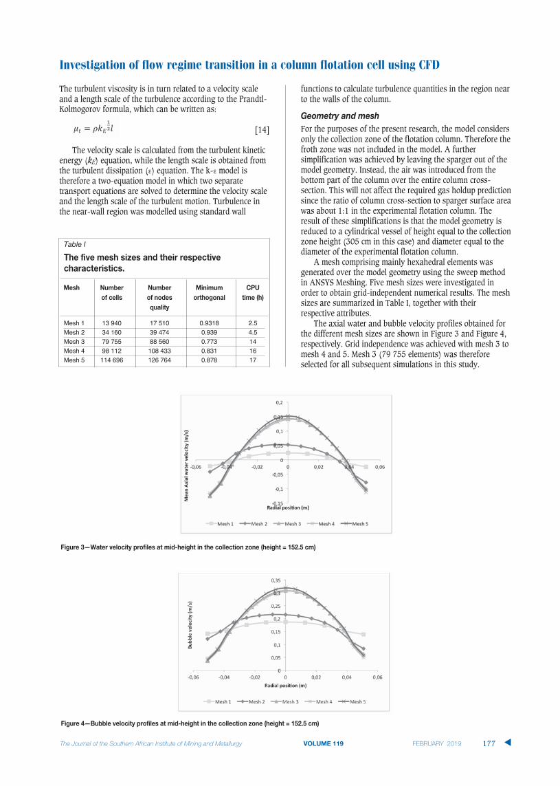
A mesh comprising mainly hexahedral elements wasgenerated over the model geometry using the sweep methodin ANSYS Meshing. Five mesh sizes were investigated inorder to obtain grid-independent numerical results. The meshsizes are summarized in Table I, together with theirrespective attributes.

The axial water and bubble velocity profiles obtained forthe different mesh sizes are shown in Figure 3 and Figure 4,respectively. Grid independence was achieved with mesh 3 tomesh 4 and 5. Mesh 3 (79 755 elements) was thereforeselected for all subsequent simulations in this study.

Investigation of flow regime transition in a column flotation cell using CFD

177 �

Table I

Mesh 1 13 940 17 510 0.9318 2.5Mesh 2 34 160 39 474 0.939 4.5Mesh 3 79 755 88 560 0.773 14Mesh 4 98 112 108 433 0.831 16Mesh 5 114 696 126 764 0.878 17

Investigation of flow regime transition in a column flotation cell using CFD

Air bubbles were introduced into the column through massand momentum source terms at the column bottom. Thesource terms were calculated from the respective superficialgas velocities and were applied over the entire column cross-section at the bottom (source) and at the top (sink) of thecollection zone.

For the liquid phase, the top of the collection zone wasmodelled as a velocity inlet boundary where inlet velocity wasspecified as equal to superficial liquid velocity Jl. Since thecomputational domain being considered is the collection zoneof the column, the superficial liquid velocity must include thefeed rate plus the bias water resulting from wash wateraddition. The superficial liquid velocity is therefore equal tothe superficial tailing rate, Jt.

The bottom part was also modelled as velocity inlet whereexit velocity was set equal to minus superficial liquid velocity.At the column wall, no slip boundary conditions were appliedfor both the air bubbles and the liquid phase.

The momentum and volume fraction equations werediscretized using the first-order upwind scheme. The first-order upwind scheme was also employed for turbulencekinetic energy and dissipation rate discretization. A time stepsize of 0.05 seconds was used in all the simulations. Thesimulations were run up to a flow time of at least 240seconds. Time averaging was carried out over the last 120seconds.

If the entire range of bubble sizes encompassing the differentflow regimes is known, CFD simulations can be conducted fora range of superficial gas velocities covering the differentflow regimes. A plot of gas holdup versus superficial gasvelocity can then be used to determine the point of departurefrom bubbly flow conditions, as described earlier. For asystem comprising water and air without frother, an empiricalformula derived by Shen (1994) can be used to calculate theSauter mean bubble size as a function of the superficial gasvelocity. However, a similar empirical equation derived forcolumn flotation conditions where frother plays an importantrole in determining the bubble size is limited to superficialgas velocities ranging from 1 to 3 cm/s. The first set of CFDresults presented in this study is therefore obtained usingbubble sizes calculated for a system without frother. The gasholdup versus superficial gas velocity relationship obtained isthen used to delineate the different flow regimes prevailing inthe column.

Once the flow regimes are identified, the evolution ofradial gas holdup profiles and gas holdup versus time graphscan be examined for the flow regimes determined from thegas holdup versus superficial gas velocity graph. Radial gasholdup profiles and gas holdup versus time graphs are thenused to determine the maximum superficial gas velocity for acolumn operating with an average bubble size of 1.5 mm,which is comparable with typical bubble sizes in industrialflotation columns. The radial gas holdup profiles wereobtained at the mid-height position (152.5 cm height) in thecolumn. On the other hand, the gas holdup versus time

graphs were obtained from a surface monitor located at thecolumn mid-height position, from which area-weightedaverage gas holdup measurements were recorded at 5-secondintervals.

It is important at this stage to clarify the definition ofregime transition and churn-turbulent flow regime as used inthe present study. Churn-turbulent flow is normallyassociated with a wide bubble size distribution, includinglarge bubbles. However, the CFD simulations in the presentresearch were conducted with a single mean bubble sizeassigned for each superficial gas velocity. Furthermore, inorder to investigate the flow regime transition for conditionsrelevant to column flotation, the other set of CFD simulationswas performed with the bubble size held at a constant valueof 1.5 mm while increasing the superficial gas velocity todetermine the maximum superficial gas velocity for thatparticular bubble size. The reference to churn-turbulent flowin the present study is therefore not based on a wide bubblesize distribution consisting of of large bubbles in thepresence of smaller ones. On the other hand, a CFD modelcoupled with a bubble population balance model can be usedto predict bubble size distributions in the column. However,bubble population balance modelling was beyond the scope ofthe present research. A possible alternative that can be usedto simulate bubble size distributions is to apply a Eulerian-Lagrangian model. This approach was not applied in thepresent study due to its higher computational cost. AEulerian-Lagrangian model would also require priorknowledge of the largest and smallest bubble sizes. Thisinformation was not readily available in the present research.

According to Lockett and Kirkpatrick (1975) there arethree main reasons for breakaway from ideal bubbly flow:flooding, liquid circulation, and the presence of large bubbles.It should therefore be possible to identify regime transitionfrom changes in the pattern and intensity of the liquidcirculation in the column even if changes in bubble size arenegligible or absent. However, the absence of large bubbles islikely to have an effect on the prediction of the location of thetransition zone as well as on the shape of the radial gasholdup profile. On the other hand, the liquid circulationpattern and its intensity depend on the prevailing radial gasholdup profile in the column (Hills, 1974).

Saddle-shaped gas holdup profiles have already beenrelated to bubbly flow conditions in two-phase flows(Kobayasi, Iida, and Kanegae, 1970; Serizawa, Kataoka, andMichiyoshi, 1975). However, the bubbly flow regime isgenerally characterized by a radially uniform gas holdupdistribution (Ruzicka et al., 2001; Vial et al., 2001; Shaikh,and Al-Dahhan, 2007). Both saddle and flat gas holdupprofiles can therefore be considered to indicate the existenceof the bubbly flow regime in the column. On the other hand,the churn-turbulent flow regime is generally distinguished bya non-uniform radial gas holdup distribution causing bulkliquid circulation. Parabolic gas holdup profiles are thereforeinterpreted to signify churn-turbulent flow conditions in thecolumn.

For the water and air only (no frother) system, CFDsimulations were carried out for superficial gas velocitiesranging from 1.01 to 14 cm/s to encompass both the bubbly

�

178

flow and churn-turbulent flow regimes. The Sauter meanbubble size for a multi-bubble system without frother (i.e.,water and air only) can be calculated as a function of thesuperficial gas velocities from the following empirical formula(Shen, 1994):

[15]

This empirical formula was derived for a laboratoryflotation column with a porous stainless steel sparger similarto the one that was used in the column modelled in thepresent work. The equation was therefore used in the presentwork to calculate the average bubble sizes that weresubsequently used in the CFD simulations.

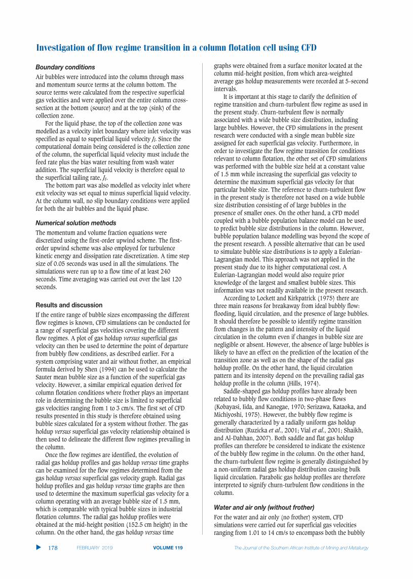
The graph of gas holdup versus superficial gas velocityobtained from CFD simulations is presented in Figure 5. Thedifferent flow regimes can be cleared delineated as follows:

� Bubbly flow regime; Jg 1.01–6.12 cm/s (linear portionof the graph)

� Transition; 6.12 < Jg 11.71 cm/s (deviation fromlinear relationship between gas holdup and superficialgas velocity)

� Churn-turbulent flow; Jg > 11.71 cm/s (third portion ofthe gas holdup versus superficial gas velocity graph).

The maximum superficial gas velocity (Jg max) beforeloss of bubbly flow is therefore equal to 6.12 cm/s for the

water and air only system without frother. This valuecompares well with the maximum superficial gas velocity of5.25 cm/s for loss of bubbly flow predicted from drift fluxtheory by Xu, Finch, and Uribe-Salas (1991).

Having delineated the different flow regimes using thegas holdup versus superficial gas velocity relationship, theevolution of the radial gas holdup profiles was examined as the superficial gas velocity increased from 1.01 cm/s to 14 cm/s.

A number of different types of radial gas holdup profiles wereobtained from the CFD simulations, including saddle-shaped,flat, and parabolic profiles. These profiles were then related tothe flow regimes defined from the gas holdup/superficial gasvelocity relationship (Figure 5).

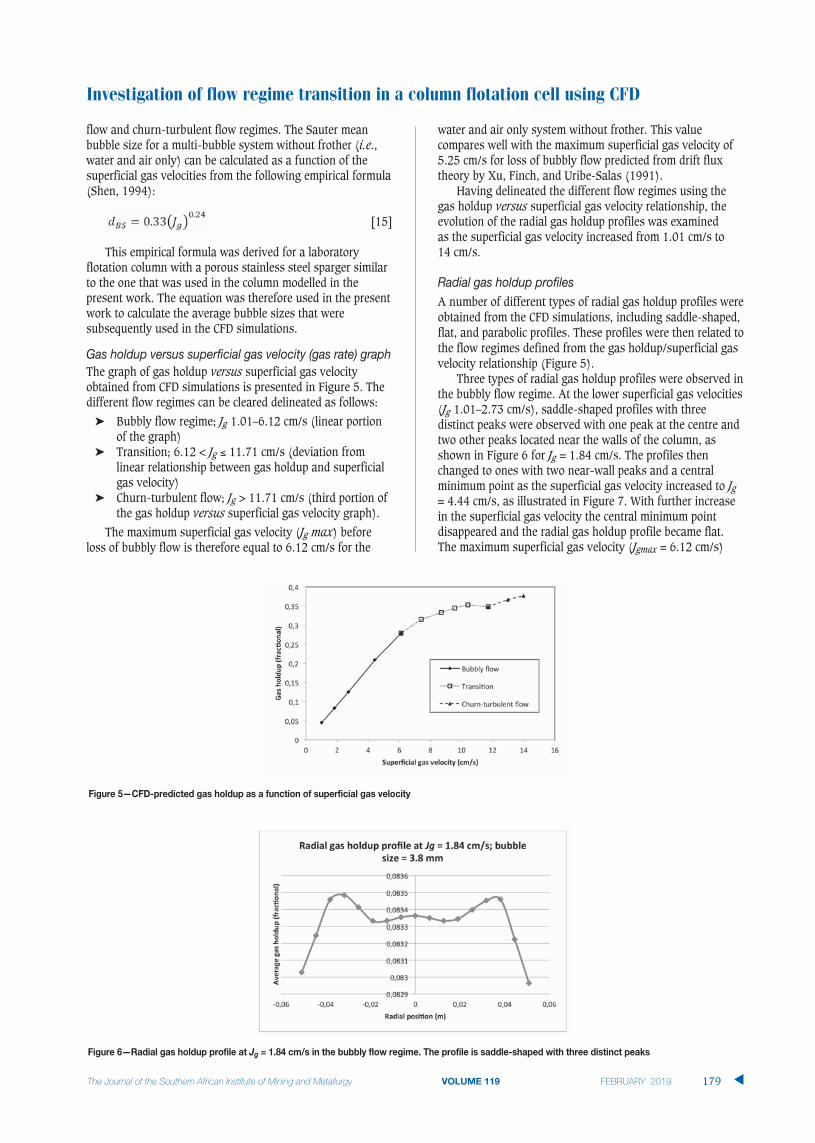
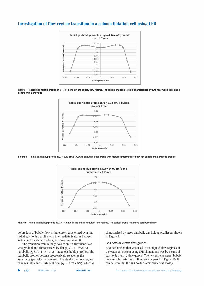
Three types of radial gas holdup profiles were observed inthe bubbly flow regime. At the lower superficial gas velocities(Jg 1.01–2.73 cm/s), saddle-shaped profiles with threedistinct peaks were observed with one peak at the centre andtwo other peaks located near the walls of the column, asshown in Figure 6 for Jg = 1.84 cm/s. The profiles thenchanged to ones with two near-wall peaks and a centralminimum point as the superficial gas velocity increased to Jg= 4.44 cm/s, as illustrated in Figure 7. With further increasein the superficial gas velocity the central minimum pointdisappeared and the radial gas holdup profile became flat.The maximum superficial gas velocity (Jgmax = 6.12 cm/s)

Investigation of flow regime transition in a column flotation cell using CFD

179 �

Investigation of flow regime transition in a column flotation cell using CFD

before loss of bubbly flow is therefore characterized by a flatradial gas holdup profile with intermediate features betweensaddle and parabolic profiles, as shown in Figure 8.

The transition from bubbly flow to churn-turbulent flowwas gradual and characterized by flat (Jg = 7.41 cm/s) toparabolic (Jg 8.70–11.71 cm/s) radial gas holdup profiles. Theparabolic profiles became progressively steeper as thesuperficial gas velocity increased. Eventually the flow regimechanges into churn-turbulent flow (Jg > 11.71 cm/s), which is

characterized by steep parabolic gas holdup profiles as shownin Figure 9.

Another method that was used to distinguish flow regimes inthe water–air system using CFD simulations was by means ofgas holdup versus time graphs. The two extreme cases, bubblyflow and churn-turbulent flow, are compared in Figure 10. Itcan be seen that the gas holdup versus time was mostly

�

180

constant in the bubbly flow regime (Jg = 1.84 cm/s), while verywide variations in gas holdup were observed in the churn-turbulent flow regime (i.e., Jg = 14 cm/s). The transition frombubbly flow to churn-turbulent flow pattern was gradual andcharacterized by moderate to large fluctuations in gas holdup,with the gas holdup variations becoming increasingly intenseas the superficial gas velocity increased.

The results from the CFD simulations of the water and aironly (no frother) system, where bubble sizes are calculatedfrom the superficial gas velocity according to Equation [15],are summarized in Table II. The progression from bubblyflow conditions to churn-turbulent flow can also be clearlyappreciated from this table. The distinguishing characteristicsof the flow regimes are summarized in Table III.

Investigation of flow regime transition in a column flotation cell using CFD

181 �

Table II

1.01 0.33 0.045 Saddle with three peaks Constant Bubbly flow1.84 0.38 0.083 Saddle with three peaks Constant Bubbly flow2.73 0.42 0.125 Saddle with three peaks Almost constant Bubbly flow4.44 0.47 0.209 Saddle profile with Almost constant Bubbly flow

two near-wall peaks6.12 0.51 0.279 Flat profile with Small to moderate Bubbly flow

intermediate features variations (maximum superficialbetween parabolic gas velocity)and saddle profiles

7.41 0.53 0.315 Flat Moderate variations Transition8.70 0.55 0.333 Flat-like parabolic Moderate variations Transition9.56 0.57 0.345 Parabolic Significant variations Transition10.42 0.58 0.353 Parabolic Significant variations Transition11.71 0.60 0.348 Steep parabolic Large variations Transition (last point)13.00 0.61 0.367 Steep parabolic Wide variations Churn-turbulent flow

(large variations)14.00 0.62 0.377 Steep parabolic Wide variations Churn-turbulent flow

(large variations)

Table III

Bubbly flow • Characterized by saddle-shaped radial gas holdup profiles accompanied by a constant gas holdup versus time graph• The profiles at lower Jg have three peaks that give way to profiles with two near-wall peaks and a central minimum and eventually

flat profiles as Jg increases Transition • Characterized by flat to parabolic gas holdup profiles

• The profiles become increasingly steep with increasing Jg while gas holdup versus time varies from moderate to large fluctuationsChurn-turbulent flow • Characterized by steep parabolic profiles with very wide variations in gas holdup versus time

Investigation of flow regime transition in a column flotation cell using CFD

In flotation columns, the bubble size depends not only on thesuperficial gas velocity, but also on other physical chemicalcharacteristics of the gas-liquid system. In this case, thebubble size can be calculated as a function of the superficialgas velocity according to the following relationship (Finchand Dobby, 1990; Yianatos and Finch, 1990).

[16]

where C and n are constants. The constant C is a fittingparameter which depends mainly on frother concentration,the sparger size, and column size. Simulations were carriedout for the experimental conditions used by Xu, Finch, andUribe-Salas (1991) and Xu et al. (1989), particularly the casein which the frother concentration was 10 ppm. The value ofC was therefore equal to unity while n was 0.25.

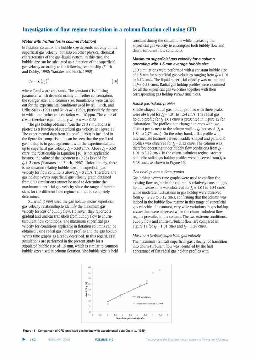
The gas holdup obtained from the CFD simulations isplotted as a function of superficial gas velocity in Figure 11.The experimental data from Xu et al. (1989) is included inthe figure for comparison. It can be seen that the predictedgas holdup is in good agreement with the experimental dataup to superficial gas velocity Jg = 3.60 cm/s. Above Jg = 3.60cm/s, the relationship in Equation [16] is not applicablebecause the value of the exponent n (0.25) is valid for Jg 1–3 cm/s (Yianatos and Finch, 1990). Unfortunately, thereis no equation relating bubble size and superficial gasvelocity for flow conditions above Jg = 3 cm/s. Therefore, thegas holdup versus superficial gas velocity graph obtainedfrom CFD simulations cannot be used to determine themaximum superficial gas velocity since the range of bubblesizes for the different flow regimes cannot be completelydetermined.

Xu et al. (1989) used the gas holdup versus superficialgas velocity relationship to identify the maximum gasvelocity for loss of bubbly flow. However, they reported agradual and unclear transition from bubbly flow to churn-turbulent flow conditions. The maximum superficial gasvelocity for conditions applicable in flotation columns can beobtained using radial gas holdup profiles and the gas holdupversus time graphs as already described. In this regard, CFDsimulations are performed in the present study for astipulated bubble size of 1.5 mm, which is similar to commonbubble sizes used in column flotation. The bubble size is held

constant during the simulations while increasing thesuperficial gas velocity to encompass both bubbly flow andchurn-turbulent flow conditions.

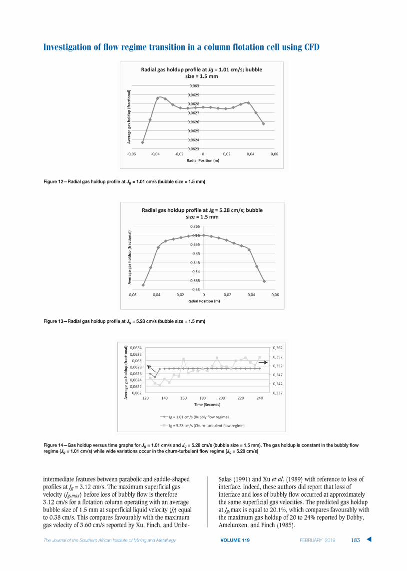
CFD simulations were performed with a constant bubble sizeof 1.5 mm for superficial gas velocities ranging from Jg = 1.01to 6.12 cm/s. The liquid superficial velocity was maintainedat Jl = 0.38 cm/s. Radial gas holdup profiles were examinedfor all the superficial gas velocities together with theircorresponding gas holdup versus time plots.

Saddle-shaped radial gas holdup profiles with three peakswere observed for Jg = 1.01 to 1.54 cm/s. The radial gasholdup profile for Jg 1.01 cm/s is presented in Figure 12 forelaboration. The profiles then changed to ones with twodistinct peaks near to the column wall as Jg increased (Jg =1.84 to 2.73 cm/s). On the other hand, a flat profile withintermediate features between saddle-shaped and parabolicprofiles was observed for Jg = 3.12 cm/s. The column wastherefore operating under bubbly flow conditions from Jg =1.01 to 3.12 cm/s. In the churn-turbulent regime, steeperparabolic radial gas holdup profiles were observed from Jg =5.28 cm/s, as shown in Figure 13.

Gas holdup versus time graphs were used to confirm theexisting flow regime in the column. A relatively constant gasholdup versus time was observed for Jg = 1.01 to 1.84 cm/swhile moderate fluctuations in gas holdup were observedfrom Jg = 2.28 to 3.12 cm/s, confirming that the column wasindeed in the bubbly flow regime in this range of superficialgas velocities. In contrast, very wide variations in gas holdupversus time were observed when the churn-turbulent flowregime prevailed in the column. The two extreme conditions,bubbly flow and churn-turbulent flow, are compared inFigure 14 for Jg = 1.01 cm/s and Jg = 5.28 cm/s.

The maximum (critical) superficial gas velocity for transitioninto churn-turbulent flow was identified by the firstappearance of flat radial gas holdup profiles with

�

182

et al

intermediate features between parabolic and saddle-shapedprofiles at Jg = 3.12 cm/s. The maximum superficial gasvelocity (Jg,max) before loss of bubbly flow is therefore 3.12 cm/s for a flotation column operating with an averagebubble size of 1.5 mm at superficial liquid velocity (Jl) equalto 0.38 cm/s. This compares favourably with the maximumgas velocity of 3.60 cm/s reported by Xu, Finch, and Uribe-

Salas (1991) and Xu et al. (1989) with reference to loss ofinterface. Indeed, these authors did report that loss ofinterface and loss of bubbly flow occurred at approximatelythe same superficial gas velocities. The predicted gas holdupat Jg,max is equal to 20.1%, which compares favourably withthe maximum gas holdup of 20 to 24% reported by Dobby,Amelunxen, and Finch (1985).

Investigation of flow regime transition in a column flotation cell using CFD

183 �

Investigation of flow regime transition in a column flotation cell using CFD

The radial gas holdup profile at Jg,max is shown in Figure15, and its corresponding gas holdup versus time graph inFigure 16. It can be seen that the maximum superficial gasvelocity is characterized by a flat gas holdup profileaccompanied by moderate gas holdup fluctuations. Theresults from the CFD simulations for 1.5 mm bubble size aresummarized in Table IV. The progression from bubblyflow conditions to churn-turbulent flow can be clearly seen inthe table.

Two different flow patterns were observed, depending onsuperficial gas velocity and bubble size. With increasingsuperficial gas velocity the well-known ‘Gulf Stream’circulation pattern, in which the liquid rises in the centre ofthe column and descends near the column wall, wasobserved. In contrast, an ‘inverse’ circulation flow pattern, inwhich the liquid rises near the column wall but descends in

�

184

Table IV

1.01 6.27 Saddle-shaped with three peaks Constant Bubbly flow1.54 9.66 Saddle-shaped with three peaks - Bubbly flow1.84 11.60 Saddle-shaped with two peaks Very small variations Bubbly flow2.28 14.47 Saddle-shaped with two peaks Moderate fluctuations Bubbly flow2.73 17.46 Saddle-shaped with two peaks Moderate fluctuations Bubbly flow3.12 20.10 Flat, intermediate between saddle and parabolic profiles Moderate fluctuations Bubbly flow (Jgmax)3.60 23.23 Flat profile Larger fluctuations Transition 4.03 26.27 Parabolic profile Larger fluctuations Transition4.44 29.05 Parabolic Large variations Transition5.28 35.51 Steep parabolic Very large variations Churn-turbulent flow

the centre and immediately adjacent to the walls, occurred atlower superficial gas velocities. This is the first study toreport such an inverse flow pattern in column flotation.However, similar flow reversals have been observed inexperimental work on fluidized bed reactors (Lin, Chen, andChao, 1985).

The inverse circulation pattern has been theoreticallyinvestigated in bubble columns and is associated with fullydeveloped saddle-shaped radial gas holdup profiles (Clark,Atkinson, C., and Flemmer, 1987; Clark, van Egmond, andNebiolo E. 1990). In the present study, the inverse circulationpattern was observed at Jg = 1.01 cm/s and Jg = 1.54 cm/s forsimulations with bubble size = 1.5 mm and superficial liquidvelocity = 0.38 cm/s. Saddle-shaped gas holdup profiles withtwo distinct peaks near the walls of the column were alsopresent under these conditions. The liquid velocity vectorplots obtained from CFD simulations are presented in Figure17 and Figure 18 for the two circulation patterns.

Clark, van Egmond, and Nebiolo (1990) have describedthe sequence of events that may initiate liquid circulation inbubble columns. In general, liquid circulation in bubblecolumns is initiated by density differences in the gas-liquidmixture, depending on the prevailing radial gas holdupprofile. If the concentration of air bubbles is higher in thecentral part of the column compared to the outer annularregion, the mean density of the mixture will be lower near thecentre of the column than in the outer annulus. Thehydrostatic pressure head will therefore be higher in theouter annulus, hence a radial pressure difference is set upinside the column. This will cause an inward radialmovement of liquid and initiate liquid circulation. The inversecirculation pattern will occur if the concentration of bubbles ishigher in the outer annular region, as in the case of saddle-shaped gas holdup profiles.

In this study, the evolution of the shape of the radial gasholdup profile in a pilot-scale flotation column was studiedusing CFD to delineate the maximum gas velocity for loss ofbubbly flow. With increasing superficial gas velocity, the gasholdup profile passes through different stages, which can beused to define the prevailing flow regime in the column. Thedifferent flow regimes were also verified by the intensity ofthe local variations of the gas holdup.

In the bubbly flow regime, saddle-shaped and flat radialgas holdup profiles were obtained. These profiles wereaccompanied by minor to moderate gas holdup variations inthe column. The transition regime was gradual andcharacterized by flat to parabolic gas holdup profiles. Theparabolic profiles became progressively steeper as thesuperficial gas velocity increased. The corresponding gasholdup versus time graphs in the transition regime showedmoderate to wide variations in gas holdup. On the otherhand, the churn-turbulent flow regime was distinguished bysteep parabolic gas holdup profiles with very wide variationsin gas holdup versus time.

For conditions relevant to column flotation, the maximumsuperficial gas velocity was determined for a columnoperating with an average bubble size of 1.5 mm andsuperficial liquid velocity equal to 0.38 cm/s. The maximumsuperficial gas velocity was found to be equal to 3.12 cm/s.The corresponding maximum gas holdup value was 20.1%.

Two possible flow patterns were revealed in the simulatedcolumn in this study: the ‘Gulf Stream’ circulation patternand an inverse circulation pattern. The latter was observedonly in the presence of fully developed saddle-shaped radialgas holdup profiles.

Investigation of flow regime transition in a column flotation cell using CFD

185 �

Investigation of flow regime transition in a column flotation cell using CFD

The CFD simulations in the present study assumed aconstant average bubble size for the flotation column.However, for the churn-turbulent regime, a bubble sizedistribution exists that could have an effect on thehydrodynamics of the column. CFD models coupled with abubble population balance model should therefore beconsidered in future studies in order to account for bubblesize distributions in the transition and churn-turbulent flowregimes.

The authors would like to acknowledge the Centre forInternational Cooperation at VU University Amsterdam (CIS-VU) and the Copperbelt University (CBU) for providing thescholarship and subsequent funding for this research throughthe Nuffic-HEART Project. We would also like toacknowledge the Process Engineering Department atStellenbosch University for providing the necessary facilitiesthat made this research possible. The CFD simulations in ourstudies were performed using the University of Stellenbosch'sRhasatsha High Performance Computing (HPC) cluster:http://www.sun.ac.za/hpc

CD Drag coefficient, dimensionlessdB Bubble diameter, mmdBS Sauter mean bubble size(FD) Drag force per unit volume, N/m3

g Gravitational acceleration, 9.81 m/s2

Jg Superficial gas velocity, cm/sJg,max Maximum superficial gas velocityJl Superficial liquid velocitykE Turbulence kinetic energy, m2/s2

P Pressure, PaRe Reynolds number, dimensionlessSk Mass source term for phase k, kg/m3-su Reynolds averaged velocity, m/su' Velocity fluctuation, m/s

G Air volume fraction or gas holdupVolume fractionTurbulence dissipation rate, m2/s3

RT Rayleigh-Taylor instability wavelengthViscosity, kg/m-s

t Turbulent viscosity, kg/m-sDensity, kg/m3

Surface tension (N/m)k Viscous stress tensor, Pa

B BubbleD DragG, g Gasi, j Spatial directionsk PhaseL, l Liquid

CLARK, N., ATKINSON, C., and FLEMMER, R. 1987. Turbulent circulation in bubblecolumns. AIChE Journal, vol. 33, no. 3. pp. 515–518.

CLARK, N., VAN EGMOND, J., and NEBIOLO E. 1990. The drift-flux model applied tobubble columns and low velocity flows. International Journal ofMultiphase Flow, vol. 16, no. 2. pp. 261–279.

DOBBY, G., AMELUNXEN, R., and FINCH, J. 1985. Column flotation: Some plantexperience and model development. Proceedings of the First IFACSymposium on Automation for Mineral Resource Development, Brisbane,Australia, 9–11 July. IFAC Proceedings, vol. 18, no. 6. pp. 259–263.

FINCH, J.A. and DOBBY, G.S. 1990. Column Flotation. Pergamon, Oxford, UK.

HILLS, J. 1974. Radial non-uniformity of velocity and voidage in a bubblecolumn. Transactions of the Institution of Chemical Engineers, vol. 52, no. 1. pp. 1–9.

ITYOKUMBUL, M. 1992. A new modelling approach to flotation column desing .Minerals Engineering, vol. 5, no. 6. pp. 685–693.

KOBAYASI, K., IIDA, Y., and KANEGAE, N. 1970. Distribution of local void fractionof air-water two-phase flow in a vertical channel. Bulletin of JSME, vol. 13, no. 62. pp. 1005–1012.

KOLEV, N.I. 2005. Multiphase Flow Dynamics 2: Thermal and MechanicalInteractions. 2nd edn. Vol. 2. Springer, Berlin, Germany.

LANGBERG, D. and JAMESON, G. 1992. The coexistence of the froth and liquidphases in a flotation column. Chemical Engineering Science, vol. 47, no. 17. pp. 345–355.

LIN. J., CHEN, M., and CHAO, B. 1985. A novel radioactive particle trackingfacility for measurement of solids motion in gas fluidized beds. AIChEJournal, vol. 31, no. 3. pp. 465–73.

LOCKETT, M. and KIRKPATRICK, R. 1975. Ideal bubbly flow and actual flow inbubble columns. Transactions of the Institution of Chemical Engineers,vol. 53. pp. 267–273.

MECKLENBURG, M.M. 1992. Hydrodynamic study of a downwards concurrentbubble column. MEng dissertation, McGill University, Montreal, Canada.

RUZICKA, M., ZAHRADNIK, J., DRAHOŠ, J., and THOMAS N. 2001. Homogeneous–heterogeneous regime transition in bubble columns. Chemical EngineeringScience, vol. 56, no. 15. pp. 4609–4626.

SERIZAWA, A., KATAOKA, I., and MICHIYOSHI, I. 1975. Turbulence structure of air-water bubbly flow – II. local properties. International Journal ofMultiphase Flow, vol. 2, no. 3. pp. 235–246.

SHAIKH, A. and AL-DAHHAN, M.H. 2007. A review on flow regime transition inbubble columns. International Journal of Chemical Reactor Engineering,vol. 5, no. 1. https://doi.org/10.2202/1542-6580.1368

SHEN, G. 1994. Bubble swarm velocities in a flotation column. PhD dissertation,McGill University; Montreal, Canada.

SUMMERS, A.J. 1995. A study of the operating variables of the Jameson cell.MEng dissertation, McGill University, Montreal, Canada.

VIAL, C., PONCIN, S., WILD, G., and MIDOUX, N. 2001. A simple method for regimeidentification and flow characterisation in bubble columns and airliftreactors. Chemical Engineering and Processing: Process Intensification,vol. 40, no. 2. pp. 135–151.

XU, M., FINCH, J., and URIBE-SALAS, A. 1991. Maximum gas and bubble surfacerates in flotation columns. International Journal of Mineral Processing,vol. 32, no. 3. pp. 233–250.

XU, M., Uribe-Salas, A., Finch, J., and Gomez, C. 1989. Gas rate limitation incolumn flotation. Processing of Complex Ores: Proceedings of theInternational Symposium on Processing of Complex Ores, Halifax, NovaScotia, 20-24 August 1989. Elsevier. pp. 397–407.

YIANATOS, J. and FINCH, J. 1990. Gas holdup versus gas rate in the bubblyregime. International Journal of Mineral Processing, vol. 29, no. 1. pp. 141–146. �

�

186