V11: Structure Learning in Bayesian Networks In lectures V9 and V10 we made the strong assumption...
42
V11: Structure Learning in Bayesian Networks In lectures V9 and V10 we made the strong assumption that we know in advance the network structure. Today, we consider the task of learning in situations where we do not know the structure of the BN in advance. Instead, we will apply the strong assumption that our data set is fully observed. As before, we assume that the data D are generated IID from an underlying distribution P*(X). We assume that P* is induced by some Bayesian network G* over X. 1 SS 2014 - lecture 11 Mathematics of Biological Networks
-
Upload
warren-ramsey -
Category
Documents
-
view
217 -
download
0
Transcript of V11: Structure Learning in Bayesian Networks In lectures V9 and V10 we made the strong assumption...
V11: Structure Learning in Bayesian Networks
In lectures V9 and V10 we made the strong assumption
that we know in advance the network structure.
Today, we consider the task of learning in situations
where we do not know the structure of the BN in advance.
Instead, we will apply the strong assumption that our data set is fully observed.
As before, we assume that the data D are generated IID
from an underlying distribution P*(X).
We assume that P* is induced by some Bayesian network G* over X.
1SS 2014 - lecture 11 Mathematics of Biological Networks
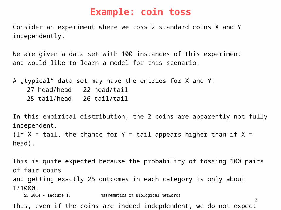
Example: coin toss
Consider an experiment where we toss 2 standard coins X and Y independently.
We are given a data set with 100 instances of this experiment
and would like to learn a model for this scenario.
A „typical“ data set may have the entries for X and Y:
27 head/head 22 head/tail
25 tail/head 26 tail/tail
In this empirical distribution, the 2 coins are apparently not fully independent.
(If X = tail, the chance for Y = tail appears higher than if X = head).
This is quite expected because the probability of tossing 100 pairs of fair coins
and getting exactly 25 outcomes in each category is only about 1/1000.
Thus, even if the coins are indeed indepdendent, we do not expect that
the observed empirical distribution will satisfy independence.
2SS 2014 - lecture 11 Mathematics of Biological Networks

Example: coin toss
Suppose we get the same results in a very different situation.
Say we scan the sports section of our local newspaper for 100 days
and choose an article at random each day.
We mark X = x1 if the word „rain“ appears in the article and X = x0 otherwise.
Similarly, Y denotes whether the word „football“ appears in the article.
Our intuition whether the two random variables are independent is unclear.
If we get the same empirical counts as in the coins described before,
we might suspect that there is some weak connection.
In other words, it is hard to be sure whether the true underlying
model has an edge between X and Y or not.
3SS 2014 - lecture 11 Mathematics of Biological Networks
Goals of the learning process
The goal of learning G* from the data is hard to achieve because - the data sampled from P* are typically noisy and - do not reconstruct P* perfectly.
We cannot detect with complete reliability which
independencies are present in the underlying distribution.
Therefore, we must generally make a decision about our willingness
to include in our learned model edges about which we are less sure.
If we include more of these edges, we will often learn
a model that contains spurious edges.
If we include few edges, we may miss independencies.
The decision which compromise is better depends on the application.
4SS 2014 - lecture 11 Mathematics of Biological Networks

Independence in coin toss example?
It seems that if we do make mistakes in the structure, it is better to have
too many rather than too few edges. But the situation is more complex.
Let‘s go back to the coin example and assume that we had only 20 cases for X/Y:
3 head/head 6 head/tail
5 tail/head 6 tail/tail
When we assume X and Y as correlated, we find by MLE
(where we simply count the observed numbers):
P(X = H) = 9/20 = 0.45
P(Y = H | X = H) = 3/9 = 1/3
P(Y = H | X = T) = 5/11
In the independent structure (no edge between X and Y), P(Y = H) = 8/20 = 0.4
5SS 2014 - lecture 11 Mathematics of Biological Networks

Noisy data → prefer sparse models
All of these parameter estimates are imperfect, of course.
The ones in the more complex model are significantly more likely to be skewed
(dt: verzogen) because each one is estimated from a much smaller data set.
E.g. P(Y = H | X = H) is estimated from only 9 instances
compared to 20 instances for the estimation of P(Y = H).
Note that the standard estimation error of MLE is .
When doing density estimation from limited data,
it is often better to prefer a sparser structure.
6SS 2014 - lecture 11 Mathematics of Biological Networks

Overview of structure learning methods
Roughly speaking, there are 3 approaches to learning
without a prespecified structure:
(1) constraint-based structure learning
Finds a model that best explains the dependencies/independencies in the data.
(2) Score-based stucture learning (today)
We define a hypothesis space of potential models and a scoring function
that measures how well the model fits the observed data.
Our computational task is then to find the highest-scoring network.
(3) Bayesian model averaging methods
Generates an ensemble of possible structures.
7SS 2014 - lecture 11 Mathematics of Biological Networks
Structure Scores
We will discuss 2 obvious choices of scoring functions:- Maximum likelihood parameters (today)- Bayesian scores (V12)
Maximum likelihood parameters
This function measures the probability of the data given a model.
→ try to find a model that would make the data as probable as possible.
A model is a pair G, G.
Our goal is to find both a graph G and parameters G
that maximize the likelihood.
8SS 2014 - lecture 11 Mathematics of Biological Networks
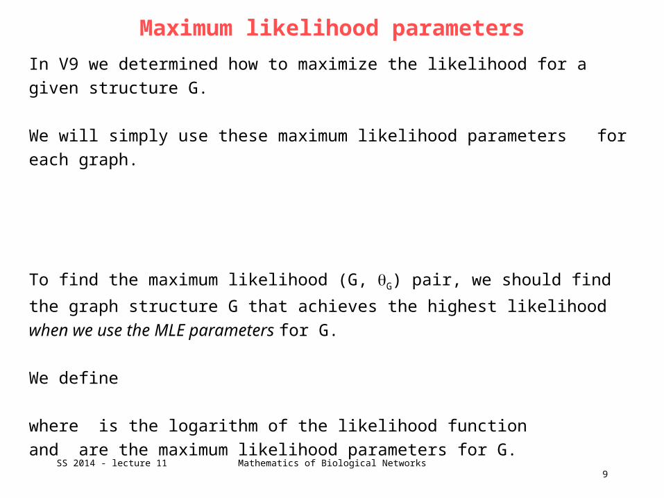
Maximum likelihood parameters
In V9 we determined how to maximize the likelihood for a given structure G.
We will simply use these maximum likelihood parameters for each graph.
To find the maximum likelihood (G, G) pair, we should find the graph structure G
that achieves the highest likelihood when we use the MLE parameters for G.
We define
where is the logarithm of the likelihood function
and are the maximum likelihood parameters for G.
9SS 2014 - lecture 11 Mathematics of Biological Networks

Maximum likelihood parameters
Let us consider again the scenario of the 2 coins.
In model G0, X and Y are assumed to be independent. In this case, we get
In model G1, we assume a dependency modelled by the arc X → Y. We get
where is the maximum likelihood estimate for P(x)
and is the maximum likelihood estimate for P(y | x).
The scores of the two models share a common component, the first term.
10SS 2014 - lecture 11 Mathematics of Biological Networks
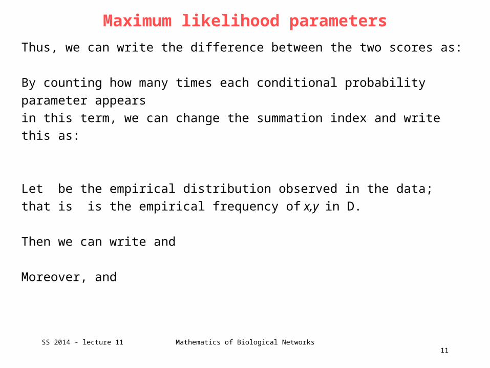
Maximum likelihood parameters
Thus, we can write the difference between the two scores as:
By counting how many times each conditional probability parameter appears
in this term, we can change the summation index and write this as:
Let be the empirical distribution observed in the data;
that is is the empirical frequency of x,y in D.
Then we can write and
Moreover, and
11SS 2014 - lecture 11 Mathematics of Biological Networks
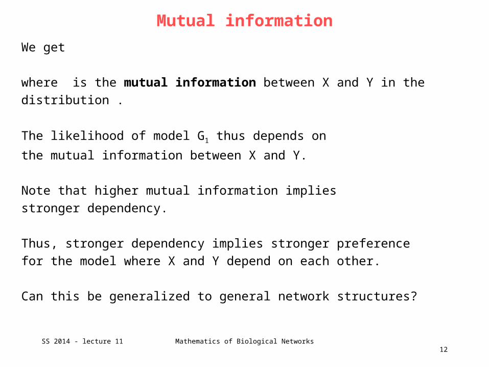
Mutual information
We get
where is the mutual information between X and Y in the distribution .
The likelihood of model G1 thus depends on
the mutual information between X and Y.
Note that higher mutual information implies
stronger dependency.
Thus, stronger dependency implies stronger preference
for the model where X and Y depend on each other.
Can this be generalized to general network structures?
12SS 2014 - lecture 11 Mathematics of Biological Networks
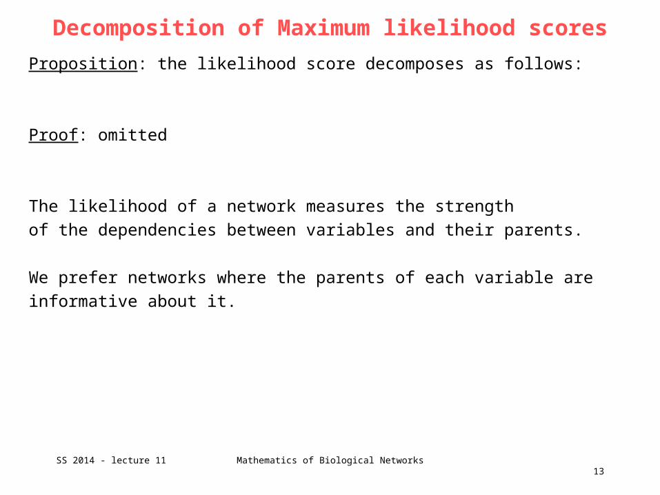
Decomposition of Maximum likelihood scores
Proposition: the likelihood score decomposes as follows:
Proof: omitted
The likelihood of a network measures the strength
of the dependencies between variables and their parents.
We prefer networks where the parents of each variable are informative about it.
13SS 2014 - lecture 11 Mathematics of Biological Networks

Maximum likelihood parameters
We can also express this result in a complementary manner.
Corollorary: Let X1, …, Xn be an ordering of the variables
that is consistent with edges in G. Then
The first term on the right-hand-side does not depend
on the structure, but the second term does.
The second term involves conditional mutual-information
of variable Xi and the preceding variables given the parents of Xi.
14SS 2014 - lecture 11 Mathematics of Biological Networks

Limitations of the maximum likelihood score
The likelihood score is a good measure
of the fit of the estimated BN and the training data.
Important, however, is the performance of the learned network on new instances.
It turns out that the MLE score never prefers simpler networks over more complex
networks. The optimal ML network will always be a fully connected network.
Thus, the ML overfits the training data.
The model often does not generalize well to new data cases.
15SS 2014 - lecture 11 Mathematics of Biological Networks
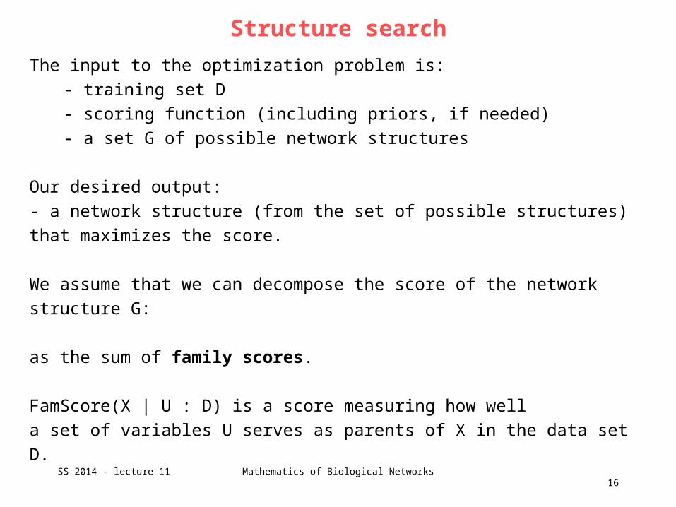
Structure search
The input to the optimization problem is:
- training set D
- scoring function (including priors, if needed)
- a set G of possible network structures
Our desired output:
- a network structure (from the set of possible structures) that maximizes the score.
We assume that we can decompose the score of the network structure G:
as the sum of family scores.
FamScore(X | U : D) is a score measuring how well
a set of variables U serves as parents of X in the data set D.
16SS 2014 - lecture 11 Mathematics of Biological Networks

Tree-structure networks
Structure learning of tree-structure networks is the simplest case.
Definition: in tree-structured network structures G,
each variable X has at most one parent in G.
The advantage of trees is that they can be learned efficiently in polynomial time.
Learning a tree model is often used as a starting point
for learning more complex structures.
Key properties to be used:
- decomposability of the score
- restriction on the number of parents
17SS 2014 - lecture 11 Mathematics of Biological Networks
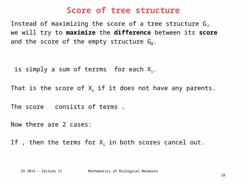
Score of tree structure
Instead of maximizing the score of a tree structure G,
we will try to maximize the difference between its score
and the score of the empty structure G0.
is simply a sum of terrms for each Xi.
That is the score of Xi if it does not have any parents.
The score consists of terms .
Now there are 2 cases:
If , then the terms for Xi in both scores cancel out.
18SS 2014 - lecture 11 Mathematics of Biological Networks

Structure search
If we are left with the difference between the 2 terms.
If we define the weight
then we see that (G) is the sum of weights on pairs , such that in G
We have thus transformed our problem to one of finding
a maximum weight spanning forest in a directed weighted graph.
19SS 2014 - lecture 11 Mathematics of Biological Networks

General case
For a general model topology that may also involve cycles,
we start by considering the search space.
We can think of the search space as a graph
over candidate solutions (different network topologies).
Nodes are connected by operators that transform one network into the other one.
If each state has few neighbors, the search procedure only
has to consider few solutions at each point of the search.
However, the search for an optimal (or high-scoring) solution
may be long and complex.
On the other hand, if each state has many neighbors, the search may involve
only a few steps, but it may be difficult to decide at each step which point to take.
20SS 2014 - lecture 11 Mathematics of Biological Networks

General case
A good trade-off for this problem chooses reasonably few neighbors for each state
but ensures that the „diameter“ of the search space remains small.
A natural choice for the neighbors of a state is a set of structures
that are identical to it except for small „local“ modifications.
We will consider the following set of modifications of this sort:
- Edge addition- Edge deletion- Edge reversal
The diameter of the search space is then at most n2.
(We could first delete all edges in G1 that do not appear in G2 and then add the edges of G2
that are not in G1. This is bounded by the total number of possible edges n2).
21SS 2014 - lecture 11 Mathematics of Biological Networks
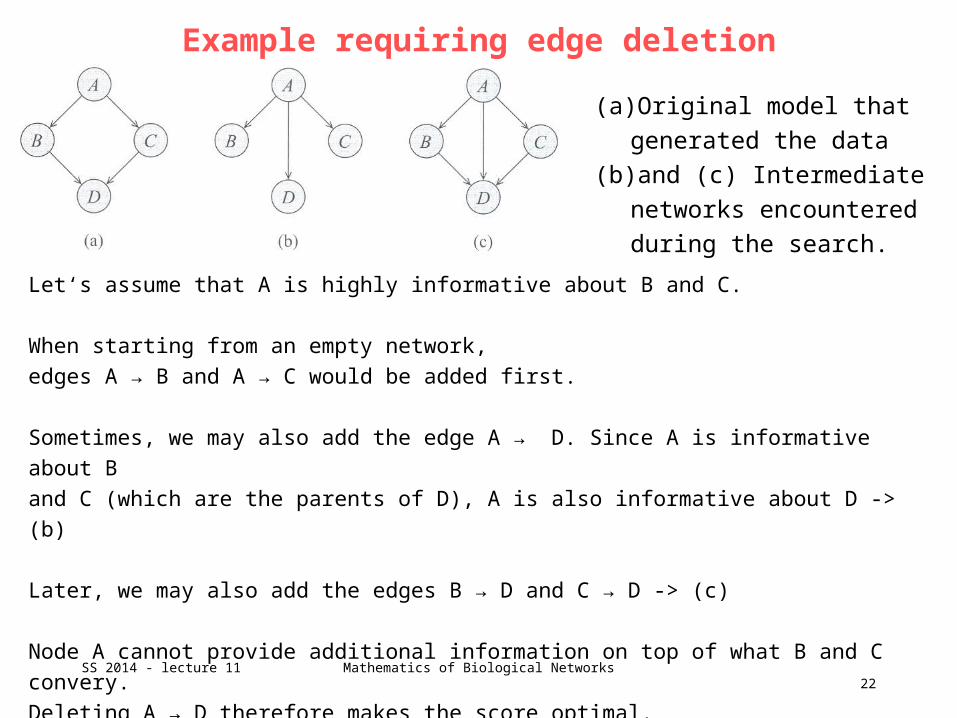
Example requiring edge deletion
22SS 2014 - lecture 11 Mathematics of Biological Networks
Let‘s assume that A is highly informative about B and C.
When starting from an empty network,
edges A → B and A → C would be added first.
Sometimes, we may also add the edge A → D. Since A is informative about B
and C (which are the parents of D), A is also informative about D -> (b)
Later, we may also add the edges B → D and C → D -> (c)
Node A cannot provide additional information on top of what B and C convery.
Deleting A → D therefore makes the score optimal.
(a) Original model that
generated the data
(b) and (c) Intermediate
networks encountered
during the search.

Example requiring edge reversal
23SS 2014 - lecture 11 Mathematics of Biological Networks
(a) Original network, (b) and (c) intermediate networks during search.
(d) Undesirable outcome.
When adding edges, we do not know their direction because both directions give
the same score.
This is where edge reversal helps.
In situation (c) we realize that A and B together should make the best prediction of
C. Therefore, we need to reverse the direction of the arc pointing at A.

24
Who controls thedevelopmental status of a cell?
SS 2014 - lecture 11 Mathematics of Biological Networks
We will continue with structure learning in V12
25
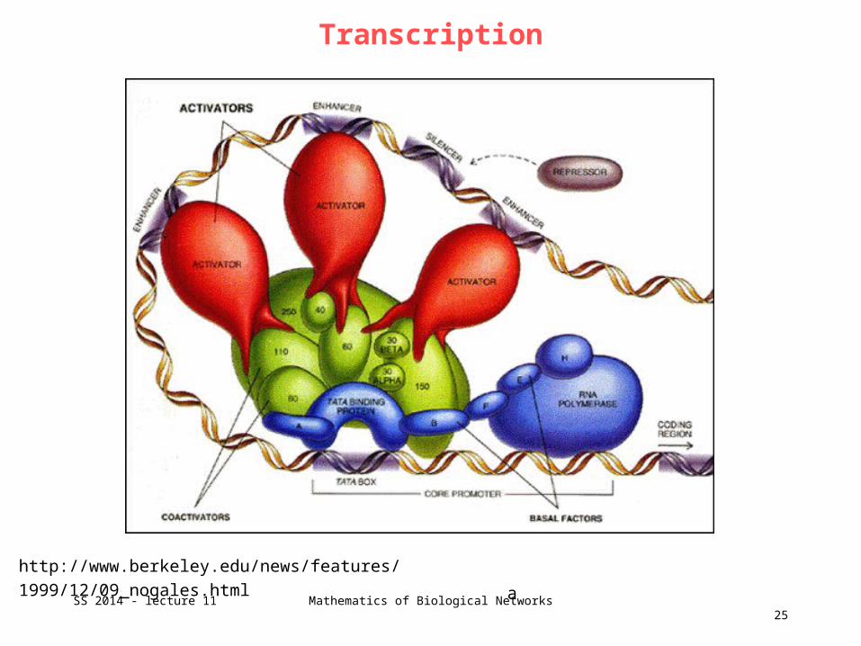
Transcription
a
http://www.berkeley.edu/news/features/1999/12/09_nogales.html
SS 2014 - lecture 11 Mathematics of Biological Networks
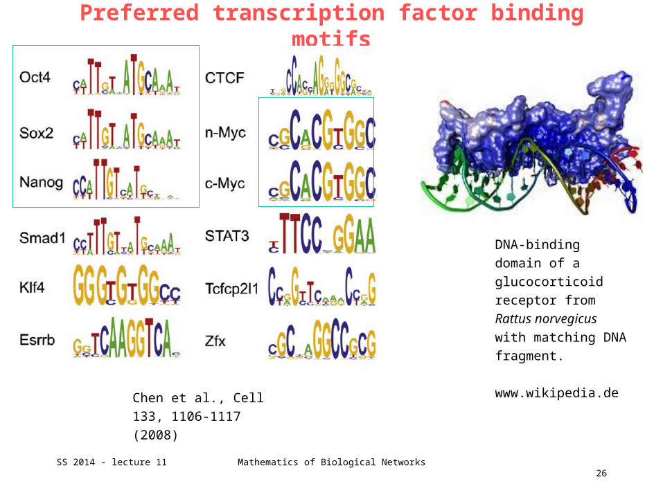
Preferred transcription factor binding motifs
Chen et al., Cell 133,
1106-1117 (2008)
26
DNA-binding domain
of a glucocorticoid
receptor from
Rattus norvegicus
with matching DNA
fragment.
www.wikipedia.de
SS 2014 - lecture 11 Mathematics of Biological Networks
27
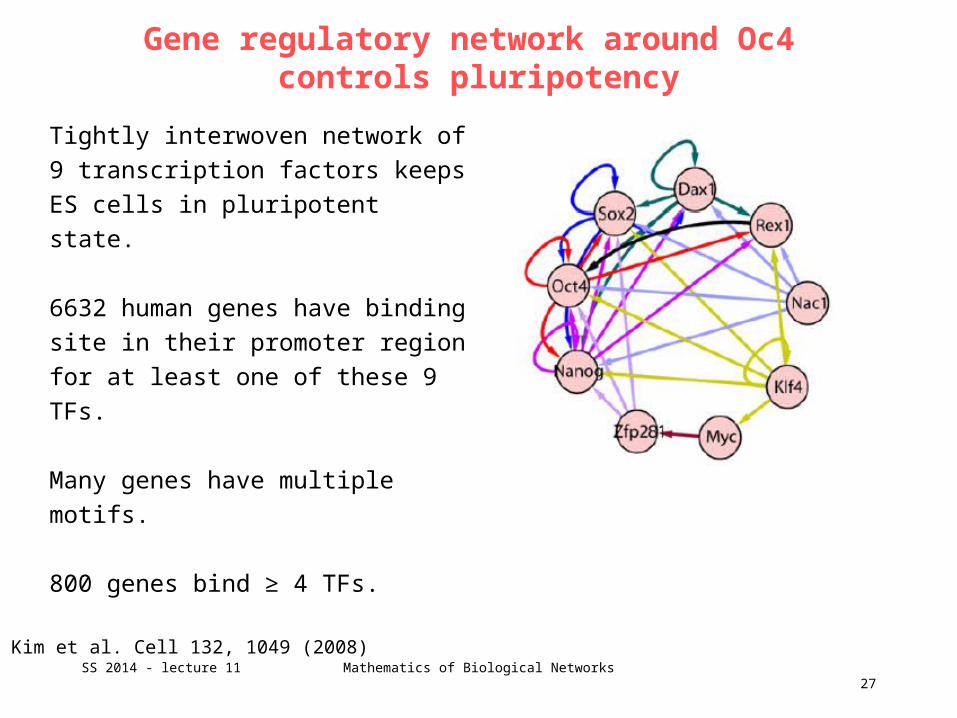
Gene regulatory network around Oc4 controls pluripotency
Tightly interwoven network of 9
transcription factors keeps ES cells in
pluripotent state.
6632 human genes have binding site in
their promoter region for at least one of
these 9 TFs.
Many genes have multiple motifs.
800 genes bind ≥ 4 TFs.
Kim et al. Cell 132, 1049 (2008)SS 2014 - lecture 11 Mathematics of Biological Networks
28
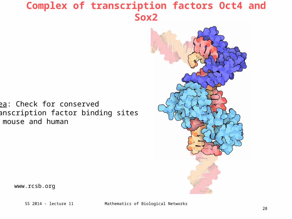
Complex of transcription factors Oct4 and Sox2
www.rcsb.org
Idea: Check for conservedtranscription factor binding sites in mouse and human
SS 2014 - lecture 11 Mathematics of Biological Networks
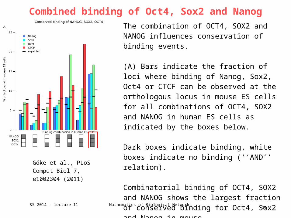
Combined binding of Oct4, Sox2 and Nanog
29SS 2014 - lecture 11 Mathematics of Biological Networks
Göke et al., PLoS
Comput Biol 7,
e1002304 (2011)
The combination of OCT4, SOX2 and NANOG influences conservation of binding events. (A) Bars indicate the fraction of loci where binding of Nanog, Sox2, Oct4 or CTCF can be observed at the orthologous locus in mouse ES cells for all combinations of OCT4, SOX2 and NANOG in human ES cells as indicated by the boxes below.
Dark boxes indicate binding, white boxes indicate no binding (‘‘AND’’ relation).
Combinatorial binding of OCT4, SOX2 and NANOG shows the largest fraction of conserved binding for Oct4, Sox2 and Nanog in mouse.

Increased Binding conservation in ES cells at developmental enhancers
Göke et al., PLoS
Comput Biol 7,
e1002304 (2011)
Fraction of loci where binding of Nanog, Sox2, Oct4 and CTCF can be observed at the orthologous locus in mouse ESC.
Combinations of OCT4, SOX2 and NANOG in human ES cells are discriminated by developmental activity as indicated by the boxes below. Dark boxes : ‘‘AND’’ relation, light grey boxes with ‘‘v’’ : ‘‘OR’’ relation, ‘‘?’’ : no restriction. Combinatorial binding events at develop-mentally active enhancers show the highest levels of binding conservation between mouse and human ES cells.
30SS 2014 - lecture 11 Mathematics of Biological Networks
31
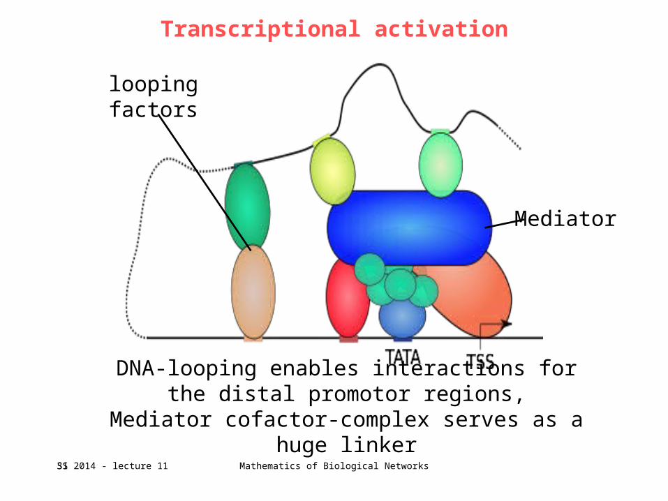
Transcriptional activation
Mediator
looping factors
DNA-looping enables interactions for the distal promotor regions,
Mediator cofactor-complex serves as a huge linker
SS 2014 - lecture 11 Mathematics of Biological Networks

32
cis-regulatory modules
TFs are not dedicated activators or respressors!
It‘s the assembly that is crucial.
coactivators
corepressor
TFs
IFN-enhanceosome from
RCSB Protein Data Bank, 2010
SS 2014 - lecture 11 Mathematics of Biological Networks

Aim: identify Protein complexes involving transcription factors
33
Borrow idea from ClusterOne method:
Identify candidates of TF complexes
in protein-protein interaction graph
by optimizing the cohesiveness
Thorsten Will,Master thesis(accepted for ECCB 2014)SS 2014 - lecture 11 Mathematics of Biological Networks

DDI model
34
domain interactions can reveal which proteins can bind simultaneously if interactions per domain are restricted
transition to domain-domain interactions
“protein-level“network
“domain-level“network
Ozawa et al., BMC Bioinformatics, 2010Ma et al., BBAPAP, 2012
SS 2014 - lecture 11 Mathematics of Biological Networks
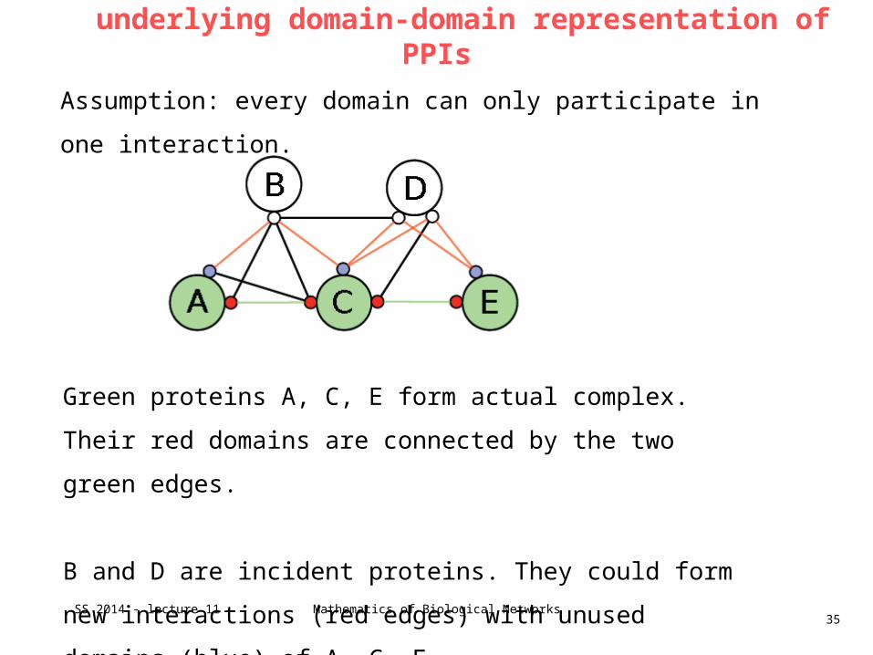
underlying domain-domain representation of PPIs
35
Green proteins A, C, E form actual complex.
Their red domains are connected by the two green edges.
B and D are incident proteins. They could form new interactions
(red edges) with unused domains (blue) of A, C, E
Assumption: every domain can only participate in one interaction.
SS 2014 - lecture 11 Mathematics of Biological Networks
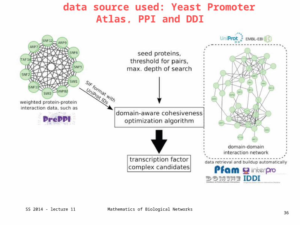
data source used: Yeast Promoter Atlas, PPI and DDI
36SS 2014 - lecture 11 Mathematics of Biological Networks

Daco identifies far more TF complexes than other methods
37SS 2014 - lecture 11 Mathematics of Biological Networks
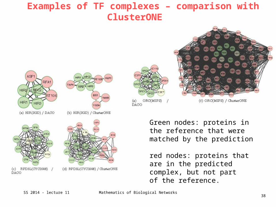
Examples of TF complexes – comparison with ClusterONE
38
Green nodes: proteins in the reference that were matched by the prediction
red nodes: proteins that are in the predicted complex, but not partof the reference.
SS 2014 - lecture 11 Mathematics of Biological Networks

Performance evaluation
39SS 2014 - lecture 11 Mathematics of Biological Networks
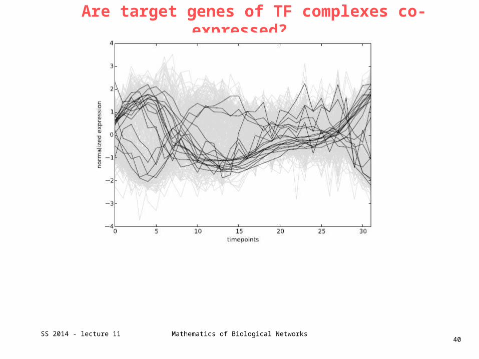
Are target genes of TF complexes co-expressed?
40SS 2014 - lecture 11 Mathematics of Biological Networks

Functional role of TF complexes
41SS 2014 - lecture 11 Mathematics of Biological Networks

42
Complicated regulation of Oct4
Kellner, Kikyo, Histol Histopathol 25, 405 (2010)
SS 2014 - lecture 11 Mathematics of Biological Networks


![V9 series Troubleshooting / Maintenance Manual...V9 Series Reference Manual [1] Explains the functions and operation of the V9 series. 1065NE V9 Series Reference Manual [2] 1066NE](https://static.fdocuments.in/doc/165x107/5fdc0f46901d8161831e54dd/v9-series-troubleshooting-maintenance-v9-series-reference-manual-1-explains.jpg)