UvA-DARE is a service provided by the library of the University of Amsterdam (http://dare.uva.nl)

UvA-DARE (Digital Academic Repository)

Holographic entanglement entropy and gravitational anomalies

Castro Anich, A.; Detournay, S.; Iqbal, N.; Perlmutter, E.

Published in:The Journal of High Energy Physics

DOI:10.1007/JHEP07(2014)114

Link to publication

Citation for published version (APA):Castro, A., Detournay, S., Iqbal, N., & Perlmutter, E. (2014). Holographic entanglement entropy and gravitationalanomalies. The Journal of High Energy Physics, 2014(7), [114]. DOI: 10.1007/JHEP07(2014)114

General rightsIt is not permitted to download or to forward/distribute the text or part of it without the consent of the author(s) and/or copyright holder(s),other than for strictly personal, individual use, unless the work is under an open content license (like Creative Commons).

Disclaimer/Complaints regulationsIf you believe that digital publication of certain material infringes any of your rights or (privacy) interests, please let the Library know, statingyour reasons. In case of a legitimate complaint, the Library will make the material inaccessible and/or remove it from the website. Please Askthe Library: http://uba.uva.nl/en/contact, or a letter to: Library of the University of Amsterdam, Secretariat, Singel 425, 1012 WP Amsterdam,The Netherlands. You will be contacted as soon as possible.

Download date: 02 Dec 2018

JHEP07(2014)114

Published for SISSA by Springer

Received: June 22, 2014

Accepted: July 5, 2014

Published: July 23, 2014

Holographic entanglement entropy and gravitational

anomalies

Alejandra Castro,a Stephane Detournay,b Nabil Iqbalc and Eric Perlmutterd

aInstitute for Theoretical Physics, University of Amsterdam,

Science Park 904, Postbus 94485, 1090 GL Amsterdam, The NetherlandsbPhysique Theorique et Mathematique,

Universite Libre de Bruxelles and International Solvay Institutes,

Campus Plaine C.P. 231, B-1050 Bruxelles, BelgiumcKavli Institute for Theoretical Physics, University of California,

Santa Barbara CA 93106, U.S.A.dDAMTP, Centre for Mathematical Sciences, University of Cambridge,

Cambridge, CB3 0WA, U.K.

E-mail: acastro@uva.nl, sdetourn@ulb.ac.be, niqbal@kitp.ucsb.edu,

E.Perlmutter@damtp.cam.ac.uk

Abstract: We study entanglement entropy in two-dimensional conformal field theories

with a gravitational anomaly. In theories with gravity duals, this anomaly is holographically

represented by a gravitational Chern-Simons term in the bulk action. We show that the

anomaly broadens the Ryu-Takayanagi minimal worldline into a ribbon, and that the

anomalous contribution to the CFT entanglement entropy is given by the twist in this

ribbon. The entanglement functional may also be interpreted as the worldline action for

a spinning particle — that is, an anyon — in three-dimensional curved spacetime. We

demonstrate that the minimization of this action results in the Mathisson-Papapetrou-

Dixon equations of motion for a spinning particle in three dimensions. We work out several

simple examples and demonstrate agreement with CFT calculations.

Keywords: AdS-CFT Correspondence, Anomalies in Field and String Theories

ArXiv ePrint: 1405.2792

Open Access, c© The Authors.

Article funded by SCOAP3.doi:10.1007/JHEP07(2014)114

JHEP07(2014)114

Contents

1 Introduction 1

2 Quantum entanglement in 2d CFTs with gravitational anomalies 3

2.1 Gravitational anomalies 3

2.2 Renyi and entanglement entropy in the presence of a gravitational anomaly 5

2.3 Applications 7

2.3.1 Ground state 7

2.3.2 Ground state, boosted interval 7

2.3.3 Finite temperature and angular potential 8

2.3.4 Holographic CFTs at large central charge 9

3 Holographic entanglement entropy in topologically massive gravity 10

3.1 Gravitational Chern-Simons term 10

3.2 Holographic entanglement entropy: Coney Island 13

3.3 Spinning particles from an action principle 17

4 Applications 19

4.1 Poincare AdS 21

4.2 Poincare AdS, boosted interval 22

4.3 Rotating BTZ black hole 23

4.4 Thermal entropies 24

5 Discussion 25

A Conventions 28

B Details of cone action 29

C Details of variation of probe action 30

D Details of backreaction of spinning particle 33

E Chern Simons formulation of TMG 38

1 Introduction

Holography relates gravitational physics to the dynamics of quantum field theories with a

large number of degrees of freedom. The precise mechanism governing the emergence of

an effective geometry from field-theoretical degrees of freedom remains somewhat unclear.

However, recent work has shown that the concept of quantum entanglement is likely to

– 1 –

JHEP07(2014)114

play a key role in an eventual understanding of this emergence. Consider the entanglement

entropy of a spatial region X in the quantum field theory, defined as the von Neumann

entropy of the reduced density matrix ρX characterizing the spatial region. This is a

very complicated and nonlocal observable. However, in field theories with semiclassical

gravity duals governed by Einstein gravity, there exists a simple and elegant formula for

the entanglement entropy, due to Ryu and Takayanagi [1]:

SEE =Amin

4GN, (1.1)

where Amin denotes the area of the bulk minimal surface anchored on the boundary of the

spatial region X. This equation relates two very primitive ideas on either side of the duality

— geometry and entanglement — and thus may provide insight into the reorganization of

degrees of freedom implied by holography.

In this paper we study holographic entanglement entropy in a different class of theories,

namely, two-dimensional conformal field theories with gravitational anomalies [2]. These

theories suffer from a breakdown of stress-energy conservation at the quantum level: this

may be understood as a sensitivity of the theory to the coordinate system used to describe

the manifold on which it is placed. The anomaly is present in any theory with unequal left

and right central charges appearing in the local conformal algebras. If such a theory admits

a gravity dual, the holographic three-dimensional bulk action will contain a gravitational

Chern-Simons term.

We have two main motivations in mind for studying entanglement entropy in such theo-

ries: from a field-theoretical point of view, we would like to better understand the interplay

between anomalies and entanglement entropy. Indeed the celebrated formula SEE = c3 log R

ε

for the entanglement entropy of an interval in the vacuum of a two-dimensional conformal

field theory is an example of a precise relation between these two concepts, but is con-

trolled by the conformal anomaly instead. Another motivation is holographic: as we will

see, in theories with anomalies, entanglement entropy probes other aspects of the dual

bulk geometry.

We find that the sensitivity of the field theory to its coordinate system manifests itself

holographically in an elegantly geometric way: it gives physical meaning to a normal frame

attached to the Ryu-Takayanagi worldine, essentially broadening the minimal worldline

into a ribbon. The anomalous contribution to the entanglement entropy is now given by

the twist in this ribbon:

Sanom =1

4G3µ

∫Cds (n · ∇n) , (1.2)

where C is a curve in the three dimensional bulk and the vectors n and n define a normal

frame to this curve. µ−1 appears in the coefficient of the gravitational Chern-Simons term,

and measures the anomaly coefficient in the dual two-dimensional theory.

Interestingly, just as a the length of a bulk spatial geodesic may be understood as the

action of a massive point particle propagating in the bulk, this new term may be under-

stood in terms of the action of a spinning particle, i.e. an anyon in AdS. Boundary intuition

for this result comes from the fact that in two-dimensional conformal field theories with

– 2 –

JHEP07(2014)114

a gravitational anomaly, the twist fields used to compute entanglement entropy acquire

nonzero spin proportional to the anomaly coefficient. We discuss the bulk interpretation

of this action in detail, demonstrating in particular that its variation results in the usual

Mathisson-Papapetrou-Dixon equations of motion for a spinning particle in general relativ-

ity [3–5]. Thus our results may also be viewed as the construction of the worldline action

of an anyon in curved space. We anticipate further applications of this formalism.

A brief outline of the paper follows. In section 2 we use two-dimensional conformal

field theory techniques to study Renyi and entanglement entropy in field theories with

gravitational anomalies; no use is made of holographic duality in that section. In section 3

we derive the bulk result (1.2) by a careful evaluation of the action of a cone in topologically

massive gravity, following techniques developed in [6]. We also discuss its interpretation in

terms of the action of a spinning particle and the relation to the Mathisson-Papapetrou-

Dixon equations. In section 4 we apply (1.2) to various simple spacetimes of interest,

holographically deriving results that agree with the field theory calculations from section 2.

We conclude with a brief discussion and summary of future directions in section 5. Many

important details of the derivations have been relegated to various appendices.

Appendix E presents a very different reformulation of the results of this paper, using

the approach studied in [7] to instead compute entanglement entropy from bulk Wilson

lines in the Chern-Simons formulation of topologically massive gravity.

Previous discussion of entanglement entropy in topologically massive gravity in-

cludes [8, 9]: we believe that these works are incomplete in that they do not deal sufficiently

carefully with the subtle lack of diffeomorphism invariance expected in these theories.

2 Quantum entanglement in 2d CFTs with gravitational anomalies

2.1 Gravitational anomalies

We begin by recalling some basics about gravitational anomalies in 2d conformal field

theories (CFTs). More complete accounts of the subject, including generalization to higher

dimensions, can be found in e.g. [2, 10, 11].

A 2d CFT has Virasoro symmetries on the left and right that are generated by

holomorphic and anti-holomorphic components of the stress tensor, T (z) ≡ 2πTzz and

T (z) ≡ 2πTzz, respectively. The algebras take the familiar forms

T (z)T (0) ∼ cL/2

z4+T (0)

z2+∂T (0)

z+ . . . ,

T (z)T (0) ∼ cR/2

z4 +T (0)

z2 +∂T (0)

z+ . . . . (2.1)

Associated to each algebra is an independent central charge. EL and ER will denote the

left and right Virasoro zero modes, respectively.

One can couple any QFT to a background metric gij which acts as a source for the

stress tensor Tij , where (i, j) run over the spacetime coordinates (z, z). In terms of the

QFT generating functional W = − logZ, the stress tensor is defined as

Tij =2√g

δW

δgij. (2.2)

– 3 –

JHEP07(2014)114

If cL 6= cR in a 2d CFT, one cannot consistently promote the background metric to a

dynamical field: that is, the CFT suffers from a gravitational anomaly. Examples include

theories with chiral matter and holomorphic CFTs [12, 13].

The anomaly so defined can be presented in two ways. On the one hand, it is man-

ifest as a diffeomorphism anomaly, in which case the stress tensor is symmetric but not

conserved. Under an infinitesimal diffeomorphism generated by ξi, the metric transforms as

δgij = ∇(iξj) . (2.3)

Non-invariance of the CFT generating functional implies

∇iTij =

(cL − cR

96π

)εkl∂k∂mΓmjl . (2.4)

On the other hand, the anomaly can appear as a Lorentz anomaly — that is, an anomaly

under local frame rotations — in which case the stress tensor is conserved but not sym-

metric. Working in the tangent frame, we have the vielbein eai, spin connection ωab,i and

curvature 2-form Rab, where (a, b) are frame indices; see [10] for a fuller description of the

passage between metric and frame formulations. Under an infinitesimal frame rotation,

the vielbein transforms as

δeai = −αabebi (2.5)

with αab = −αba the rotation parameter. Non-invariance of the CFT generating functional

implies that this stress tensor, call it Tij , obeys

Tab − Tba =

(cL − cR

48π

)?Rab , (2.6)

where ?Rab is the Hodge star of the curvature 2-form,

Rab =1

2Rijkle

ia e

jb dx

k ∧ dxl . (2.7)

The presentation of the anomaly is a matter of choice: shifting from one to the other can

be done by adding a local counterterm to the CFT generating functional [14, 15].1

The anomaly presented thus far is the so-called “consistent” form, obtained from a

generating functional that satisfies the Wess-Zumino consistency conditions. There exists

a “covariant” form of the anomaly, in which covariance of the stress tensor is restored via

improvement terms,

Tij = Tij + Yij (2.8)

for suitably chosen Yij (the “Bardeen-Zumino polynomials”) [15]. The covariant cur-

rents (2.8) can be derived from a modified generating functional living in 2+1 dimen-

sions. Framed as a diffeomorphism anomaly, for instance, the non-conservation equation

in covariant form becomes

∇iTij =

(cL − cR

96π

)εkj∂kR , (2.9)

1This is succinctly captured in the language of the anomaly polynomial. For a gravitational anomaly in

a 2d CFT, the polynomial is P4(R) = Tr(R ∧R) = dω3. The choice of diffeomorphism or Lorentz anomaly

corresponds to the choice of whether to express the curvature as R = dΓ + Γ ∧ Γ or R = dω + ω ∧ ω,

respectively.

– 4 –

JHEP07(2014)114

where R = Rijgij is the Ricci scalar; note the absence of explicit factors of Γ. In a

holographic context, the usual AdS/CFT dictionary identifying boundary data with sources

in the CFT generating functional naturally leads to the consistent form [16].

2.2 Renyi and entanglement entropy in the presence of a gravitational

anomaly

Consider a QFT living on some Riemannian manifold M , in a state defined by some given

density matrix. One can form a reduced density matrix, ρ, by tracing out degrees of

freedom exterior to some spatial region at fixed Euclidean time. The Renyi entropy Sn is

defined as

Sn =1

1− nlog Trρn , (2.10)

where n is a positive integer. In a 2d QFT, the spatial region is the union of N ∈ Z disjoint

intervals. Upon analytically continuing n to positive real values, one can take the limit

n→ 1 to obtain the entanglement, or von Neumann, entropy,

SEE = limn→1

Sn = −Tr ρ log ρ . (2.11)

This procedure involves ambiguities in principle; we will employ the naive analytic con-

tinuation, based on precedent in similar 2d CFT entanglement calculations. For further

details on this construction, we direct the reader to [17–19].

Computing entanglement entropy via the replica trick amounts to computing the Renyi

entropy for arbitrary n. The latter is equivalent to computing a QFT partition function

Zn on a branched cover of M , with branch cuts along the entangling surface. The precise

relation is

Trρn =Zn

(Z1)n. (2.12)

This technique is applicable in any state that can be defined using a functional inte-

gral. Alternatively, one can eschew this topological perspective, and instead compute

Trρn as a correlation function on M of twist operators inserted at the boundary of the

entangling region.

We focus on 2d CFTs henceforth, calling a generic CFT C. The branched covers

of M are Riemann surfaces of N - and n-dependent genus; when M = C, for example,

g = (N−1)(n−1). Rather than computing partition functions on arbitrary genus Riemann

surfaces directly, we will employ the twist field perspective [17, 20]. For N spatial intervals

bounded by endpoints ui, vi, one inserts N twist operators Φ+ at the endpoints ui and

N twist operators Φ− at the endpoints vi, and computes their 2N -point correlator on M :

Tr ρn =

⟨N∏i=1

Φ+(ui)Φ−(vi)

⟩Cn/Zn

. (2.13)

As the subscript denotes, the correlator is evaluated in the orbifold theory Cn/Zn. Φ+

and Φ− act oppositely with respect to the cyclic permutation symmetry Zn, and have a

nontrivial OPE. The n-dependence also enters (2.13) through the scaling dimensions of the

twist operators, to be derived momentarily.

– 5 –

JHEP07(2014)114

For a CFT with cL 6= cR, these techniques still apply. The presence of a gravitational

anomaly does not spoil the use of functional integrals; one need only be careful about their

transformation properties. This brings us to the central novelty: in a CFT with cL 6= cR,

the twist fields Φ± have nonzero spin controlled by the anomaly coefficient: s ∝ cL − cR.

To derive this fact, following the original method of [17], it is sufficient to consider a

single interval in the ground state of a CFT C, with endpoints (u, v). Before replication, Clives on the complex plane, M = C. The replica surface — call it Rn,1 — has genus zero

for all n, and can be conformally mapped back to the complex plane. If w is a complex

coordinate on Rn,1, then

z =

(w − uw − v

)1/n

, (2.14)

maps Rn,1 7→ C, coordinatized by z. To compute the scaling weights of the twist operators,

consider the one-point functions of the CFT stress tensor components, 〈T (w)〉Rn,1 and

〈T (w)〉Rn,1 . On one hand, one can compute the conformal transformation of the stress

tensor under the map (2.14). On the other, these expectation values can be traded for

correlation functions with twist operators in the orbifold theory, by definition of the twist

operators themselves. Recalling that 〈T (z)〉C = 〈T (z)〉C = 0, one finds

〈T (w)Φ+(u, u)Φ−(v, v)〉Cn/Zn〈Φ+(u, u)Φ−(v, v)〉Cn/Zn

=cL24

(n− 1

n

)(u− v

(w − u)(w − v)

)2

,

〈T (w)Φ+(u, u)Φ−(v, v)〉Cn/Zn〈Φ+(u, u)Φ−(v, v)〉Cn/Zn

=cR24

(n− 1

n

)(u− v

(w − u)(w − v)

)2

. (2.15)

These equations are nothing but the conformal Ward identities for the holomorphic

and anti-holomorphic stress tensors, acting on Virasoro primary operators with scaling

dimensions

hL =cL24

(n− 1

n

), hR =

cR24

(n− 1

n

). (2.16)

Defining conformal dimension ∆ = hL+hR and spin s = hL−hR, we find spinning, anyonic

twist fields as advertised:

∆ =cL + cR

24

(n− 1

n

), s =

cL − cR24

(n− 1

n

). (2.17)

This derivation is a simple extension of the case cL = cR treated in [17] and elsewhere; the

key point is that the calculation holomorphically factorizes.

By deriving twist operator quantum numbers from the CFT stress tensor, this method

fully accounts for the dependence of Renyi and entanglement entropy on the gravitational

anomaly. We are implicitly working with the consistent form of the anomaly, because T (z)

and T (z) are defined through variations of the original CFT generating functional. Notice

that in computing entanglement entropy as the n → 1 limit of Renyi entropy, the twist

operators are analytically continued from anyons to spinless bosons. However, the ratio

s/∆ is independent of n.

– 6 –

JHEP07(2014)114

2.3 Applications

With these results in hand we proceed to easily derive universal results for single interval

Renyi and entanglement entropy in 2d CFTs with arbitrary (cL, cR). From (2.13), this

merely involves computing the two-point function of Φ+ and Φ−. For a CFT in its ground

state, on a circle, or at finite temperature and angular potential, the functional form of

the correlator is fixed by conformal symmetry [21]. We will also comment on more general

entanglement entropies in holographic CFTs with cL 6= cR.

We work with an interval [0, R] in a CFT on a line, with R ∈ R, unless otherwise

noted. Thus, we wish to compute

Sn =1

1− nlog〈Φ+(R)Φ−(0)〉Cn/Zn . (2.18)

We will reinstate the UV cutoff as needed for dimensional analysis.

2.3.1 Ground state

In this case, M = C, so (2.17) and (2.18) yield

Sn =

(1 +

1

n

)cL + cR

12log

(R

ε

). (2.19)

and the entanglement entropy is easily obtained,

SEE =cL + cR

6log

(R

ε

). (2.20)

This was first derived in [22]. The anomaly makes no contribution to (2.20). For holo-

graphic CFTs, this state is dual to Poincare AdS.

2.3.2 Ground state, boosted interval

Now consider a complex interval [0, z], with z ∈ C somewhere off the real axis. We find

Sn =

(1 +

1

n

)(cL12

log

(z

ε

)+cR12

log

(z

ε

)). (2.21)

In this case, we do see a contribution from the anomaly. If we define z = Reiθ, we find an

entanglement entropy

SEE =cL + cR

6log

(R

ε

)+cL − cR

6iθ . (2.22)

This setup is just a rotation of the previous one, but in a theory with a Lorentz anomaly,

observables are sensitive to the choice of frame. Equivalently, in the language of the

diffeomorphism anomaly, observables are sensitive to the choice of coordinates used to

define a constant time slice.

As (2.22) shows, in the absence of Euclidean time reflection symmetry (z ↔ z) a

Euclidean CFT partition function need not be real.2 This is familiar from the thermal

2In fact, the anomalous piece had to be purely imaginary on general grounds. Thinking of Tr ρn as a

CFT partition function on a Riemann surface, as in (2.12), we note that only the imaginary part of logZ

can ever receive an anomalous contribution. Thus, the frame rotation to a complex interval must lead to

an imaginary piece of the Euclidean Renyi entropy.

– 7 –

JHEP07(2014)114

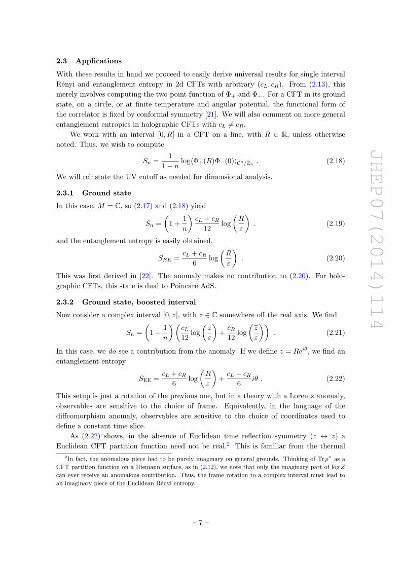
Figure 1. Flow of entanglement through boosted interval.

partition function of a non-anomalous CFT at finite temperature and chemical potential for

angular momentum. As in that case, the complexity of (2.22) is consistent with a sensible,

real Lorentzian interpretation: under the analytic continuation z = x − t, z = x + t, the

angle θ maps to a boost parameter κ as θ = iκ. Plugging this into (2.22) yields a real

contribution to the entanglement entropy due to an anomalous Lorentz boost:

SEE =cL + cR

6log

(R

ε

)− cL − cR

6κ . (2.23)

There is a simple physical argument for this due to Wall [23], as shown in figure 1.

To understand figure 1, suppose that we have quantized our theory with respect to the

time coordinate t; thus we understand how to compute entanglement entropy on the slice

t = 0. Consider now the entanglement through the boosted interval (ending at R′). We

would like to relate this to entanglement computed at t = 0. We see that at t = 0 all the

left-movers that will eventually pass through the boosted interval are inside RL, whereas

all the right-movers are inside RR. Assuming factorization of left and right-movers, the

entanglement computed at t = 0 then should be

SEE =cL6

log

(RLε

)+cR6

log

(RRε

)(2.24)

If the hyperbolic boost angle is κ, then RL = Re−κ and RR = Reκ: this immediately

reproduces (2.23).

2.3.3 Finite temperature and angular potential

Consider now a spatial interval [0, R] in a general Lorentzian CFT on a line at finite

temperature, T = β−1, and chemical potential for angular momentum, Ω. The CFT now

lives on a cylinder with a compact thermal cycle, M = S1×R. For a holographic CFT, this

state is dual to the rotating, planar BTZ black hole. After Wick rotation, the Euclidean

partition function is

Z = Tr(e−βH−βΩEJ) (2.25)

where

H = ER + EL −cL + cR

24, J = ER − EL +

cL − cR24

, (2.26)

– 8 –

JHEP07(2014)114

and we define ΩE to be real via the standard analytic continuation Ω = iΩE . It is convenient

to define left and right temperatures, TL 6= TR; the respective inverse temperatures (βL, βR)

are defined in terms of (β,ΩE) as

βL = β(1 + iΩE) , βR = β(1− iΩE) . (2.27)

Notice that in the ground state on the cylinder, EL = ER = 0, there is a nonzero “Casimir

momentum” J0 in addition to the usual ground state energy, E0:

E0 = −cL + cR24

, J0 =cL − cR

24. (2.28)

This effect stems from the imbalanced chiral contributions to the Casimir energy.

To compute the Renyi entropy, we plug the universal form of cylinder correlation

functions into (2.18), which yields

Sn =

(1 +

1

n

)[cL12

log

(βLπε

sinhπR

βL

)+cR12

log

(βRπε

sinhπR

βR

)], (2.29)

and in the limit n→ 1,

SEE =cL6

log

(βLπε

sinhπR

βL

)+cR6

log

(βRπε

sinhπR

βR

). (2.30)

For βL 6= βR, there is an anomalous contribution that maps to a real entanglement entropy

in Lorentzian signature. The formula neatly factorizes, and yields the correct Cardy entropy

in the thermal limit R (βL, βR). In analogy to the case of the complex interval on the

plane, we can think of ΩE as a boost parameter, or as parameterizing passage to a rotating

frame.

From the above results, we can also compute entanglement for a CFT at zero tem-

perature on a cylinder of size L. We can read off the Renyi and entanglement entropies

from (2.29)–(2.30) by simply taking βL = βR 7→ −iL. This case sees no anomalous contri-

bution. For holographic CFTs, this state is dual to global AdS.

2.3.4 Holographic CFTs at large central charge

The results in this section universally apply to all CFTs with arbitrary (cL, cR). For this

(sub)subsection, we specialize to a class of “holographic” CFTs at large total central charge

cL+cR: this should be understood as the class of CFTs which are likely to have semiclassical

gravity duals, although no use will be made of holography in this section. A constructive

definition of such CFTs was given in [19, 24]: aside from fundamental properties of unitarity,

modular invariance and compactness, their essential property is that the OPE coefficients

and density of states with ∆ . cL + cR do not scale exponentially with large cL + cR.

In anticipation of our study of holographic entanglement in TMG, this is an eminently

relevant class of theories to consider.

Recent work [19, 24–30] has shown that in such large central charge 2d CFTs with

or without gravitational anomalies, Renyi and entanglement entropies can be derived for

otherwise non-universal cases, involving higher genus manifolds M or multiple intervals

– 9 –

JHEP07(2014)114

N > 1. For example, one can think of (2.30) as the high temperature limit of entanglement

entropy of a single interval on a torus, M = T 2, with complex modular parameter τ =

iβL/2π. Torus two-point correlators are non-universal. For a CFT satisfying the above

properties, however, the entanglement entropy of a single interval on the torus has been

argued to be given by (2.30) for all temperatures above the Hawking-Page transition at

leading order in large cL + cR [26, 28], provided that the size of the interval is smaller than

half of the circle.3 This provides a modest consistency check of (2.30).

As a second example, consider the Renyi and entanglement entropy of multiple inter-

vals in the ground state. As 2N -point twist correlators with N > 1, these are non-universal

in general, but can be computed systematically in holographic CFTs in a large cL + cRexpansion [19, 24, 27, 28, 30]. This is true regardless of whether the CFT suffers from

a gravitational anomaly. At leading order in large cL + cR, the ground state entangle-

ment entropy is simply a sum over single interval contributions (2.20) subject to a certain

minimization prescription [24]:

SEE =cL + cR

6min

∑(i,j)

log

(zi − zjε

), (2.31)

where zi label the endpoints, i = 1, . . . , 2N .

3 Holographic entanglement entropy in topologically massive gravity

We turn now to the holographic description of theories with gravitational anomalies. As

mentioned earlier, the bulk action describing such a theory has a gravitational Chern-

Simons term in its action. In trying to understand the anomalous contribution to entan-

glement, it is sufficient to work with topologically massive gravity (TMG), which couples

the Chern-Simons term to ordinary Einstein gravity. The Ryu-Takayanagi prescription for

computing entanglement entropy will require modification in this case. Roughly speaking,

just as in ordinary 3d gravity the Ryu-Takayanagi worldline can be viewed as the trajec-

tory traced out by a heavy bulk particle, we will show that in TMG the analog of this idea

involves a massive spinning particle, whose on-shell action yields the holographic entangle-

ment entropy. This is nothing but the extension of the twist field spin into the bulk. Thus,

our task is to construct an action for such a particle and understand its dynamics. As we

will see, our action makes satisfying contact with previous literature on spinning particles

in general relativity.

We begin this section by briefly recalling some salient features of TMG.

3.1 Gravitational Chern-Simons term

The original work on TMG dates back to [32–34]; for a more modern treatment see e.g. [16,

35, 36]. The action is the sum of the Einstein-Hilbert term and a gravitational Chern-

3For larger interval sizes there may be a competing saddle, holographically manifest as the disconnected

surface contributing to the Ryu-Takayanagi formula, i.e. the “entanglement plateaux” of [31].

– 10 –

JHEP07(2014)114

Simons term:

STMG =1

16πG3

∫d3x√−g(R+

2

`2

)+

1

32πG3µ

∫d3x√−gελµνΓρλσ

(∂µΓσρν +

2

3ΓσµτΓτνρ

), (3.1)

where we have included a negative cosmological constant. µ is a real coupling with dimen-

sions of mass. Even though the action has explicit dependence on Christoffel symbols, the

equations of motion are covariant: explicitly, they are

Rµν −1

2gµνR−

1

`2gµν = − 1

µCµν , (3.2)

where Cµν is the Cotton tensor,

Cµν = ε αβµ ∇α(Rβν −

1

4gβνR

). (3.3)

The Cotton tensor is symmetric, transverse and traceless,

εαµνCµν = ∇µCµν = Cµµ = 0 . (3.4)

Consequently, all solutions of TMG have constant scalar curvature, R = −6/`2, and the

equations of motion can be written as

Rµν +2

`2gµν = − 1

µCµν . (3.5)

The Cotton tensor thus measures deviations from an Einstein metric.

It is clear from (3.3)–(3.5) that TMG admits all solutions of pure three dimensional

gravity, namely, Einstein metrics for which Cµν = 0. The theory also admits a wide class

of non-Einstein metrics which are not locally AdS3. We briefly note that TMG can also be

cast in a Chern-Simons formulation; in appendix E we review that approach to the theory.

Many unusual properties of TMG are put into sharper focus in a holographic con-

text. This theory has been extensively studied in the context of AdS3/CFT2 by [16, 37–

39], among many other authors.4 Specializing for the moment to locally AdS3 solutions,

the application of Brown-Henneaux [43] for TMG shows that the classical phase space of

asymptotically AdS3 backgrounds is organized in two copies of the Virasoro algebra with

central charges

cL =3`

2G3

(1− 1

µ`

), cR =

3`

2G3

(1 +

1

µ`

). (3.6)

As detailed in the previous section, the unequal central charges indicate the presence of

a gravitational anomaly in the dual CFT. This is consistent with the transformation of

the gravitational Chern-Simons term under bulk diffeomorphisms: in particular, the bulk

action is invariant up to a boundary term that captures the nonzero divergence of the CFT

4Holography for TMG has been also the cradle of some controversy at µ = 1, the so-called “chiral point,”

which we will not discuss here. See e.g. [40–42] and references within.

– 11 –

JHEP07(2014)114

stress tensor in (2.4) [38]. This is the usual elegant mechanism of holographic anomaly

generation in AdS/CFT [44] as applied to a gravitational anomaly.

One can also perform a precise matching of thermodynamic observables of the bulk

and boundary theories. The presence of the gravitational Chern-Simons term generically

affects the observables in the bulk, even for locally AdS3 solutions. One intriguing example

is the introduction of nonzero angular momentum into global AdS3: the ADM charges are

`MAdS = − `

8G3= −cL + cR

24, JAdS = − 1

8G3µ=cL − cR

24, (3.7)

which match the CFT result (2.28) for ground state energy and Casimir momentum on

the cylinder [38]. At finite temperature, the bulk admits BTZ black holes, which are dual

to thermal states in the CFT. The asymptotic density of states of the CFT is governed by

the Cardy formula [45],

S = 2π

√cLEL

6+ 2π

√cRER

6. (3.8)

Happily, this has been shown to equal the Wald entropy of BTZ black holes in TMG or

any covariant higher derivative modification thereof [37, 46–50].

The novel solutions of TMG are those with Cµν 6= 0, which are not locally AdS3.

An interesting subset of such solutions, denoted “warped AdS3”, were constructed in [51–

53], along with warped black hole counterparts. Viewed holographically, the main fea-

ture of asymptotically warped AdS3 geometries is that they do not obey Brown-Henneaux

boundary conditions, so (3.6) is not applicable; indeed, the nature and symmetries of a

putative holographic dual CFT are not very well understood (see, e.g., [54–58] and refer-

ences within).

In the following sections, we will deal with the Euclidean theory for both technical and

conceptual reasons. The gravitational Chern-Simons term is a parity odd term under time

reversal, hence a Wick rotation t→ tE = it yields

SEuc =1

16πG3

∫d3x√g

(R+

2

`2

)+

i

32πG3µ

∫d3x√gελµνΓρλσ

(∂µΓσρν +

2

3ΓσµτΓτνρ

), (3.9)

and the equations of motion are

Rµν +2

`2gµν = − i

µCµν . (3.10)

The appearance of the factor of i in (3.10) is important: for a real metric, the left and right

hand side of (3.10) must vanish independently, hence restricting the space of real solutions

to the Einstein metrics of pure gravity. Our presentation of the holographic entanglement

functional for TMG relies only on general properties of the theory, modulo some mild

assumptions; nevertheless, it is not completely obvious how to apply our result to the full

set of solutions of TMG, for which the Euclidean continuation is unclear. We will comment

on these subtleties in the Discussion section.

– 12 –

JHEP07(2014)114

3.2 Holographic entanglement entropy: Coney Island

We now want to understand how the computation of holographic entanglement entropy in

TMG reflects the gravitational anomaly of a dual CFT. In principle, there exists a perfectly

well-defined procedure for computing Renyi entropy for any n. In (2.11)–(2.12) we wrote

the entanglement entropy as

SEE = limn→1

1

1− n(logZn − n logZ1) . (3.11)

Using the AdS/CFT dictionary, we interpret Zn as the gravitational partition function for a

3-manifoldMn asymptotic to a replica manifold Rn ≡ ∂Mn at conformal infinity [19, 25].

In the semiclassical limit we can approximate this partition function by computing the

action of Mn.

In [6] an efficient algorithm was developed for computing such actions in states that

admit a description involving a Euclidean partition function. We do not review details

here but just state the result: in the n→ 1 limit, one can understand the action ofMn by

studying the action of a bulk geometry with a conical surplus of 2π(n−1) along a worldline

C extending into the bulk, i.e.

SEE = −∂n(Scone)∣∣n=1

. (3.12)

The Einstein-Hilbert action evaluated on this conical surplus simply measures the proper

length of C. Furthermore one finds that consistency of the bulk equations requires (in the

case of Einstein gravity) that the curve C must be a bulk geodesic, and one eventually finds

S(RT)EE =

Lmin

4G3. (3.13)

This constitutes a proof of the celebrated Ryu-Takayanagi formula (RT) for the entangle-

ment entropy [1, 59, 60], at least for the set of states that can be studied using a Euclidean

partition function.

We would now like to apply these techniques to TMG. The fact that the bulk action

is not quite gauge-invariant will play an interesting role in our analysis: the existence of

this anomaly will effectively introduce new data along the worldline, broadening the usual

Ryu-Takayanagi worldline into a ribbon. As we will demonstrate in detail, this is the bulk

representation of the anomalous contributions to CFT entanglement discussed in section 2,

a statement we will verify in a number of examples.

Consider a regularized cone in three-dimensional Euclidean space with opening angle

2π(1 + ε), so that ε = n− 1. The tip of this cone defines a one-dimensional worldline that

we take to extend along a spacelike direction parametrized by y. We use flat coordinates σa

for the two perpendicular directions, and the tip of the cone is then at σa = 0. A suitable

metric ansatz for this cone is then

ds2 = eεφ(σ)δabdσadσb + (gyy +Kaσ

a + · · ·) dy2 + eεφ(σ)Ua(σ, y)dσady (3.14)

In this parametrization the extrinsic curvatures Ka are Taylor coefficients in the expansion

of gyy in the σa directions, and they measure the deviation of the trajectory from a geodesic.

– 13 –

JHEP07(2014)114

φ(σ) stores the information of the regularization of the cone: importantly, it can be picked

to fall off exponentially outside a small core.

We now compute the action of this cone (3.9) to first order in ε, using standard

techniques [6, 61, 62], although the generalization to TMG requires some care. We present

details of the calculation, including explicit expressions for the regulator function φ(σ), in

appendix B.

Let us recall the logic by first evaluating the Einstein part of the action (3.9). The

Ricci scalar receives contributions of the form ∇2aφ. Evaluating the integrals we find

Scone,Einstein = − ε

4G3

∫Cdy√gyy +O(ε2) . (3.15)

Although this expression was evaluated in the coordinate system given by (3.14), it is clear

that it is simply measuring the proper distance along the cone-tip worldline. In particular,

there is no obstruction to writing a fully covariant expression: parametrizing the cone tip

by Xµ(s), we simply find

Scone,Einstein = − ε

4G3

∫Cds

√gµν(X)XµXν +O(ε2) . (3.16)

We now attempt to repeat this calculation for the gravitational Chern-Simons part

of (3.9). A very similar calculation yields

Scone,CS = − iε

16µG3

∫dy εab∂aUb (3.17)

Obtaining this expression involves an integration by parts. The validity of this procedure

requires a careful understanding of the boundary conditions on the integral, as we discuss

in appendix B.

Now we note that the explicit appearance of the metric functions Ua(y) makes this

expression qualitatively different from (3.15): in writing down the metric (3.14) we actually

implicitly made a coordinate choice about how the transverse plane parametrized by σa

rotates as we move in the y direction. To be more explicit, if we perform an infinitesimal

y-dependent rotation:

δσa = −θ(y)εabσb (3.18)

then the curl of the vector field Ua transforms inhomogenously:

δ(εab∂aUb(y)

)= 4θ′(y) . (3.19)

The Chern-Simons action is not invariant under this coordinate transformation. Instead it

shifts by a boundary term from the endpoints of the y integral:

δScone,CS = − iε

4µG3(θ(yf )− θ(yi)) . (3.20)

This is consistent with general expectations for Chern-Simons terms. However it appears to

make it impossible to construct a local covariant expression analogous to (3.16). To proceed

– 14 –

JHEP07(2014)114

Figure 2. Evolution of normal vectors n1,2 along the curve C.

we will need to introduce an ingredient that knows about the twisting of the coordinate

system as we move along the curve.

To that end, consider choosing a normal vector to the curve n1 (see figure 2). The

choice of this vector fixes the other normal vector n2 via n1 · n2 = 0.5 Still there is a

local SO(2) freedom in this choice: for our purposes, we want these vectors to store the

information of how the local coordinates change along the curve, and so we will define

them with respect to the coordinate choice of the σa, i.e:

n1 :=∂

∂σ1n2 :=

∂

∂σ2(3.21)

To lowest order in ε these vectors have unit norm, and they are both orthogonal to the

tangent vector v =√gyy∂y. With this definition it is possible to write down a local

expression which reduces to (3.17):

Scone,CS = − iε

4µG3

∫Cds n2 · ∇n1 + . . . , (3.22)

where the dots denote subleading terms in (z, z) and ε. The symbol ∇ with no subscript

indicates a covariant derivative along the worldline:

∇V µ :=dV µ

ds+ Γµλρ

dXρ

dsV λ . (3.23)

We emphasize that this expression is evaluated at the tip of the cone, located in these

coordinates at σa = 0. Furthermore only the linear in ε piece of the action (3.22) is

expected to have a local representation along the worldline.6

The functional (3.22) also appears to be covariant, but this is a delicate point, as in this

derivation n1 and n2 were defined in terms of the base coordinate system. Essentially the

5Up to an overall sign related to a choice of handedness.6We briefly mention the history of the term (3.22). In three flat Euclidean dimensions this expression is

known as the torsion of a curve [63]. It is also known from the physics of anyons, where it appears along the

worldline of a massive particle with a coefficient that measures the fractional spin [64]. It is also discussed

in [65] in relation to the framing anomaly in Chern-Simons theory.

– 15 –

JHEP07(2014)114

anomaly has taken a bulk gravitational degree of freedom that used to be pure gauge and

given it life, binding it to the worldline in the form of a normal vector. As we will explore in

detail in the remainder of this paper, these normal vectors are not true dynamical degrees

of freedom, but their existence and the associated subtle non-covariance of this expression

is precisely what is needed to account for the boundary non-covariance associated with a

gravitational anomaly.

Now using the original expression (3.12) and taking the ε derivative, we find the total

entanglement entropy in topologically massive gravity to be

SEE =1

4G3

∫Cds

(√gµνXµXν +

i

µn2 · ∇n1

)E

, (3.24)

where the first term is the usual Ryu-Takayanagi term and the second is the extra contribu-

tion from the Chern-Simons term. The subscript E reminds us that this whole expression

is evaluated in Euclidean signature.

Let us attempt to interpret this expression in Lorentzian signature, with the path

C spacelike. If we try to analytically continue the complex coordinates (z, z) via z =

x − t, z = x + t, then we see from (3.21) that we can obtain two real Lorentzian normal

vectors (n, n) via

n := in1 = ∂t n := n2 = ∂x . (3.25)

We choose a notation that is no longer symmetric with respect to the two normal vectors,

as one of them is now timelike (n) and the other spacelike (n). Expressing (3.24) in terms

of these vectors we now find the following expression for the entanglement entropy:

SEE =1

4G3

∫Cds

(√gµνXµXν +

1

µn · ∇n

)(3.26)

where everything is now evaluated in Lorentzian signature.

This expression is one of the main results of this paper. It is manifestly real. However

unlike the steps leading to (3.24), this analytic continuation cannot in general be justified,

as the σa coordinate system used above is ill-defined away from a vicinity of C: certainly

there is generally no U(1) isometry along which we can continue the bulk spacetime. Rather

the relation between (3.24) and this formula is equivalent to the relation between the

(justified) Ryu-Takayanagi formula for static spacetimes and its (yet unproven) covariant

generalization [66]. Nevertheless, we will use it for the rest of the paper and find physically

sensible results.

Next, we note that this expression should be evaluated on a worldline C. As it turns

out, the correct worldline is determined by extremizing the functional (3.24). As empha-

sized in [61, 62], the justification of this statement is in principle a different question than

the determination of the functional itself. We present two routes to its justification in

appendix D. We show that the consistency of the TMG equations near a spacetime with

a conical defect constrains the worldline of the defect in a way that requires (3.24) to be

extremized, and we show that viewing (3.24) as a source to the TMG equations creates

the desired conical defect. We now move on to discuss the physical content of the resulting

equations of motion.

– 16 –

JHEP07(2014)114

3.3 Spinning particles from an action principle

Let us take a step back and recapitulate what we expect the cone action to describe in

the bulk. As articulated at the start of this section, the action (3.26) should capture the

physics of a heavy particle with mass m and a continuously tunable spin s determined by

the CFT twist operator quantum numbers (2.17): in other words, we expect an anyon in

curved space. In this section we will flesh out this interpretation, and to make it evident

in what follows we write the entanglement functional (3.26) as

SEE =

∫Cds

(m

√gµνXµXν + s n · ∇n

), (3.27)

with m and s real constants.

The variational principle for (3.27) should include variations with respect to both the

particle position Xµ(s) and the normal vectors (n, n). However, our construction requires

that (n, n) remain normal to the curve , and so if we are to vary them then (3.27) must be

supplemented with the following constraint action:

Sconstraints =

∫Cds[λ1n · n+ λ2n · v + λ3n · v + λ4(n2 + 1) + λ5(n2 − 1)

], (3.28)

where the λi are five Lagrange multipliers that guarantee that n and n are normalized,

mutually orthogonal, and perpendicular to the worldline:

n · v = 0 , n · v = 0 , n · n = 0, n2 = −1, n2 = 1 , (3.29)

which also enforce that n is timelike and n is a spacelike vector. These are the constraints

that allow us to write (3.26) in the first place. Here vµ is the velocity vector:

vµ :=dXµ

ds= Xµ . (3.30)

We choose the affine parameter s of this path to be the proper length along the path and

hence we have vµvµ = 1. The total action for the spinning particle is then

Sprobe =

∫Cds

(m

√gµνXµXν + s n · ∇n

)+ Sconstraints . (3.31)

In addition to the particle trajectory Xµ(s), it appears that we now have a dynamical

degree of freedom corresponding to the rotation of the normal frame along the worldline.

Indeed we have three independent components for each of n and n, and five constraints

associated with (3.28), leaving a single degree of freedom. However as it turns out this is

not a true degree of freedom, as the action is only sensitive to its variation up to boundary

terms. To see this, consider the equation of motion arising from variation of Sprobe with

respect to n:

− s∇nµ + λ1nµ + λ2v

µ + 2λ4nµ = 0 . (3.32)

Contracting with nµ, vµ and nµ respectively results in

λ1 = s n · ∇n λ2 = s v · n , 2λ4 = −sn · ∇n . (3.33)

– 17 –

JHEP07(2014)114

The same analysis for δnSprobe = 0 gives

s∇nµ + λ1nµ + λ3v

µ + 2λ5nµ = 0, (3.34)

and again the appropriate contractions yield

λ1 = sn · ∇n λ3 = −s v · ∇n , 2λ5 = −s n · ∇n . (3.35)

Eqs. (3.33) and (3.35) are six equations, of which five may be satisfied by appropriate

choice of the λi. The equation that remains comes from the fact that λ1 appears in both

sets of equations, and is:

n · ∇n = n · ∇n . (3.36)

However this is not a dynamical equation: as −n2 = n2 = 1, both sides of this equation

are identically zero and this is an identity. Thus (n, n) do not have a dynamical equation

of motion: equivalently, Sprobe is insensitive to small variations of the normal frame along

the trajectory, up to boundary terms. As we will see, these boundary terms will be very

important to us.

A more tedious task is to vary (3.31) with respect to Xµ(s); details can be found in

appendix C. This variation, however, is not trivial and gives rise to

∇ [mvµ + vρ∇sµρ] = −1

2vνsρσRµνρσ , (3.37)

where we define the spin tensor sµν to be

sµν = s (nµnν − nµnν) , (3.38)

These equations are known as the Mathisson-Papapetrou-Dixon (MPD) equations, and

describe the motion of spinning particles in classical general relativity [3–5].7 In (2 + 1)

dimensions they follow from the simple and geometric action (3.31).

Next, using (3.29) we see that the spin tensor may be written in terms of the velocity as

sµν = −sεµνλvλ , (3.39)

indicating that the spin tensor is just the volume form perpendicular to the worldline and

does not actually carry any extra degrees of freedom.8 Note also that the normal vectors

themselves have vanished from the equations of motion: they are required only to set up

the action principle.

Thus to compute entanglement entropy in topologically massive gravity we should

solve the MPD equations (3.37) using the values of m and s inherited from (3.26):

m =1

4G3, s =

1

4µG3, (3.41)

and then evaluate the action (3.26) on the resulting solution.

7See as well [67–71] for a more modern treatment and further references.8In higher dimensions such a rewriting is not possible: sµν there actually carries information about the

direction of the particle’s spin. In that case the MPD equations also include a relation for the evolution of

the spin tensor,

∇sαβ + vαvµ∇sβµ − vβvµ∇sαµ = 0 , (3.40)

which is an identity on (3.39).

– 18 –

JHEP07(2014)114

4 Applications

In this section we finally apply our prescription to the actual computation of holographic

entanglement entropy on various backgrounds of interest. We will compare with the CFT

results found in section 2. Recall that the prescription is as follows: the entanglement

functional (3.26) is

SEE =1

4G3

∫Cds

(√gµνXµXν +

1

µn · ∇n

). (4.1)

It should be evaluated on a curve C in spacetime which is found by extremization of the

functional itself, which results in the Mathisson-Papapetrou-Dixon equations (3.37) for the

motion of a spinning particle of mass m and spin s given by (3.41).

We will limit our discussion to spacetimes that are locally AdS3. This greatly simplifies

the analysis, as here the contraction of the Riemann tensor with sµνvρ vanishes.9 The MPD

equations then reduce to

∇[mvµ − sεµνλvν∇vλ

]= 0 , (4.2)

and furthermore, it is clear that a geodesic

∇vµ = 0 , (4.3)

is a solution to (4.2). Evidently anyons moving on maximally symmetric spaces follow

geodesics.10

So all we need to do is evaluate the second term in the action (4.1) on a geodesic. We

call this term Sanom. For this purpose it will be helpful to rewrite the action in terms of a

single normal vector n using nµ = εµνρvνnρ to find

Sanom =1

4G3µ

∫Cds εµνρv

µnν(∇nρ) . (4.4)

We note that although the equations of motion can be entirely formulated in terms of the

trajectory Xµ(s), the on-shell action itself depends on extra data, namely boundary data

of the normal vectors n(s), which for the moment we parametrize as follows:

n(si) = ni , n(sf ) = nf , (4.5)

where ni and nf are normal vectors defined in the CFT. As discussed in section 3.3, the

action is actually insensitive to smooth variations of n(s) that leave ni and nf unchanged:

it measures only the twist of nf relative to ni.

What does this actually mean in curved space? We require a way to compare nf to ni.

To that end, consider parallel transporting ni along the curve, i.e. consider the solution to

the first-order parallel-transport11 equation

∇n(s) = 0 , n(si) = ni . (4.6)

9This can be shown by writing the Riemann tensor in terms of the metric using (A.9).10Note that (4.2) does also have other solutions, as it is a higher-derivative equation of motion: we believe

(without proof) that they will have greater actions, and in this work we will not investigate them.11This construction only applies if the curve is a geodesic; in a more general case one should replace

parallel transport with Fermi-Walker transport (see e.g. [72]) to guarantee that n(s) remains normal to the

curve, but the intuition is still valid.

– 19 –

JHEP07(2014)114

Figure 3. Propagating ni into n(s) (denoted in gray) along the curve by solving parallel transport

equation (4.6). In general n(sf ) will be related to nf by a boost with angle η.

This has a unique solution all along the curve, as illustrated in figure 3. However n(s)

is not equal to n(s), as it will in general not satisfy the right boundary condition at sf .

Instead at the endpoint it will be related to nf via an SO(1, 1) transformation:

n(sf )a = Λ(η)abnbf . (4.7)

As we now show, the integral (4.4) measures the rapidity η of this Lorentz boost Λ. This

is the generalization of the idea of “twisting” to curved space (and Lorentzian signature).

To prove this assertion, consider a vector n(s) that actually satisfies the boundary

condition (4.5). Consider also a parallel transported normal frame along the path given by

two vectors (qµ, qµ), ∇q = ∇q = 0. We can expand n(s) in terms of q and q:

n(s) = cosh(η(s))q(s) + sinh(η(s))q(s) (4.8)

The integral (4.4) now reduces to the total derivative

Sanom =1

4G3µ

∫ds η(s) =

1

4G3µ(η(sf )− η(si)) . (4.9)

On the other hand, by its definition (4.6) we have

n(s) = cosh(η(si))q(s) + sinh(η(si))q(s), (4.10)

i.e. its s-dependence comes entirely from the parallel transport of the normal frame and not

from any rotation of the frame itself. Comparing (4.10) to (4.8) we conclude that Sanom

measures the twist. (4.8) alone is sufficient to determine Sanom: in fact, once we find q and

q we see that the total twist can be conveniently written as:

Sanom =1

4G3µlog

(q(sf ) · nf − q(sf ) · nfq(si) · ni − q(si) · ni

), (4.11)

Note that despite the topological character of Sanom with respect to variations of n, it

depends (through the parallel transport equation) continuously on parameters of the bulk

metric and thus on the state of the field theory.

– 20 –

JHEP07(2014)114

Finally, we discuss the explicit choice of ni and nf . Recall from the original definition

of the normal frame back in (3.21) that the normal vectors should be defined with respect

to the coordinate system used to parameterize the bulk. At the endpoints of the interval

the coordinate system in the bulk coincides with that used to define the CFT, and so (3.25)

instructs us to take:

ni = nf = (∂t)CFT . (4.12)

Here (and in the following subsections) we define (∂t)CFT as a vector that points in the

time direction at the boundary, however it is normalized to ensure that n2 = −1 with

respect to the bulk metric. The direction along (∂t)CFT is interpreted as the field theory

time coordinate that is used to define the vacuum of the theory. The fact that the action

Sanom is insensitive to smooth variations of n(s) in the interior follows from the fact that

the physics is coordinate-invariant in the bulk. However it is a nontrivial fact that the

entanglement entropy now depends in a subtle way on this choice of time coordinate on

the boundary : as we saw in section 2, this is precisely what one expects from a theory with

a gravitational anomaly.

We turn now to some explicit computations.

4.1 Poincare AdS

We first study AdS3 in Poincare coordinates, corresponding to the vacuum of the CFT2

defined on a line. The metric is

ds2 =`2

u2(−dt2 + dx2 + du2) . (4.13)

The boundary is at u = 0. We first consider an interval at rest : that is, we want to

compute the entanglement entropy of an interval of length R in the vacuum, stretching

from (x, t) =(−R

2 , 0)

to(R2 , 0). The geodesic equation admits the following solution:

u2 + x2 =R2

4, (4.14)

The tangent vector and a parallel transported normal frame is (using (x, t, u)):

vµ =2u

R`(u, 0,−x) , qµ =

1

`(0, u, 0) , qµ = − 2u

R`(x, 0, u) . (4.15)

By construction, notice that

v2 = q2 = 1 , q2 = −1 , q · q = v · q = v · q = 0 (4.16)

and

∇v = 0 , ∇q = 0 , ∇q = 0 . (4.17)

Furthermore, note that

q(si) = q(sf ) = (∂t)CFT , q(si) = −q(sf ) = (∂x)CFT , (4.18)

where (∂t)CFT points in the time direction at the boundary and it is normalized such

that q2 = −1 with respect to the bulk metric; a similar definition applies to (∂x)CFT.

– 21 –

JHEP07(2014)114

Figure 4. Evolution of normal frame vectors q(s) and q(s) for an interval at rest in Poincare AdS3.

The normal vector perpendicular to the boundary interval does not change under parallel

transport, whereas the vector that is parallel to the boundary interval rotates through π:

this is intuitively obvious from figure 4.

It is simple to evaluate (4.8): we see that q(s) already satisfies the boundary condi-

tions (4.12). This means that a vector pointing in the time direction still points in the

time direction even after being parallel transported to the other end of the curve; there is

no twisting. So (4.8) reduces to

n(s) = q(s) → η(s) = 0 . (4.19)

Thus the spin term in (4.1) does not contribute, the entanglement entropy is simply given

by the proper distance, and we find the usual CFT2 expression (2.20):

SEE =cL + cR

6log

(R

ε

). (4.20)

4.2 Poincare AdS, boosted interval

Let us now consider the entanglement in a boosted interval (x′, t′) relative to (x, t) in (4.13).

In the (x, t) coordinates we have a spacelike line stretching from

− R

2(coshκ, sinhκ) to

R

2(coshκ, sinhκ), (4.21)

with κ a boost parameter. In a Lorentz-invariant theory the entanglement entropy would

be insensitive to κ. Much of the calculation can be taken over from above: we can obtain

the appropriate q, q simply by boosting (4.15). Explicitly, we find

qµ =1

`(u sinhκ, u coshκ, 0) , qµ = − 2u

R`(x coshκ, x sinhκ, u) . (4.22)

Importantly, however, ni = nf still points purely in the time direction of the CFT, and

thus now has a component directed along the boundary interval. Evaluating (4.11) we

now find

Sanom =1

2G3µκ , (4.23)

– 22 –

JHEP07(2014)114

and the total entanglement entropy is

SEE =cL + cR

6log

(R

ε

)− cL − cR

6κ, (4.24)

This matches the Lorentzian CFT result (2.23): the entanglement entropy depends on the

boost of the interval relative to the vacuum.

4.3 Rotating BTZ black hole

We turn now to the rotating BTZ black hole, which has metric

ds2

`2= −

(r2 − r2+)(r2 − r2

−)

r2dτ2 +

r2

(r2 − r2+)(r2 − r2

−)dr2 + r2

(dφ+

r+r−r2

dτ

)2

. (4.25)

This is dual to a field theory state with unequal left and right-moving temperatures,

cf. (2.27):

βL =2π`

r+ − r−βR =

2π`

r+ + r−. (4.26)

The boundary CFT lives on a flat space with metric:

ds2CFT = −dτ2 + dφ2 . (4.27)

We will assume that the φ coordinate is noncompact: thus technically this is not a rotating

black hole but rather a boosted black brane, i.e. a rotating BTZ black hole at high tem-

perature. We will consider a boundary interval of length R along the φ direction at time

τ = 0. The boundary conditions on the normal vector are defined in terms of the time

coordinate appropriate to the black hole,

ni = nf = (∂τ )CFT . (4.28)

In this case as we parallel transport n into the bulk, we expect it to be dragged by the

boosted black hole horizon, picking up a nontrivial boost.

Rather than directly solve the differential equation (4.6) to compute this boost, we can

simplify our computation by using the fact that the BTZ black hole is locally equivalent

to AdS3. The explicit mapping to AdS3 Poincare coordinates (4.13) is:

x± t =

√r2 − r2

+

r2 − r2−e2π(φ±τ)/βR,L , u =

√r2

+ − r2−

r2 − r2−e(φr++τr−)/` . (4.29)

We may now essentially take over the results from the previous section. We use (4.29) to

map the endpoints of the interval (φ, τ)1,2 ≡(−R

2 , 0),(R2 , 0)

to the Poincare coordinates

(x, t)1,2. Denote by RP the length of the boundary interval in the Poincare conformal

frame, i.e.

RP :=√

(x2 − x1)2 − (t2 − t1)2 . (4.30)

It is now convenient to construct a 2d normal vector pi that is parallel to the boundary

interval in Poincare coordinates, i.e in components

pi =1

RP(x2 − x1, t2 − t2) (4.31)

– 23 –

JHEP07(2014)114

where the index i runs over x and t. The q’s in (4.22) can now be written (again in Poincare

coordinates) as

qµ =u

`

(εijp

j , 0)

qµ = − 2u

`RP

(λpi, u

)λ2 + u2 =

R2P

4(4.32)

Here λ parametrizes movement along the curve, essentially playing the role that x played

in (4.22), starting out at λ(si) = −RP2 at the left endpoint and ending at λ(sf ) = RP

2 at

the right endpoint. Note that (4.32) simply states that q remains perpendicular to the

boundary interval while q has a component directed along it that switches sign as we move

from one endpoint to the other.

It is now straightforward to convert the q’s back to BTZ coordinates and compute the

inner products in (4.11) using (4.28). We find after some algebra

Sanom =1

4G3µlog

sinh(πRβR

)βR

sinh(πRβL

)βL

, (4.33)

and thus the total entanglement entropy is

SEE =cR + cL

12log

(βLβRπ2ε2

sinh

(πR

βR

)sinh

(πR

βL

))+cR − cL

12log

sinh(πRβR

)βR

sinh(πRβL

)βL

,

(4.34)

where we have added back the ordinary proper distance piece, first computed holographi-

cally in [66]. This agrees with the result computed from field theory in (2.30). Note that

the structure of the second term is precisely correct to allow the answer to be written as a

sum of separate left and right moving contributions.

4.4 Thermal entropies

The evaluation of the thermal entropy of a black hole in topologically massive gravity

has been studied previously [49, 73] and we would like to discuss the connection with

our formalism.

Note that if we are evaluating the action of a closed loop wrapping a black hole horizon,

there is no longer a choice of boundary conditions on the normal vectors. Any choice of

normal vectors will give the same answer, provided that it is single-valued around the

circle. A simple choice is just to take the normal frame to be constant in any convenient

coordinate system:d

dsnµ =

d

dsnν = 0 (4.35)

in which case the spin term in (4.1) simply becomes

Sanom =1

4G3µ

∮Hds Γµαβn

βnµvα, (4.36)

with Γµαβ the usual affine connection. This is equivalent to the expression in [48, 49, 73]. It

is gauge-invariant under coordinate changes that are single-valued around the circle. From

– 24 –

JHEP07(2014)114

our point of view it is measuring the boost acquired by a normal vector if it is parallel

transported around the horizon and then compared to itself. Note that (4.35) does not

mean that the vector is covariantly constant; the distinction between these two notions is

precisely what the spin term measures.

For concreteness, we evaluate (4.36) for the BTZ black hole. Using (4.25) and (4.35)

we have

n =

√grr

`2

(∂t −

r+r−r2

∂φ

), n = − 1

√grr

∂r , v =1

`r∂φ . (4.37)

Strictly speaking these vectors are evaluated at r = r+, and hence are singular; but for the

purpose of computing (4.36) this pathology drops out. We find

Sanom =πr−

2G3`µ. (4.38)

After adding the contribution from the area law, this exactly reproduces (3.8). Note that

the entropy density extracted from this expression is consistent with that arising from the

R→∞ limit of (4.34).

5 Discussion

We studied holographic entanglement entropy in AdS3/CFT2 in the presence of a gravita-

tional anomaly. Our main result can be easily stated. The gravitational anomaly introduces

a non-trivial dependence on the choice of coordinates when evaluating entanglement en-

tropy. This data is transmitted into the bulk by broadening the Ryu-Takayanagi minimal

worldline into a ribbon, i.e. a bulk worldline together with a normal vector.

The resulting contribution of the anomaly to the entanglement entropy is pleasantly

geometric:

Sanom =1

4G3µ

∫Cds (n · ∇n) , (5.1)

where n and n define a normal frame. This expression measures the net twist of this

normal frame along the worldline. In the bulk this action can be interpreted as describing

a spinning particle with a continuously tunable spin — an anyon — in (2+1) dimensions. In

particular, we showed that the minimization of the total action reproduces the Mathisson-

Papapetrou-Dixon equations for the motion of a spinning particle in general relativity. Thus

our work can also be viewed as the construction of the worldline action describing anyons in

curved space. In the context of entanglement entropy, this anyon is the holographic avatar

of the CFT twist operator. Finally, we computed the entanglement entropy for a single

interval on various simple spacetimes to illustrate the formalism, demonstrating agreement

with a field theory analysis of CFTs with cL 6= cR.

Our prescription admits a natural extension to multiple intervals. We saw in section 2

that for holographic CFTs, the multiple interval entanglement entropy on C or S1 × R is

universal to leading order in large total central charge. It is of course precisely this regime,

and for this class of CFTs, to which bulk calculations in TMG apply. Thus it is reason-

able to conjecture the following: the bulk object that computes N -interval entanglement

entropy in holographic CFTs with cL 6= cR is a sum over N copies of our functional (3.26),

minimized over all pairings of boundary points allowed by the homology constraint of Ryu

– 25 –

JHEP07(2014)114

and Takayanagi. This is precisely analogous to the original Ryu-Takayanagi prescription

for multiple intervals, only now the functional is extended to include (5.1) for each geodesic.

In Poincare AdS, we showed that the anomalous term (5.1) does not contribute (for spatial

intervals); however, it does in the planar BTZ case.

There are some natural directions for future research:

1. There are other solutions to topologically massive gravity, such as warped AdS. These

geometries are thought to be dual to somewhat mysterious field theories — warped

CFTs [57, 74]. Our construction opens the door to computing entanglement entropy

in these geometries. Doing this in the field theory itself appears challenging: the

tools used in section 2 have not been generalized to warped CFTs, and there are

subtleties in calculating entropies related to the choice of ensemble. There are also

no known microscopic examples of warped CFTs, away from certain limiting cases.12

We take the view that an application of our construction to warped AdS may pro-

vide the first, albeit holographic, calculation of entanglement entropy in a theory

with warped conformal symmetry. Regardless of considerations of warped CFTs, it

seems interesting in its own right to apply our formalism to warped AdS.13 This will

be slightly more involved than the simple applications presented in section 4 (which

heavily used the fact that the spinning particle equations on a maximally symmet-

ric space admit geodesic solutions) and will likely actually require the solution of

differential equations.

2. In a similar spirit as the previous point, one could consider TMG with asymptotically

flat boundary conditions at null infinity. In that case the asymptotic symmetries

consist of the so-called BMS3 algebra, which can be obtained as an ultra-relativistic

limit of the AdS3 Virasoro algebra [77]. The corresponding phase space contains the

flat limit of the BTZ black holes, which were recognized as cosmological solutions

with non-trivial Bekenstein-Hawking entropy [78, 79]. A challenge is to determine

whether a BMS3-invariant field theory living at null infinity could in some sense be

dual to flat space in (2+1)-dimensions. Again, little is known about these putative

field theories besides specific examples (such as the one presented in [80], which is

to flat space what the Liouville CFT is to 3d gravity with a negative cosmological

constant) and general properties such as the form of correlation functions [81, 82]

or thermal entropies [78, 79]. An interesting limit of the above set up is when the

bulk theory consists only of the gravitational Chern-Simons piece. In that case,

the asymptotic symmetry algebra reduces to a chiral copy of a Virasoro algebra,

suggesting the existence of a flat version of the AdS3 chiral gravity story [83]. It

would be interesting to study entanglement entropy in these theories in order to

further probe the nature of the putative dual theory.

12See [75] for a candidate example.13It should be noted that there are also warped AdS solutions of Einstein gravity coupled to matter,

without a gravitational Chern-Simons term. Holographic entanglement entropy was studied in that context

in [76] using a perturbative scheme that permitted application of the Ryu-Takayanagi formula. Their results

favor the hypothesis that those geometries describe states in an ordinary Virasoro CFT. The outcome of

holographic entanglement calculations in warped AdS solutions of TMG is likely to be different.

– 26 –

JHEP07(2014)114

3. In any dimension, the bulk object that computes entanglement entropy is codimension

2 and admits two normal vectors n and n. Morever, action principles for spinning

membranes have been constructed (and studied) in e.g. [71]. Thus some features of

our probe could be extended to higher dimensions: a spinning surface might have a

role to play in computing entanglement entropy in higher dimensional field-theories

with gravitational anomalies. Of course, gravitational anomalies only occur in d =

4k + 2 dimensions (k ∈ Z), so the only interesting case is d = 6 QFTs. More

interesting is the case of mixed gauge-gravitational anomalies,14 which occur in all

even dimensions d > 2. (In d = 2, the would-be anomaly polynomial, TrF TrR,

vanishes.) The holographic description of such anomalies is well known [44], and their

contribution to entanglement entropy can be calculated using our methods. More

speculatively still, the geometrical character of expressions such as (5.1) suggests

that there may be an interplay between entanglement and anomalies that extends

beyond holography.

4. In 3d gravity, one can actually compute the bulk path integral Zn with replica bound-

ary conditions at infinity in a semiclassical approximation, for any number of inter-

vals. This was done for Einstein gravity in [25], and it would be nice to explicitly

generalize this to TMG. For locally AdS3 manifolds at least, computing Zn should

be tractable [25, 28]. This should yield the Renyi entropies discussed in section 2 for

holographic CFTs with cL 6= cR. Doing so would provide an orthogonal and comple-

mentary method to those employed herein, and comes equipped with a prescription

for computing bulk loop corrections to the classical result [30].

5. The Mathisson-Papapetrou-Dixon equations admit, in principle, multiple solutions

for the trajectory of the particle even for empty AdS3. It is not clear if these addi-

tional saddles imply ambiguities like those found in [84]. It would be interesting to

construct these solutions explicitly and understand their role (if any). However, in

the Chern-Simons formulation there is no such ambiguity: for flat connections, the

equations of motion are first order in the momenta of the particle and the action is

primarily sensitive to boundary conditions of the probe. This is carried out explicitly

in appendix E. For this reason we expect that non-geodesic solutions to (4.2) either

don’t satisfy our boundary conditions or are subdominant when minimizing (4.1).

We hope to return to some of these issues in the future. Recently holography has per-

mitted a refined understanding of the physical consequences of entanglement and anomalies

both: we hope that it may have something to say also about the interplay of these two

fundamental ideas in quantum field theory, and that our work may be viewed as a small

step in that direction.

14We thank A. Wall for discussions on this point.

– 27 –

JHEP07(2014)114

Acknowledgments

It is a pleasure to acknowledge helpful discussions with M. Ammon, J. Armas, T. Azeyanagi,

J. Camps, X. Dong, T. Hartman, M. Headrick, K. Jensen, M. Kulaxizi, A. Lawrence, R.

Loganayagam, G.-S. Ng and A. Wall. In particular, we are very grateful to M. Ammon

for his early contribution to this collaboration. We are also grateful to the participants of

the Solvay Workshop on “Holography for Black Holes and Cosmology”. Finally, we wish

to thank J. Camps, K. Jensen and G.-S. Ng for helpful comments on a draft. S.D. is a

Research Associate of the Fonds de la Recherche Scientifique F.R.S.-FNRS (Belgium). E.P.

has received funding from the European Research Council under the European Union’s

Seventh Framework Programme (FP7/2007-2013), ERC Grant agreement STG 279943,

“Strongly Coupled Systems”. N.I. is supported in part by the NSF under Grant No.

PHY11-25915 and by the DOE under Grant No. DE-FG02-91ER40618.

A Conventions

Our conventions for the epsilon tensor εµνλ in Lorentzian signature with coordinates

(t, x, z) are:

εtxz =√−g , εtxz = − 1√

−g. (A.1)

Some other useful properties of the tensor are

εµνλεµαβ = −δαν δ

βλ + δαλδ

βν , ∇εµνλ = 0 . (A.2)

When analytically continuing from Euclidean time τE to Lorentzian time t we use

τE = it . (A.3)

This means that if ever we need to compare a Euclidean epsilon tensor with a Lorentzian

one, they are related as

εµνρ∣∣E

= iεµνρ|L . (A.4)

We define symmetric and anti-symmetric tensors with factors

a[µν] =1

2(aµν − aνµ) , a(µν) =

1

2(aµν + aνµ) . (A.5)

We define the Christoffel symbol and spin connection as

Γαµν =1

2gαβ [∂µgνβ + ∂νgµβ − ∂βgµν ] , (A.6)

ωabµ = eaν

(∂µe

νb + Γνµλe

λb

). (A.7)

The Riemann tensor is

Rρσµν = ∂µΓρνσ − ∂νΓρµσ + ΓρµλΓλνσ − ΓρνλΓλµσ (A.8)

– 28 –

JHEP07(2014)114

Locally AdS3 spaces satisfy

Rµνρσ = − 1

`2(gµρgνσ − gνρgµσ) (A.9)

with ` the AdS radius.

The covariant derivative along a curve Xµ(s) is

∇V µ :=dV µ

ds+ ΓµλρX

ρV λ , (A.10)

which, in terms of the one-form spin connection ω, is

∇V =dV

ds+ [ω, V ] , V = V aJa , Va = Vµe

µa . (A.11)

where Ja ∈ sl(2,R) and

ω = ωaµJa Xµ , ωaµ = −εabcωbcµ . (A.12)

When we introduce a Lorentzian normal frame (n, n) to a spacelike curve with tangent

vector vµ, we pick the following handedness:

nµ = εµνρvνnρ, (A.13)

where n2 = −1 and n2 = v2 = 1. The spin tensor sµν is defined as

sµν = s (nµnν − nν nµ) = −s εµνρvρ . (A.14)

B Details of cone action

In this section we compute the gravitational Chern-Simons action

SCS :=

∫d3x√−gελµνΓρλσ

(∂µΓσρν +

2

3ΓσµτΓτνρ

)(B.1)

on a regularized cone, given by the metric (3.14), which we write as

ds2 = eεφ(σ)δabdσadσb + (gyy +Kaσ

a + · · ·) dy2 + eεφ(σ)Ua(σ, y)dσady . (B.2)

Here the σa are flat Cartesian coordinates on the space transverse to the cone. We denote

the total opening angle of the cone by 2πn, where we parametrize small deviations near

n ∼ 1 with ε = (n − 1) and we will compute the action to first order in ε. φ(σ) is a

regulatory function that smoothens out the tip of the cone.

There is an important subtlety in this parametrization that is relevant for TMG: we

would like the information regarding the opening angle of the cone to be stored in the

periodicity of the coordinates σa, and not in the metric components. If we go to complex

coordinates z := σ1 + iσ2, then we have the following identification pattern

z ∼ ze2πin . (B.3)

– 29 –

JHEP07(2014)114

Operationally, this means that the regulator function φ(σ) falls off exponentially outside

a small core that can be taken to have size a. From the point of view of computing a

holographic partition function the asymptotic periodicity of the coordinates z ultimately

determines the periodicity of the coordinate system describing the dual CFT. To compute

the entropy we should compute the CFT partition function given an identification such

as (B.3) and then take a derivative with respect to n. In a diffeomorphism-invariant bulk

theory we are allowed to change coordinates, storing the information regarding the opening

angle instead in the metric components (for example, see (D.2) in appendix D). In TMG this

is not actually physically equivalent, and such a procedure may result in different answers.

We now discuss the explicit form of the regulator function. The coordinate w := z1n

has the usual periodicity w ∼ we2πi, and so the metric dwdw ∼ (zz)1n−1dzdz is regular at

the origin. We seek to interpolate between this metric and dzdz far from the tip of the

cone: a suitable 2d metric that does this is

dzdz((

(zz)1n−1 − 1

)f(√zz) + 1

)(B.4)

with f(r) := exp(− ra

). To first order in ε this takes the form (B.2) with the identification

φ(z, z) = −f(√

zz)

log (zz) . (B.5)

We now directly compute the action. The piece which survives in the a → 0 limit

takes the form

Scone,CS =ε

4

∫d2σdy

((−δab∂a∂bφ)εab∂aUb + (∂aφ)δab∂b(ε

cd∂cUd)). (B.6)

In evaluating this we have neglected terms nonlinear in Ua: this is because there is no loss

in generality in taking Ua(σ = 0) = 0, and thus these terms vanish when evaluated at the

tip of the cone. We now integrate by parts on the second term, to find

Scone,CS = − ε2

∫d2σdy

((δab∂a∂bφ)εab∂aUb

). (B.7)

This integration by parts is justified only if φ(σ) is taken to have compact support, which

means that the ε variation actually involves a variation of the periodicity of the coordinates

as in (B.3).

Using the explicit form of (B.5) we now evaluate the integral over the σa to find

Scone,CS = −2πε

∫dy(εab∂aUb

). (B.8)

This is the result quoted in (3.17).

C Details of variation of probe action

In this appendix we vary the action of the spinning particle (3.31) with respect to the

position of the particle worldline Xµ(s) and demonstrate that the resulting equations of

– 30 –

JHEP07(2014)114

motion are equivalent to the Mathisson-Papapetrou-Dixon equations of motion for a spin-

ning particle in general relativity. The action is

Sprobe = Sgeod + Sanom + Sconstraints , (C.1)

with

Sgeod = m

∫Cds

√gµνXµXν ,

Sanom = s

∫Cds n · ∇n ,

Sconstraints =

∫Cds[λ1n · n+ λ2n · X + λ3n · X + λ4(n2 + 1) + λ5(n2 − 1)

]. (C.2)

We will work work in a parametrization always where s measures proper distance and so

we have vµ = dXµ

ds , v2 = 1. To simplify our results we will use the equations of motion from

the variation of the action with respect to (n, n), which were worked out to be:

−s∇nµ + λ1nµ + λ2v

µ + 2λ4nµ = 0 (C.3)

s∇nµ + λ1nµ + λ3v

µ + 2λ5nµ = 0, (C.4)

We vary first with respect only to the explicit dependence on the coordinates. The contri-

bution from the geodesic is the usual one15

δXSgeod = m

∫Cds δX

(√gµνXµXν

)= −m

∫Cds (∇vσ)δXσ . (C.5)

For the terms involving the normal vectors we have

δXSanom = s

∫Cds δX(gµν n

ν∇nµ)

= s

∫Cds[(∂σgµν)nνnµ + (∂σΓµαβ)nαnµv

β − ∂s(Γµασnαnµ)]δXσ

= s

∫Cds[(∂σgµν)nν∇nµ +Rµασβn

αnµvβ −∇(nαnµ)Γµασ

]δXσ (C.6)

The variations of the constraints with respect to xµ(s) gives

δXSconstraints =

∫Cds δx

(gµν

[λ2n

µXν + λ3nµXν + λ4n

µnν + λ5nµnν

])=

∫Cds ∂σgµν

[λ2n

µXν + λ3nµXν + λ4n

µnν + λ5nµnν

]δXσ

−∫Cds

d

ds(λ2nσ + λ3nσ) δXσ

=

∫Cds [λ2v

ν (nµ∂σgµν − nαΓασν) + λ3vν (nµ∂σgµν − nαΓασν)] δXσ (C.7)

+

∫Cds [∂σgµν(λ4n

µnν + λ5nµnν)−∇ (λ2nσ + λ3nσ)] δXσ .

15We ignore total derivatives in this section.

– 31 –

JHEP07(2014)114

Here we have used the fact (following from (C.3) and (C.4)) that on-shell we have λ1 = 0.

In (C.6) and (C.7) there are some non-tensorial terms which we may be justified in

labeling ‘unwanted ’. Let us now gather together these terms and show that they add up

to zero:

‘unwanted′ = s

∫Cds [(∂σgµν)nν∇nµ −∇(nαnµ)Γµασ] δXσ

+

∫Cds [λ2v

ν (nµ∂σgµν − nαΓασν) + λ3vν (nµ∂σgµν − nαΓασν)] δXσ

+

∫Cds [∂σgµν(λ4n

µnν + λ5nµnν)] δXσ . (C.8)

Next we use (C.3) and (C.4) to replace ∇n,∇n for linear combinations of (n, n, v); the

terms proportional to λ3 cancel automatically and the remaining terms are

‘unwanted′ =

∫Cds (λ4n

µnν + λ5nµnν)(2gανΓαµσ − ∂σgµν)δXσ

+

∫Cds λ2v

νnµ(∂σgµν − gαµΓασν − gανΓασµ

)δXσ

= 0 . (C.9)

To obtain the second equality we used the definition of the Levi-Civita connection in terms

of the metric (A.6).

We thus have

δXSprobe = δXSgeod + δXSanom + δXSconstraints

=

∫Cds[−m∇vσ + sRµασβn

αnµvβ −∇ (λ2nσ + λ3nσ)

]δXσ . (C.10)

Our final step is to write the terms involving normal vectors as functions of the spin tensor

sµν . As in (3.38) we define

sµν = s (nµnν − nµnν) . (C.11)

Using (C.3) and (C.4) with the above definition, we find the following relations:

λ2nσ + λ3n

σ = vµ∇sσµ ,

sRνµσβ nµnνvβ = −1

2Rσβµνs

µνvβ , (C.12)

and hence setting δXSMPD = 0 gives us the final equation

∇ [mvσ + vµ∇sσµ] = −1

2vβsµνRσβµν , (C.13)

which is the Mathisson-Papapetrou-Dixon equation.

As a final remark, one may be concerned that to demonstrate the covariance of the

equations of motion we had to use the on-shell equations of motion for (n, n), as surely

the full set of the equations of motion should be covariant even off-shell. In fact we have

been a bit quick. In reality a variation of the particle path also induces a variation of the

– 32 –

JHEP07(2014)114

normal vectors nµ, n: they should be parallel transported to the new location by demanding

δXν∇νn = 0, i.e.

δXnµ = −Γµαβn

αδXβ . (C.14)

By including this variation we can find a set of equations of motion that is covariant off-

shell and reduces to the MPD equations on-shell. However a quicker route to the MPD

equations is to note that if the equations of motion (C.3) and (C.4) are already satisfied,

then the action is already stationary with respect to any variation of n, and thus the

variation (C.14) may be neglected.

D Details of backreaction of spinning particle

In this section we spell out some details on the relation between the Mathisson-Papapetrou-

Dixon equations and the construction of bulk solutions to topologically massive gravity with

a conical defect.

1. Singular terms in TMG equations of motion: boundary condition method.

As discussed in detail in section 3.2, to compute entanglement entropy we are attempting

to construct solutions to the Euclidean TMG equations of motion

Rµν −1

2gµνR−

1

`2gµν +

i

µCµν ≡ Gµν = 0 (D.1)

that contain a conical defect along a curve C. If we pick coordinates so that C lies along

(z, z) = 0 then the most general metric near C is of the form [61, 62]:

ds2 = e2A[dzdz + e2AT (zdz − zdz)2]

+(gyy + 2Kzz + 2Kzz +Qzzz2 +Qzzz

2 + 2e2AQzzzz)dy2

+2ie2A(U + Vzz + Vzz)(zdz − zdz)dy + · · · , (D.2)

where all of the functions appearing here are allowed to depend on y, the direction per-

pendicular to the cone. A(ρ) is a function which regulates the tip of the cone, i.e.

A(ρ) ≡ − ε2

log(ρ2 + a2) . (D.3)

We would now like to show that if we examine these equations of motion, they will

generically contain divergences as ρ→ 0; these divergences cannot be canceled by matching

on to the rest of the geometry and we should demand that their coefficients vanish. This

constrains the set of C that can support such a singularity. In the case of pure Einstein

gravity, this procedure requires the vanishing of the traces of the extrinsic curvature and

thus requires that C be a minimal surface [6]. In TMG, we will show that it instead requires

that C satisfy (the Euclidean analytic continuation of) the Mathisson-Papapetrou-Dixon

equations (3.37), which follow from the extremization of the entanglement functional (3.24).

First we understand the geometric properties of C as encoded in the metric (D.2). The

velocity vector vµ along C is v ≡ ∂y√gyy

, evaluated at ρ = 0. From this we may construct

the acceleration vector

aµ ≡ vρ∇ρvµ =1

gyy(−Kz∂z −Kz∂z) (D.4)

– 33 –

JHEP07(2014)114

and its covariant derivative, sometimes rather unfairly called the “jerk”:

jµ ≡ vρ∇ρaµ =1

g3/2yy

((−∂yKz + 2iUKz) ∂z + (−∂yKz − 2iKzU) ∂z −

KzKz

gyy∂y

). (D.5)

These expressions require us to evaluate A(0) = −ε log a → 0 where the last equality is

valid as ε → 0. We may set ε → 0 here with no loss of information as the geometric

properties of C do not depend on the strength of the singularity.

Next we note that in terms of the acceleration and the jerk the Euclidean continuation

of the MPD equations (3.37) take the form

maσ + is

(εσµρvµjρ +

1

2vβεµνρRσβµνvρ

)= 0 (D.6)

The factors of i arise from the fact that the epsilon tensor used here is the Euclidean

signature version and our previous definition of the spin tensor was in Lorentzian signature.

Using (D.4) and (D.5) we find these equations become(−m√gyyKz + is ∂yKz

)+ 2s (KzU − 3gyyVz) = 0 (D.7)

and the corresponding equation with z ↔ z. Note if the spin is taken to 0 this simply

states that Kz = Kz = 0, i.e. the geodesic equation.

Next, we simply directly evaluate the left-hand side of the equations of motion (D.1)

using the cone ansatz. The zz and zz side of the equations of motion contain 1/ρ diver-

gences, e.g.

Gzz ∼ −ε

2ρ

eiτ

g32yy

(Kz√gyy − i

1

µ∂yKz −

2

µ(KzU − 3gyyVz)

)+O(ε2) (D.8)

This divergence will vanish precisely when the MPD equation (D.7) is satisfied, provided

the ratio of the mass to the spin of the probe satisfies the relation

s

m=

1

µ. (D.9)

Thus we conclude that if the curve C satisfies the MPD equations, then the singular part

of the bulk equations of motion vanish and a geometry can be constructed with a conical

defect along C.

2. Matching delta functions. Here we consider a different route. Consider sourcing

the TMG action with a spinning particle by studying the combined action

S = STMG[g] + εSprobe[g,X, n] (D.10)

This results in the Euclidean equations of motion

1

8πG3

(Rµν − 1

2gµνR− 1

`2gµν +

i

µCµν

)+ εTµνprobe = 0, (D.11)

– 34 –

JHEP07(2014)114

where we have defined the stress tensor of the probe by

δSprobe =

∫d3x√g

(1

2Tµνprobeδgµν

). (D.12)

In this section we will show that the resulting spacetime sourced by the spinning probe

is the desired conical defect studied extensively above. The resulting equations are then

consistent only if we minimize the action of the probe over the dynamical variables Xµ

and ni. To understand this consider taking the divergence of (D.11); the geometric terms

vanish as an identity, and so we find

∇µTµνprobe = 0 (D.13)

This conservation law is equivalent to the MPD equations.16 Thus we need only verify that

the backreaction of the probe creates the desired singularity in the spacetime.

We will do this in two steps: first we compute the Euclidean stress tensor arising from

the probe. In Euclidean signature Sprobe takes the form

Sprobe = Sgeod + Sanom + Sconstraints , (D.14)

with

Sgeod = m

∫Cds

√gµνXµXν , (D.15)

Sanom = is

∫Cds n2 · ∇n1 , (D.16)

Sconstraints = i

∫Cds[λ1n1 · n2 + λ2n1 · X + λ3n2 · X+λ4(n2

1 − 1)+ λ5(n22 − 1)

]. (D.17)

In this appendix some of the λi have been redefined with factors of i relative to other

sections of this paper. This metric variation can be divided into two parts, as Sprobe

depends on the metric both explicitly and through the definition of the Christoffel symbol

Γαµν . Thus consider first variations that treat them separately

δSprobe =

∫d3y√g

(1

2tµνδgµν + LµναδΓ

αµν

). (D.18)

Taking into account the relation between Γαµν and the metric

δΓαµν =1

2

(gαβ∇µδgνβ + gαβ∇νδgµβ −∇αδgµν

), (D.19)

we find that the full stress tensor is

Tµνprobe = tµν −∇α(Lν[αµ] + Lµ[αν] + Lα(µν)

). (D.20)

16While we have checked it explicitly in this case, the fact that the stress-tensor of a brane is conserved

if the action of the brane is extremized with respect to all dynamical variables follows from bulk diffeomor-

phism invariance. In this context it helps us to understand why we must vary with respect to the normal

vectors as well as with respect to the particle trajectory.

– 35 –

JHEP07(2014)114

We now need to actually construct this variation. For convenience we define the notation∫ds ≡

∫Cdsδ(3)(y −X(s))

√g

, (D.21)

and begin by constructing the tensor tµν as defined in equation (D.18):

tµν =

∫ds[mvµvν + i

(2sn

(µ2 ∇n

ν)1 + 2λ2n

(µ1 v

ν) + 2λ3n(µ2 v

ν) + 2λ4nµ1n

ν1 + 2λ5n

µ2n

ν2

)]=

∫ds[mvµvν + i

(s∇(n

(µ1 n

ν)2 ) + λ2n

(µ1 v

ν) + λ3n(µ2 v

ν))]

=

∫ds[mvµvν + i

(s∇(n

(µ1 n

ν)2 ) + vαv

(µ∇sν)α)]

(D.22)

From the first to the second line we used the Euclidean analogs of (C.3) and (C.4) arising

from the variation of the action with respect to ni; from the second to the third line we

used (C.12) but with the spin tensor defined as

sµν = s (nµ1nν2 − n

µ2n

ν1) . (D.23)

The contribution to the variation of Sprobe coming directly from explicit dependence

on the Christoffel symbol is

Lµνα = is

∫ds vµnν1n2α . (D.24)

In particular we find that

Lµ[να] =i

2

∫ds vµsνα . (D.25)

We want to evaluate the contribution of Lµνα to the total stress tensor as given by (D.20).

To start, consider the term

∇αLαµν = ∂αLαµν + ΓααβL

βµν + ΓµαβLαβν + ΓναβL

αµβ . (D.26)

The first term is

∂αLαµν = is

∫ds vαnµ1n

ν2

∂

∂yα

(δ(3)(y − x(s))

√g

). (D.27)

Using the following identities

∂

∂yα

(1√g

)= −

Γβαβ√g,

∂

∂yα

(δ(3)(y − x(s))

)= − ∂

∂xα

(δ(3)(y − x(s))

), (D.28)

equation (D.27) simplifies to

∂αLαµν = −ΓβαβL

αµν − is∫ds nµ1n

ν2

∂

∂s

(δ(3)(y − x(s))

) 1√g

= −ΓβαβLαµν + is

∫ds

d

ds(nµ1n

ν2) . (D.29)

– 36 –

JHEP07(2014)114

Combining this result with (D.26) gives

∇αLα(µν) = is

∫ds∇(n

(µ1 n

ν)2 ) . (D.30)

After the dust settles, we find

∇α(Lν[αµ] + Lµ[αν] + Lα(µν)

)= is

∫ds∇(n

(µ1 n

ν)2 )− i∇α

(∫ds v(µsν)α

). (D.31)

Adding (D.22) and (D.31) gives us for the total stress tensor:

Tµνprobe =

∫ds[mvµvν + ivαv

(µ∇sν)α]

+ i∇α(∫

ds v(µsν)α

). (D.32)

The conservation of this stress tensor is equivalent to the MPD equations, as one expects

on general grounds. Note that the normal vectors themselves have vanished, and the full

answer can be written in terms of the spin tensor.

We would now like to show that the backreaction of this stress tensor on the geometry

(as dictated by the TMG equations) creates a conical singularity:

1

8πG3

(Rµν − 1

2gµνR− 1

`2gµν +

i

µCµν

)+ εTµνprobe = 0 (D.33)

As it is well known that the part proportional to m sources a delta function in the Einstein

tensor, we must show that the new spin-induced delta function sources the corresponding

delta function structure in the Cotton tensor. To that end we consider the regulated cone

ansatz (D.2), expanded only to first order in (z, z):

ds2 = e2A(z,z)dzdz + (gyy +Kzz +Kzz)dy2 (D.34)

In this calculation we will construct local equations of motion evaluated at a fixed value

of y, and we can use the gauge freedom (3.19) to set U to 0 at that point. Computing its

Cotton tensor we find that the singular terms take the form

Czy =4

g32yy

(Kz∂∂A+ gyy∂∂

2A)

+ · · · Czy = −(Czy)∗ (D.35)

where we have neglected terms that are regular at the tip of the cone or are higher order in ε.

Furthermore, constructing the velocity v and the spin tensor following from (D.34) and

evaluating the stress tensor (D.32), we find after considerable algebra

εT zy(x)probe = − 2is

πg32yy

(Kz∂∂A+ gyy∂∂

2A)

T zyprobe = (T zyprobe)∗ (D.36)

Here for ease of comparison with the Cotton tensor we have chosen to represent the two-

dimensional delta function using the function A(z, z) defined in (D.3), i.e. we have

lima→0

∂∂A = −επδ(2)(z, z) (D.37)

– 37 –

JHEP07(2014)114

Comparing these with the equations of motion (D.11) we see that the delta function struc-

ture agrees provided that we have

s =1

4µG3, (D.38)

in agreement with the previous results.

It is interesting to note that a spinning particle in TMG creates a pure (i.e. non-

spinning) conical defect, provided that its spin is tuned to the Chern-Simons coupling

appropriately. Conversely, a spinless particle in TMG actually creates a spinning conical

defect geometry [85].

E Chern Simons formulation of TMG

In this appendix we will construct the effective action for the spinning probe in Chern-

Simons language using the techniques developed in [7].17 In doing so we will show explicitly

how the Chern-Simons and gravitational prescriptions are equivalent. This will give a

different perspective on how to construct a spinning particle and, for some readers, may

clarify certain properties of the metric-like construction.

We start by writing the TMG as a Chern-Simons theory with a constraint [34, 87].

Define18

AL =

(ωa +

1

`ea)Ja , AR =

(ωa − 1

`ea)Ja , (E.2)

where AL,R ∈ sl(2,R)L,R. The TMG action (3.1) can be rewritten as [88]

STMG = (1− 1

µ`)SCS[AL]− (1 +

1

µ`)SCS[AR]− k

4πµ`

∫Tr(β ∧ (FL − FR)) , (E.3)

with F = dA+A ∧A, and the Chern-Simons action is

SCS[A] =k

4π

∫Tr

(A ∧ dA+

2

3A ∧A ∧A

). (E.4)

The Chern-Simons level k is related to the gravitational Planck length and AdS3 radius via

k =`

4G3. (E.5)

It is convenient to define left and right levels,

kL =cL6

= k

(1− 1

µ`

), kR =

cR6

= k

(1 +

1

µ`

), (E.6)

where (cL, cR) are the Brown-Henneaux central charges (3.6).

17See also [86] for an different (but compatible) approach to this subject.18Our conventions for sl(2,R) are [Ja, Jb] = εabcJ

c and in the fundamental representation

J0 =

[1/2 0

0 −1/2

], J+ =

[0 0

−1 0

], J− =

[0 1

0 0

]. (E.1)

– 38 –

JHEP07(2014)114

In this notation, β is a one-form that enforces the “torsion free” condition FL =

FR. The addition of this constraint is not just a matter of aesthetics: the Lagrange

multiplier β is the massive degree of freedom that characterizes TMG. Without it, the

theory remains a topological, parity-odd Chern-Simons theory of gravity with no local

degrees of freedom [89, 90].19

1. Wilson lines. Following the work of [92–94], in [7] it was argued that the Wilson line

WR(C) = trR

(P exp

∫CA). (E.7)

correctly captures the dynamics of a massive particle in AdS3 when A ∈ so(2, 2) ∼sl(2,R)L × sl(2,R)R, with an appropriate choice of representation R for the gauge group

G = SO(2, 2).

Our goal is to construct a massive and spinning probe in the Chern-Simons language

and show that it captures the same physics as the MPD equations. We specialize to flat

connections, i.e. locally AdS3 geometries. For present purposes we highlight the following

properties of (E.7):

1. We need a representation that carries the data of a massive and spinning particle in

AdS3. The natural unitary representations for the probe are infinite-dimensional. In

particular the highest-weight representation of SL(2,R), defined in the via a highest-

weight state |h, h〉 satisfies

J1|h, h〉 = 0 , J0|h, h〉 = h|h, h〉 , J1|h, h〉 = 0 , J0|h, h〉 = h|h, h〉 , (E.8)

Here J0,±1 ∈ sl(2,R)L and J0,±1 ∈ sl(2,R)R. There is an infinite tower of descendants

created by (J−1)n(J−1)n. In this notation, the mass and spin of the probe are

`m = h+ h , s = h− h . (E.9)

The construction in [7] took s = 0. One of the purposes of this appendix is to show

how to account for non-trivial spin in the representation.

2. One can interpret R as the Hilbert space of an auxiliary quantum mechanical system

that lives on the Wilson line. This auxiliary system can be constructed as a path

integral over some fields U which have a global symmetry group G: we will pick the

dynamics of U so that upon quantization the Hilbert space of the system will be

precisely the desired representation R. More concretely, we replace the trace over Rby a path integral,

WR(C) =

∫DU exp[−S(U ;A)C ] , (E.10)

where the action S(U ;A)C is design that G is a local symmetry of the probe U along

the curve C.19There exist proposals for theories of topologically massive higher spin gravity, see e.g. [88, 91] . These

furnish a dual description of the currents in holographic CFTs with cL 6= cR and an extended conformal

symmetry. Higher spin TMG actions are known in closed form only in first-order formulation: namely, they

are identical to the first-order action (E.3) of ordinary TMG, only with fields now valued in a higher spin

algebra G ⊃ sl(2, R). The analysis in this appendix in principle extends in a straightforward manner to

compute holographic entanglement entropy for these theories.

– 39 –

JHEP07(2014)114

For more details on this construction, we refer the reader to [7].

To construct a Wilson line in the representation (E.8) it is useful to treat the connec-

tions AL and AR separately, i.e.

WR(C) = WL(C)WR(C) (E.11)

where

WL(C) = trR

(P exp

∫CAL

)=

∫DUL exp[−SL(UL;AL)C ] (E.12)

and an analogous definition for WR(C). The effective actions for each Wilson line are as

follows. The action for our “left movers” in WL(C) is20

SL =

∫CdsTr

(PLDLUL U

−1L

)+ λL(Tr

(P 2L

)− c2) , DLUL = ∂sUL +ALUL , (E.13)

which is invariant under

UL → L(s)UL , PL → L(s)PLL−1(s) , AL → L(s)(AL + d)L−1(s) , (E.14)

with L(s) ∈ SL(2,R). The action for the “right movers” in WR(C) is

SR =

∫CdsTr

(PRU

−1R DRUR

)+ λR(Tr

(P 2R

)− c2) , DRUR = ∂sUR − URAR , (E.15)

and the local symmetries are given by

UR → URR(s) , PR → R−1(s)PRR(s) AR → R−1(s)(AR + d)R(s) , (E.16)

where R(s) ∈ SL(2,R). Here PR and PL are elements of the algebra and correspond to the

conjugate momenta to UR and UL, respectively. The information about the representation

R is encoded in the quadratic Casimirs via

c2 = 2h(h− 1) , c2 = 2h(h− 1) . (E.17)

And for P = PaJa, we have

Tr(P 2) = 2P 20 − (P−1P1 + P1P−1) . (E.18)

From the actions (E.13) and (E.15), the equations of motion are

U−1R DRUR + 2λRPR = 0 , ∂sPR + [AR, PR] = 0 (E.19)

DLULU−1L + 2λLPL = 0 , ∂sPL + [AL, PL] = 0 (E.20)

Integrating out PL and PR gives the following equations for UL and UR

d

ds

(U−1R UR −AR

)− [U−1

R UR, AR] = 0 , (E.21)

d

ds

(ULU

−1L +AL

)− [ULU

−1L , AL] = 0 . (E.22)

20In what follows AL,R are understood to be the pullback of the connections along C, i.e. A = Aµxµ.

– 40 –

JHEP07(2014)114

A. Wilson lines and MPD equations. To see that the dynamics of UL,R are equivalent

to those of the MPD particle, it is convenient to write the MPD equations in a way that

makes explicit the SL(2,R) structure. We start by rewriting the MPD equations in terms

of the momenta of the particle,

∇pµ =1

2vνsρσRµνρσ , (E.23)

∇sαβ + vαpβ − vβpα = 0 , (E.24)

where the canonical momentum is given by pµ = mvµ + vρ∇sµρ. Next, define

sc :=1

2εabcsab , S := Jcs

c , (E.25)

where Ja ∈ SL(2, R) and sab = eaµebνsµν . Then contracting (E.24) with εabcJ

c we get

∇S + εabcJcvapb = 0 , (E.26)

and using [Ja, Jb] = εabcJc gives

∇S + [e, P ] = 0 , (E.27)

where we introduced the notation

P := Japa , e := Jav

a = Jaeaµx

µ . (E.28)

Next, consider (E.23) for spacetimes that are locally AdS3. We find

∇pµ = −1

2vνsρσRµνρσ = vνsµν , (E.29)

where we used (A.9). An equivalent rewriting of (E.29) using tangent space indices is

∇pa + vbεabcsc = 0 . (E.30)

Multiplying by Ja we get

∇P + [e, S] = 0 . (E.31)

Summarizing, the MPD equations (E.23) and (E.24) are equivalent to

∇P + [e, S] = 0 , ∇S + [e, P ] = 0 . (E.32)

Emphasis should be placed on the fact that this is only valid for spacetimes that are

locally AdS3.

With this notation it is straight forward to compare with the Chern-Simons formula-

tion. The equations of motion for the left and right moving momenta are given by (E.19)

and (E.20). In terms of covariant derivatives, as defined by (A.11), we can write these

equations as

∇PR − [e, PR] = 0 , ∇PL + [e, PL] = 0 (E.33)

– 41 –

JHEP07(2014)114

where we used (E.2). Comparing (E.33) with (E.32) we identify21

P = PR + PL , S = PR − PL . (E.34)

This proves that the conservation equations of the left and right moving momenta associ-

ated to the Wilson lines are equivalent to the MPD equations, provided the connections

AL,R are flat.

B. Backreaction of Wilson lines. To fix the Casimirs relevant for computing entan-

glement entropy, we consider the backreaction of our probe on the gravity background. We

switch to Euclidean signature and consider the action

S = i

(1− 1

µ`

)SCS [AL]− i

(1 +

1

µ`

)SCS [AR] + SL(UL;AL)C + SR(UR;AR)C , (E.35)

where SCS is given by (E.4), and the probe is described by the actions SL,R in (E.13)

and (E.15). If we vary the action (E.35) with respect to the gauge fields AL and ARwe obtain

k

2π

(1− 1

µ`

)FL,µν(x) = i

∫dsdxρ

dsεµνρδ

(3)(x− x(s))PL ,

k

2π

(1 +

1

µ`

)FR,µν(x) = i

∫dsdxρ

dsεµνρδ

(3)(x− x(s))PR . (E.36)

In Euclidean signature it is convenient to introduce complex coordinates z and z for

the field theory coordinates t and φ by

z = φ+ itE , z = φ− itE . (E.37)

In this appendix we use ρ as the Fefferman-Graham radial cordinate. Our probe should

be parameterized (at least close to the boundary) by ρ(s) = s. Thus PL(s) and PR(s) are

independent of s which have to satisfy

Tr(P 2L(s)) = c2 , Tr(P 2

R(s)) = c2 , (E.38)

which is, for example, achieved by

PL(s) =√

2c2J0 , PR(s) =√

2c2J0 . (E.39)

In order to solve (E.36) we introduce aL,source and aR,source by

AL = LaL,sourceL−1 + LdL−1 , L = e−ρJ0e−J1z ,

AR = R−1aR,sourceR+R−1dR , R = e−J−1ze−ρJ0 , (E.40)

21Note that this identification is not unique; the normalizations and relative signs are not fixed. This is

simply because we have not specified how the Chern-Simons variables map to spacetime variables.

– 42 –

JHEP07(2014)114

where the gauge functions (L,R) generate the asymptotics, whereas the coupling to the

source is taken into account by

aL,source =

√c2

2

1

k(

1− 1µ`

) (dzz− dz

z

)J0 ,

aR,source =

√c2

2

1

k(

1 + 1µ`

) (dzz− dz

z

)J0 (E.41)

This is indeed a solution to the equations (E.36) because

∂z

(1

z

)= ∂z

(1

z

)= πδ(2)(z, z) = πδ(tE)δ(φ). (E.42)

Moreover, the antisymmetric epsilon tensor in the coordinates (ρ, z, z) is normalised

such that

ερzz =i

2. (E.43)

Let us now calculate the metric associated to the solution. It is convenient to write

√2c2 = αk

(1− 1

µ`

)= α

cL6,

√2c2 = αk

(1 +

1

µ`

)= α

cR6. (E.44)

For the purpose of computing entanglement entropy (and hence mimicking the correct

replica geometry at the boundary), the effect of the Wilson line should be to create a

conical defect on the boundary metric. This is simply achieved by setting α = α: this sets

aL,source = aR,source and the corresponding conical metric reads

ds2

`2= dρ2 + e2ρ

(dr2 + r2(α− 1)2dθ2

). (E.45)

Here we have introduced polar coordinates (r, θ) on our Euclidean CFT spacetime by

z = reiθ and z = re−iθ. The strength of the conical singularity is governed by α which

should be identified with n (or ε) in the main text. In the limit n→ 1 we find

√2c2 =

cL6

(n− 1) +O(n− 1)2 ,√

2c2 =cR6

(n− 1) +O(n− 1)2 . (E.46)

This fixes the Casimirs. As expected, they reproduce the values of mass and spin in (3.41)

upon using (E.9).

2. Holographic entanglement entropy. Having constructed independent left and

right Wilson lines, we can compute holographic entanglement entropy. Following the logic

in [7] we postulate that

SEE = limn→1

1

1− nlog (WR(C))

= limn→1

1

1− nlog (WL(C)) + lim

n→1

1

1− nlog (WR(C)) , (E.47)

when the endpoints of the curve C are at the boundary of AdS3. In the following we will

explicitly evaluate (E.47) in a semiclassical approximation.

– 43 –

JHEP07(2014)114

A. Open path. Consider first evaluating the action of the probe for an open interval

in any locally AdS3 background.22 The path xµ(s) = (ρ(s), x±(s)) that characterizes C

satisfies the following boundary conditions

ρ(s = sf ) = ρ(s = 0) ≡ ρ0 , x±(s = sf )− x±(s = 0) ≡ ∆x± , (E.48)

Here s is the parameter along the path, varying from s = 0 to s = sf .

We start by solving for the dynamics of UL in (E.13). The solution with AL = 0 is

UL,0(s) = exp (−α(s)PL,0)u0 , (E.49)

with PL,0 = 0, and the on-shell action is given by

SL,on−shell = −∫Cds α(s) TrP 2

L,0 = −c2(α(sf )− α(0)) ≡ −c2∆α . (E.50)

Since AL is a flat connection, to construct solutions with AL 6= 0 we can gauge-up

from AL = 0 to

AL = LdL−1 , L(x±, ρ) = exp (−ρJ0) exp

(−∫ x

x0

dxiai

). (E.51)

We have made a particular and conventional gauge choice for the ρ-dependence. Un-

der (E.51) our probe will transform as

UL(s) = L(s)UL,0(s) , (E.52)

where L(s) ≡ L(x±(s), ρ(s)), which is a solution to the equations of motion (E.22). The

appeal of this approach is that (E.50) is still a valid expression when AL 6= 0, so the task

at hand is to compute ∆α for the set of backgrounds (E.51).

To do so we impose boundary conditions on (E.52); in particular, combining (E.52)

with (E.49) we find

e−∆αPL,0 = L(sf )−1UL(sf )UL(0)−1L(0) (E.53)

where ∆α ≡ α(sf )−α(0). Equation (E.53) determines ∆α in terms of AL and the boundary

data for UL. More explicitly, taking the trace of (E.53) gives

2 cosh

(∆α

√c2

2

)= Trf

(L(0)L(sf )−1UL(sf )UL(0)−1

). (E.54)

For the right invariant action the logic goes exactly the same with the appropriate

replacements: provided a background connection of the form

AR = R−1dR , R(x±, ρ) = exp

(∫ x

x0

dxiai

)exp (−ρJ0) , (E.55)

a solution to the equations of motion (E.21) is

UR(s) = UR,0R(s) , UR,0 = u0 exp (−α(s)PR,0) , TrP 2R,0 = c2 . (E.56)

22We remind the reader that we will be rather brief here. Details of the technique can be found in [7].

– 44 –

JHEP07(2014)114

The right moving action (E.15) is simply

SR,on−shell = −∫Cds ˙α(s) TrP 2

R,0 = −c2∆α . (E.57)

Analogously to (E.53)–(E.54), we solve for ∆α from the equation

2 cosh

(∆α

√c2

2

)= Trf

(R(0)−1R(sf )UR(sf )−1UR(0)

). (E.58)

To summarize, given a pair of flat connections in the gauge (E.51), (E.55), one com-

putes the single interval entanglement entropy as follows. Equations (E.54) and (E.58) can

be solved for ∆α and ∆α. Combined with the Casimirs (E.46), these define the on-shell ac-

tions via (E.50) and (E.57). In the semiclassical limit WL,R(C) ∼ exp (−SL,R,on−shell(C)),

the on-shell actions in turn yield the entanglement entropy (E.47).

It may be verified that when applied to the backgrounds treated in the main text

(Poincare AdS and the rotating, planar BTZ black hole), with the appropriate choice of

boundary conditions on UL,R at s = sf , 0, this prescription reproduces our earlier results.

B. Thermal entropy. To end this appendix, we will compute WL,R(C) for a closed

spatial curve; using (E.46) and (E.47) the closed Wilson loop will reproduce the thermal

entropy of the solution. Again, most of the derivations here follow from [7].

The main difference with respect to the open interval derivation is that U(s) has to be

a periodic function, Ui = Uf , and we take ∆φ = 2π. Then using (E.49) and (E.52) we have

exp (∆αPL,0) = L(sf )−1L(0)

= exp(2πaφ) , (E.59)

where we used that for a closed loop the combination L(0)−1L(sf ) is the holonomy around

the spatial cycle φ ∼ φ + 2π. Defining λL and λφ as the diagonal matrices whose entries

are the eigenvalues of PL and aφ we find

−∆αλL = 2πλφ . (E.60)

And using trf (λLJ0) =√

c22 gives

∆α = −2π

√2

c2trf (λφJ0) (E.61)

On the right, one proceeds analogously; the result is

∆α = 2π

√2

c2trf (λφJ0) . (E.62)

where λφ is the diagonal matrix whose entries are the eigenvalues of aφ. The total action

is the sum of (E.50) and (E.57),

Sthermal = SL,on−shell + SR,on−shell

= 2πcL6

trf (λφJ0)− 2πcR6

trf (λφJ0) (E.63)

For cL = cR this yields the formula for the thermal entropy in [95].

– 45 –

JHEP07(2014)114

We can apply this formula for the BTZ black hole. The connection in this case is

a =

(J1 −

ELkL

J−1

)dx+ , a = −

(J−1 −

ERkR

J1

)dx− , (E.64)

where kL,R are defined in (E.3)–(E.6). The identification of EL and ER with the mass M

and angular momentum J of the black hole receives corrections from the Chern-Simons

term [38]. Using the relations (E.6), the charges can be written neatly as

EL =M − J

2, ER =

M + J

2(E.65)

where (EL, ER) are the Virasoro zero mode energies. Upon combining (E.63)–(E.65), one

recovers the correct BTZ thermal entropy (3.8) for arbitrary (cL, cR).

Open Access. This article is distributed under the terms of the Creative Commons

Attribution License (CC-BY 4.0), which permits any use, distribution and reproduction in

any medium, provided the original author(s) and source are credited.

References

[1] S. Ryu and T. Takayanagi, Holographic derivation of entanglement entropy from AdS/CFT,

Phys. Rev. Lett. 96 (2006) 181602 [hep-th/0603001] [INSPIRE].

[2] L. Alvarez-Gaume and E. Witten, Gravitational anomalies, Nucl. Phys. B 234 (1984) 269

[INSPIRE].

[3] M. Mathisson, Neue mechanik materieller systemes, Acta Phys. Polon. 6 (1937) 163

[INSPIRE].

[4] A. Papapetrou, Spinning test particles in general relativity. 1, Proc. Roy. Soc. Lond. A 209

(1951) 248.

[5] W. Dixon, Dynamics of extended bodies in general relativity. I. Momentum and angular

momentum, Proc. Roy. Soc. Lond. A 314 (1970) 499.

[6] A. Lewkowycz and J. Maldacena, Generalized gravitational entropy, JHEP 08 (2013) 090

[arXiv:1304.4926] [INSPIRE].

[7] M. Ammon, A. Castro and N. Iqbal, Wilson lines and entanglement entropy in higher spin

gravity, JHEP 10 (2013) 110 [arXiv:1306.4338] [INSPIRE].

[8] J.-R. Sun, Note on Chern-Simons term correction to holographic entanglement entropy,

JHEP 05 (2009) 061 [arXiv:0810.0967] [INSPIRE].

[9] M. Alishahiha, A.F. Astaneh and M.R.M. Mozaffar, Entanglement entropy for logarithmic

conformal field theory, Phys. Rev. D 89 (2014) 065023 [arXiv:1310.4294] [INSPIRE].

[10] P.H. Ginsparg, Applications of topological and differential geometric methods to anomalies in

quantum field theory, HUTP-85/A056 (1985) [INSPIRE].

[11] K. Jensen, R. Loganayagam and A. Yarom, Anomaly inflow and thermal equilibrium, JHEP

05 (2014) 134 [arXiv:1310.7024] [INSPIRE].

[12] I. Frenkel, J. Lepowsky and A. Meurman, A natural representation of the Fischer-Griess

monster with the modular function J as character, Proc. Natl. Acad. Sci. U.S.A. 81 (1984)

3256.

– 46 –

JHEP07(2014)114

[13] E. Witten, Three-dimensional gravity revisited, arXiv:0706.3359 [INSPIRE].

[14] L. Alvarez-Gaume and P.H. Ginsparg, The structure of gauge and gravitational anomalies,

Annals Phys. 161 (1985) 423 [Erratum ibid. 171 (1986) 233] [INSPIRE].

[15] W.A. Bardeen and B. Zumino, Consistent and covariant anomalies in gauge and

gravitational theories, Nucl. Phys. B 244 (1984) 421 [INSPIRE].

[16] K. Skenderis, M. Taylor and B.C. van Rees, Topologically massive gravity and the AdS/CFT

correspondence, JHEP 09 (2009) 045 [arXiv:0906.4926] [INSPIRE].

[17] P. Calabrese and J.L. Cardy, Entanglement entropy and quantum field theory, J. Stat. Mech.

(2004) P06002 [hep-th/0405152] [INSPIRE].

[18] P. Calabrese and J. Cardy, Entanglement entropy and conformal field theory, J. Phys. A 42

(2009) 504005 [arXiv:0905.4013] [INSPIRE].

[19] M. Headrick, Entanglement Renyi entropies in holographic theories, Phys. Rev. D 82 (2010)

126010 [arXiv:1006.0047] [INSPIRE].

[20] J.L. Cardy, O.A. Castro-Alvaredo and B. Doyon, Form factors of branch-point twist fields in

quantum integrable models and entanglement entropy, J. Statist. Phys. 130 (2008) 129

[arXiv:0706.3384] [INSPIRE].

[21] P. Di Francesco, P. Mathieu and D. Senechal, Conformal field theory, Spinger, Germany

(1999).

[22] C. Holzhey, F. Larsen and F. Wilczek, Geometric and renormalized entropy in conformal

field theory, Nucl. Phys. B 424 (1994) 443 [hep-th/9403108] [INSPIRE].

[23] A.C. Wall, Testing the generalized second law in 1 + 1 dimensional conformal vacua: an

argument for the causal horizon, Phys. Rev. D 85 (2012) 024015 [arXiv:1105.3520]

[INSPIRE].

[24] T. Hartman, Entanglement entropy at large central charge, arXiv:1303.6955 [INSPIRE].

[25] T. Faulkner, The entanglement Renyi entropies of disjoint intervals in AdS/CFT,

arXiv:1303.7221 [INSPIRE].

[26] T. Barrella, X. Dong, S.A. Hartnoll and V.L. Martin, Holographic entanglement beyond

classical gravity, JHEP 09 (2013) 109 [arXiv:1306.4682] [INSPIRE].

[27] B. Chen and J.-J. Zhang, On short interval expansion of Renyi entropy, JHEP 11 (2013) 164

[arXiv:1309.5453] [INSPIRE].

[28] E. Perlmutter, Comments on Renyi entropy in AdS3/CFT2, JHEP 05 (2014) 052

[arXiv:1312.5740] [INSPIRE].

[29] B. Chen, J. Long and J.-j. Zhang, Holographic Renyi entropy for CFT with W symmetry,

JHEP 04 (2014) 041 [arXiv:1312.5510] [INSPIRE].

[30] B. Chen, F.-y. Song and J.-j. Zhang, Holographic Renyi entropy in AdS3/LCFT2

correspondence, JHEP 03 (2014) 137 [arXiv:1401.0261] [INSPIRE].

[31] V.E. Hubeny, H. Maxfield, M. Rangamani and E. Tonni, Holographic entanglement plateaux,

JHEP 08 (2013) 092 [arXiv:1306.4004] [INSPIRE].

[32] S. Deser, R. Jackiw and S. Templeton, Topologically massive gauge theories, Annals Phys.

140 (1982) 372 [Erratum ibid. 185 (1988) 406] [INSPIRE].

– 47 –

JHEP07(2014)114

[33] S. Deser, R. Jackiw and S. Templeton, Three-dimensional massive gauge theories, Phys. Rev.

Lett. 48 (1982) 975 [INSPIRE].

[34] S. Deser and X. Xiang, Canonical formulations of full nonlinear topologically massive gravity,

Phys. Lett. B 263 (1991) 39 [INSPIRE].

[35] S. Deser and B. Tekin, Massive, topologically massive, models, Class. Quant. Grav. 19 (2002)

L97 [hep-th/0203273] [INSPIRE].

[36] W. Li, W. Song and A. Strominger, Chiral gravity in three dimensions, JHEP 04 (2008) 082

[arXiv:0801.4566] [INSPIRE].

[37] S.N. Solodukhin, Holographic description of gravitational anomalies, JHEP 07 (2006) 003

[hep-th/0512216] [INSPIRE].

[38] P. Kraus and F. Larsen, Holographic gravitational anomalies, JHEP 01 (2006) 022

[hep-th/0508218] [INSPIRE].

[39] K. Hotta, Y. Hyakutake, T. Kubota and H. Tanida, Brown-Henneaux’s canonical approach

to topologically massive gravity, JHEP 07 (2008) 066 [arXiv:0805.2005] [INSPIRE].

[40] W. Li, W. Song and A. Strominger, Comment on ‘Cosmological topological massive gravitons

and photons’, arXiv:0805.3101 [INSPIRE].

[41] D. Grumiller and N. Johansson, Instability in cosmological topologically massive gravity at

the chiral point, JHEP 07 (2008) 134 [arXiv:0805.2610] [INSPIRE].

[42] A. Maloney, W. Song and A. Strominger, Chiral gravity, log gravity and extremal CFT, Phys.

Rev. D 81 (2010) 064007 [arXiv:0903.4573] [INSPIRE].

[43] J.D. Brown and M. Henneaux, Central charges in the canonical realization of asymptotic

symmetries: an example from three-dimensional gravity, Commun. Math. Phys. 104 (1986)

207.

[44] E. Witten, Anti-de Sitter space and holography, Adv. Theor. Math. Phys. 2 (1998) 253

[hep-th/9802150] [INSPIRE].

[45] J.L. Cardy, Operator content of two-dimensional conformally invariant theories, Nucl. Phys.

B 270 (1986) 186 [INSPIRE].

[46] R.M. Wald, Black hole entropy is the Nother charge, Phys. Rev. D 48 (1993) 3427

[gr-qc/9307038] [INSPIRE].

[47] H. Saida and J. Soda, Statistical entropy of BTZ black hole in higher curvature gravity, Phys.

Lett. B 471 (2000) 358 [gr-qc/9909061] [INSPIRE].

[48] P. Kraus and F. Larsen, Microscopic black hole entropy in theories with higher derivatives,

JHEP 09 (2005) 034 [hep-th/0506176] [INSPIRE].

[49] Y. Tachikawa, Black hole entropy in the presence of Chern-Simons terms, Class. Quant.

Grav. 24 (2007) 737 [hep-th/0611141] [INSPIRE].

[50] B. Sahoo and A. Sen, BTZ black hole with Chern-Simons and higher derivative terms, JHEP

07 (2006) 008 [hep-th/0601228] [INSPIRE].

[51] K.A. Moussa, G. Clement and C. Leygnac, The black holes of topologically massive gravity,

Class. Quant. Grav. 20 (2003) L277 [gr-qc/0303042] [INSPIRE].

[52] A. Bouchareb and G. Clement, Black hole mass and angular momentum in topologically

massive gravity, Class. Quant. Grav. 24 (2007) 5581 [arXiv:0706.0263] [INSPIRE].

– 48 –

JHEP07(2014)114

[53] D. Anninos, W. Li, M. Padi, W. Song and A. Strominger, Warped AdS3 black holes, JHEP

03 (2009) 130 [arXiv:0807.3040] [INSPIRE].

[54] M. Guica, A Fefferman-Graham-like expansion for null warped AdS3, arXiv:1111.6978

[INSPIRE].

[55] W. Song and A. Strominger, Warped AdS3/dipole-CFT duality, JHEP 05 (2012) 120

[arXiv:1109.0544] [INSPIRE].

[56] S. El-Showk and M. Guica, Kerr/CFT, dipole theories and nonrelativistic CFTs, JHEP 12

(2012) 009 [arXiv:1108.6091] [INSPIRE].

[57] S. Detournay, T. Hartman and D.M. Hofman, Warped conformal field theory, Phys. Rev. D

86 (2012) 124018 [arXiv:1210.0539] [INSPIRE].

[58] G. Compere and S. Detournay, Semi-classical central charge in topologically massive gravity,

Class. Quant. Grav. 26 (2009) 012001 [Erratum ibid. 26 (2009) 139801] [arXiv:0808.1911]

[INSPIRE].

[59] S. Ryu and T. Takayanagi, Aspects of holographic entanglement entropy, JHEP 08 (2006)

045 [hep-th/0605073] [INSPIRE].

[60] T. Nishioka, S. Ryu and T. Takayanagi, Holographic entanglement entropy: an overview, J.

Phys. A 42 (2009) 504008 [arXiv:0905.0932] [INSPIRE].

[61] X. Dong, Holographic entanglement entropy for general higher derivative gravity, JHEP 01

(2014) 044 [arXiv:1310.5713] [INSPIRE].

[62] J. Camps, Generalized entropy and higher derivative Gravity, JHEP 03 (2014) 070

[arXiv:1310.6659] [INSPIRE].

[63] A. Pressley, Elementary differential geometry, Springer Undergraduate Mathematics Series,

Springer, London U.K. (2010).

[64] A.M. Polyakov, Fermi-Bose transmutations induced by gauge fields, Mod. Phys. Lett. A 3

(1988) 325.

[65] E. Witten, Quantum field theory and the Jones polynomial, Commun. Math. Phys. 121

(1989) 351.

[66] V.E. Hubeny, M. Rangamani and T. Takayanagi, A covariant holographic entanglement

entropy proposal, JHEP 07 (2007) 062 [arXiv:0705.0016] [INSPIRE].

[67] M. Leclerc, Mathisson-Papapetrou equations in metric and gauge theories of gravity in a

Lagrangian formulation, Class. Quant. Grav. 22 (2005) 3203 [gr-qc/0505021] [INSPIRE].

[68] R.A. Porto, Post-Newtonian corrections to the motion of spinning bodies in NRGR, Phys.

Rev. D 73 (2006) 104031 [gr-qc/0511061] [INSPIRE].

[69] M. Vasilic and M. Vojinovic, Classical spinning branes in curved backgrounds, JHEP 07

(2007) 028 [arXiv:0707.3395] [INSPIRE].

[70] M. Vasilic and M. Vojinovic, Zero-size objects in Riemann-Cartan spacetime, JHEP 08

(2008) 104 [arXiv:0807.0596] [INSPIRE].

[71] J. Armas, How fluids bend: the elastic expansion for higher-dimensional black holes, JHEP

09 (2013) 073 [arXiv:1304.7773] [INSPIRE].

[72] E. Poisson, The Motion of point particles in curved space-time, Living Rev. Rel. 7 (2004) 6

[gr-qc/0306052] [INSPIRE].

– 49 –

JHEP07(2014)114

[73] S.N. Solodukhin, Holography with gravitational Chern-Simons, Phys. Rev. D 74 (2006)

024015 [hep-th/0509148] [INSPIRE].

[74] D.M. Hofman and A. Strominger, Chiral scale and conformal invariance in 2D quantum field

theory, Phys. Rev. Lett. 107 (2011) 161601 [arXiv:1107.2917] [INSPIRE].

[75] G. Compere, W. Song and A. Strominger, Chiral Liouville gravity, JHEP 05 (2013) 154

[arXiv:1303.2660] [INSPIRE].

[76] D. Anninos, J. Samani and E. Shaghoulian, Warped entanglement entropy, JHEP 02 (2014)

118 [arXiv:1309.2579] [INSPIRE].

[77] G. Barnich and G. Compere, Classical central extension for asymptotic symmetries at null

infinity in three spacetime dimensions, Class. Quant. Grav. 24 (2007) F15 [gr-qc/0610130]

[INSPIRE].

[78] G. Barnich, Entropy of three-dimensional asymptotically flat cosmological solutions, JHEP

10 (2012) 095 [arXiv:1208.4371] [INSPIRE].

[79] A. Bagchi, S. Detournay, R. Fareghbal and J. Simon, Holography of 3D flat cosmological

horizons, Phys. Rev. Lett. 110 (2013) 141302 [arXiv:1208.4372] [INSPIRE].

[80] G. Barnich and H.A. Gonzalez, Dual dynamics of three dimensional asymptotically flat

Einstein gravity at null infinity, JHEP 05 (2013) 016 [arXiv:1303.1075] [INSPIRE].

[81] A. Bagchi and R. Gopakumar, Galilean conformal algebras and AdS/CFT, JHEP 07 (2009)

037 [arXiv:0902.1385] [INSPIRE].

[82] A. Bagchi and I. Mandal, On representations and correlation functions of galilean conformal

algebras, Phys. Lett. B 675 (2009) 393 [arXiv:0903.4524] [INSPIRE].

[83] A. Bagchi, S. Detournay and D. Grumiller, Flat-space chiral gravity, Phys. Rev. Lett. 109

(2012) 151301 [arXiv:1208.1658] [INSPIRE].

[84] J. Erdmenger, M. Flory and C. Sleight, Conditions on holographic entangling surfaces in

higher curvature gravity, JHEP 06 (2014) 104 [arXiv:1401.5075] [INSPIRE].

[85] S. Deser, Gravitational anyons, Phys. Rev. Lett. 64 (1990) 611 [INSPIRE].

[86] J. de Boer and J.I. Jottar, Entanglement entropy and higher spin holography in AdS3,

arXiv:1306.4347 [INSPIRE].

[87] S. Carlip, The constraint algebra of topologically massive AdS gravity, JHEP 10 (2008) 078

[arXiv:0807.4152] [INSPIRE].

[88] B. Chen and J. Long, High spin topologically massive gravity, JHEP 12 (2011) 114

[arXiv:1110.5113] [INSPIRE].

[89] E. Witten, (2 + 1)-dimensional gravity as an exactly soluble system, Nucl. Phys. B 311

(1988) 46 [INSPIRE].

[90] P.K. Townsend and B. Zhang, Thermodynamics of “Exotic” Banados-Teitelboim-Zanelli

black holes, Phys. Rev. Lett. 110 (2013) 241302 [arXiv:1302.3874] [INSPIRE].

[91] A. Bagchi, S. Lal, A. Saha and B. Sahoo, Topologically massive higher spin gravity, JHEP 10

(2011) 150 [arXiv:1107.0915] [INSPIRE].

[92] E. Witten, Topology changing amplitudes in (2 + 1)-dimensional gravity, Nucl. Phys. B 323

(1989) 113 [INSPIRE].

– 50 –

JHEP07(2014)114

[93] S. Carlip, Exact quantum scattering in (2 + 1)-dimensional gravity, Nucl. Phys. B 324

(1989) 106 [INSPIRE].

[94] P. de Sousa Gerbert, On spin and (quantum) gravity in (2 + 1)-dimensions, Nucl. Phys. B

346 (1990) 440 [INSPIRE].

[95] J. de Boer and J.I. Jottar, Thermodynamics of higher spin black holes in AdS3, JHEP 01

(2014) 023 [arXiv:1302.0816] [INSPIRE].

– 51 –