UTILIZING AN EXTENDED TARGET FOR HIGH FREQUENCY MULTI-BEAM

SONAR INTENSITY CALIBRATION

BY

JOHN LANGDON HEATON IV

B.S.M.E/ACOUSTICS, University of Hartford, 2012

THESIS

Submitted to the University of New Hampshire

In Partial Fulfillment of

The Requirements for the Degree of

Master of Science

in

Mechanical Engineering

September, 2014

This thesis has been examined and approved. _____________________________________ Thesis Advisor, Thomas Weber

Assistant Professor of Mechanical Engineering and Ocean Engineering

_____________________________________

Kenneth Baldwin, Professor of Mechanical Engineering and Ocean Engineering

_____________________________________

Diane Foster, Associate Professor of Mechanical Engineering and Ocean Engineering

_______________________________ Date

iii

DEDICATION

I would like to dedicate this thesis to my wife, Alicia, and my parents, Hilde

and John. This effort would not have been completed without your continued

support. I sincerely thank you for that.

iv

ACKNOWLEDGEMENTS

I would like to acknowledge the guidance and support provided to me by

my research advisor, Dr. Thomas Weber. I would also like to recognize the

defense committee, whose comments and suggestions will ultimately serve to

improve this work.

Additionally, I would like to thank Carlo Lanzoni, Glen Rice, Briana Welton,

and Paul Lavoie of the Center for Coastal and Ocean Mapping/Joint

Hydrographic Center for their assistance throughout the course of this project.

Further gratitude is due to my fellow CCOM/JHC students, Eric Bajor, Liam

Pillsbury, and Kevin Jerram for their help and camaraderie throughout this

experience.

v

TABLE OF CONTENTS

ACKNOWLEDGEMENTS .....................................................................................iv

LIST OF FIGURES ...............................................................................................vi

CHAPTER PAGE

CHAPTER 1 ......................................................................................................... 1

1.1 ‒ Introduction .............................................................................................. 1

CHAPTER 2 ......................................................................................................... 5

2.1 – Design and Construction .......................................................................... 5

2.2 ‒ Acoustic Characterization of the Extended Target ................................. 10

2.3 ‒ Discussion .............................................................................................. 21

CHAPTER 3 ....................................................................................................... 23

3.1 – Introduction ............................................................................................ 23

3.2 – Calibration Coefficient Development ...................................................... 27

3.3 ‒ MBES Calibration ................................................................................... 31

CHAPTER 4 ....................................................................................................... 43

4.1 ‒ Field Work with T20-P MBES and EK60 SBES ...................................... 43

CHAPTER 5 ....................................................................................................... 57

5.1 ‒ Conclusions and Remarks ..................................................................... 57

LIST OF REFERENCES .................................................................................... 62

vi

LIST OF FIGURES

Figure 1.1 ‒ Alongship and Athwartship angles (from Lanzoni [15]) ..................... 3

Figure 2.1 ‒ Jack-chain extended target (entire target left, close up right) ........... 8

Figure 2.2 ‒ Acoustic test tank at UNH (from Lanzoni [15]) .................................. 9

Figure 2.3 ‒ 3-D EK60 SBES transmit/receive beam pattern (from Lanzoni,

personal communication) ................................................................................... 10

Figure 2.4 ‒ Positioning of target for angular dependence of Ss investigation (left

to right, top to bottom) ........................................................................................ 13

Figure 2.5 ‒ Laser level alignment method with paper target corresponding to

calibration target position .................................................................................... 14

Figure 2.6 ‒ Beam interaction with target ........................................................... 15

Figure 2.7 ‒ TS (left) and Ss (right) as a function of incident angle .................... 16

Figure 2.8 ‒ Comparison of the scattered amplitude distribution (blue histogram)

with a Rayleigh distribution (red curve) ............................................................... 17

Figure 2.9 ‒ TS and Ss as a function of range at normal incidence ................... 19

Figure 3.1 ‒ T20-P MBES mounting configuration (receiver top, 200 kHz

transmitter bottom) ............................................................................................. 25

Figure 3.2 ‒ Mills-Cross example beam pattern (single beam, receive left,

transmit middle, combined right, from Lanzoni [15]) ........................................... 26

Figure 3.3 ‒ T20-P saturation measurements, gain vs. DV amplitude (dB) for

several SL settings ............................................................................................. 32

Figure 3.4 ‒ MBES calibration sweep concept ................................................... 34

Figure 3.5 ‒ MBES echogram (single ping, midway through calibration sweep) 35

Figure 3.6 ‒ Ping progression with data boundaries of 300 pings (black lines) .. 37

3.7 ‒ Independent realizations of beam 82 ......................................................... 38

Figure 3.8 ‒ P value from the KS-test calculated for every beam ....................... 39

Figure 3.9 ‒ Calibration curve with 38.1 mm WC sphere comparisons at -45°, 0°,

and 45° ............................................................................................................... 41

Figure 4.1 ‒ NEWBEX standard line route, Portsmouth Harbor, Portsmouth, NH

........................................................................................................................... 44

Figure 4.2 ‒ Sonar mounting configuration for field deployment......................... 44

Figure 4.3 ‒ Angle dependant backscatter model, 200 kHz ............................... 45

Figure 4.4 ‒ T20-P field trial DV (dB) .................................................................. 46

Figure 4.5 ‒ Backscatter comparison between EK60 and T20-P beam 82

(steered to -45 , parallel to EK60 MRA), no averaging ....................................... 48

vii

Figure 4.6 ‒ Averaged backscatter estimates between EK60 and T20-P, 40 ping

clusters ............................................................................................................... 49

Figure 4.7 ‒ Zoomed view of field data error estimates ...................................... 50

4.8 ‒ Linear comparison of seabed backscatter estimates between EK60, T20-P

........................................................................................................................... 51

Figure 4.9 ‒ Field data KS-test results ............................................................... 52

Figure 4.10 ‒ Full swath backscatter estimates over certain locations ............... 53

Figure 4.11 ‒ Seabed characterization over clusters 15, 30, 45, 60 from

NEWBEX standard line ...................................................................................... 54

4.12 ‒ Ping cluster locations along the standard NEWBEX survey line .............. 55

viii

LIST OF TABLES

Table 1 ‒ T20-P operational settings summary .................................................. 32

ix

ABSTRACT

UTILIZING AN EXTENDED TARGET FOR HIGH FREQUENCY MULTI-BEAM

SONAR INTENSITY CALIBRATION

BY

JOHN LANGDON HEATON IV

University of New Hampshire, SEPTEMBER, 2014

There exists an interest in expediting intensity calibration procedures for

Multi-Beam Echo-Sounders (MBES) to be used for acoustic backscatter

measurements. Current calibration methods are time-consuming and

complicated, utilizing a target that is different from the seafloor. A target of

irregularly oriented chain links arranged in a 'curtain' was constructed to simulate

an extended surface, like the seafloor. Tests with a 200-kHz SIMRAD EK60

Split-Beam Echo-Sounder (SBES) to investigate the targets scattering strength

were performed. These tests suggest that the scattering strength depends on

the number of scattering elements. A 200 kHz Reson SeaBat T20-P MBES was

calibrated with the same target. This MBES was rotated so that all beams were

x

incident on the target. The final output is a beam-dependent calibration

coefficient determined from the sonar equation. The T20-P was then used to

collect backscatter in the field along a local survey line, where data were

compared to the EK60.

1

CHAPTER 1

CALIBRATED ACOUSTIC BACKSCATTER

1.1 ‒ Introduction

A significant percentage of the world’s population lives near the coast and

many human endeavors are associated with the seafloor environment [2]. Due

to this, there is a requirement for accurate maps of the seabed to maintain and

further human oceanographic interests. One way to characterize the seafloor is

through collecting calibrated acoustic backscatter. Acoustic backscatter from the

seabed is collected for its use in seafloor imaging, seabed mapping, and habitat

mapping [17]. This is a topic of great interest because significant knowledge

about the structure of the world’s oceans can be gained with this information.

Acoustic backscatter is often collected with multi-beam echo-sounders (MBES).

These systems are used to make measurements of target range and angle, and

to gather characteristics of the target based on the intensity of the backscattered

signals [17]. Due to the large number of narrow acoustic beams incident on a flat

target like the seafloor, it is possible to insonify an immense area with a MBES.

MBES systems have become the preferred tool for most ocean mapping

research due to this feature. It is necessary to calibrate these systems to collect

2

accurate acoustic backscatter measurements from the seafloor. The goal of this

work is to develop a novel, simple and efficient methodology for calibrating

MBES using an extended calibration target that replicates the morphology of the

seafloor instead of using the typical reference sphere targets.

Although MBES are widely used, these systems are often not calibrated

with regard to backscatter measurements. This may be due to the extensive

time required to perform such a calibration using the traditional method. The

traditional calibration method for sonar systems utilizes a small (few

wavelengths) spherical point target, often a Tungsten Carbide (WC), or Copper

sphere (described by Foote, et al [5]). In Foote’s method, a reference sphere is

incrementally moved through the beam in both the alongship and athwartship

directions so that measurements are recorded while the sphere is located on the

maximum response axis (MRA) of the beam. This method essentially maps the

combined transmit and receive 3-D beam pattern. These reference targets are

acoustically characterized [23], and can be used to compute calibration

coefficients or beam pattern measurements [14]. The alongship and athwartship

geometry is defined in Figure 1.1.

3

Figure 1.1 ‒ Alongship and Athwartship angles (from Lanzoni [15])

The current MBES calibration methods are able to produce excellent results with

regard to 3-D beam patterns when the measurements are conducted in a

controlled environment. MBES don’t feature split-beam capabilities in both

dimensions (alongship and athwartship), so they don’t allow for precise point

target localization. As a result of this, calibration spheres must be incrementally

positioned along the beam in both alongship and athwartship directions [13].

Consequently, these methods are very time consuming, often to the point that

the amount of time required exceeds the amount that can be realistically

permitted in a schedule [15]. Furthermore, these reference spheres act as a

poor representation of the seafloor, which typically behaves as an extended

surface target [11]. An extended surface target is a target that extends beyond

the beam footprint of a sonar. An extended surface target is believed to be a

better representation of the seafloor than a round sphere [10].

4

As a result of this motivation, a suspended “Jack-Chain” target was

constructed and used to calibrate a Reson T20-P MBES. Previous calibrations

of MBES’s using a 38.1 mm WC sphere took several weeks of data collection to

complete because the calibration spheres had to be incrementally positioned

throughout each beam [15]. Calibrations with the jack-chain extended target can

be completed in a reduced time period because the target extends beyond the

beam footprint and allows for a more efficient calibration “sweep” in which every

beam of a MBES is moved across the target. If an extended surface target is

acoustically characterized then it permits a user to calibrate a MBES system for

intensity measurements in an efficient manner with a target that is similar in

morphology to that seen in the field.

In this work, an alternative intensity calibration target was developed and

tested with a Reson T20-P MBES in the test tank facilities at the University of

New Hampshire. This MBES is a 200 kHz sonar with 256 beams. Once the

T20-P MBES was calibrated in the tank, it was used to collect backscatter in the

field, along a survey line in Portsmouth Harbor, Portsmouth, NH. A simpler and

more easily calibrated 200 kHz split-beam echo-sounder (SBES) was used to

both acoustically characterize the new calibration target and to assess the

validity of the T20-P MBES measurements in the field.

5

CHAPTER 2

EXTENDED TARGET DESIGN, CONSTRUCTION, AND ACOUSTIC

CHARACTERIZATION

2.1 – Design and Construction

Standard calibration spheres behave as discrete targets with backscatter

characteristics that are independent of incident angles, and have known target

strength (TS) values depending on their size and material [23]. TS is a measure

of a targets ability to scatter sound. The commonly used standard calibration

spheres are small compared to the beam-width of most SBES and MBES,

making them useful for determining TS but they don’t directly provide estimates

of surface scattering strength (Ss) [15]. Ss is the reflectivity characteristic of a

unit area, intrinsic to the target [11]. As an alternative, an extended target

comprised of many random scattering elements could be used to provide a

calibration that directly tests the accuracy with which SBES or MBES systems

can estimate Ss. The Ss variable becomes Sb by convention when in reference

to actual seabed backscatter strength, which is a quantity that is desirable when

characterizing seafloor habitat. Accordingly, a prototype extended target

constructed from jack-chain was built and tested at the University of New

6

Hampshire’s Center for Coastal and Ocean Mapping/Joint Hydrographic Center

(UNH CCOM/JHC).

One motivation behind the design of this target was the goal of simulating

the seafloor in a controlled environment. The goal was to have a target that

resembled a simple first order model of the seafloor, where a large number of

random scattering ‘centers’ exist. If the number of random scattering elements is

large enough, then the central limit theorem can be applied, and the backscatter

should display a Rayleigh distribution [11]. If the jack-chain target is treated as a

collection of small scattering elements, then the total expected scattered

pressure can be estimated as the sum of the random scattered pressure per

element (link) in conjunction with the similarly random phase of the individual

return per element [11]:

(2.1)

where is the total scattered pressure return, and is the scattered

pressure per link. N is total number of scattering elements included in the beam

footprint, k is the scattering element index, and describes the phase of the

individual return, and j is the complex variable. If the scattering elements have

comparable amplitude and are not grouped together in tightly bound groups, then

the Central Limit Theorem states that both the real and imaginary parts of the

complex backscattered pressure ( ) should obey Gaussian statistics, at least

7

approximately [11]. Additionally, the complex backscattered pressure is

generally assumed to be a Gaussian random process [1] and the envelope will

have a Rayleigh probability density function (PDF) [11]. The Rayleigh distributed

envelope is a result of the backscatter pressure originating from a large number

of independent scattering elements.

The extended target was constructed of stainless steel, type 18, jack-

chain. Stainless steel was selected for its durability and its ability to resist

corrosion. Jack-chain was selected for its single link symmetry. Approximately

200, two meter long lengths of chain were assembled in the style of a curtain,

fixed at the top and bottom by fiberglass supports. The lengths of jack-chain

were not fixed rigidly in any way other than to the support frame. This allowed

the links to be suspended in a random orientation. Holes were drilled one cm

apart from each other to provide consistent spacing between lengths of chain.

Lengths of chain were threaded into the top support using fishing line and a

needle. The final extended target measured two meters on a side, with spacing

between individual scattering elements approximately equal to one cm. An

image of the target is included in Figure 2.1.

8

Figure 2.1 ‒ Jack-chain extended target (entire target left, close up right)

The Acoustic test tank in the Chase Ocean Engineering Laboratory at the

University of New Hampshire was utilized to conduct the experiments. This tank

measures 18 m long x 12 m wide x 6 m deep (60 feet long x 40 feet wide x 20

feet deep). The tank features a primary powered bridge mounted on a rail

system. The powered bridge allows for variable positioning along the 18 m

length of the tank. A powered cart is mounted to the powered bridge which

allows for further variable positioning along the 12 m width of the tank. A

programmable rotating controller is mounted to the powered cart and allows for

precise angular positioning of the carbon-fiber transducer mounting pole. This

pole is mounted in a chuck and is able to be lowered into the water using a

power winch. This pole allows for variable depth positioning in the tank. The

9

secondary bridge is primarily used for mounting reference hardware and/or

hydrophones. The test tank facility is illustrated in Figure 2.2.

Figure 2.2 ‒ Acoustic test tank at UNH (from Lanzoni [15])

10

2.2 ‒ Acoustic Characterization of the Extended Target

A 200 kHz SIMRAD EK60 SBES was used to acoustically characterize the

extended target during experiments in the test tank. The EK60 SBES was used

to characterize the target because it is more easily calibrated than a MBES. The

EK60 SBES is more easily calibrated because the split-beam capability allows for

precise point target localization and permits a user to monitor target location in

real time. This sonar operates in the mode of a piston transducer with a 7°, -3dB

beam-width. Figure 2.3 shows the combined transmit and receive beam pattern

of the EK60 SBES.

Figure 2.3 ‒ 3-D EK60 SBES transmit/receive beam pattern (from Lanzoni, personal communication)

11

In the case of this transducer, the main lobe of the beam is conical. The SBES

was operated in active mode with a pulse length of 128 µS, and this system was

set to ping at a rate of four pings per second. The pulse length and the

operational mode stated here were used for all of the efforts with the EK60 SBES

presented in this thesis. TS measurements of the jack-chain extended target

were collected using this SBES during the characterization. These TS

measurements were used to determine the surface scattering strength, Ss of the

new target.

TS can be regarded as the relative portion of the pulse intensity that is

redirected back to the receiver with a measurement reference range of 1m from

the target [17]. This term describes how reflective the target was for a particular

measurement configuration. In the case of an extended surface target such as

the jack-chain target investigated here, TS is defined by equation 2.2 [17].

(2.2)

In this equation, Ss is the Scattering Strength (in dB / 1 m²), and A is the

insonified, or illuminated area (m²). Equation 2.2 shows that TS is the response

of the insonified target while Ss is the reflectivity characteristic, intrinsic to the

target [10]. The scattering strength, Ss can be directly determined from equation

2.2. Scattering from an extended target is usually quantified by the scattering

strength and while this value is able to be calculated from equation 2.2, a more

detailed discussion of scattering strength is presented in equation 2.3 and

equation 2.4:

12

(2.3)

(2.4)

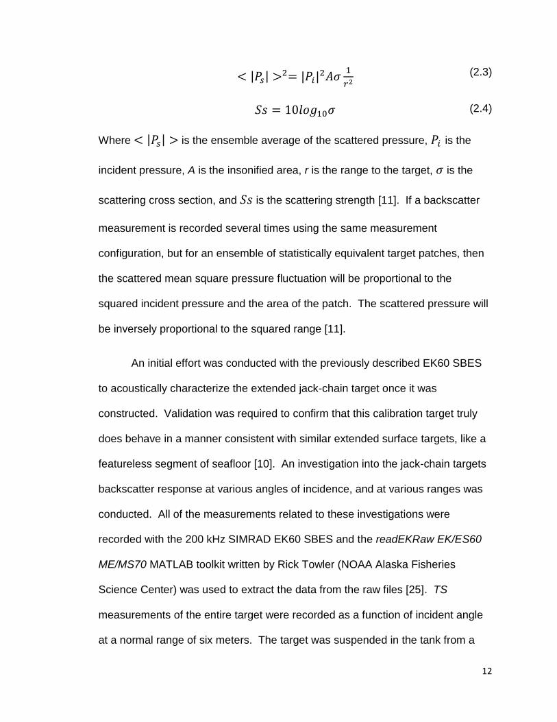
Where is the ensemble average of the scattered pressure, is the

incident pressure, A is the insonified area, r is the range to the target, is the

scattering cross section, and is the scattering strength [11]. If a backscatter

measurement is recorded several times using the same measurement

configuration, but for an ensemble of statistically equivalent target patches, then

the scattered mean square pressure fluctuation will be proportional to the

squared incident pressure and the area of the patch. The scattered pressure will

be inversely proportional to the squared range [11].

An initial effort was conducted with the previously described EK60 SBES

to acoustically characterize the extended jack-chain target once it was

constructed. Validation was required to confirm that this calibration target truly

does behave in a manner consistent with similar extended surface targets, like a

featureless segment of seafloor [10]. An investigation into the jack-chain targets

backscatter response at various angles of incidence, and at various ranges was

conducted. All of the measurements related to these investigations were

recorded with the 200 kHz SIMRAD EK60 SBES and the readEKRaw EK/ES60

ME/MS70 MATLAB toolkit written by Rick Towler (NOAA Alaska Fisheries

Science Center) was used to extract the data from the raw files [25]. TS

measurements of the entire target were recorded as a function of incident angle

at a normal range of six meters. The target was suspended in the tank from a

13

floating platform with the middle of the target at the same depth as the EK60

SBES. This platform was placed at varying positions along the length of the tank

corresponding to 5° incremental changes in the angle of incidence. This concept

is illustrated Figure 2.4.

Figure 2.4 ‒ Positioning of target for angular dependence of Ss investigation (left to right, top to

bottom)

One should look at Figure 2.4 and follow the progression of images

labeled one through four in the bottom right of each panel. Each new target

orientation was a new measurement. A laser level was used to ensure proper

beam alignment to the jack-chain target. The laser level was directed towards a

paper target fixed to the floating platform which corresponded to the chain targets

position underwater. This alignment method is shown in Figure 2.5.

Target Target

Target Target

1 2

3 4

14

Figure 2.5 ‒ Laser level alignment method with paper target corresponding to calibration target position

In Figure 2.5, the laser level is directed towards a paper target fixed to the

floating platform that the extended chain target is suspended from. The laser

aims at a point that corresponds to the middle of the underwater extended chain

target. This alignment method ensures that the beam is incident on the middle of

the target, as shown by Figure 2.6. Figure 2.6 is a drawing to show this

alignment method at six meters.

Laser Level

Paper Target

15

Figure 2.6 ‒ Beam interaction with target

TS values from this experiment show angle dependence with higher TS

values near normal incidence and lower TS values at oblique incidence (Figure

2.7, left), approximately tracking the beam footprint size as it changes with

incidence angle. An average value of all the trials at each angle is included in

Figure 2.7.

16

Ten sets of measurements, or runs, spanning the length of the test tank

were recorded, and are outlined in the legend of Figure 2.7. Average Ss values

show weak or no angle-dependence. This is the expected type of distribution

from a uniformly random target made of many independent scattering elements

where the Central Limit Theorem applies, as described by Urick [26]. The Ss

data was condensed independently of angle and was used to estimate the PDF

of the equivalent amplitude. The PDF is compared to a Rayleigh distribution in

Figure 2.8. The Rayleigh parameter was found to be equal to 0.1025 and was

determined from the maximum likelihood estimates of the empirical Rayleigh

distribution fit to the data.

-50 0 50-55

-50

-45

-40

-35

-30

-25

-20

-15

Angle (degrees)

Ta

rge

t S

tre

ng

th, d

B

Angular Dependance of Target Strength, EK60

-50 0 50-45

-40

-35

-30

-25

-20

-15

-10

Angle (degrees)

Sca

tte

rin

g S

tre

ng

th S

s, d

B

Angular Dependance of Scattering Strength, EK60

run1

run2

run3

run4

run5

run6

run7

run8

run9

run10

dB average

run1

run2

run3

run4

run5

run6

run7

run8

run9

run10

dB average

Figure 2.7 ‒ TS (left) and Ss (right) as a function of incident angle

17

Figure 2.8 ‒ Comparison of the scattered amplitude distribution (blue histogram) with a Rayleigh distribution (red curve)

A Rayleigh distribution is the typical distribution expected of backscatter

over a flat, featureless seabed [11], and qualitative agreement between the data

and a comparison Rayleigh distribution is displayed in Figure 2.8. To further

evaluate this backscatter data, a Kolmogorov-Smirnov statistical test (KS-test)

was employed to confirm the hypothesis of Rayleigh distributed backscatter from

the extended chain target. The KS-test is a non-parametric measure that

describes how well a theoretical CDF (Cumulative Distribution Function) fits the

CDF estimated from observed data [1, 20]. The P value describes how likely it is

that the observed data was drawn from the distribution in question, and can be

0 0.05 0.1 0.15 0.2 0.25 0.3 0.350

1

2

3

4

5

6

7

8

9

absolute value of scattered amplitude

PD

F o

f sca

tte

red

am

plitu

de

Backscatter Distribution

data

Rayleigh distribution

18

determined from the KS-test. If the P value is below 0.05 it would be very

unlikely for the data to be drawn from a Rayleigh distribution. If the P value is

above 0.05, and particularly if it’s well above 0.05, then it is likely that the data

was drawn from a Rayleigh distribution. P was equal to 0.2146 for the SBES

data from the extended chain target, suggesting that the data does fit a Rayleigh

distribution.

The range dependence of the TS and the Ss was investigated. This was

done in order to simulate a narrower beam system, like a 2° x 2° MBES. As the

SBES approaches the chain target, fewer chain links contribute to the

backscatter. This could pose a potential problem with regard to the Central Limit

Theorem. The Central Limit Theorem is significant for the simple seafloor

models presented here, and applies when there are a large number of

independent scattering elements. The Central Limit Theorem may not apply

during measurements that limit the number of contributing scattering elements.

These measurement configurations are similar to what a narrow beam MBES

would experience from a larger range measurement. The jack-chain target was

again suspended from a floating platform and was held stationary at normal

incidence to the EK60 SBES. The powered cart on the bridge of the test tank

was used to vary the range between the SBES and the target. As the range

between the SBES and the target changed, the insonified area would change as

well, thus including different numbers of scattering elements (links). For

example, at two meters approximately 240 links are included in the 7° SBES

19

footprint and at seven meters there are more than 2900 links included. A 2° x 2°

MBES would include roughly 780 links at 8 meters.

Figure 2.9 ‒ TS and Ss as a function of range at normal incidence

Figure 2.9 shows that the TS values increase with range, which is

expected due to the dependence of TS on the insonified area. More scattering

elements are included as the beam footprint grows with range from the target. A

higher signal is returned with more contributing scattering elements, and a higher

TS value is measured. The Ss obtained after compensation of the insonified

area shows a behavior that is independent of the measurement range, confirming

that the measurement configuration is correctly compensated. The trend

displayed in Figure 2.9 shows that the TS depends on the number of active

scattering elements, but the Ss, intrinsic to the target, does not show this

3 4 5 6 7 8

-60

-50

-40

-30

-20

-10

0

Range (m)

Ta

rge

t S

tre

ng

th, d

BNormal Range Dependance of Target Strength, EK60

2 3 4 5 6 7

-50

-40

-30

-20

-10

0

10

Range (m)

Sca

tte

rin

g S

tre

ng

th S

s, d

B

Normal Range Dependance of Scattering Strength, EK60

20

dependence. These SBES range measurements show how the number of

scattering elements included in a measurement has a direct impact on the

measurement value, and that the SBES footprint approximates the footprint of a

narrow beam MBES at close range. Furthermore, these results support the claim

that this target truly does behave in a manner consistent with simple seafloor

models, where the total return pressure is composed of individual contributing

returns from many independent scattering elements.

21

2.3 ‒ Discussion

The results from the jack-chain target showed little dependence between

the angles of incidence and the Ss values, suggesting that the target Ss is

independent of the angle of incidence. This was expected for the extended chain

target because the chain links are suspended in a random orientation. The

backscatter from the target was also found to be Rayleigh distributed from

statistical testing.

The TS values increase with range, which is expected due to the

dependence of TS on the beam footprint. The Ss obtained after compensation of

the insonified area shows a behavior that is independent of the measurement

range, confirming that the measurement configuration is correctly compensated.

This makes the target advantageous in MBES calibration because the Ss value

of the target will be the same for every beam of a MBES. The final Ss value that

is representative of the jack-chain extended target was found to be equal to -16

dB based on the measurements presented in this chapter.

The efforts summarized here are to support the claim that this target is

suitable for MBES calibration. The tests were conducted to show that the Ss

values are independent of measurement geometry and that the TS depends on

the number of active scattering elements. These are all desirable features for

22

calibrating MBES, and the target is justified for use in MBES calibration based on

these claims.

23

CHAPTER 3

MULTI-BEAM ECHO-SOUNDER CALIBRATION

3.1 – Introduction

In MBES operation, hundreds of beams are formed over a wide angular

sector in the athwartship direction by taking the coherent sum of time delayed

return signals originating within the elements of a transmit array and received by

the elements of a co-located receiver array [17]. Seafloor backscatter can be

extracted from each individual beam through the amplitude of the portion of the

complex envelope associated with the seafloor [11].

MBES calibrations can include many parameters like gain and source

level offsets [13]. These are manufacturer applied quantities that can be

calibrated as separate terms. Additional factors must be considered in order to

convert the digital value that is reported from a Reson record into a meaningful

echo-level present at the transducer face [15]. These factors include

transduction, which is the actual conversion of an acoustic pressure wave into an

analog voltage. The process of digitization or converting this analog voltage to a

digital number must be considered as well. Time delay beam-forming is another

factor that requires

24

analysis. These effects are difficult to separate individually, but are able to be

summarized with a “catch-all” calibration coefficient [15]. The calibration

coefficient accounts for many of these topics and is a subject of interest. The

final output of this work is an angle, and thus beam-dependent calibration

coefficient, C, which is calculated from the sonar equation. Approved calibration

results could be applied to backscatter data sets collected with the MBES system

and this would produce calibrated acoustic backscatter.

The MBES system that was calibrated in the UNH tank was a NOAA

owned 200 kHz Reson T20-P MBES (Projector: TC2181, S/N 2413031;

Receiver: S/N 2313068). At 200 kHz the manufacturer states that this system

features a 2° transmit beam-width, and a 2° receive beam-width at broadside. In

the configuration that was used for this effort, 256 beams were spread over a

140° degree swath with a 130µS pulse-length. The MBES transmitter and

receiver are mounted orthogonally to each other. Figure 3.1 shows the mounting

arrangement.

25

Figure 3.1 ‒ T20-P MBES mounting configuration (receiver top, 200 kHz transmitter bottom)

A separate array is used for both the transmitter and the receiver. This

configuration is known as a Mills-Cross [17]. In a Mills-Cross configuration, one

transducer transmits while the other transducer is mounted orthogonally to the

first and acts as the receiver. The resulting beam pattern is the product of the

beam pattern for each transducer. The combined transmit/receive beam pattern

for this arrangement produces a narrow, pencil-like beam as shown in Figure 3.2.

26

Figure 3.2 ‒ Mills-Cross example beam pattern (single beam, receive left, transmit middle, combined right, from Lanzoni [15])

Figure 3.2 shows the region of maximum intensity on-axis for both transmission

and reception. The red areas show the maximum, and side lobes are present in

each picture. This type of directivity has the advantage of producing high angular

resolution in both the alongship and athwartship directions [26].

27

3.2 – Calibration Coefficient Development

As an acoustic pulse is emitted from the transducer, it propagates through

the water column, interacting with the medium along its route until it reaches a

target. Upon the pulse’s arrival at a target, the sound scatters and a portion of

this scattered sound, the backscatter, returns to the transducer. The sonar

equation describes this process in a quantifiable manner, using values presented

in units of decibels (dB), a logarithmic representation of acoustic intensity. The

basic active sonar equation is given by equation 3.1:

(3.1)

where EL is the echo-level at the transducer face in dB (re: 1µPa), SL is the

source level in dB (re: 1µPa), TL is the transmission loss in dB/m (re: 1 ), and

TS is the target strength in dB (re: 1 ), from a reference distance of 1 meter

away from the target [26].

The transmission loss term accounts for the energy lost due to the

spreading and absorption of the acoustic pulse. Equation 3.1 describes the

process for an active acoustic transducer, where the pulse is emitted and

received from the same transducer or transducers that are co-located, thus the

transmission loss is applied twice to account for the two-way travel.

Transmission loss is a function of range and absorption, as shown in equation

3.2:

28

(3.2)

where R is the range from the transducer to the target, and is the absorption

(dB/m).

The target strength is the response of the insonified target and describes

how well the target reflects the incident pulse. This term can be broken into its

constituent components when considering an extended surface target as

previously discussed. In such a case, TS can be defined by equation 3.3.

(3.3)

In this equation, A is the insonified area, and Ss is the surface scattering

strength. The beam footprint near normal incidence is constrained by the beam-

width. The beam-width limited area term for the MBES is displayed in equation

3.4 [19],

(3.4)

where is the transmit beam-width, is the receive beam-width, is the

beam steering angle, and R is the range. The equivalent beam-width was

calculated for both transmission and reception. The equivalent beam-width

accounts for side lobe interaction and models an ideal beam of unity response

within the beam, and zero response outside the beam [17, 23, 26]. Substituting

the sonar equation terms yields the following relation, shown in equation 3.5.

(3.5)

29

The reported EL from a MBES system has some user applied gains which

must be considered. This additional gain term, G, is included in equation 3.6.

(3.6)

A Reson record does not directly measure an echo-level with a user

applied gain. Reson records report some digital value (hereby referred to as DV)

representing the return signal [15]. This DV has units uniquely inherent to the

system and is often left in “Reson units”. The DV includes the measured return,

the user applied gain and any offsets that were previously unaccounted. These

quantities are managed by the “catch all” calibration coefficient, C. This concept

is summarized by equation 3.7 and 3.8.

(3.7)

(3.8)

It is now possible to rearrange this equation and solve for C, which is shown in

equation 3.9:

(3.9)

Once known, the calibration coefficient can be used to convert the DV into

quantities of interest like Ss. The final implementation of this calibration

coefficient is presented in its application to calculate calibrated backscatter. This

is presented in equation 3.10.

(3.10)

30

The Ss values calculated from equation 3.9 incorporate the calibration coefficient

values. These Ss values represent the quantifiable backscatter measurement,

and can be regarded as calibrated backscatter when the calibration coefficients,

C, are applied

31

3.3 ‒ MBES Calibration

Suitable operating parameters for G and SL must be determined to avoid

saturating the system prior to conducting the calibration experiment. Saturation

occurs if the system is operated outside of a linear response regime [7]. The

reported DV is a 16 bit digital number and the dynamic range of a MBES system

is bounded by this limitation. If a return signal is actually more intense than what

the dynamic range of the MBES system can accommodate, then the MBES clips

the signal. This means that the reported DV is less than what the physical return

signal was, and the measurement is ultimately incorrect. Due to this effect, care

must be taken in selecting operating parameters so that saturation may be

avoided. This is done by collecting measurements with various combinations of

G and SL, and then reviewing the data to determine suitable settings. These

measurements were recorded by manually stepping through power and gain

settings in 5 dB increments to determine a suitable linear region within the

working dynamic range of the system. The results of these measurements are

summarized in Figure 3.3.

32

Figure 3.3 ‒ T20-P saturation measurements, gain vs. DV amplitude (dB) for several SL settings

The colors of each curve represent different SL settings, in dB. A hard clip

in the return signal is very obvious at the expected saturation point (96 dB).

Operating parameters were chosen based on these results, and were selected in

a region where the response is linear. Saturation was tested for both the

extended jack-chain target and the reference sphere since measurements would

be recorded from each target. These operational settings are defined in table 1.

Table 1 ‒ T20-P operational settings summary

Target Source Level (SL) Gain Select (G)

Jack-chain extended target

and 38.1mm WC sphere 210 dB 35 dB

0 20 40 60 800

10

20

30

40

50

60

70

80

90

100

X: 35

Y: 65.25

gain (dB)

DV

am

plitu

de

(d

B)

T20-P saturation test w/ 38.1 mm reference sphere

0 20 40 60 8020

30

40

50

60

70

80

90

100

X: 35

Y: 76.69

gain (dB)

DV

am

plitu

de

(d

B)

T20-P saturation test w/ chain target

190

195

200

205

210

215

220

33

The calibration experiment was designed to calibrate every beam of the

system and this was achieved by rotating the array in 1° increments with the

rotator in the test tank facility through 160°, so that all beams were incident on

the chain target. The target was suspended from a floating platform which was

flush to the back wall of the test tank (as illustrated by Figure 3.4), positioning the

target approximately 7.3 meters away from the MBES. The MBES was operated

in “best coverage” or equidistant mode, with a 130 µS long, CW (continuous

wave) pulse. Equidistant mode maintains the distance between beams incident

on a flat target, whereas equiangular mode maintains the angular gap between

beams. The sound speed in the tank was measured next to the MBES active

face with an Odom Digibar Pro sound speed probe, and was then manually input

to the Reson user interface. Absorption in the test tank was equal to 0.01 dB/m,

which was determined from the Francois and Garrison 1982 model [6]. This was

assumed to be negligible at the short ranges permitted for use in the test tank,

and absorption was set to zero in the Reson user interface. The calibration

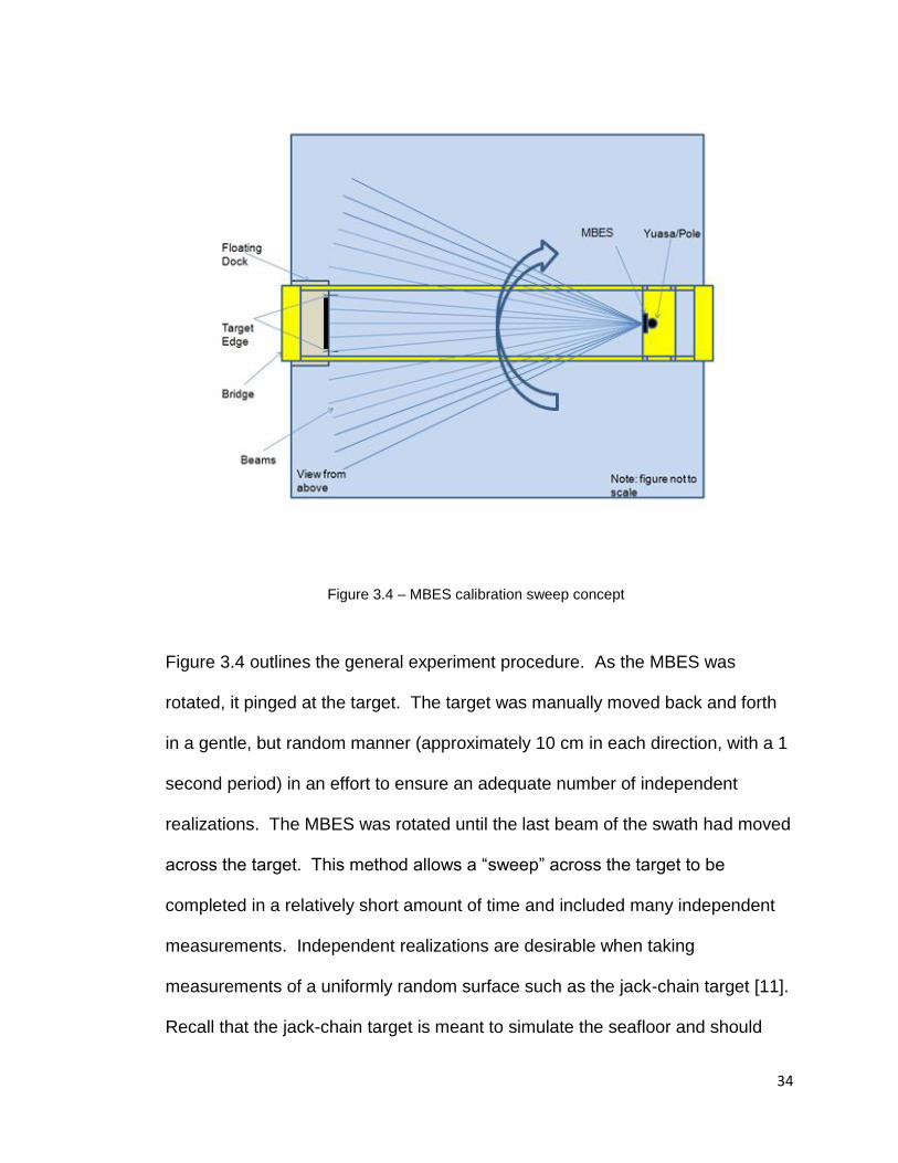
sweep is summarized by Figure 3.4. The sonar was set to ping 30 times per

position, and was triggered by a LabView controller at each new position. The 30

ping setting was selected for statistical robustness, and data were recorded for

every ping.

34

Figure 3.4 ‒ MBES calibration sweep concept

Figure 3.4 outlines the general experiment procedure. As the MBES was

rotated, it pinged at the target. The target was manually moved back and forth

in a gentle, but random manner (approximately 10 cm in each direction, with a 1

second period) in an effort to ensure an adequate number of independent

realizations. The MBES was rotated until the last beam of the swath had moved

across the target. This method allows a “sweep” across the target to be

completed in a relatively short amount of time and included many independent

measurements. Independent realizations are desirable when taking

measurements of a uniformly random surface such as the jack-chain target [11].

Recall that the jack-chain target is meant to simulate the seafloor and should

35

display similar statistics. Independent realizations of the target are required to

truly simulate backscatter from a featureless segment of seafloor.

A library of Reson raw data record readers was used to unpack the data,

and an echogram (single ping) is shown in Figure 3.5.

Figure 3.5 ‒ MBES echogram (single ping, midway through calibration sweep)

The color bar in Figure 3.5 describes the received DV, in dB. The ping

corresponding to the echogram of Figure 3.5 was midway through a calibration

sweep across the target. The target is labeled, and can be found at the

approximate coordinates (5, 6) on the Figure. The back wall of the test tank is

directly behind and parallel to the target. The side wall of the test tank is

MBES

Target

Back Wall

Side Wall

36

orthogonal to the back wall. The distance to the target was known, thus allowing

for precise data acquisition around a specific sample window. The DV data was

then extracted and the calibration coefficient, C was calculated per beam.

A threshold detection was implemented to determine all of the pings at

which a beam was on the target. Once all the pings that returned a DV over the

threshold for a given beam were known, then the median ping from this list was

determined. This median ping was considered to be the ping at which the beam

in question was on the middle of the target. These steps were taken in an effort

to mitigate the risk of including detections that were not fully on target. Once the

middle ping was known, an additional 150 pings were taken on either side of it.

This produces a population of 300 pings per beam spread across the width of the

target, thus ensuring an adequate number of independent realizations. The

boundaries outlining the data that was used are shown in the following figure as

black lines. The purple box is an example to show how the data were averaged

(300 pings for each beam) bounded by the black line. This is displayed in Figure

3.6.

37

Figure 3.6 ‒ Ping progression with data boundaries of 300 pings (black lines)

The color bar in Figure 3.6 describes the received DV, in dB. The 300 ping data

slice that was used for beam 82 is included as an example in Figure 3.7 to

illustrate the independence of each realization.

beam

pin

g

Calibration Sweep, full swath

50 100 150 200 250

500

1000

1500

2000

2500

3000

3500

4000

450020

30

40

50

60

70

80

38

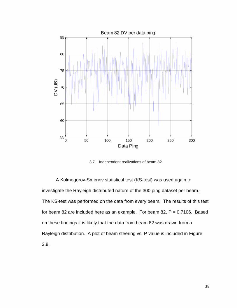
3.7 ‒ Independent realizations of beam 82

A Kolmogorov-Smirnov statistical test (KS-test) was used again to

investigate the Rayleigh distributed nature of the 300 ping dataset per beam.

The KS-test was performed on the data from every beam. The results of this test

for beam 82 are included here as an example. For beam 82, P = 0.7106. Based

on these findings it is likely that the data from beam 82 was drawn from a

Rayleigh distribution. A plot of beam steering vs. P value is included in Figure

3.8.

0 50 100 150 200 250 30055

60

65

70

75

80

85Beam 82 DV per data ping

Data Ping

DV

(d

B)

39

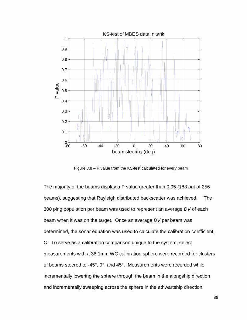
Figure 3.8 ‒ P value from the KS-test calculated for every beam

The majority of the beams display a P value greater than 0.05 (183 out of 256

beams), suggesting that Rayleigh distributed backscatter was achieved. The

300 ping population per beam was used to represent an average DV of each

beam when it was on the target. Once an average DV per beam was

determined, the sonar equation was used to calculate the calibration coefficient,

C. To serve as a calibration comparison unique to the system, select

measurements with a 38.1mm WC calibration sphere were recorded for clusters

of beams steered to -45°, 0°, and 45°. Measurements were recorded while

incrementally lowering the sphere through the beam in the alongship direction

and incrementally sweeping across the sphere in the athwartship direction.

-80 -60 -40 -20 0 20 40 60 800

0.1

0.2

0.3

0.4

0.5

0.6

0.7

0.8

0.9

1

beam steering (deg)

P v

alu

e

KS-test of MBES data in tank

40

These increments provided confidence that measurements were recorded while

the sphere was located on the maximum response axis (MRA) of each beam in a

cluster. Recall that a typical sphere calibration would require a prohibitive

amount of time to complete, so select clusters of beams act as a valid calibration

check and comparison unique to one system that is still relatively time efficient.

The sonar equation was utilized again, but corrected to accommodate a discrete

point target instead of an extended surface target. Thus, the area and Ss terms

are replaced with a known TS value, as shown in equation 3.11.

(3.11)

The ComputeSolidElasticSphere matlab tool [3] was used to model the 38.1 mm

WC calibration sphere that was employed for these measurements. This matlab

tool requires several inputs from the user to accurately calculate the TS of a

calibration sphere. The material of the sphere, sound speed, frequency, and

bandwidth are some of the primary inputs. The TS of the sphere from this model

was found to be equal to -39.2 dB. This value was used in the sonar equation

calculation of C to serve as a comparison to the chain target calibration. Figure

3.9 shows the C value comparisons between both the chain and the spheres.

41

Figure 3.9 ‒ Calibration curve with 38.1 mm WC sphere comparisons at -45°, 0°, and 45°

A meaningful procedure for estimating parameters of random variables

uses the calculation of an interval that includes the estimated parameter and a

known degree of uncertainty [1]. To that end, error was calculated at the 95%

confidence interval and is plotted in red both above and below the calibration

curve results. The upper and lower error bounds were calculated from equations

3.12 and 3.13 respectively,

(3.12)

(3.13)

-80 -60 -40 -20 0 20 40 60 80-120

-118

-116

-114

-112

-110

-108

-106

Beam Steering

C (

dB

)

C Results

C

95% confidence interval upper bound

95% confidence interval lower bound

sphere

42

where is the standard deviation and n is the number of independent pings.

One can see from Figure 3.8 that the sphere C values are close to the 95% error

bound of the calibration sweep C values. Based on these results, the final steps

of this work involve field trials of the T20-P MBES with application of the tank

calibration to the field data.

43

CHAPTER 4

MULTI-BEAM ECHOSOUNDER FIELD TRIALS

4.1 ‒ Field Work with T20-P MBES and EK60 SBES

As a test of the tank calibration methodology, the T20-P MBES was used

to conduct a field survey. This field work effort was part of the greater NEWBEX

(NEWcastle Backscatter EXperiment) project at the Center for Coastal and

Ocean Mapping/Joint Hydrographic Center (CCOM/JHC). The purpose of the

NEWBEX project is to classify and characterize a segment of seafloor local to the

New Hampshire seacoast area. Upon its completion, this characterized segment

of seafloor will serve as a ‘standard line’ that can be run on hydrographic surveys

as a means of confirming proper system performance and monitoring system

health in the field. This standard line is displayed in Figure 4.1 as the thick black

line.

44

Figure 4.1 ‒ NEWBEX standard line route, Portsmouth Harbor, Portsmouth, NH

The R/V Coastal Surveyor (RVCS), a CCOM/JHC owned and operated

coastal research vessel was used to conduct the field work with the T20-P

MBES. The T20-P MBES and the EK60 SBES were mounted to the ram of the

RVCS, with the EK60 positioned at a 45° angle, as shown in Figure 4.2.

Figure 4.2 ‒ Sonar mounting configuration for field deployment

45

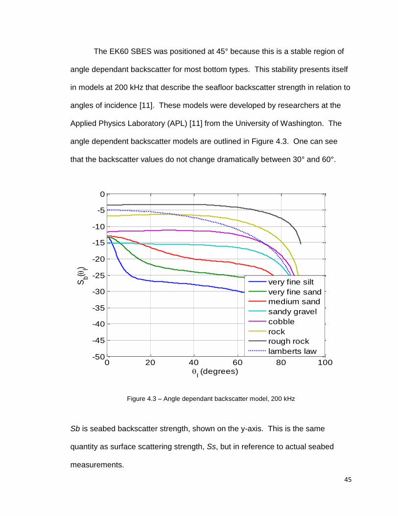
The EK60 SBES was positioned at 45° because this is a stable region of

angle dependant backscatter for most bottom types. This stability presents itself

in models at 200 kHz that describe the seafloor backscatter strength in relation to

angles of incidence [11]. These models were developed by researchers at the

Applied Physics Laboratory (APL) [11] from the University of Washington. The

angle dependent backscatter models are outlined in Figure 4.3. One can see

that the backscatter values do not change dramatically between 30° and 60°.

Figure 4.3 ‒ Angle dependant backscatter model, 200 kHz

Sb is seabed backscatter strength, shown on the y-axis. This is the same

quantity as surface scattering strength, Ss, but in reference to actual seabed

measurements.

0 20 40 60 80 100-50

-45

-40

-35

-30

-25

-20

-15

-10

-5

0

I (degrees)

Sb(

I)

very fine silt

very fine sand

medium sand

sandy gravel

cobble

rock

rough rock

lamberts law

46

A trigger controller was employed between the two systems to alternate

pings between the EK60 SBES and the T20-P MBES. Each system was set to

ping twice per second but the trigger controller alternated between the systems,

producing a total of four soundings on the seafloor per second. The line was run

out to sea and then back to port, recording data continuously. The same

operational settings that were used in the tank for both systems were used again

in the field.

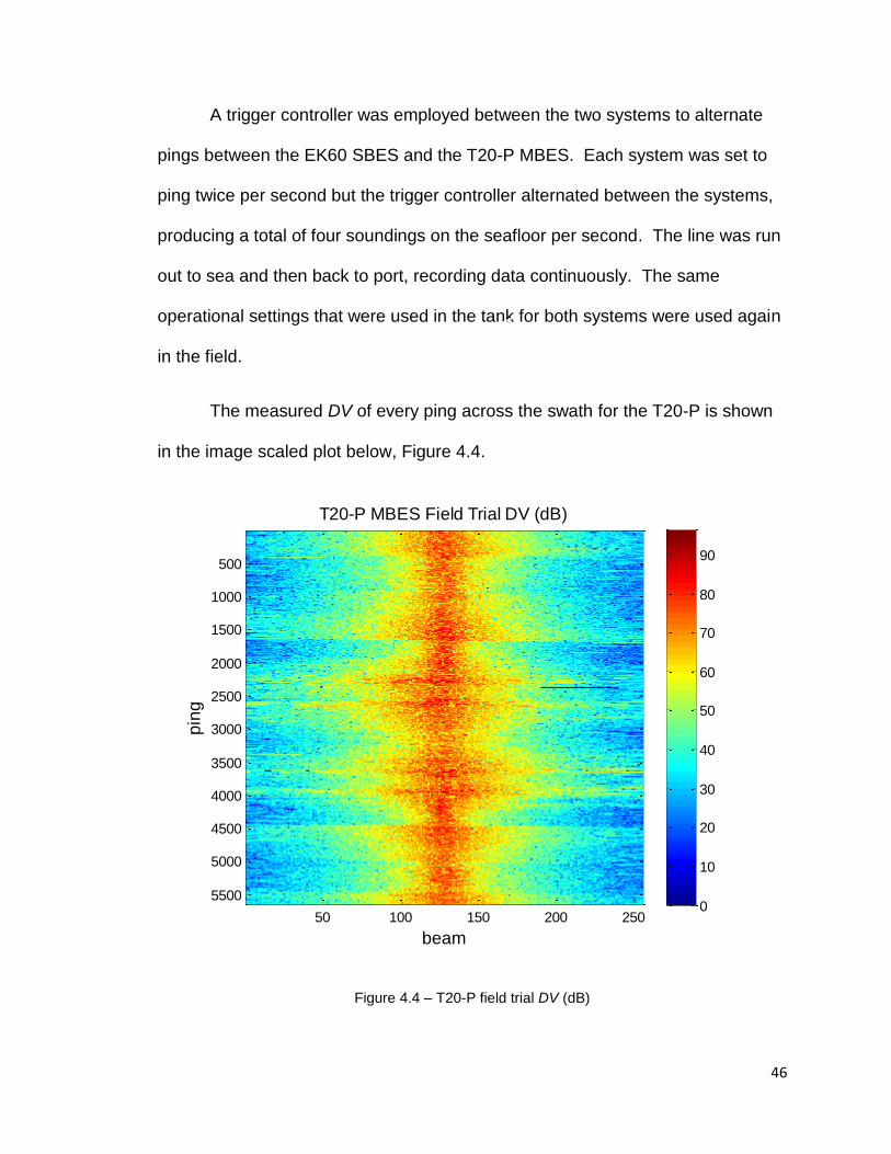
The measured DV of every ping across the swath for the T20-P is shown

in the image scaled plot below, Figure 4.4.

Figure 4.4 ‒ T20-P field trial DV (dB)

beam

pin

g

T20-P MBES Field Trial DV (dB)

50 100 150 200 250

500

1000

1500

2000

2500

3000

3500

4000

4500

5000

55000

10

20

30

40

50

60

70

80

90

47

The quality of these data was then examined by looking for saturation.

Saturation occurs for returns over 96 dB but this data set displayed very few

returns over this value. There were a total of six detections over this limit, and

they were all on the inner, middle beams of the swath (beams 125 to 132), where

returns are expected to be the most intense.

Sb was calculated for both systems using equation 3.10 for each ping,

taking care to apply the correct calibration coefficient from the tank calibration to

the proper beam of the T20-P MBES. Absorption was calculated from the

Francois and Garrison, 1982 model [6] and incorporated into the TL term. Care

was taken on the area calculation in the field. Near normal incidence, the

previously listed beam-width limited area equation was used (equation 3.4). This

was the case for the calibration work in the test tank. However, near oblique

incidence, the beam footprint is typically governed by the pulse length, and

equation 4.2 was used:

(4.1)

where is the sound speed, is the pulse length, is the transmit beam-width,

R is the range, and is the incident angle to the seabed. Equation 4.1 was used

to determine the beam footprint for the Sb comparison in the field, since the MRA

of the EK60 SBES was directed to an incident angle of 45° and this mounting

configuration likely produces a beam that is obliquely incident to the seafloor. A

conservative approach however to ensure that the correct area was used

included calculating the area for both normal and oblique incidence, but using the

48

smaller final value. It is important to note that the data from the T20-P beam that

was steered to 45° (beam 82) was used because that was the beam parallel to

the MRA of the EK60 SBES. This allowed for a meaningful comparison between

systems since the data from both sonar’s came from the same patch of seafloor.

The Sb comparison between the two systems is displayed in Figure 4.5.

Figure 4.5 ‒ Backscatter comparison between EK60 and T20-P beam 82 (steered to -45 , parallel

to EK60 MRA), no averaging

Qualitative agreement is evident between the systems and significant

overlap is clearly displayed. Acoustic backscatter measurements are stochastic

in nature, and each measurement is the result of a sequence of random

processes that are affected by several factors. The dominating factor is the

0 1000 2000 3000 4000 5000 6000-60

-50

-40

-30

-20

-10

0

10

ping

Sb

(d

B)

Sb comparison between systems

EK60

T20-P

49

random nature of the seafloor scattering [11]. Separate clusters of 40 pings (not

a running average) were averaged for each system to produce a more concrete

comparison. The result of this averaging is displayed in Figure 4.6.

Figure 4.6 ‒ Averaged backscatter estimates between EK60 and T20-P, 40 ping clusters

Qualitative agreement is clearly evident between the two systems. Figure 4.7

shows a close up of clusters 25 through 40, and this Figure outlines the

agreement to the 95% confidence interval. The error bound for each system was

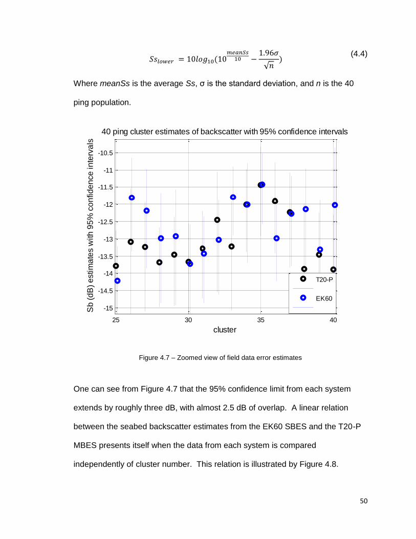
calculated from equations 4.3 and 4.4,

(4.3)

0 50 100 150-28

-26

-24

-22

-20

-18

-16

-14

-12

-10

-8

cluster

Sb

(d

B)

Averaged Backscatter Estimates

EK60

T20-P

50

(4.4)

Where meanSs is the average Ss, σ is the standard deviation, and n is the 40

ping population.

Figure 4.7 ‒ Zoomed view of field data error estimates

One can see from Figure 4.7 that the 95% confidence limit from each system

extends by roughly three dB, with almost 2.5 dB of overlap. A linear relation

between the seabed backscatter estimates from the EK60 SBES and the T20-P

MBES presents itself when the data from each system is compared

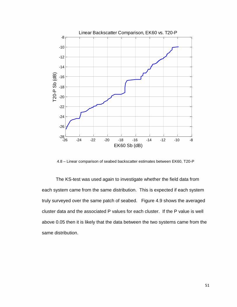
independently of cluster number. This relation is illustrated by Figure 4.8.

25 30 35 40

-15

-14.5

-14

-13.5

-13

-12.5

-12

-11.5

-11

-10.5

cluster

Sb

(d

B)

estim

ate

s w

ith

95

% c

on

fid

en

ce

in

terv

als

40 ping cluster estimates of backscatter with 95% confidence intervals

T20-P

EK60

51

4.8 ‒ Linear comparison of seabed backscatter estimates between EK60, T20-P

The KS-test was used again to investigate whether the field data from

each system came from the same distribution. This is expected if each system

truly surveyed over the same patch of seabed. Figure 4.9 shows the averaged

cluster data and the associated P values for each cluster. If the P value is well

above 0.05 then it is likely that the data between the two systems came from the

same distribution.

-26 -24 -22 -20 -18 -16 -14 -12 -10 -8-28

-26

-24

-22

-20

-18

-16

-14

-12

-10

-8

EK60 Sb (dB)

T2

0-P

Sb

(d

B)

Linear Backscatter Comparison, EK60 vs. T20-P

52

Figure 4.9 ‒ Field data KS-test results

One can see that the P values are all above 0.05, leading one to believe that the

data and results from each sonar system came from the same distribution.

At this point, the results show sufficient agreement between the two

systems, suggesting that the calibration values determined from the tank

experiment for the MBES were executed properly. If that is the case, then the

entirety of the tank calibration curve should be applied to the MBES data to

produce calibrated angle-dependant backscatter for the entire swath instead of

just a single beam. This was done, taking care to use the correct limiting case of

0 50 100 150-30

-20

-10

0

cluster

Sb

(d

B)

Averaged Backscatter Estimates, run 1

EK60

T20-P

0 50 100 1500

0.5

1

P v

alu

e fro

m K

S-t

est

cluster

53

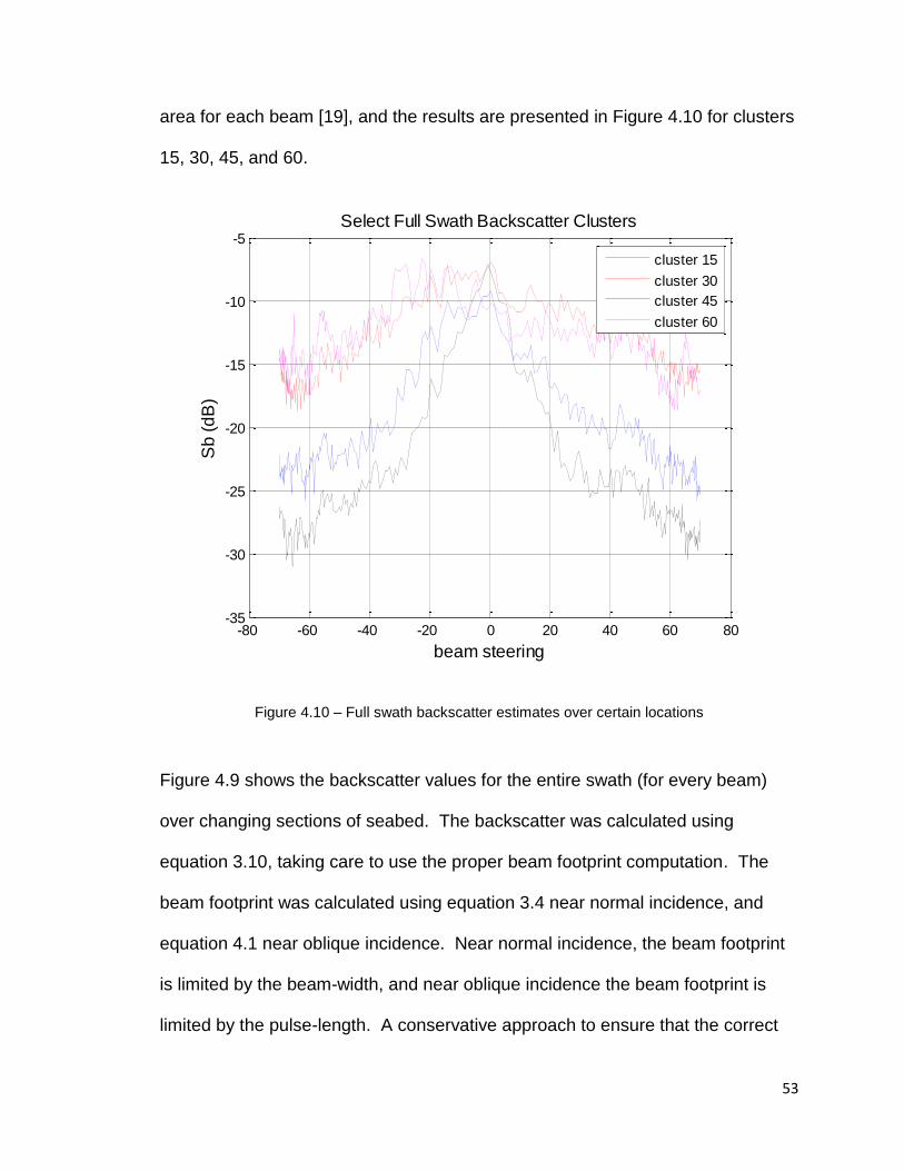
area for each beam [19], and the results are presented in Figure 4.10 for clusters

15, 30, 45, and 60.

Figure 4.10 ‒ Full swath backscatter estimates over certain locations

Figure 4.9 shows the backscatter values for the entire swath (for every beam)

over changing sections of seabed. The backscatter was calculated using

equation 3.10, taking care to use the proper beam footprint computation. The

beam footprint was calculated using equation 3.4 near normal incidence, and

equation 4.1 near oblique incidence. Near normal incidence, the beam footprint

is limited by the beam-width, and near oblique incidence the beam footprint is

limited by the pulse-length. A conservative approach to ensure that the correct

-80 -60 -40 -20 0 20 40 60 80-35

-30

-25

-20

-15

-10

-5

beam steering

Sb

(d

B)

Select Full Swath Backscatter Clusters

cluster 15

cluster 30

cluster 45

cluster 60

54

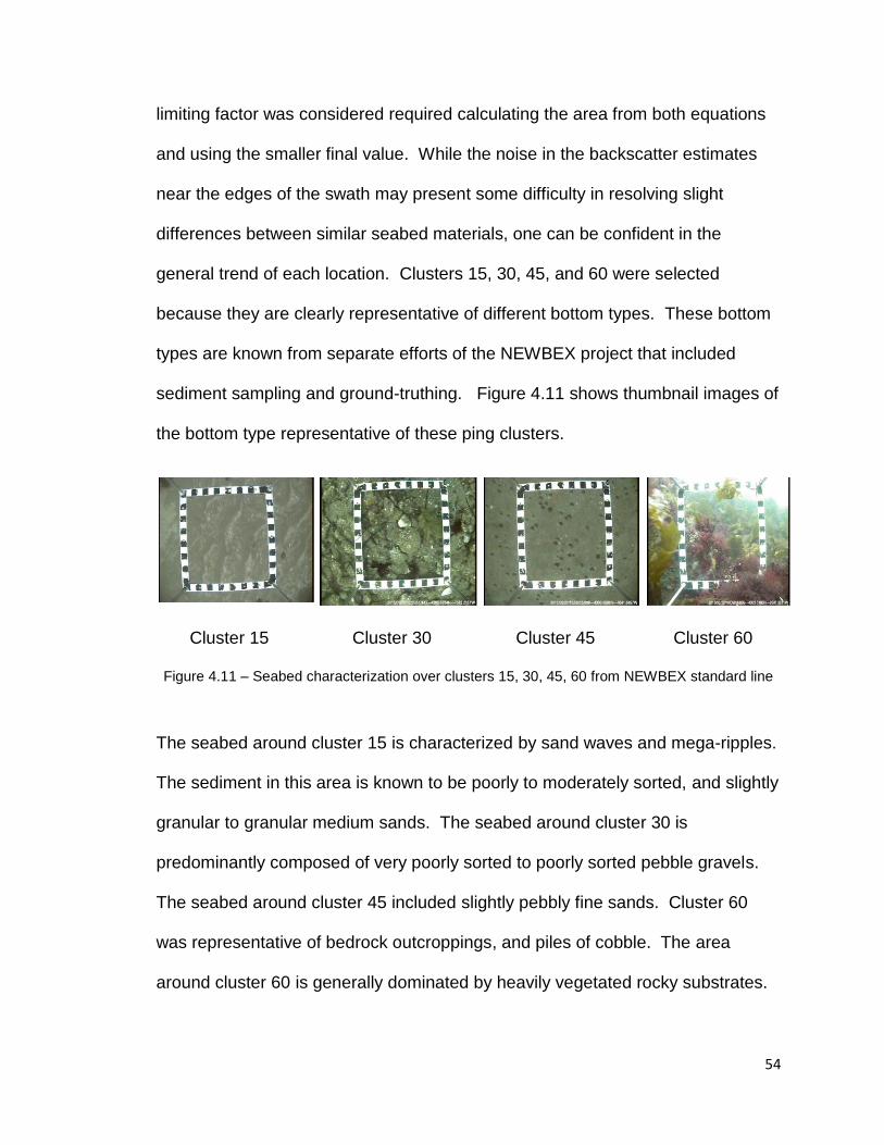
limiting factor was considered required calculating the area from both equations

and using the smaller final value. While the noise in the backscatter estimates

near the edges of the swath may present some difficulty in resolving slight

differences between similar seabed materials, one can be confident in the

general trend of each location. Clusters 15, 30, 45, and 60 were selected

because they are clearly representative of different bottom types. These bottom

types are known from separate efforts of the NEWBEX project that included

sediment sampling and ground-truthing. Figure 4.11 shows thumbnail images of

the bottom type representative of these ping clusters.

Cluster 15 Cluster 30 Cluster 45 Cluster 60

Figure 4.11 ‒ Seabed characterization over clusters 15, 30, 45, 60 from NEWBEX standard line

The seabed around cluster 15 is characterized by sand waves and mega-ripples.

The sediment in this area is known to be poorly to moderately sorted, and slightly

granular to granular medium sands. The seabed around cluster 30 is

predominantly composed of very poorly sorted to poorly sorted pebble gravels.

The seabed around cluster 45 included slightly pebbly fine sands. Cluster 60

was representative of bedrock outcroppings, and piles of cobble. The area

around cluster 60 is generally dominated by heavily vegetated rocky substrates.

55

The locations of these clusters along the line are displayed in Figure 4.12. Point

B corresponds to cluster 15, point C corresponds to cluster 30, point F

corresponds to cluster 45, and point G corresponds to cluster 60.

4.12 ‒ Ping cluster locations along the standard NEWBEX survey line

The ground-truth data supports the angle dependant backscatter that was

calculated and presented in Figure 4.10. Point F (cluster 45) is classified as fine

sand and this location displays the lower backscatter when compared to a harder

target like the bedrock at point G (cluster 60). Additional assurance is provided

when one notes that the APL model included in Figure 4.3 agrees well with the

backscatter calculated in Figure 4.10, and the simple seabed characterizations

56

displayed in Figure 4.11, and Figure 4.12. For example, At 45° cluster 15 reports

backscatter of roughly -22 dB, and the APL model describes this as medium

sand which is in agreement with the NEWBEX provided seafloor characterization

of granular medium sand, described by Figure 4.11.

57

CHAPTER 5

CONCLUSIONS

5.1 ‒ Conclusions and Remarks

The goal of this work was to develop a novel, simple and efficient

methodology for calibrating MBES using an extended calibration target that

replicates the morphology of the seafloor instead of using the typical reference

sphere targets. Multi-beam echo-sounders (MBES) are becoming more frequent

in seafloor mapping applications as well as fisheries and habitat mapping

endeavors. Intensity calibrations are of significant importance with regard to

increasing the utility of MBES backscatter measurements. Intensity calibration

measurements in a tank with standard reference spheres can produce excellent

results, but the amount of time required to complete such measurements is often

prohibitively large. While split-beam echo-sounders (SBES) are able to be

calibrated relatively easily with the tungsten-carbide (WC) reference spheres, it is

significantly more difficult to conduct the same calibration on a MBES because

these systems lack the split-beam capability required to precisely locate a point

target within a beam. An alternative calibration method has been presented

here. The calibration coefficient is a “catch-all” beam dependent value

58

determined from the sonar equation, and is used with regard to intensity

calibrations.

The intensity calibration methodology for MBES proposed here employs

an extended surface target comprised of randomly oriented “jack-chain” links.

This new calibration approach was tested in the fresh water tank of the University

of New Hampshire, demonstrating that it is a potential candidate for alternative

intensity calibration methods. A more easily calibrated 200 kHz SIMRAD EK60

SBES was used to acoustically characterize this extended surface target in order

to investigate any angular and range dependant backscatter. No relation was

found to exist between the angle of incidence and the calculated Ss for the

target. Similarly, the calculated Ss were found to be largely independent of

measurement range to the target.

Once the chain target was acoustically characterized and the backscatter

characteristics were made clear, then the target could be used for an in tank

MBES intensity calibration. The MBES system that was calibrated in the tank

with the chain target was a 200 kHz Reson T20-P. The backscatter from the

chain target was analyzed and found to originate from a Rayleigh distribution.

This is an attractive characteristic for an extended target meant to simulate the

seafloor. Calibration comparison measurements unique to the T20-P MBES

were recorded for select clusters of beams with a standard 38.1 mm tungsten

carbide reference sphere. The sphere was measured on axis and provided a

way to check the calibration curve generated from the chain target at particular

points in the swath.

59

Agreement between the calibration values determined from the chain

target and the WC sphere was satisfactory, and both systems were brought to

sea for a field experiment. The calibration produced in the tank was meant to be

applied to a set of field data to produce calibrated seabed backscatter estimates

over a previously characterized patch of seabed, or ‘standard line’. Seabed

backscatter estimates (Sb) should match between both systems once the tank

calibration is applied to the MBES. Both the EK60 SBES and T20-P MBES were

mounted to the ram of the UNH CCOM/JHC owned and operated R/V Coastal

Surveyor. The systems made use of a trigger controller to regulate the ping rates

of each system and a survey was run over a standard line in Portsmouth Harbor,

Portsmouth, NH. Seabed backscatter results agree at the 95% confidence

interval and the data from each system was shown to come from the same

underlying distributions, thus confirming that the goal of this work has been

achieved. Calibrated intensity measurements have successfully been attained,

and were achieved in a condensed amount of time than previous intensity

calibration methods could be completed. One calibration sweep was all that was

required for this work. While the results of this work are promising, there are

some limitations to this proposed calibration methodology that must be

addressed. As it stands, this calibration method requires a custom built extended

target, and a test tank facility. Meeting these requirements may be unrealistic for

some users.

Further research should include considerations into an automated

dynamic agitator for the chain target during any tank calibration work. The chain

60

target was manually moved back and forth, approximately 10 cm/s to provide an

adequate number of independent realizations of the target. This type of manual

movement, while sufficient for the purposes of this experiment lacks a precise

quantifiable measurement of movement. Additional further research could be

done to apply this extended target calibration method to field calibrations.

Present field calibrations use the same reference sphere targets that were

described in this thesis [14]. The same difficulties that were present in a

controlled test tank environment exist for field calibrations as well. A sphere

must be suspended from flexible rods fixed to a vessel and moved along beams

directed toward the seabed in both the alongship and athwartship directions.

This is done all while the sonar is mounted to the hull, or ram of the vessel. It

may be possible to implement a field calibration version of this extended target to

ease the complications of calibrating on a vessel. A smaller version of the jack-

chain extended target could be suspended from these flexible rods, and

positioned under the vessel in a manner where it would be parallel to a flat

seafloor. If the MBES were fixed to a mount that could precisely rotate the

system around the roll axis of the vessel, then a similar calibration sweep could

be completed.

61

REFERENCES

62

LIST OF REFERENCES

[1] J.S.Bendat, A.G. Piersol, “Random Data: Analysis and Measurement Procedures”, Third Edition, Wiley Publishing, 2000 [2] C. Brown, P. Blondel, “Developments in the application of multibeam sonar backscatter for seafloor habitat mapping”, Applied Acoustics 70 (2009) 1242-1247 [3] D. Chu, “TS Package”, ComputeSolidElasticSphereTS Matlab GUI, NOAA [4] Foote, K.G., et al. “Calibration of Acoustic Instruments for Fish Density Estimation: A Practical Guide”, No. 144. International Council for the Exploration of the Sea, 1987 [5] Foote, K. G., et al. “Protocols for Calibrating Multibeam Sonar”, the Journal of the Acoustical Society of America, 117, 2005 [6] Francois, Garrison, Calculation of absorption of sound in seawater, 1982 model, [online], Available: http://resource.npl.co.uk/acoustics/techguides/seaabsorption/ [7]S.F. Greenaway, “Linearity Tests of A Multibeam Echosounder”, MS Thesis, Center for Ocean and Coastal Mapping/Joint Hydrographic Center, University of New Hampshire, 2010 [8] S.F. Greenaway and T.C. Weber, “Test Methodology for Evaluation of Linearity of Multibeam Echosounder Backscatter Performance”, Proc. MTS/IEEE Oceans 2010 Conf., Sep. 20-23, Seattle, WA [9] E. Hammerstad, EM Technical Note, “Backscattering and Seabed Image Reflectivity”, 2000

63

[10] J. Heaton, T. Weber, G. Rice, X. Lurton, “Testing of an extended target for use in high frequency sonar calibration”, Conference Proceedings, J. Acoust. Soc. Am., Vol. 133, No. 5, Pt. 2, May 2013 [11] D. R. Jackson, M. D. Richardson, “High Frequency Seafloor Acoustics”, Springer Publishing, 2007 [12] L.E. Kinsler, A.R. Frey, A.B. Coppens, and J.V. Sanders, “Fundamentals of Acoustics,” 4th ed., Wiley, New York, 2000 [13] J.C. Lanzoni and T.C. Weber, “Calibration of multibeam echo sounders: a comparison between two methodologies”, Proc. of Meetings on Acoustics, vol.17, pp.070040, Dec. 2012. [14] J.C. Lanzoni, T.C. Weber, “High-resolution Calibration of a Multibeam Echo Sounder”, Proc. MTS/IEEE Oceans 2010 Conf., Sep. 20-23, Seattle, WA [15] J. C. Lanzoni, T. C. Weber, “A Method for Field Calibration of a Multibeam Echo Sounder”, MS Thesis, Center for Ocean and Coastal Mapping/Joint Hydrographic Center, University of New Hampshire, 2011 [16] J.C. Lanzoni, T.C. Weber, “Reson Seabat 7125 Multibeam Sonar System Calibration”, Center for Coastal and Ocean Mapping/Joint Hydrographic Center, University of New Hampshire, 2013 [17] X. Lurton, “An Introduction to Underwater Acoustics”, Praxis Publishing, 2010 [18] X. Lurton, “Swath Bathymetry Using Phase Difference: Theoretical Analysis of Acoustical Measurement Precision”, IEEE Journal of Ocean Engineering, Vol. 25, No. 3, 2000 [19] X. Lurton, S. Dugelay, J.M. Augustin, “Analysis of multibeam echo-sounder signals from the deep seafloor”, IEEE, 0-7803-2056-5, 1994

64

[20] A.P. Lyons, D.A. Abraham, “Statistical characterization of high-frequency shallow-water seafloor backscatter”, J. Acoust. Soc. Am. 106, September 1999 [21] I. Parnum, A. Gavrilov, “High-frequency multibeam echo-sounder measurements of seafloor backscatter in shallow water: Part 1 – Data acquisition and processing”, International Journal of the Society for Underwater Technology, Vol. 30, No. 1, pp 3-12, 2011

[22] Rossing, Moore, Wheeler, “The Science of Sound”, 3rd edition, Addison Wesley Publishing, 2002 [23] J. Simmonds, D. MacLennan, “Fisheries Acoustics: Theory and Practice”, second edition, Blackwell Publishing, 2005 [24] W.T. Thomson, M.D. Dahleh, “Theory of Vibration with Applications”, 5th Edition, Prentice Hall Publishing, 1998 [25] R. Towler, readEKRaw EK/ES60 ME/MS 70 Matlab toolkit, NOAA Alaska Fisheries Science Center, [Online], Available: http://www.hydroacoustics.net/viewtopic.php?f=36&t=131&start=0

[26] R.J. Urick, “Principles of Underwater Sound,” 3rd ed., McGraw–Hill, New York, 1998 [27] B. Welton, “Backscatter Measurement Variation between NOAA’s Reson 7125 Multibeams and a Method for a Relative Field Ca libration between Systems”, MS Thesis, University of New Hampshire, 2014

65