Utility Indifference Pricing - An Overview

Vicky Henderson 0

Princeton University

David Hobson 1

University of Bath

August 2004

to appear in Volume on Indifference Pricing, (ed. R. Carmona), Princeton University Press

0ORFE and Bendheim Center for Finance, E-Quad, Princeton University, Princeton, NJ. 08544. USA.vhenders@princeton.edu

1Department of Mathematical Sciences, University of Bath, Bath. BA2 7AY. UK. dgh@maths.bath.ac.uk

1 Introduction

The idea of gamblers ranking risky lotteries by their expected utilities dates back to Bernoulli[4]. An individual’s certainty equivalent amount is the certain amount of money that makesthem indifferent between the return from the gamble and this amount, as described in Chapter6 of Mas-Colell et al [59]. Certainty equivalent amounts and the principle of equi-marginalutility (see Jevons [49]) have been used by economists for many years.

More recently, these concepts have been adapted for derivative security pricing. Consideran investor receiving a particular derivative or contingent claim offering payoff CT at futuretime T > 0. When there is a financial market, and the market is complete, the price theinvestor would pay can be found uniquely. Option pricing in complete markets uses the ideaof replication whereby a portfolio in stocks and bonds re-creates the terminal payoff of theoption thus removing all risk and uncertainty. The unique price of the option is given bythe law of one price - the initial wealth necessary to fund the replicating portfolio. However,in reality, most situations are incomplete and complete models are only an approximationto this. Market frictions, for example transactions costs, non-traded assets and portfolioconstraints, make perfect replication impossible. In such situations, many different optionprices are consistent with no-arbitrage, each corresponding to a different martingale measure.There is no longer a unique price.

However, in this situation, even with an incomplete financial market, the investor canmaximize expected utility of wealth and may be able to reduce the risk due to the uncertainpayoff through dynamic trading. She would be willing to pay a certain amount today forthe right to receive the claim such that she is no worse off in expected utility terms thanshe would have been without the claim. Hodges and Neuberger [44] were the first to adaptthe static certainty equivalence concept to a dynamic setting like the one described. Similarideas are also important in actuarial mathematics. There is a valuation method called the“premium principle of equivalent utility” which has desirable properties if utility is of theexponential form, see Gerber [30] for details. The method described above, termed utilityindifference pricing, and the subject of this book, is one approach that can be taken in anincomplete market.

Other potential approaches which will be discussed in this overview include superrepli-cation, the selection of one particular measure according to a minimal distance criteria (forexample the minimal martingale measure or the minimal entropy measure) and convex riskmeasures.

The advantages of utility indifference pricing include its economic justification and in-corporation of risk aversion. It leads to a price which is non-linear in the number of unitsof claim, which is in contrast to prices in complete markets and some of the alternativesmentioned above. The indifference price reduces to the complete market price which is anecessary feature of any good pricing mechanism. Indifference prices can also incorporatewealth dependence. This may be desirable as the price an investor is willing to pay couldwell depend on the current position of his derivative book. Although we concentrate on pric-ing issues here, utility indifference also gives an explicit identification of the hedge position.This is found naturally as part of the optimization problem.

Limitations of indifference pricing methodology include the fact that explicit calculationsmay be done in only a few concrete models, mainly for exponential utility. Exponential utilityhas the feature that the wealth or initial endowment of the investor factors out of the problem

1

which makes the mathematics tractable but is also a strong assumption. Different investorswith varying initial wealths are unlikely to assign the same value to a claim. Practically, usersmay not be satisfied with the concept of utility functions and unable to specify the requiredrisk aversion coefficient.

In this overview, we will introduce utility indifference pricing and give a survey of theliterature, both more theoretical and applications. Inevitably, such a survey reflects theauthors’ experience and interests.

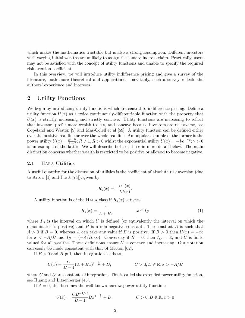
2 Utility Functions

We begin by introducing utility functions which are central to indifference pricing. Define autility function U(x) as a twice continuously-differentiable function with the property thatU(x) is strictly increasing and strictly concave. Utility functions are increasing to reflectthat investors prefer more wealth to less, and concave because investors are risk-averse, seeCopeland and Weston [9] and Mas-Colell et al [59]. A utility function can be defined eitherover the positive real line or over the whole real line. An popular example of the former is thepower utility U(x) = x1−R

1−R ;R 6= 1, R > 0 whilst the exponential utility U(x) = − 1γ e

−γx; γ > 0is an example of the latter. We will describe both of these in more detail below. The maindistinction concerns whether wealth is restricted to be positive or allowed to become negative.

2.1 Hara Utilities

A useful quantity for the discussion of utilities is the coefficient of absolute risk aversion (dueto Arrow [1] and Pratt [74]), given by

Ra(x) = −U′′(x)

U ′(x).

A utility function is of the Hara class if Ra(x) satisfies

Ra(x) =1

A+Bxx ∈ ID (1)

where ID is the interval on which U is defined (or equivalently the interval on which thedenominator is positive) and B is a non-negative constant. The constant A is such thatA > 0 if B = 0, whereas A can take any value if B is positive. If B > 0 then U(x) = −∞for x < −A/B and ID = (−A/B,∞). Conversely if B = 0, then ID = R, and U is finitevalued for all wealths. These definitions ensure U is concave and increasing. Our notationcan easily be made consistent with that of Merton [62].

If B > 0 and B 6= 1, then integration leads to

U(x) =C

B − 1(A+Bx)1−

1B +D; C > 0, D ∈ R, x > −A/B

where C andD are constants of integration. This is called the extended power utility function,see Huang and Litzenberger [45].

If A = 0, this becomes the well known narrow power utility function:

U(x) =CB−1/B

B − 1Bx1− 1

B +D; C > 0, D ∈ R, x > 0

2

It is more usually written with R = 1/B and D = 0, C = B1/B, giving

U(x) =x1−R

1−RR 6= 1.

The narrow power utility has constant relative risk aversion of R, where relative risk aversionRr(x) is defined to be Rr(x) = xRa(x).

Returning to further utility functions in the Hara class, for B = 1 we have

U(x) = C ln (A+ x) + E C > 0, E ∈ R, x > −A,

the logarithmic utility function. Taking A = 0, E = 0, C = 1 gives the standard or narrowform.

Finally, for B = 0

U(x) = −FAe−x/A +G F > 0, A > 0, G ∈ R, x ∈ R,

the exponential utility function. It is usual to take G = 0, A = 1/γ, F = 1/γ2. For this utilityfunction, Ra(x) = γ, a constant.

2.2 Non-Hara Utilities

We now briefly discuss some utility functions which do not fit into the Hara class. Animportant example is the quadratic utility which has received much attention historically inthe literature. Taking B = −1, A > 0 in (1) gives

U(x) = x− 12A

x2 x ∈ R

This decreases over part of the range, violating the assumption that investors desire morewealth and so have an increasing utility function, but has excellent tractability properties.

When used to price options, some of the common utility functions discussed in the previoussections have shortcomings. For instance, we shall show that it is not possible to price a shortcall option with exponential or power type utilities. The power utility requires wealth be non-negative and the exponential, although allowing for negative wealth, gives problems at least inthe case of lognormal models. To circumvent these problems, it is worth mentioning anothermoderately tractable family of utilities. These are functions of the form:

U(x) =1κ

(1 + κx−

√1 + κ2x2

); κ > 0 (2)

This class penalises negative wealth less severely.We will also briefly introduce some special utilities related to other methodologies for

pricing in incomplete markets. Firstly, consider the concept of super-replication. A claimis super-replicated if the hedging portfolio is guaranteed to produce at least the payoff ofthe claim. The super-replication price is the smallest initial fortune with which it is possibleto super-replicate the payoff of the claim with probability one. It is the supremum of thepossible prices consistent with no arbitrage, and is therefore often unrealistically high. Thesuper-replication price corresponds to a utility function of the form

U(x) =−∞ x < 00 x ≥ 0

3

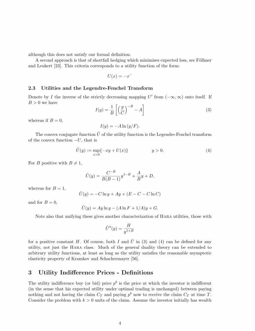
although this does not satisfy our formal definition.A second approach is that of shortfall hedging which minimises expected loss, see Follmer

and Leukert [23]. This criteria corresponds to a utility function of the form:

U(x) = −x−

2.3 Utilities and the Legendre-Fenchel Transform

Denote by I the inverse of the strictly decreasing mapping U ′ from (−∞,∞) onto itself. IfB > 0 we have

I(y) =1B

[( yC

)−B−A

](3)

whereas if B = 0,I(y) = −A ln (y/F ).

The convex conjugate function U of the utility function is the Legendre-Fenchel transformof the convex function −U , that is

U(y) := supx>0

−xy + U(x) y > 0. (4)

For B positive with B 6= 1,

U(y) =C−B

B(B − 1)y1−B +

A

By +D,

whereas for B = 1,U(y) = −C ln y +Ay + (E − C − C lnC)

and for B = 0,U(y) = Ay ln y − (A lnF + 1/A)y +G.

Note also that unifying these gives another characterization of Hara utilities, those with

U ′′(y) =H

y1+B

for a positive constant H. Of course, both I and U in (3) and (4) can be defined for anyutility, not just the Hara class. Much of the general duality theory can be extended toarbitrary utility functions, at least as long as the utility satisfies the reasonable asymptoticelasticity property of Kramkov and Schachermayer [56].

3 Utility Indifference Prices - Definitions

The utility indifference buy (or bid) price pb is the price at which the investor is indifferent(in the sense that his expected utility under optimal trading is unchanged) between payingnothing and not having the claim CT and paying pb now to receive the claim CT at time T .Consider the problem with k > 0 units of the claim. Assume the investor initially has wealth

4

x and zero endowment of the claim. The definitions extend to cover non-zero endowmentsalso. Define

V (x, k) = supXT∈A(x)

EU(XT + kCT ) (5)

where the supremum is taken over all wealths XT which can be generated from initial fortunex. The utility indifference buy price pb(k) is the solution to

V (x− pb(k), k) = V (x, 0). (6)

That is, the investor is willing to pay at most the amount pb(k) today for k units of theclaim CT at time T . Similarly, the utility indifference sell (or ask) price ps(k) is the smallestamount the investor is willing to accept in order to sell k units of CT . That is, ps(k) solves

V (x+ ps(k),−k) = V (x, 0). (7)

Formally, the definitions of these two quantities can be related by pb(k) = −ps(−k), and withthis in mind, we let p(k) denote the solution to (6) for all k ∈ R.

Utility indifference prices are also known as reservation prices, for example, see Munk [66].Also used in the finance literature is the terminology “private valuation”, which emphasizesthe proposed price is for an individual with particular risk preferences, see Tepla [82] andDetemple and Sundaresan [18].

Utility indifference prices have a number of appealing properties. We will comment furtheron these properties later in specific model frameworks.(i) Non-linear pricingFirstly, in contrast to the Black and Scholes price (and many alternative pricing methodologiesin incomplete markets), utility indifference prices are non-linear in the number of options, k.The investor is not willing to pay twice as much for twice as many options, but requires areduction in this price to take on the additional risk. Alternatively, a seller requires morethan twice the price for taking on twice the risk. This property can be seen from the valuefunction (5) since U is a concave function. Put differently, the amount an agent is preparedto pay for a claim CT depends on his prior exposure to non-replicable risk. We will assumethroughout that this prior exposure is zero, and some of our conclusions (such as concavitybelow) depend crucially on this assumption.(ii) Recovery of complete market priceIf the market is complete or if the claim CT is replicable, the utility indifference price p(k)is equivalent to the complete market price for k units. To show this, let RT denote thetime T value of one unit of currency invested at time 0. If XT ∈ A(x), then we can writeXT = xRT +XT for some XT ∈ A(0), where A(0) is the set of claims which can be replicatedwith zero initial wealth. (We assume that XT ∈ A(0) if and only if XT +xRT ∈ A(x).) SinceCT is replicable, from an initial fortune pBS , write CT = pBSRT + XC

T where XCT ∈ A(0).

The superscript BS is intended to denote the Black Scholes or complete market price. Thenfor XT ∈ A(x),

XT + kCT = (x+ kpBS)RT + XT + kXCT = (x+ kpBS)RT + X ′

T

where X ′T ∈ A(0). Thus XT + kCT ∈ A(x+ kpBS) and so

V (x, k) = supXT∈A(x)

EU(XT + kCT ) = supXT∈A(x+kpBS)

EU(XT ) = V (x+ kpBS , 0)

5

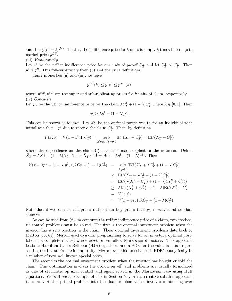
and thus p(k) = kpBS . That is, the indifference price for k units is simply k times the competemarket price pBS .(iii) MonotonicityLet pi be the utility indifference price for one unit of payoff Ci

T and let C1T ≤ C2

T . Thenp1 ≤ p2. This follows directly from (5) and the price definitions.

Using properties (ii) and (iii), we have

psub(k) ≤ p(k) ≤ psup(k)

where psup, psub are the super and sub-replicating prices for k units of claim, respectively.(iv) ConcavityLet pλ be the utility indifference price for the claim λC1

T + (1− λ)C2T where λ ∈ [0, 1]. Then

pλ ≥ λp1 + (1− λ)p2.

This can be shown as follows. Let XiT be the optimal target wealth for an individual with

initial wealth x− pi due to receive the claim CiT . Then, by definition

V (x, 0) = V (x− pi, 1, CiT ) = sup

XT∈A(x−pi)

EU(XT + CiT ) = EU(Xi

T + CiT )

where the dependence on the claim CiT has been made explicit in the notation. Define

XT = λX1T + (1− λ)X2

T . Then XT ∈ A = A(x− λp1 − (1− λ)p2). Then

V (x− λp1 − (1− λ)p2, 1, λC1T + (1− λ)C2

T ) = supXT∈A

EU(XT + λC1T + (1− λ)C2

T )

≥ EU(XT + λC1T + (1− λ)C2

T )= EU(λ(X1

T + C1T ) + (1− λ)(X2

T + C2T ))

≥ λEU(X1T + C2

T ) + (1− λ)EU(X2T + C2

T )= V (x, 0)= V (x− pλ, 1, λC1

T + (1− λ)C2T )

Note that if we consider sell prices rather than buy prices then pλ is convex rather thanconcave.

As can be seen from (6), to compute the utility indifference price of a claim, two stochas-tic control problems must be solved. The first is the optimal investment problem when theinvestor has a zero position in the claim. These optimal investment problems date back toMerton [60, 61]. Merton used dynamic programming to solve for an investor’s optimal port-folio in a complete market where asset prices follow Markovian diffusions. This approachleads to Hamilton Jacobi Bellman (HJB) equations and a PDE for the value function repre-senting the investor’s maximum utility. Merton was able to solve such PDE’s analytically ina number of now well known special cases.

The second is the optimal investment problem when the investor has bought or sold theclaim. This optimization involves the option payoff, and problems are usually formulatedas one of stochastic optimal control and again solved in the Markovian case using HJBequations. We will see an example of this in Section 5.4. An alternative solution approachis to convert this primal problem into the dual problem which involves minimizing over

6

martingale measures, see Section 5.5. Under this approach, the problems are no longerrestricted to be Markovian in nature.

As well as the utility indifference price of the option, the hedging strategy of the investoris crucial. Since the market is incomplete, the hedge will not be perfect. The investor’s hedgearises from the optimization problem (5) where the optimization takes place over admissiblestrategies. The hedge typically involves a Merton term which would be the appropriate hedgefor the no-option problem and an additional term which accounts for the option position.

The remaining concept to introduce is that of the marginal price. The marginal price isthe utility indifference price for an infinitesimal quantity. As we will see later, marginal pricesare linear pricing rules and amount to choosing a particular martingale measure. Marginalprices are commonly used in economics, and have been proposed in an option pricing contextin various forms by Davis [11, 12], Karatzas and Kou [53] and Kallsen [52].

4 Discrete Time Approach to Utility Indifference Pricing

The problem of pricing European options on non-traded assets in a binomial model wasfirst tackled in Smith and Nau [79] in the context of real options and by Detemple andSundaresan [18] as part of a study of the effect of portfolio constraints, see Section 6.2. Bothpapers consider options on a non-traded asset where a second, correlated asset is availablefor trading. Smith and Nau [79] treat European options where the investor has exponentialutility. Detemple and Sundaresan [18] represent price movements in a trinomial model whichthey solve numerically for the utility indifference price in the case of power utility. They alsoconsider American style options but in a simpler framework with no traded correlated asset.In this case, the investor cannot short-sell the underlying asset and indifference prices arefound numerically.

More recently, Musiela and Zariphopoulou [71] (and Chapter 1 of this book) revisit theproblem and place it in a mathematical setting. They derive the European option’s indiffer-ence value in the European case with exponential utility. Other utilities and the alternativedual approach are used in Chapter 2.

We can illustrate briefly the main ideas in a simple one-period binomial model wherecurrent time is denoted 0 and the terminal date is time 1. This exposition follows that ofMusiela and Zariphopoulou [71]. The market consists of a riskless asset, a traded asset withprice P0 today and a non-traded asset with price Y0 today. Assume the riskless asset paysno interest for simplicity. The traded price P0 may move up to P0ψ

u or down to P0ψd where

the random variable ψ takes either value ψu, ψd and 0 < ψd < 1 < ψu. The non-tradedprice satisfies Y1 = Y0φ where φ = φd, φu and φd < φu. There are four states of naturecorresponding to outcomes of the pair of random variables: (ψu, φu), (ψu, φd), (ψd, φu),(ψd, φd). Wealth X1 at time 1 is given by X1 = β + αP1 = x + α(P1 − P0) where α is thenumber of shares of stock held, β is the money in the riskless asset and x is initial wealth.The investor is pricing k units of a claim with payoff C1 and has exponential utility. Thevalue function in (5) becomes

V (x, k) = supα

E[−1γe−γ(X1+kC1)

]

7

and the utility indifference buy price defined in (6) solves

V (x, 0) = V (x− pb(k), k).

The price pb(k) is given by

pb(k) = EQ〈0〉(

1γ

log EQ〈0〉(eγkCT |P1)

)(8)

where Q〈0〉 is the measure under which the traded asset P is a martingale and the conditionaldistribution of the non-traded asset given the traded one is preserved with respect to the realworld measure P. This is the minimal martingale measure of Follmer and Schweizer [25]. Infact, in this simple setting, all minimal distance measures are identical, so Q〈0〉 is also theminimal entropy measure of Frittelli [28], see the discussion in Section 7.2.

The price in (8) can be shown to satisfy properties (i)-(iv) in Section 3, see Chapter 1 ofthis book. The above formulation shows the utility indifference price (in a one period modelwith exponential utility) can be written as a new non-linear, risk adjusted payoff, and thenexpectations are taken with respect to Q〈0〉 of this new payoff. This is in contrast to the usuallinear pricing structures found in complete markets and in other approaches to incompletemarkets pricing. A similar representation appears in Smith and Nau [79].

5 Utility Indifference Pricing in Continuous time.

Consider a model on a stochastic basis (Ω, (Ft)0≤t≤T ,P). For simplicity we assume that themodel supports a single traded asset with price process Pt and a second auxiliary process Yt,which may correspond to a related but non-traded stock or a diffusion process which drivesthe dynamics of Pt. For example Yt may represent the volatility of P . Suppose that Pt andYt are governed by the SDEs

dPt

Pt= σt(dBt + λtdt) + rtdt (9)

dYt = atdWt + btdt (10)

Here B andW are Brownian motions with correlation ρt which together generate the filtrationFt and σ, λ, r, a, b and ρ are adapted to Ft. The problem is to price a (typically non-negative)contingent claim CT ∈ mFT , where T is the horizon time.

We will concentrate on this bi-variate model which is rich enough to contain interestingexamples and to illustrate the central concepts of the theory, but simple enough for explicitsolutions to sometimes exist. It is possible to extend the analysis to higher dimensions, but aswe shall see it is already difficult to find solutions to the utility indifference pricing problemeven in the two-dimensional special case. Throughout this overview we will assume that eventhough the asset Yt is not directly traded, its value is an observable quantity. When Yt is ahidden Markov process and its value needs to be estimated from the information containedin the filtration generated by the traded asset Pt the issues become much more delicate, seeChapter 4.

It is convenient to write the Brownian motion W as a composition of two independentBrownian motions Bt and B⊥

t so that dWt = ρtdBt+ρ⊥t dB⊥t where ρ⊥t is the positive solution

8

to ρ2t + (ρ⊥t )2 = 1. Note also that we have chosen to parameterise the traded asset P via its

volatility σt and Sharpe ratio λt rather than volatility and drift. Of course, there is a simplerelationship between the two parameterisations whereby the drift is given by rt +λtσt, but aswe shall see the Sharpe ratio plays a fundamental role in the characterisation of the solutionto the utility indifference pricing problem. Moreover, it is the Sharpe ratio which determineswhether an investment is a good deal.

There are two canonical situations which fit into our general framework:

Example 5.1 Non-traded assets problemLet Y represent the value of a security which is not traded, or on which trading is difficult orimpossible for an agent because of liquidity or legal restrictions. Let P represent the valueof a related asset such as the market index. The problem is to calculate a utility indifferenceprice for a claim CT = C(YT ) on the non-traded asset. Davis [12] calls this example a modelwith basis risk. Examples might include a real option, or an executive stock option wherethe executive is forbidden from trading on the underlying stock, see Section 6.

We shall identify a special case of this problem as the constant parameter case. By this wemean that σ, λ, r and ρ are constants and Yt is an autonomous diffusion. The analysis of theproblem does not depend on the precise specification of the dynamics of this process, but ifYt is to represent a stock price process it is most natural to take at = ηYt and bt = Yt(r+ ηξ)where ξ is the Sharpe ratio of the non-traded asset.

This specification is common in the finance literature. Duffie and Richardson [19] con-sidered the problem of determining the optimal hedge in this model under the assumptionof a quadratic utility. The problem of finding a utility indifference price under exponentialutility was studied by Tepla [82] who considered the case where Yt is Brownian motion. Inthe specific case where the claim is units of the non-traded asset CT = YT she derived anexplicit formula for the utility indifference price. The exponential Brownian case was solvedexplicitly by Henderson and Hobson [39] and Henderson [33], see also Section 5.3. They gavea general representation of the price of a claim which is a function of the non-traded assetCT = C(YT ), see (16) below. Subject to a transformation of variables this formula includesthe Tepla result as a special case. Finally, Musiela and Zariphopoulou [70] observed that thesame analysis carries over to arbitrary diffusion processes Yt.

As we shall see exponential utility and the non-traded assets model is one of the fewexamples for which an explicit form for the utility indifference price is known.

Example 5.2 Stochastic volatility modelsThe second important situation is when Y governs the volatility of the asset, so that σt =σ(Yt, t). In this setting the fundamental problem is to price a derivative, such as a call option,on the traded asset P , but it is also possible to consider options on volatility itself.

We shall be interested in the situation where the Sharpe ratio depends on Yt and Yt isan autonomous diffusion (popular models include the Ornstein-Uhlenbeck process of Steinand Stein [80], and the square-root or Bessel process proposed by Hull and White [48] andinvestigated by Heston [41]). In this case some progress can be made towards characterisingthe solution, but unlike in the non-traded assets model there is no explicit representation ofthe utility indifference option price, even for common classes of utility functions.

Note that if σ(Yt) = Yt then given observations on the asset price process it is possible todetermine the quadratic variation and hence Y 2

t . If Yt is modelled as a non-negative process

9

(such as in the Bessel process model) this means that Yt is adapted to the filtration generatedby the price process FP

t . With sufficient additional regularity conditions the filtration Ft canbe identified with the filtration generated by the price process FP

t . In this overview we willlimit the analysis to the case where this identification is valid, not least because in the generalcase additional complications over filtering arise, see Rheinlander [75].

5.1 Martingale Measures and State-Price Densities

One common approach to option pricing in incomplete markets in the mathematical financialliterature is to fix a measure Q under which the discounted traded assets are martingales andto calculate option prices via expectation under this measure. This is related to the notionof a state-price-density from economics. The advantage of using a state-price-density ζT isthat prices can be calculated as expectations under the physical measure: p = E[ζTCT ].

In an incomplete market there is more than one martingale measure, or equivalently thereare infinitely many state-price-densities. In the model given by (9) and (10) it is straight-forward to characterise the equivalent martingale measures, see Frey [26]. They are givenby

dQdP

∣∣∣∣FT

= ZT

where Z is a uniformly integrable martingale of the form

Zs = exp−

∫ s

0λtdBt −

12

∫ s

0λ2

tdt−∫ s

0χtdB

⊥t − 1

2

∫ s

0χ2

tdt

. (11)

Here λt is the Sharpe ratio of the traded asset, but χt is undetermined, save for the fact thatfor Q to be a true probability measure it is necessary to have E[ZT ] = 1. An example of acandidate martingale Zt is given by the choice χt ≡ 0 which leads to the minimal martingalemeasure of Follmer and Schweizer [25].

The state-price-densities ζT take the form

ζs = exp−

∫ s

0rtdt

Zs

where Zs is given by (11) and have the property that ζtPt is a P-local martingale. If theinterest rate is deterministic then the state-price density and the density of the martingalemeasure differ only by a positive constant. Otherwise they differ by a stochastic discountfactor.

The martingale measures Q〈χ〉, associated martingales Z〈χ〉 and state-price densities ζ〈χ〉T

can all be parameterised by the process χt which governs the change of drift on the non-tradedBrownian motion B⊥, and we shall use the superscript 〈χ〉 to denote this dependence.

5.2 Numeraires

In a complete market there is just one martingale measure or state-price density. All optionscan be replicated and the unique fair price for the option is given by the replication price.As we saw in Section 3 the replication price is also the utility indifference bid and ask price.

The price calculated in this way does not depend on the choice of numeraire, see Gemanet al [29]. As a result we are free to choose any numeraire which is convenient for the

10

calculations: for example in an exchange or Margrabe [58] option the analysis is greatlysimplified if one of the assets in the exchange is used as numeraire.

Although in a complete market the fair price does not depend on the choice of numeraire,the definition of martingale measure does depend on the choice of numeraire, see Branger [5].We have the relationship

ζT =1NT

dQN

dP

∣∣∣∣FT

,

where Nt is the numeraire, and QN is a martingale measure for this numeraire. The formulaeof the previous section are quoted with respect to the bank account numeraire. Again, notethat the state-price-density has the advantage of being numeraire independent.

For utility indifference pricing the situation is somewhat different. In an incompletemarket there is risk, and an agent needs to specify the units in which these risks are to bemeasured, as well as the concave utility function. If the numeraire is to be changed then theutility needs to be modified, sometimes in a non-trivial and unnatural way, in order that theanalysis remains consistent.

We shall fix cash at time T as the units in which utility is measured.

5.3 The primal approach

Recall that the utility indifference price of the claim CT is given as the solution to

V (x− p(k), k) = V (x, 0) (12)

whereV (x, k) = sup E

[U

(Xx,θ

T + kCT

)].

Here the notation Xx,θT denotes the terminal fortune of an investor with initial wealth x who

follows a trading strategy which consists of holding θt units of the traded asset.At this stage we are not very explicit about set of attainable terminal wealths, except to

say that Xx,θT is the terminal value of the wealth process satisfying Xx,θ

0 = x, the self-financingcondition

dXx,θt = θtdPt + rt(X

x,θt − θtPt)dt (13)

and sufficient regularity conditions to exclude doubling strategies.In order to calculate the utility indifference price it is necessary to solve a pair of optimi-

sation problems. As in the binomial setting there are two approaches to each problem, viaprimal and dual methods. We begin with a discussion of the primal approach for which it isnecessary to assume that we are in a Markovian setting, and to consider the dynamic versionof the optimisation problem at an intermediate time t.

Define

V (x, 0) = V (x, p, y, t) = supθ

Et

[U(Xx,θ

T )∣∣∣Xt = x, Pt = p, Yt = y

].

Using the observation that V (x, p, y, t) is a martingale under the optimal strategy θ, and asupermartingale otherwise, we have that V solves an equation of the form

supθLθV = 0 V (x, p, y, T ) = U(x)

11

where

Lθf =12θ2t σ

2t p

2fxx +12σ2

t p2fpp +

12a2

t fyy + θtσ2t p

2fxp + θtσtatρtpfxy + σtatρtpfpy

+ (θtσtλtp+ rtx)fx + (σtλtp+ rtp)fp + btfy + f

Here a subscript t refers to an adapted process whereas other subscripts refer to partialderivatives. Given that Lθ is quadratic in θ the minimisation in θ is trivial and the problemcan be reduced to solving a non-linear Hamilton-Jacobi-Bellman equation in four variables.

If Pt is an exponential Brownian motion with constant parameters (or more precisely ifnone of the parameters σ, λ, r, a, b or ρ depends on the price level), then the traded asset valuescales out of the problem and the dimension can be reduced by one. Further, in the non-tradedasset model where σ, λ, r and ρ are independent of Yt, the solution of the Merton problem isindependent of Yt and again the number of state-variables can be reduced by one. Finally forHara utility functions it is possible to conjecture the dependence of the value function onwealth and again to reduce the number of dimensions. For example, for exponential utilitywealth factors out of the problem and it is possible to consider V ≡ −(1/γ)e−γxV (p, y, t),where V (p, y, T )=1.

5.4 The Non-traded assets model

Suppose we are in the non-traded asset problem with constant interest rates such that Pt

follows a constant parameter Black-Scholes model. Suppose that Yt is also a representationof a share price so that it is again natural to think of Yt as following an exponential Brownianmotion:

dYt

Yt= ηdWt + (r + ηξ)dt.

It follows that with exponential utility

V (x, p, y, t) = −1γe−γxer(T−t)−λ2(T−t)/2, (14)

whereas for power utility

V (x, p, y, t) =1

1−Rx1−Re(1−R)λ2(T−t)/2Rer(T−t)(1−R), (15)

see Merton [60, 61].Now consider the problem of evaluating the left-hand side of (12) under the assumption

that CT = C(YT ). At this stage we only sketch the details of the argument because we aregoing to give a fuller discussion via the dual approach in later sections. The only change fromthe analysis of the previous section is that the boundary condition becomes V (x, p, y, T ) =U(x + kC(y)). Again the above simplifications can be used to reduce the dimension of theproblem (see Henderson and Hobson [39]) except that in this case it is not possible to removethe dependence on y.

Suppose that the agent has exponential utility. Then the non-linear HJB equation canbe linearised using the Hopf-Cole transformation (this idea was introduced to mathematicalfinance by Zariphopoulou [83] with the terminology distortion). It is now possible to write

12

down the solution to this equation and the value function to the problem with the option (att = 0) is given by (Henderson and Hobson [39])

V (x, k) = −1γe−γxerT−λ2T/2

(EQ〈0〉

[e−kγ(1−ρ2)C(YT )

])1/(1−ρ2)

Here Q〈0〉 is the minimal martingale measure: the measure under which the discounted tradedasset is a martingale, but the law of the orthogonal martingale measure is unchanged. In thenon-traded assets model Q〈0〉 is also the minimal distance measure for any choice of distancemetric, including the minimal entropy measure, see Section 7.2.

It follows that the price can be expressed as

p(k) = − e−rT

γ(1− ρ2)ln EQ〈0〉

[e−kγ(1−ρ2)C(YT )

]. (16)

Observe that this price is independent of the initial wealth of the agent, and that it is anon-linear concave function of k. When k > 0, and C is non-negative, the bid price is welldefined, but for k < 0 it may be that the price is infinite. (This is true if the claim is unitsof the asset Y , or calls on YT .) Thus one of the disadvantages of exponential utility is thatthe ask price for many important examples of contingent claims is infinite. This is one of themotivations for considering the utility U defined in (2).

Suppose now that the agent has power utility. In this case there is no known solutionto the the HJB equation, although it can be solved numerically. Instead Henderson andHobson [38] and Henderson [33] consider expansions in the number of claims k. The formerpaper considers claims which are units of the non-traded asset, whereas the latter considersmore general European claims. Henderson [33] finds that the utility indifference price is givenby

p(k) = ke−rT EQ〈0〉[C(YT )]− k2

2R

xη2(1− ρ2)EQ〈0〉

∫ T

0e−rtY

2t (CY

t )2

(X0,∗t /x)

dt+ o(k2) (17)

where Ct = e−r(T−t)EQ〈0〉

t [C(YT )], CYt = ∂Ct/∂Y and X0,∗

t is the wealth process consistentwith the optimal solution of the Merton problem in the absence of the claim. Note that byscaling X0,∗

t /x is independent of x, so that the integral in the above expression is independentof initial wealth.

The idea of the proofs in both [38] and [33] is that the value function in the presence ofthe claim can be approximated from below by considering a cleverly chosen, but sub-optimal,wealth process Xt, and from above by considering a well-chosen state-price density ζT (see(20) below). Given upper and lower bounds on the value function it is possible to deducebounds on the option price, which agree to o(k2).

Given this expansion for the utility-indifference price of the claim it is possible to inves-tigate the comparative statics of the price with respect to parameters such as initial wealth.Consider (17). As wealth increases, the second term becomes less important and the bid pricerises. Note that the first term in the expansion is independent of the relative risk aversionco-efficient R and of the initial wealth of the agent x, and is the discounted expected payoffunder the Follmer-Schweizer minimal martingale measure, and the second term is negativewhich is consistent with a price function which is concave in k. Further the first term is linear

13

in the claim, (in the sense that EQ〈0〉[C1(YT )+C2(YT )] = EQ〈0〉

[C1(YT )]+EQ〈0〉[C2(YT )]), but

the second term is non-linear, recall the first property in Section 3.Again, if the claim is unbounded the ask price can be infinite, so that the above expansion

is only valid in general for positive claims and positive k.

5.5 The Dual Approach

The primal approach involves finding

supθ

E[U(Xx,θT + kCT )]. (18)

The dual approach involves solving (18) via translating the problem into one of minimisationover state-price densities or martingale measures, see Karatzas et al [54] and Cvitanic etal [10].

In a complete market it is possible to write the set of attainable terminal wealths generatedfrom an initial fortune x and a self-financing strategy as the set of random variables whichsatisfy E[ζTXT ] ≤ x. In an incomplete market this condition becomes that E[ζTXT ] ≤ xfor all state-price-densities. This allows us to take a Lagrangian approach to solving (18).For all state-price densities ζT , terminal wealths XT satisfying the budget constraint andnon-negative Lagrange multipliers µ

E[U(XT + kCT )− µ(ζTXT − x)]= E[U(XT + kCT )− µζT (XT + kCT ) + µ(x+ ζTkCT )]≤ µx+ µkE[ζTCT ] + E[U(µζT )] (19)

where U was the Legendre-Frenchel transform of −U introduced earlier in (4). Optimisingover wealths on the one hand, and Lagrange multipliers and state-price densities on the otherwe have

supXT

E[U(XT + kCT )] ≤ infµ

infζT

µx+ µkE[ζTCT ] + E[U(µζT )]

, (20)

and provided certain regularity conditions are met, see for example Owen [73], there is equalityin this expression.

The dual problem is to find the infimum on the right-hand-side of (20). By consideringthe derivation of the dual problem it is clear that if we can find suitable random variablesXk,∗

T and ζk,∗T , and a constant µk,∗ such that U ′(Xk,∗

T + kCT ) = µk,∗ζk,∗T then there should

be equality in (19) and hence Xk,∗T is the optimal primal variable, and µk,∗ and ζk,∗

T are theoptimal dual variables.

Consider first the case where k = 0. In solving the Merton problem it is possible to ignorethe presence of the process Yt and reduce the optimisation problem to a complete marketproblem involving Yt alone. In a complete market there is a unique state-price density andfinding the infimum over ζT is trivial. In this case the primal problem of minimising overrandom variables XT is reduced to the problem of minimising over a real-valued quantity.This illustrates the power of the dual method: for many problems the dual problem is aconsiderable simplification.

Let µ0,∗ and ζ0,∗T be the solutions to the dual problem when there is zero endowment of

the contingent claim (and the agent has initial wealth x). We suppose that such solutions

14

exist. Then

V (x− kE[ζ0,∗T CT ], k) = inf

µinfζT

µ(x− kE[ζ0,∗

T CT ]) + µkE[ζTCT ] + E[U(µζT )]

≤ µ0,∗x+ E[U(µ0,∗ζ0,∗T )]

= V (x, 0) = V (x− p(k), k).

It follows that p(k) ≤ kE[ζ0,∗T CT ] and we have a simple upper bound on the utility indifference

of the bid price of a claim in terms of an expectation related to the solution of a Mertonproblem. We return to this idea later in Section 7.3.

Now consider the right-hand-side of (20). In the case of deterministic interest rates andexponential utility the minimisation over ζT , or equivalently ZT , reduces to

infZT

E[ZT lnZT ] + γkE[ZTCT ] .

Furthermore, given the simple dependence of exponential utility on initial wealth, it is possible(see Rouge and El Karoui [76], Delbaen et al [17], Frittelli [28] and Becherer [3]) to deducean expression for the form of the utility-indifference price

p(k) =e−rT

γ

(infZT

E[ZT lnZT ] + kγE[ZTCT ] − infZT

E[ZT lnZT ]). (21)

Note that the second minimisation in (21) involves finding the minimal entropy measure.

5.6 Solving the Merton problem via duality.

The goal in this section is to solve the optimisation problem for a class of problems of theforms given in Examples 5.1 and 5.2 under the assumption of a utility function of Hara type.As we observed in the previous section the key is to find a solution to X∗

T = I(µ∗ζ∗T ).Suppose that U satisfies a power law, U(x) = x1−R/(1−R). Then I(y) = y−1/R is again of

power form. Using the substitution πt = θtPt/Xt, the gains from trade from a self-financingstrategy can be written

dXt

Xt= πt

(dPt

Pt− rtdt

)+ rtdt (22)

where πt is the proportion of wealth invested in the risky traded asset. This has solution

XT = x exp∫ T

0πtσt(dBt + λtdt) +

∫ T

0

(rt −

12π2

t σ2t

)dt

.

Hence, if X∗T = I(µ∗ζ∗T ), where π∗ denotes the optimal strategy and χ∗ the market price of

risk for the Brownian motion B⊥, then we must have

lnx+∫ T

0π∗t σt(dBt + λtdt) +

∫ T

0

(rt −

12(π∗t )

2σ2t

)dt

= − 1R

lnµ∗ +1R

∫ T

0rtdt+

1R

∫ T

0λtdBt +

12R

∫ T

0λ2

tdt+1R

∫ T

0χ∗tdB

⊥t +

12R

∫ T

0(χ∗t )

2dt.

15

After some algebra and the substitution φ∗t = λt −Rπ∗t σt this equation can be reduced to

12

(1− 1

R

) ∫ T

0λ2

tdt− (1−R)∫ T

0rtdt = c+MT +

12R

[M ]T +M⊥T +

12[M⊥]T (23)

where c is a constant depending on µ∗, x and R,

Mt =∫ t

0φ∗u

(dBu + λt

(1− 1

R

)dt

), M⊥

t =∫ t

0χ∗udB

⊥t

and where [·] denotes quadratic variation. If interest rates are deterministic then this simplifiesto a representation

12

(1− 1

R

) ∫ T

0λ2

tdt = α+MT +1

2R[M ]T +M⊥

T +12[M⊥]T (24)

where α is the constant c+ (1−R)∫ T0 rtdt. Note that in the case R = 1 (logarithmic utility)

there is a trivial solution for which both sides of (23) are zero. In this case we can find asolution to XT = I(µζT ), for which the state-price-density is the minimal state-price-densityin the sense of Follmer and Schweizer [25]. Note also that (23) is an identification of randomvariables and not processes, and is a representation of a FT random variable in terms of apair of Brownian martingales and their quadratic variations.

Let us now consider the case of exponential utility, under the assumption of constantinterest rates. Formally, taking R = ∞ in Equation (24) gives

12

∫ T

0λ2

tdt = α+∫ T

0φ∗t (dBt + λtdt) +

∫ T

0χ∗udB

⊥u +

12

∫ T

0(χ∗u)2du (25)

This equation can be derived directly from the relationship XT = I(µζT ), using (13) ratherthan (22), but we want to give a direct argument which shows that (25) leads to the solutionof the Merton problem.

For some state-price density ζ〈χ〉T = e−rTZ〈χ〉T we have

E[U(µζ〈χ〉T )] = E

[µζ

〈χ〉T

γ

(ln ζ〈χ〉T − (1− lnµ)

)]=µe−rT

γ

(EQ〈χ〉

[lnZ〈χ〉T ]− (1− lnµ+ rT )).

Here Q〈χ〉 is the measure given by (dQ〈χ〉/dP)|FT= Z

〈χ〉T . Further,

lnZ〈χ〉T = −∫ T

0λtdB

Q〈χ〉

t +12

∫ T

0λ2

tdt−∫ T

0λ⊥t dB

⊥,Q〈χ〉

t +∫ T

0

12

∫ T

0χ2

tdt

= α+∫ T

0(ηt − λt)dB

Q〈χ〉

t +∫ T

0(χt − λ⊥t )dB⊥,Q〈χ〉

t +12

∫ T

0(χ∗t − χt)2dt (26)

where BQχand B⊥,Qχ

are Qχ-Brownian motions. Taking expectations under EQχ, and as-

suming that the local martingales in (26) are true martingales, we have

EQ〈χ〉[lnZT ] = α+ EQ〈χ〉

[12

∫ T

0(χ∗t − χt)2

](27)

16

which is minimised by the choice χt = χ∗t . Hence, subject to certain technical conditions, if wecan solve (25) then we have found the measure which minimises E[U(µζ〈χ〉T )], and moreover,

infζT

µx+ E[U(µζT )]

= µx+

µe−rT

γ(α− (1− lnµ+ rT )) .

A further minimisation over µ gives

V (x, 0) = infµ

infζT

µx+ E[U(µζT )]

= −1

γexp

(−γxerT − α

). (28)

Hence finding the solution to the dual Merton problem under exponential utility reduces tosolving (25).

This direct argument can be adapted to cover power utilities. In this case we find

V (x, 0) = infµ

infζT

µx+ E[U(µζT )]

=

x1−R

1−Re(1−R)rT−α (29)

5.7 Explicit solutions of the Merton problem via duality under constantinterest rates

It remains to solve (24) or (25). Consider first the non-traded assets model in which r and λare constants. Then (24) has a trivial solution

α =12

(1− 1

R

)λ2T.

(The solution for exponential utility follows on taking R = ∞.) If we substitute this valueinto (28) and (29) then we recover the value functions (14) and (15) for t = 0.

Now consider the stochastic volatility model, under an assumption of a constant correla-tion between the Brownian motions B and W . Suppose that Yt is an autonomous diffusionand that the Sharpe ratio is a function of this process: λt = λ(Yt). Then with the repa-rameterisation φ∗t = ρψt, χ∗t = ρ⊥ψt and Λ = (ρ⊥)2 + (ρ2/R) = 1 + ρ2(R−1 − 1), (24)becomes

12

(1− 1

R

) ∫ T

0λ(Yt)2dt = α+

∫ T

0ψtdWt +

(1− 1

R

) ∫ T

0ρψtdt+

Λ2

∫ T

0ψ2

t dt. (30)

Let P be the measure under which W given by dW = dW + (1 − R−1)ρdt is a Brownianmotion. Then, see Kobylanski [55] or Hobson [43], multiplying by −Λ, exponentiating, andtaking expectations under P we have

α = − 1Λ

ln(

EP[exp

−Λ

2

(1− 1

R

) ∫ T

0λ(Yt)2dt

]). (31)

Thus we have found a solution to the Merton problem. Provided that the expectation in (31)can be calculated, it is possible to represent the solution to the Merton problem in a simpleform. Diffusions for which (31) can be solved include the case where Yt is a Bessel process,and λ(Yt) is affine, see Grasselli and Hurd [32].

In the above analysis we concentrated on finding the value of α which is required to solvefor the value function. The full solution of (30) includes an expression for ψt, which in turngives expressions for φ∗t and hence the optimal trading strategy. Given ψt it is also possibleto calculate the market price of risk χ∗. In the stochastic volatility case it turns out that themarket price of risk is a time-inhomogeneous function of Yt, see Hobson [43].

17

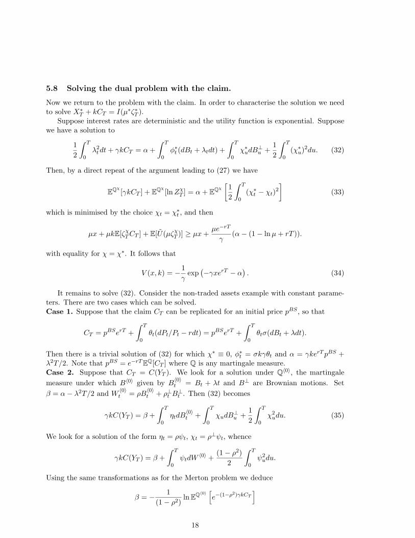
5.8 Solving the dual problem with the claim.

Now we return to the problem with the claim. In order to characterise the solution we needto solve X∗

T + kCT = I(µ∗ζ∗T ).Suppose interest rates are deterministic and the utility function is exponential. Suppose

we have a solution to

12

∫ T

0λ2

tdt+ γkCT = α+∫ T

0φ∗t (dBt + λtdt) +

∫ T

0χ∗udB

⊥u +

12

∫ T

0(χ∗u)2du. (32)

Then, by a direct repeat of the argument leading to (27) we have

EQχ[γkCT ] + EQχ

[lnZχT ] = α+ EQχ

[12

∫ T

0(χ∗t − χt)2

](33)

which is minimised by the choice χt = χ∗t , and then

µx+ µkE[ζχTCT ] + E[U(µζχ

T )] ≥ µx+µe−rT

γ(α− (1− lnµ+ rT )).

with equality for χ = χ∗. It follows that

V (x, k) = −1γ

exp(−γxerT − α

). (34)

It remains to solve (32). Consider the non-traded assets example with constant parame-ters. There are two cases which can be solved.Case 1. Suppose that the claim CT can be replicated for an initial price pBS , so that

CT = pBSerT +∫ T

0θt(dPt/Pt − rdt) = pBSerT +

∫ T

0θtσ(dBt + λdt).

Then there is a trivial solution of (32) for which χ∗ ≡ 0, φ∗t = σkγθt and α = γkerT pBS +λ2T/2. Note that pBS = e−rT EQ[CT ] where Q is any martingale measure.Case 2. Suppose that CT = C(YT ). We look for a solution under Q〈0〉, the martingalemeasure under which B〈0〉 given by B

〈0〉t = Bt + λt and B⊥ are Brownian motions. Set

β = α− λ2T/2 and W 〈0〉t = ρB

〈0〉t + ρ⊥t B

⊥t . Then (32) becomes

γkC(YT ) = β +∫ T

0ηtdB

〈0〉t +

∫ T

0χudB

⊥u +

12

∫ T

0χ2

udu. (35)

We look for a solution of the form ηt = ρψt, χt = ρ⊥ψt, whence

γkC(YT ) = β +∫ T

0ψtdW

〈0〉 +(1− ρ2)

2

∫ T

0ψ2

udu.

Using the same transformations as for the Merton problem we deduce

β = − 1(1− ρ2)

ln EQ〈0〉[e−(1−ρ2)γkCT

]

18

from which it is possible to deduce an expression for α and hence V (x, k).It is possible to combine these two cases to solve the utility indifference pricing problem

for a payoff which is a linear combination of a claim on PT and a claim on YT . SupposeCT = C1(PT ) + C2(YT ). Then

V (x, k) = −1γe−γxerT−γkEQ〈0〉 [C1(PT )]−λ2T/2

(EQ〈0〉

[e−(1−ρ2)γkCT

])1/(1−ρ2).

Finally we use the definition V (x−p(k), k) = V (x, 0) to obtain the following extension of theutility indifference price given in (16):

p(k) = ke−rT EQ〈0〉[C1(PT )]− e−rT

γ(1− ρ2)ln EQ〈0〉

[e−kγ(1−ρ2)C(YT )

]. (36)

Here we have written the first expectation as being under the minimal martingale measure,but of course this component of the price is identical under all choices of martingale measure.

It is an open problem to price a general claim of the form CT = C(PT , YT ), or evento extend the study of claims on YT alone to the case of non-constant correlation. Thefundamental problem is to solve (32) or one of its equivalent variations. Mania et al [57]translate (32) into a backward SDE, and Tehranchi [81] has an interesting approach viathe Holder inequality. It is possible to develop some intuition for the form of the generalsolution by considering the discrete time case, see Smith and Nau [79] and Musiela andZariphopoulou [71], but it is not clear whether this can lead to a closed form expression forthe price such as in (36).

Thus, even in the non-traded assets model with exponential utility, it is difficult to obtainan explicit expression for the utility-indifference price of a contingent claim. In other contextsthe problem is even more difficult, although the general dual expression (21) remains valid. Inthe stochastic volatility context Sircar and Zariphopoulou [78] give a general characterisationof the price of an option on PT and some expansions. In the same class of models, but in theslightly artificial case of an option on the volatility process, Tehranchi [81] and Grasselli andHurd [32] show how to calculate an exact option price.

6 Applications, Extensions and a Literature Review

Utility indifference pricing can be a useful concept of value in any incomplete situation. It hasalready been developed in the context of transactions costs (see below) and for non-tradedassets. Møller [63] uses utility indifference in an insurance context. A number of applicationsare treated in Part 4 of this book. In particular, Chapter 6 deals with indifference pricingof defaultable claims, which is a very new application of these techniques. Chapters 4 and 7treat weather and energy applications of indifference pricing, see also Davis [13] who appliedthe concept of marginal price to weather. We discuss some of these areas in this section andgive references where further details can be found.

6.1 Transactions Costs

Option pricing with transactions costs represents the first area in which utility indifferencepricing was used. Hodges and Neuberger [44] consider an investor endowed with stock, bond,

19

and an option and derive the investor’s optimal investment in stock and bond such that hisexpected utility is maximized in the presence of transactions costs. Under exponential utility,they solve numerically for the optimal hedge in a binomial setting.

The idea was also used in papers of Davis and Norman [14], Davis et al [15], Davisand Zariphopoulou [16] and Constantinides and Zariphopoulou [8], again in the context oftransactions costs. The latter derive a closed form upper bound to the utility indifference priceof a call option. Monoyios [64], [65] considers marginal pricing of options under transactionscosts and computes the option prices numerically.

6.2 Portfolio Constraints

Munk [66] uses utility indifference pricing in the context of portfolio constraints. His con-straints are on the total portfolio amounts, that is, the cash amount in risky stock and theriskless bond. The investor invests in stock and bond, and consumes at rate c in order tomaximize the expected remaining lifetime utility from consumption

sup E∫ ∞

te−β(s−t)U(cs)ds

where utility is power. The investor can also buy or sell units of a European style claim. Inthe special case where the constraint is a non-negative wealth constraint, Merton [60] solvesthe no-option optimal control problem. The option problem is solved numerically by Munk.A second case where the investor faces borrowing constraints is studied numerically.

It is also possible to recast the non-traded assets model as a portfolio constraint problem,where the constraint is that the investor cannot trade on a particular asset. There are anumber of papers written in this vein. First, Kahl et al [51] consider a manager with non-traded stock who can invest in a correlated market asset and bank account, and consume.The manager maximizes expected power utility from consumption and terminal wealth. Kahlet al [51] use utility indifference to value the restricted stock to the manager and solve vianumerical methods. Second, the paper of Tepla [82] considers an investor with exponentialutility who holds some quantity of a non-traded asset in her portfolio. The non-traded payoffis assumed normally distributed, whilst the traded assets are lognormal. Finally, Detempleand Sundaresan [18] treat short sales constraints for American claims.

6.3 Unhedgeable Income Streams

Rather than valuing options or non-traded stock, utility indifference can also be used to valuestreams of income or payments over time where these streams cannot be hedged. In particular,there is a large finance literature on the effect of labour income on asset allocation decisions,see the text of Campbell and Viceira [6]. Labour income is non-traded since individualscannot trade claims to their future wages.

Henderson [36] studies the effect of stochastic income on the optimal investment decisionof an investor who has exponential utility. The income state variable is correlated with a riskytraded asset and the investor maximizes expected utility of terminal wealth where wealth isgenerated by trading in the market and by receiving the stochastic income. Explicit solutionsare found and the effects of income on the optimal portfolio are studied.

20

Munk [67] is a recent paper in a long line looking at an optimal investment and consump-tion problem with stochastic income and power utility over an infinite horizon. He carries outnumerical computations to obtain the value of the non-traded income and optimal portfolio.

6.4 Indifference Pricing for American Options

Davis and Zariphopoulou [16] introduce the notion of American-style utility indifference pricesin the context of transactions costs. Treating the problem of options on non-traded assets,Musiela and Zariphopoulou [69] examine the resulting American utility indifference priceswith exponential utility. In the non-traded asset framework discussed in Section 5.4, thevalue function is shown to be a combination of the classical HJB equation and an obstacleproblem because discretionary stopping is allowed. The buyer’s indifference price solves aquasi-linear variational inequality and in the case where the stock dynamics are lognormal(and the option is only on the non-traded asset), the price can be written as the solution toan optimal stopping problem. The optimal stopping problem involves a non-linear criteriawhich is the same as that appearing in the European case earlier. Assuming interest ratesare zero, the buyer’s price for the American option with payoff C(Yτ ) can be expressed as

pAm(k) = supτ<T

− 1γ(1− ρ2)

ln EQ〈0〉[e−γ(1−ρ2)kC(Yτ )

]Of course, there is no closed form solution to the American option indifference pricing prob-lem, however, Oberman and Zariphopoulou [72] perform some numerical computations forthis problem.

Henderson [37] obtains indifference prices in closed form for perpetual American optionson a non-traded asset under exponential utility. The work was motivated by real options incorporate finance. Real options are options which arise in association with a firm’s decisionmaking. For example, the firm has the option to invest at some time in the future and thisis thought of as a call option on the value of the project with strike equal to the investmentcost. A key feature is that the the underlying project value is often not a traded asset andthus the market is incomplete.

In the framework of Section 5.4 and taking r = 0, with call option payoff at exercise timeτ of (Yτ −K)+, where K is constant, the value function is given by

G(x, y) = supτ

supθu,u≤τ

E[Uτ (Xx,θ

τ + (Yτ −K)+)]

with the appropriate time-consistent utility function Uτ given by

Uτ (x) = −1γe−γxe

12λ2τ .

A non-linear Bellman equation is solved to obtain the value function, and the utility indif-ference value for the call is given by

pperp(1) = sup0≤τ<∞

− 1γ(1− ρ2)

ln EQ〈0〉(e−γ(1−ρ2)(Yτ−K)+)

= − 1γ(1− ρ2)

ln

1− (1− e−γ(1−ρ2)(Y−K))(y

Y

)β(ρ,γ)1

21

whereβ

(ρ,γ)1 = 1− 2(ξ − λρ)

η

and the exercise trigger level Y solves

Y −K =1

γ(1− ρ2)ln

[1 +

γY (1− ρ2)

β(ρ,γ)1

]

Provided β(ρ,γ)1 > 0,

τ = infu : Yu ≥ Y

otherwise, smooth pasting fails and there is no solution. Kadam et al [50] treat the one assetversion of this model, where no trading takes place in a second asset.

6.5 Executive Stock Options

Indifference pricing has been used in valuation of executive stock options. These are typicallycall options on company stock granted to managers as part of their compensation package,see Murphy [68] for an overview of the area and its many important features. The managercannot typically trade in the company stock for insider trading reasons. Usually these optionshave a vesting period inside which the manager cannot sell the options, and after which, theoptions can be sold. However, it is common for models to be constructed assuming theoptions are either European or American for simplicity.

Detemple and Sundaresan [18] apply their binomial model to value executive stock op-tions, using power utility for the manager’s preferences. Henderson [34] applies the continuoustime model with exponential utility to value the options, and also considers the optimal formof the compensation for the company. Her model is one of the only ones to consider the effectof both market and firm-specific risks on executive stock options. The paper of Kadam et al[50] approximates a long dated executive stock option with a perpetual American option.

6.6 Hedging with Additional Instruments

In portfolio optimization problems, it is typically assumed that investors can trade only instocks and bonds. However, it is also reasonable to assume trades in derivative securitiesmay be undertaken, particularly if static rather than dynamic positions are considered. Inan incomplete market situation, the problem of choosing the best static hedge in a derivativecan be solved via utility indifference techniques. This problem is treated in Chapter 5 wherethe optimal static position in a derivative with bounded payoff is found under the assumptionthat the investor has exponential utility.

7 Related approaches

7.1 Super-replication pricing and shortfall hedging

As we mentioned in Section 2.2 on non-Hara utility functions, super-replication pricing andpricing via shortfall hedging can both be interpreted in terms of utility indifference pricingvia a degenerate utility function.

22

The super-replication price can be thought of as an extreme hedging criteria in which theagent is not willing to accept any risk. (The super-replication price is essentially a sell pricefor a claim, and the buy price is given by the sub-replication price.) In the non-traded assetsmodel the super-replication price of a call option on Y is infinite ([46]) whilst in a stochasticvolatility model the super-replication price of a call on X is the cost of buying one unit ofthe underlying ([27]).

A key alternative characterisation of the super-replication price is given in El Karoui andQuenez [20], see also [21, 22], as

supζT

E[ζTCT ]

where the supremum is taken over the set of state-price densities. Thus the super-replicationprice is the sell price under the worst case state-price density.

In shortfall hedging the goal is to minimise the expected losses. This problem has beenconsidered by Follmer and Leukert [23].

7.2 Minimal Distance Martingale Measures

As discussed in Section 5.1 one approach to option pricing in incomplete markets which hasbeen popular in mathematical finance is to fix a martingale measure Q and to use this measurefor pricing. Examples included the mimical martingale measure [25], the variance optimalmeasure [77] or the minimal entropy measure [76, 28]. The equivalent notion in finance is tochoose the market prices of risk on the non-traded assets or Brownian motions.

The issue therefore is to determine a suitable criterion for choosing a martingale measureor market price of risk, or equivalently of choosing the state-price density. One approach isto choose the state-price density which is smallest in an appropriate sense. Given a convexfunction f : R+ 7→ R the idea is to minimise E[f(ζT )] over choices of state-price-density. Aswe have seen, when f(z) = U(µz) this minimisation problem is a key component of the dualapproach.

When interest rates are deterministic and f is homogeneous, this minimisation problemis equivalent to finding the minimal distance martingale measure, the (local) martingalemeasure Q which minimises

E[f(ZT )] (37)

where ZT = dQ/dP. The problem of finding minimal distance measures has been studied bymany authors, but see especially Goll and Ruschendorf [31] who give various characterisationswhich determine the optimal Q in terms of f . Each of the examples listed above can be relatedto a minimal distance measure, for example the minimal entropy measure corresponds to thechoice f(z) = z(ln z − 1).

Once a minimal distance martingale measure Qf has been identified it can be used forpricing in the sense that we can define the option price to be

E[ζfTCT ]

where ζfT is the state-price-density associated with the pricing measure Qf . The resulting

prices are linear in the number of units of claim sold, and as we shall see in the next sectionthey are related to the marginal price of the claim for a utility maximising agent. If theplan is to price options in this way it is important to understand how the prices of options

23

depend on the choice of distance metric. The beginnings of such a study are to be found inHenderson [35] and Henderson et al [40].

Note that in the constant parameter non-traded assets example a simple conditioningargument gives that the minimal martingale measure minimises (37) for all convex f . In thissimple model all minimal distance measures including the minimal entropy measure are equalto the Follmer-Schweizer minimal martingale measure.

7.3 Marginal pricing

Recall that in Section 5.5 on the dual approach we showed that, for positive claims CT andpositive quantities k,

p(k)k

≤ E[ζ0,∗T CT ],

where ζ0,∗T is the state-price density which arises from the optimal solution of the Merton

problem. Furthermore, p(k) is convex in k so that the marginal utility-indifference bid priceexists, where we define the marginal bid price via

D+p := limk↓0

p(k)k

.

Note that we can also define the marginal utility-indifference ask price

D−p := limk↑0

p(k)k

.

A discussion on the necessary and sufficient conditions for marginal prices to exist in a generalsemi-martingale model can be found in Hugonnier et al [47].

By definition we have that V (x− p(k), k) = V (x, 0), and assuming sufficient smoothness,see Davis [11] and Karatzas and Kou [53], we can differentiate to find

−D+p∂V

∂x

∣∣∣∣k=0+

+∂V

∂k

∣∣∣∣k=0+

= 0.

Let Xk,∗T be the optimal target wealth for an agent due to receive k units of the claim CT .

ThenX0,∗T is the solution of the associated Merton problem with zero endowment of the claim,

and U ′(X0,∗T ) = µ∗ζ0,∗

T . Further, since E[ζ0,∗T XT ] = x for any terminal wealth process which

can be financed from initial wealth x, it is reasonable to assume that E[ζ0,∗T (∂Xk,∗

T /∂k)] = 0.Now consider V (x, k) = E[U(Xk,∗

T + kCT )]. We have

∂V

∂k

∣∣∣∣k=0+

= E[U ′

(Xk,∗

T + kCT

)CT

]∣∣∣k=0+

+ E

[U ′

(Xk,∗

T + kCT

) ∂Xk,∗T

∂k

]∣∣∣∣∣k=0+

= µ∗E[ζ0,∗T CT ]

and we have the representation

D+p =µ∗E[ζ0,∗

T CT ]∂V/∂x

(38)

24

This representation is due to Davis [11], at least in the case where D+p and D−p both existand are equal and Davis calls it the fair price. However, see Karatzas and Kou [53] andHobson [42], it is easy to see from the dual representation that ∂V/∂x = µ0,∗ so that (38)simplifies to

D+p = E[ζ0,∗T CT ]. (39)

A key observation is that the quantity ζ0,∗T is the state-price density which arises in the dual

formulation of the solution to the Merton problem. Hence ζ0,∗T is related to a minimal distance

state-price density, and there is a correspondence between marginal utility-indifference pricesand prices derived under a minimal distance martingale measure.

Consider the explicit expressions given for the utility-indifference price for a positiveclaim CT = C(YT ) in the non-traded asset example. We see from (16) and (17) that for bothexponential and power utilities

D+p = e−rT EQ〈0〉[CT ] = E[ζ〈0〉T CT ] (40)

where Q〈0〉 is the minimal martingale measure. Karatzas and Kou [53] show the more generalresult that in the non-traded assets model the marginal bid price is independent of the choiceof utility function and of initial wealth, and given by (40).

Now consider the marginal ask price. For bounded claims the marginal ask price is alsogiven by e−rT EQ〈0〉

[CT ] (see [42]), but this is no longer necessarily the case for unboundedclaims. For example (see Henderson [33]) for Hara utility functions

e−rT EQ〈0〉[CT ] = D+p 6= D−p = ∞.

Thus there are significant gains to be made from differentiating between the marginal bidand ask prices.

7.4 Convex risk measures

Recall the properties of utility-indifference prices we discussed in Section 3: they are non-linear; replicable claims are priced at their Black-Scholes values; prices are monotonic in theclaim; bid prices are concave and sell prices are convex in the claim. Further, for exponentialutility they are independent of the initial wealth.

Coherent risk measures (introduced by Artzner et al [2]) and convex risk measures (Follmerand Schied [24]) were introduced in an attempt to axiomatise measures of risk and to gen-eralise the above properties. In order to be consistent with the rest of this overview we talkabout coherent pricing measures for claims rather than measures of risks. Again, as in thediscussion of super-replication prices, the correspondence is between the price under a riskmeasure and the utility-indifference sell price of a claim.

Let C ∈ C be a contingent claim. Then φ : C 7→ R is a coherent pricing measure if it hasthe properties

Subadditivity φ(C1 + C2) ≤ φ(C1) + φ(C2)Positive homogeneity for λ ≥ 0, φ(λC) = λφ(C)

Monotonicity C1 ≤ C2 =⇒ φ(C1) ≤ φ(C2)Translation invariance φ(C +m) = φ(C) +m

25

For a convex risk measure the subadditivity and positive homogeneity conditions are replacedwith a convexity condition: for µ ∈ (0, 1),

φ(µC1 + (1− µ)C2) ≤ µφ(C1) + (1− µ)φ(C2).

The idea is that φ represents the amount of compensation which an agent would demandin order to agree to sell the claim C (or the size of the reserves he should hold if he hasoutstanding obligations amounting to C).

The key result of [2] is that there is a representation of a coherent pricing measure of theform

φ(C) = supQ∈Q

EQ[C],

where Q is a set of measures. For example the super-replication price is obtained by takingthe set Q to be the set of all martingale measures. Note that a coherent risk measure is linearin the number of claims.

Convex risk measures allow for situations in which the ask price of a claim depends onthe number of units sold. Again (see Chapter 3 of this book for a more complete discussion)there is a representation of a convex pricing measure of the form

φ(C) = supQ∈P

EQ[C]− α(Q)

, (41)

where now P is the set of all probability measures, and α is a penalty function. For example,to recover the super-replication price we may take α(Q) = 0 if Q is a martingale measure,and α(Q) = ∞ otherwise.

A key motivation for the consideration of convex risk measures is that they are a gen-eralisation of the utility-indifference price under exponential utility and zero interest rates.Comparing the expression (21) with k = −1 to (41) we find that the penalty function is ofthe form

α(Q) =1γ

(E[ZT lnZT ]− E[ZE

T lnZET ]

)if Q is a martingale measure, and α(Q) = ∞ otherwise. Here ZE

T is the minimal entropymeasure. Note that like the exponential utility price, but unlike utility-indifference pricesin general, the price under a convex risk measure is independent of the initial wealth of theagent.

8 Conclusion

In a complete frictionless market all risks can be hedged away and a contingent claim has aunique, preference-independent price which is consistent with no-arbitrage. In an incompletemarket it is not possible to hedge away all risk and there is a range of prices which areconsistent with no-arbitrage. In order to specify a particular price for a claim it is necessaryto make assumptions on the risk preferences of agents.

Utility-indifference pricing provides a mechanism for deriving the price of a contingentclaim in an incomplete market. It is a dynamic extension of the static concept of certaintyequivalence from economics. The utility-indifference pricing methodology acknowledges risk,and builds risk preferences into the pricing algorithm via a concave utility function.

26

The utility-indifference price is based on a comparison between optimal behaviours underthe alternative scenarios of buying the claim now and receiving the payoff later, and notbuying the claim. As such it is possible to incorporate a host of features into the model: therisk aversion of the agent, his initial wealth and his prior exposure to non-replicable risk atthe moment he is offered the claim. All of these features will affect the claim price.

The resulting price has many desirable features. The price lies between the upper andlower limits consistent with no-arbitrage (and these limits can be attained by an appropriatechoice of utility function), and it reduces to the complete market price for replicable claims.Moreover, implicit in the calculation of the utility-indifference price is the construction of anoptimal hedge.

The difficulties with the utility-indifference paradigm are that firstly, in order to initiatethe process it is necessary to determine the agent’s utility function, a notoriously difficulttask, and secondly, even when these preferences have been specified it is very difficult to solvethe optimisation problems which arise. Analytic formula for contingent claims can be derivedin only a few special cases. Such formula are easiest to derive under exponential, logarithmicor quadratic utility, but financial economists prefer to use power utility. (Estimates of theco-efficient of relative risk aversion R vary in the range 4 to 10, see Cochrane [7], whereasexponential, logarithmic and quadratic utility correspond to R = ∞, R = 1 and R = −1respectively.)

The use of duality theory has led to several recent advances in the characterisation ofoptimal behaviour of utility maximising agents, but there is a need for more explicit solutionsto be derived, and for the parallels with other incomplete-market pricing methodologies whichwe discussed in this overview to be developed and extended. Together with the translationof the utility-indifference approach to new problems and frameworks, these are the majorthemes of this book, which contains some of the latest developments in the subject.

27

References

[1] K. Arrow. Essays in the Theory of Risk Bearing. North-Holland, Amsterdam, 1970.

[2] P. Artzner, F. Delbaen, J.M. Eber, and D. Heath. Coherent measures of risk. Mathe-matical Finance, 9:203–228, 1999.

[3] D. Becherer. Rational hedging and valuation with utility-based preferences. PhD thesis,Technical University of Berlin, 2001.

[4] D. Bernoulli. Specimen theoriae novae de mensura sortis. Commentarii AcademiaeSientiarum Imperialis Petropolitanae, (and translated in Econometrica), 5 (and 22):175–192 and 23–56, 1738 (and 1954).

[5] N. Branger. Pricing derivative securities using cross entropy - an economic analysis.International Journal of Theoretical and Applied Finance, 7:63–82, 2004.

[6] J.Y. Campbell and L.M. Viceira. Strategic Asset Allocation: Portfolio Choice for LongTerm Investors. OUP, 2002.

[7] J.H. Cochrane. Asset Pricing. Princeton University Press, 2001.

[8] G.M. Constantinides and T. Zariphopoulou. Bounds on prices of contingent claims inan intertemporal economy with proportional transactions costs and general preferences.Finance and Stochastics, 3:345–369, 1999.

[9] T.E. Copeland and J.F. Weston. Financial Theory and Corporate Policy. Addison-Wesley, New York, 1992.

[10] J. Cvitanic, W. Schachermayer, and H. Wang. Utility maximisation in incomplete mar-kets with random endowment. Finance and Stochastics, 5(2):259–272, 2001.

[11] M.H.A. Davis. Option pricing in incomplete markets. In M.A.H. Dempster and S.R.Pliska, editors, Mathematics of Derivative Securities, pages 216–227. Cambridge Univer-sity Press, Cambridge, 1997.

[12] M.H.A. Davis. Option valuation and basis risk. In T.E. Djaferis and L.C. Shick, editors,System Theory: Modelling, Analysis and Control. Academic Publishers, 1999.

[13] M.H.A. Davis. Pricing weather derivatives by marginal value. Quantitative Finance,1:1–4, 2001.

[14] M.H.A Davis and A.R. Norman. Portfolio selection with transactions costs. Mathematicsof Operations Research, 15:676–713, 1990.

[15] M.H.A Davis, V.G. Panas, and T. Zariphopoulou. European option pricing with trans-actions costs. SIAM Journal on Control and Optimization, 31:470–493, 1993.

[16] M.H.A. Davis and T. Zariphopoulou. American options and transaction fees. In Math-ematical Finance IMA Volumes in Mathematics and its Applications. Springer-Verlag,1995.

28

[17] F. Delbaen, P. Grandits, T. Rheinlander, D. Sampieri, M. Schweizer, and Ch. Stricker.Exponential hedging and entropic penalties. Mathematical Finance, 12:99–124, 2002.

[18] J. Detemple and S. Sundaresan. Nontraded asset valuation with portfolio constraints: abinomial approach. Review of Financial Studies, 12:835–872, 1999.

[19] D. Duffie and H.R. Richardson. Mean-variance hedging in continuous time. Annals ofApplied Probability, 1:1–15, 1991.

[20] N. El-Karoui and M.C. Quenez. Dynamic programming and pricing of contingent claimsin an incomplete market. SIAM Journal of Control and Optimization, 33:29–66, 1995.

[21] H. Follmer and Y. Kabanov. Optional decomposition and lagrange multipliers. Financeand Stochastics, 2:69–81, 1998.

[22] H. Follmer and D. Kramkov. Optional decompositions under constraints. ProbabilityTheory and Related Fields, 109:1–25, 1997.

[23] H. Follmer and P. Leukert. Efficient hedging: cost versus shortfall risk. Finance andStochastics, pages –, 1999.

[24] H. Follmer and A. Schied. Convex measures of risk and trading constraints. Financeand Stochastics, 6:429–447, 2002.

[25] H. Follmer and M. Schweizer. Hedging of contingent claims under incomplete infor-mation. In M.H.A. Davis and R.J. Elliott, editors, Applied Stochastic Analysis, pages389–414. Gordon and Breach, London, 1990.

[26] R. Frey. Derivative asset analysis in models with level-dependent and stochastic volatility.CWI Quarterly, 10:1–34, 1997.

[27] R. Frey and C. Sin. Bounds on european option prices under stochastic volatility. Math-ematical Finance, 9:97–116, 1999.

[28] M. Frittelli. The minimal entropy martingale measure and the valuation problem inincomplete markets. Mathematical Finance, 10(1):39–52, 2000.

[29] H. Geman, N. El Karoui, and J-C Rochet. Changes of numeraire, changes of probabilityand option pricing. Journal of Applied Probability, 32:443–458, 1995.

[30] H.U. Gerber. An introduction to mathematical risk theory. Huebner Foundation forInsurance Education, 1979.

[31] T. Goll and L. Ruschendorf. Minimax and minimal distance martingale measures andtheir relationship to portfolio optimisation. Finance and Stochastics, 5:557–581, 2001.

[32] M.R. Grasselli and T.R. Hurd. Indifference pricing and hedging in stochastic volatilitymodels. Technical report, McMaster University, 2004.

[33] V. Henderson. Valuation of claims on non-traded assets using utility maximization.Mathematical Finance, 12(4):351–373, 2002.

29

[34] V. Henderson. The impact of the market portfolio on the valuation, incentives andoptimality of executive stock options. To appear, 2003.

[35] V. Henderson. Analytical comparisons of option prices in stochastic volatility models.Mathematical Finance, 2004. To appear.

[36] V. Henderson. Explicit solutions to an optimal portfolio choice problem with stochasticincome. Journal of Economic Dynamics and Control, 2004. To appear.

[37] V. Henderson. Valuing the option to invest in an incomplete market. Technical report,Princeton University, 2004.

[38] V. Henderson and D. Hobson. Real options with constant relative risk aversion. Journalof Economic Dynamics and Control, 27:329–355, 2002.

[39] V. Henderson and D. Hobson. Substitute hedging. RISK, 15(5):71–75, 2002.

[40] V. Henderson, D. Hobson, S. Howison, and T. Kluge. A comparison of q-optimal optionprices in a stochastic volatility model with correlation. Technical report, University ofOxford, 2003.

[41] S.L. Heston. A closed-form solution for options with stochastic volatility and applicationsto bond and currency options. Review of Financial Studies, 6:327–343, 1993.

[42] D.G. Hobson. Real options, non-traded assets and utility indifference prices. Technicalreport, University of Bath, 2003.

[43] D.G. Hobson. Stochastic volatility, correlation and the q-optimal measure. MathematicalFinance, 2004. To appear.

[44] S. Hodges and A. Neuberger. Optimal replication of contingent claims under transactionscosts. Review of Futures Markets, 8:222–239, 1989.

[45] C. Huang and R.H Litzenberger. Foundations for Financial Economics. North-Holland,New York, 1988.

[46] F. Hubalek and W. Schachermayer. The limitations of no-arbitrage arguments for realoptions. International Journal of Theoretical and Applied Finance, 4:361–373, 2001.

[47] J. Hugonnier, D. Kramkov, and W. Schachermayer. On utility based pricing of contingentclaims in incomplete markets. Mathematical Finance, 2004. to appear.

[48] J. Hull and A. White. The pricing of options on assets with stochastic volatilities.Journal of Finance, 42(2):281–300, 1987.

[49] W.S. Jevons. The Theory of Political Economy. reprinted Pelican Books, London, 1970,1871.

[50] A. Kadam, P. Lakner, and A. Srinivasan. Executive stock options: value to the executiveand cost to the firm’. Technical report, Preprint, 2003.

30

[51] M. Kahl, J. Liu, and F. Longstaff. Paper millionaires: How valuable is stock to astockholder who is restricted from selling it ? Journal of Financial Economics, 67:385–410, 2003.

[52] J. Kallsen. Derivative pricing based on local utility maximisation. Finance and Stochas-tics, 6:115–140, 2002.

[53] I. Karatzas and S. Kou. On the pricing of contingent claims under constraints. Annalsof Applied Probability, 6(2):321–369, 1996.

[54] I. Karatzas, J.P. Lehoczky, S.E. Shreve, and G-L. Xu. Martingale and duality meth-ods for utility maximisation in an incomplete market. SIAM Journal of Control andOptimisation, 29:702–730, 1991.

[55] M. Kobylanski. Backward stochastic differential equations and partial differential equa-tions with quadratic growth. Annals of Probability, 28:558–602, 2000.

[56] D. Kramkov and W. Schachermayer. The asymptotic elasticity of utility functions andoptimal investment in incomplete markets. Annals of Applied Probability, 9(3):904–950,1999.

[57] M. Mania, M. Santacroce, and R. Tevzadze. A semimartingale bsde related to theminimal entropy martingale measure. Finance and Stochastics, 7:385–402, 2003.

[58] W. Margrabe. The value of an option to exchange one asset for another. Journal ofFinance, 33:177–186, 1978.

[59] A. Mas-Colell, M.D. Whinston, and J.R. Green. Microeconomic Theory. OUP, 1995.

[60] R. C. Merton. Lifetime portfolio selection under uncertainty: the continuous-time case.Rev. Econom. Statist., 51:247–257, 1969.

[61] R. C. Merton. Optimum consumption and portfolio rules in a continuous-time model.J. Economic Theory, 3:373–413, 1971.

[62] R.C. Merton. Continuous Time Finance. Basil Blackwell Ltd UK, 1992.

[63] T. Møller. Indifference pricing of insurance contracts in a product space model. Financeand Stochastics, 7:197–217, 2003.

[64] M. Monoyios. Efficient option pricing with transactions costs. Journal of ComputationalFinance, 7(1), 2003.

[65] M. Monoyios. Option pricing with transactions costs using a markov chain approxima-tion. Journal of Economic Dynamics and Control, 28(5):889–913, 2004.

[66] C. Munk. The valuation of contingent claims under portfolio constraints: reservationbuying and selling prices. European Finance Review, 3:347–388, 1999.

[67] C. Munk. Optimal consumption/investment policies with undiversifiable income riskand liquidity constraints. Journal of Economic Dynamics and Control, 24:1315–1343,2000.

31

[68] K. Murphy. Executive compensation. In O. Ashenfelter and D. Card, editors, Handbookof Labor Economics. North-Holland, 1999.

[69] M. Musiela and T. Zariphopoulou. Indifference prices of early exercise claims. Technicalreport, University of Texas, Austin, 2003.

[70] M. Musiela and T. Zariphopoulou. An example of indifference prices under exponentialpreferences. Finance and Stochastics, 8(2):229–239, 2004.

[71] M. Musiela and T. Zariphopoulou. A valuation algorithm for indifference prices inincomplete markets. Finance and Stochastics, 8(3):399–414, 2004.

[72] A. Oberman and T. Zariphopoulou. Pricing early exercise contracts in incomplete mar-kets. Computational Management Science, 2003. To appear.

[73] M. P. Owen. Utility based optimal hedging in incomplete markets. The Annals of AppliedProbability, 12(2):691–709, 2002.

[74] J. Pratt. Risk aversion in the small and in the large. Econometrica, 32:122–136, 1964.

[75] T. Rheinlander. An entropy approach to the stein/stein model with correlation. Tech-nical report, ETH Zurich, 2002.

[76] R. Rouge and N. El Karoui. Pricing via utility maximization and entropy. MathematicalFinance, 10:259–276, 2000.

[77] M. Schweizer. Approximation pricing and the variance optimal martingale measure.Annals of Probability, 24:206–236, 1996.

[78] R. Sircar and T. Zariphopoulou. Bounds and asymptotic approximations for utilityprices when volatility is random. SIAM J. Control & Optimization, 2004. To appear.

[79] J.E. Smith and R.F. Nau. Valuing risky projects: option pricing theory and analysis.Management Science, 41(5):795–816, 1995.

[80] E.M. Stein and J.C. Stein. Stock-price distributions with stochastic volatility: an ana-lytic approach. Review Financial Studies, 4:727–752, 1991.

[81] M. Tehranchi. Explicit solution of some utility maximization problems in incompletemarkets. Stochastic Proc. and Appl., pages 1568–1590, October 2004.

[82] L. Tepla. Optimal hedging and valuation of non-traded assets. European Finance Review,4:221–251, 2000.

[83] T. Zariphopoulou. A solution approach to valuation with unhedgeable risks. Finance &Stochastics, 5:61–82, 2001.

32