Using Ancestral State ReconstructionMethods for OnomasiologicalReconstruction in Multilingual Word Lists

Gerhard JägerInstitute of LinguisticsTübingen, Germanygerhard.jaeger@uni-tuebingen.de.Johann-Mattis ListDepartment for Linguistic andCultural EvolutionMax Planck Institute for theScience of Human History, Jenamattis.list@shh.mpg.de

Current efforts in computational historical linguistics are predominantly concerned withphylogenetic inference. Methods for ancestral state reconstruction have only been appliedsporadically. In contrast to phylogenetic algorithms, automatic reconstruction methodspresuppose phylogenetic information in order to explain what has evolved when andwhere. Here we report a pilot study exploring how well automatic methods for ancestralstate reconstruction perform in the task of onomasiological reconstruction in multilingualword lists, where algorithms are used to infer how the words evolved along a givenphylogeny, and reconstruct which cognate classes were used to express a given meaningin the ancestral languages. Comparing three different methods, Maximum Parsimony,Minimal Lateral Networks, and Maximum Likelihood on three different test sets (Indo-European, Austronesian, Chinese) using binary and multi-state coding of the dataas well as single and sampled phylogenies, we find that Maximum Likelihood largelyoutperforms the other methods. At the same time, however, the general performancewas disappointingly low, ranging between 0.66 (Chinese) and 0.79 (Austronesian) forthe F-Scores. A closer linguistic evaluation of the reconstructions proposed by the bestmethod and the reconstructions given in the gold standards revealed that the majorityof the cases where the algorithms failed can be attributed to problems of independentsemantic shift (homoplasy), to morphological processes in lexical change, and to wrongreconstructions in the independently created test sets that we employed.

ancestral state reconstruction – lexical reconstruction – computational historicallinguistics – phylogenetic methods

1 Introduction

Phylogenetic reconstruction methods are crucial for recent quantitative approaches inhistorical linguistics. While many scholars remain skeptical regarding the potentialof methods for automatic sequence comparison, phylogenetic reconstruction, be it ofnetworks using the popular SplitsTree software (Huson, 1998), or family trees, usingdistance- (Sokal and Michener, 1958: Saitou and Nei, 1987) or character-based approaches(Edwards and Cavalli-Sforza, 1964: Fitch, 1971: Ronquist et al., 2012: Bouckaert et al.,2014), has entered the mainstream of historical linguistics. This is reflected in a multitudeof publications and applications on different language families, from Ainu (Lee andHasegawa, 2013) and Australian (Bowern and Atkinson, 2012) to Semitic (Kitchen et al.,2009) and Chinese (Ben Hamed and Wang, 2006). There is also a growing interest in theimplications of phylogenetic analyses for historical linguistics, as can be seen from theheated debate about the dating of Indo-European (Gray and Atkinson, 2003: Atkinsonand Gray, 2006: Bouckaert et al., 2014: Chang et al., 2015), and the recent attempts tosearch for deep genetic signals in the languages of the world (Pagel et al., 2013: Jäger,2015).

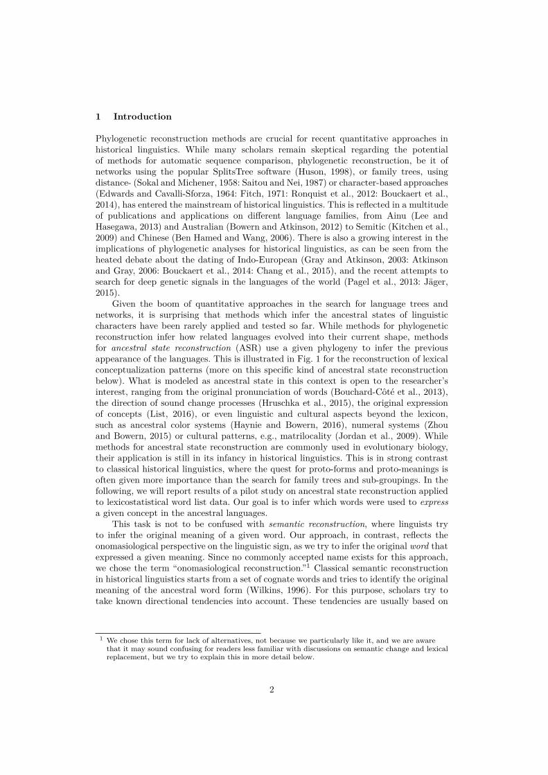
Given the boom of quantitative approaches in the search for language trees andnetworks, it is surprising that methods which infer the ancestral states of linguisticcharacters have been rarely applied and tested so far. While methods for phylogeneticreconstruction infer how related languages evolved into their current shape, methodsfor ancestral state reconstruction (ASR) use a given phylogeny to infer the previousappearance of the languages. This is illustrated in Fig. 1 for the reconstruction of lexicalconceptualization patterns (more on this specific kind of ancestral state reconstructionbelow). What is modeled as ancestral state in this context is open to the researcher’sinterest, ranging from the original pronunciation of words (Bouchard-Côté et al., 2013),the direction of sound change processes (Hruschka et al., 2015), the original expressionof concepts (List, 2016), or even linguistic and cultural aspects beyond the lexicon,such as ancestral color systems (Haynie and Bowern, 2016), numeral systems (Zhouand Bowern, 2015) or cultural patterns, e.g., matrilocality (Jordan et al., 2009). Whilemethods for ancestral state reconstruction are commonly used in evolutionary biology,their application is still in its infancy in historical linguistics. This is in strong contrastto classical historical linguistics, where the quest for proto-forms and proto-meanings isoften given more importance than the search for family trees and sub-groupings. In thefollowing, we will report results of a pilot study on ancestral state reconstruction appliedto lexicostatistical word list data. Our goal is to infer which words were used to expressa given concept in the ancestral languages.

This task is not to be confused with semantic reconstruction, where linguists tryto infer the original meaning of a given word. Our approach, in contrast, reflects theonomasiological perspective on the linguistic sign, as we try to infer the original word thatexpressed a given meaning. Since no commonly accepted name exists for this approach,we chose the term “onomasiological reconstruction.”1 Classical semantic reconstructionin historical linguistics starts from a set of cognate words and tries to identify the originalmeaning of the ancestral word form (Wilkins, 1996). For this purpose, scholars try totake known directional tendencies into account. These tendencies are usually based on

1 We chose this term for lack of alternatives, not because we particularly like it, and we are awarethat it may sound confusing for readers less familiar with discussions on semantic change and lexicalreplacement, but we try to explain this in more detail below.

2

the author’s intuition, despite recent attempts to formalize and quantify the evidence(Urban, 2011). Following the classical distinction between semasiology and onomasiologyin semantics, the former dealing with ‘the meaning of individual linguistic expressions’(Bussmann, 1996:1050), and the latter dealing with the question of how certain conceptsare expressed (ibd.:834), semantic reconstruction is a semasiological approach to lexicalchange, as scholars start from the meaning of several lexemes in order to identify themeaning of the proto-form and its later development.

Kopf"head"

kop"head"

head"head"

tête"head"

testa"head"

cap"head"

*kop"head"

*haubud-"head"

testa"head"

caput"head"

*kaput-"head"

Kopf"head"

kop"head"

head"head"

tête"head"

testa"head"

cap"head"

"head"

?

?

?

?

?

Figure 1Ancestral state reconstruction: The graphic illustrates the key idea of ancestral statereconstruction. Given six words in genetically related languages, we inquire how these wordsevolved into their current shape. Having inferred a phylogeny of the languages as shown on theleft of the figure, ancestral state reconstruction methods use this phylogeny to find the bestway to explain how the six words have evolved along the tree, thereby proposing ancestralstates of all words under investigation. The advantage of this procedure is that we canimmediately identify not only the original nature of the characters we investigate, but also thechanges they were subject to. Ancestral state reconstruction may thus yield important insightsinto historical processes, including sound change and lexical replacement.

Instead of investigating lexical change from the semasiological perspective, one couldalso ask which of several possible word forms was used to denote a certain meaning in agiven proto-language. This task is to some degree similar to proper semantic reconstruc-tion, as it deals with the question of which meaning was attached to a given linguisticform. The approach, however, is onomasiological, as we start from the concept andsearch for the “name” that was attached to it. Onomasiological semantic reconstruction,the reconstruction of former expressions, has been largely ignored in classical semanticreconstruction.2 This is unfortunate, since the onomasiological perspective may offerinteresting insights into lexical change. Given that we are dealing with two perspectiveson the same phenomenon, the onomasiological viewpoint may increase the evidence forsemantic reconstruction.

This is partially reflected in the “topological principle in semantic [i.e. onomasio-logical, GJ and JML] reconstruction” proposed by Kassian et al. (2015). This principleuses phylogenies to support claims about the reconstruction of ancestral expressions inhistorical linguistics, trying to choose the ‘most economic scenario’ (ibd.:305) involving

2 Notable exceptions include work by S. Starostin and colleagues, compare, for example, Starostin(2016).

3

the least amount of semantic shifts. By adhering to the onomasiological perspective andmodifying our basic data, we can model the problem of onomasiological reconstructionas an ancestral state reconstruction task, thereby providing a more formal treatmentof the topological principle. In this task, we (1) start from a multilingual word lists inwhich a set of concepts has been translated into a set of languages (a classical “Swadeshlist” or lexicostatistic word list; Swadesh, 1955), (2) determine a plausible phylogeny forthe languages under investigation, and (3) use ancestral state reconstruction methodsto determine which word forms were most likely used to express the concepts in theancestral languages in the tree. This approach yields an analysis as the one shown in Fig.1.

Although we think that such an analysis has many advantages over the manualapplication of the topological principle in onomasiological reconstruction employed byKassian et al. (2015), we should make very clear at this point that our reformulation of theproblem as an ancestral state reconstruction task also bears certain shortcomings. First,since ancestral state reconstruction models character by character independently fromeach other, our approach relies on identical meanings only and cannot handle semanticfields with fine-grained meaning distinctions. This is a clear disadvantage compared toqualitative analyses, but given that models always simplify reality, and that neither algo-rithms nor datasets for testing and training are available for the extended task, we think itis justified to test how close the available ancestral state reconstruction methods come tohuman judgments. Second, our phylogenetic approach to onomasiological reconstructiondoes not answer any questions regarding semantic change, as we can only state whichwords are likely to have been used to express certain concepts in ancestral languages. Thisresults clearly from the data and our phylogenetic approach, as mentioned before, and it isan obvious shortcoming of our approach. However, since the phylogenetic onomasiologicalreconstruction provides us with concrete hypotheses regarding the meaning of a givenword on a given node in the tree, we can take these findings as a starting point to furtherinvestigate how words changed their meaning afterwards. By providing a formal anddata-driven way to apply the topological principle, we can certainly contribute to thebroader tasks of semantic and onomasiological reconstruction in historical linguistics. Asa third point, we should not forget that our method suffers from the typical shortcomingsof all data-driven disciplines, namely the shortcomings resulting from erroneous dataassembly, especially erroneous cognate judgments, such as undetected borrowings (Holm,2007) and inaccurate translations of the basic concepts (Geisler and List, 2010) whichare investigated in all approaches based on lexicostatistical data. The risk that errors inthe data have an influence on the inferences made by the methods is obvious and clear.In order to make sure that we evaluate the full potential of phylogenetic methods forancestral state reconstruction, we therefore provide an exhaustive error analysis not onlyfor the inferences made in our tests, but also for the data we used for testing.

In the following, we illustrate how ancestral state reconstruction methods can beused to approximate onomasiological reconstruction in multilingual word lists. We testthe methods on three publicly available datasets from three different language familiesand compare the results against experts’ assessments.

4

2 Materials and methods

2.1 Materials2.1.1 Gold standardIn order to test available methods for ancestral state reconstruction, we assembled lexicalcognacy data from three publicly available sources, offering data on three differentlanguage families of varying size:

1. Indo-European languages, as reflected in the Indo-European lexical cognacydatabase (IELex; Dunn, 2012, accessed on September 5, 2016),

2. Austronesian languages, as reflected in the Austronesian Basic VocabularyDatabase (ABVD; Greenhill et al., 2008, accessed on December 2, 2015),and

3. Chinese dialect varieties, as reflected in the Basic Words of ChineseDialects (BCD; Wang, 2004, provided in List, 2016).

All datasets are originally classical word lists as used in standard approaches to phylo-genetic reconstruction: They contain a certain number of concepts which are translatedinto the target languages and then annotated for cognacy. In order to be applicable asa test set for our analysis, the datasets further need to list proto-forms of the supposedancestral language of all languages in the sample. All data we used for our studies isavailable from the supplementary material.

The BCD database was used by Ben Hamed and Wang (2006) and is no longeraccessible via its original URL, but it has been included in List (2015) and later revisedin List (2016). It comprises data on 200 basic concepts (a modified form of the conceptlist by Swadesh, 1952) translated into 23 Chinese dialect varieties. Additionally, Wang(2004) lists 230 translations in Old Chinese for 197 of the 200 concepts. Since Old Chineseis the supposed ancestor of all Chinese dialects, this data qualifies as a gold standard forour experiment on ancestral state reconstruction. We should, however, bear in mind thatthe relationship between Old Chinese, as a variety spoken some time between 800 and200 BC, and the most recent common ancestor of all Chinese dialects, spoken between200 and 400 CE, is a remote one. We will discuss this problem in more detail in ourlinguistic evaluation of the results in section 4. Given that many languages containmultiple synonyms for the same concept, the data, including Old Chinese, comprises5,437 words, which can be clustered into 1,576 classes of cognate words; 980 of these are“singletons,” that is, they comprise classes containing only one single element. Due tothe large time span between Old Chinese and the most recent common ancestor of allChinese dialects, not all Old Chinese forms are technically reconstructible from the data,as they reflect words that have been lost in all dialects. As a result, we were left with 144reconstructible concepts for which at least one dialect retains an ancestral form attestedin Old Chinese.

For the IELex data,3 we used all languages and dialects except those marked as“Legacy” and two creole languages (Sranan and French Creole Dominica, as lexicalchange arguably underlies different patterns under creolization than it does in normal

3 IELex is currently being thoroughly revised as part of the Cognates in the Basic Lexicon (COBL)project, but since this data has not yet been publicly released, we were forced to use the IELex datawhich we retrieved from ielex.mpi.nl.

5

language change). This left us with 134 languages and dialects, including 31 ancientlanguages (Ancient Greek, Avestan, Classical Armenian, Gaulish, Gothic, Hittite, Latin,Luvian, Lycian, Middle Breton, Middle Cornish, Mycenaean Greek, Old Persian, OldPrussian, Old Church Slavonic, Old Gutnish, Old Norse, Old Swedish, Old High German,Old English, Old Irish, Old Welsh, Old Cornish, Old Breton, Oscan, Palaic, Pali,Tocharian A, Tocharian B, Umbrian, Vedic Sanskrit). The data contain translationsof 208 concepts into those languages and dialects (often including several synonymousexpressions for the same concept from the same language). Most entries are assigned acognate class label. We only used entries containing an unambiguous class label, which leftus with 26,524 entries from 4,352 cognate classes. IELex also contains 167 reconstructedentries (for 135 concepts) for Proto-Indo-European. These reconstructions were used asgold standard to evaluate the automatically inferred reconstructions.

ABVD contains data from a total of 697 Austronesian languages and dialects. Weselected a subset of 349 languages (all taken from the 400-language sample used in Grayet al., 2009), each having a different ISO code which is also covered in the Glottologdatabase (Hammarström et al., 2015). ABVD covers 210 concepts, with a total of 44,983entries from 7,727 cognate classes for our 349-language sample. It also contains 170reconstructions for Proto-Austronesian (each denoting a different concept) includingcognate-class assignments. An overview of the data used is given in Table 1.

Dataset Languages Concepts Cognate Classes Singletons WordsIELex 134 207 (135 reconstructible) 4,352 1,434 singletons 26,524ABVD 349 210 (170 reconstructible) 7,727 2,671 singletons 44,983BCD 24 200 (144 reconstructible) 1.576 980 singletons 5,437

Table 1Datasets used for ancestral state reconstruction. “Reconstructible” states in the columnshowing the number of concepts refer to the amount of concepts in which the proto-form isreflected in at least one of the descendant languages. “Singletons” refer to cognate sets withonly one reflex, which are not informative for the purpose of certain methods of ancestral statereconstruction, like the MLN approach, and therefore excluded from the analysis.

2.2 Methods2.2.1 Reference phylogeniesAll ASR methods in our test (except the baseline) rely on phylogenetic information wheninferring ancestral states, albeit to a different degree. Some methods operate on a singletree topology only, while other methods also use branch lengths information or requirea sample of trees to take phylogenetic uncertainty into account. To infer those trees, wearranged the cognacy information for each data set into a presence-absence matrix. Sucha data structure is a table with languages as rows and cognate classes occurring withinthe data set as columns. A cell for language l and cognate class cc for concept c has entry

• 1 if cc occurs among the expressions for c in l,

• 0 if the data contain expressions for c in l, but none of them belongs to cc,and

• undefined if l does not contain any expressions for c.

6

Bayesian phylogenetic inference was performed on these matrices. For each data set,tree search was constrained by prior information derived from the findings of traditionalhistorical linguistics. More specifically, we used the following prior information:

• IELex. We used 14 topological constraints (see Fig. 2), age constraints forthe 31 ancient languages, and age constraints for 11 of the 14 topologicalconstraints.The age constraints for Middle Breton, Middle Cornish, Mycenaean Greek,Old Breton, Old Cornish, Old Welsh, and Palaic are based on informationfrom Multitree (The LINGUIST List, 2014, accessed on October 14, 2016).The age constraint for Pali is based on information from EncyclopaediaBritannica (2010, accessed on October 14, 2016). The constraints for OldGutnish are taken from Wessen (1968) and those for Old Swedish and OldHigh German from Campbell and King (2013). All other age constraints arederived from the Supplementary Information of Bouckaert et al. (2012).

Latin

Gaulish

Gothic

0,999

0,186

0,464

0,942

0,767

0,834

0,752

0,472

0,965

0,393

0,676

0,985

0,967

0,992

0,883

0,578

0,12

AnatolianTocharic

GreekArmenian

Indic

Nuristani

Iranian

Baltic

Slavic

Albanian

French/Iberian

RomanceItalic

West Germanic

North Germanic

Goidelic

Brythonic

Nuclear Indo-European

Northwest Germanic

Celtic

Balto-Slavic

Indo-Iranian

Figure 2Maximum Clade Credibility tree for IELex (schematic). Topological constraints are indicatedby red circles. Numbers at intermediate nodes indicate posterior probabilities (only shown if< 1).

• ABVD. We only considered trees consistent with the Glottolog expertclassification (Hammarström et al., 2015). This amounts to 213 topologicalconstraints.

7

• BDC. We only considered trees consistent with the expert classificationfrom Sagart (2011). This amounts to 20 topological constraints.

Analyses were carried out using the MrBayes software (Ronquist et al., 2012).Likelihoods were computed using ascertainment bias correction for all-absent charactersand assuming Gamma-distributed rates (with 4 Gamma categories). Regarding the treeprior, we assumed a relaxed molecular clock model (more specifically, the IndependentGamma Rates model (cf. Lepage et al., 2007), with an exponential distribution with rate200 as prior distribution for the variance of rate variation). Furthermore we assumeda birth-death model (Yang and Rannala, 1997) and random sampling of taxa with asampling probability of 0.2. For all other parameters of the prior distribution, the defaultsoffered by the software were used.4

For each dataset, a maximum clade credibility tree was identified as the referencetree (using the software TreeAnnotator, retrieved on September 13, 2016; part of thesoftware suite Beast, cf. Bouckaert et al., 2014). Additionally, 100 trees were sampledfrom the posterior distribution for each dataset and used as tree sample for ASR.

2.2.2 Ancestral state reconstructionFor our study, we tested three different established algorithms, namely (1) MaximumParsimony (MP) reconstruction using the Sankoff algorithm (Sankoff, 1975), (2) theminimal lateral network (MLN) approach (Dagan et al., 2008) as a variant of MaximumParsimony in which parsimony weights are selected with the help of the vocabulary sizecriterion (List et al., 2014b c), and (3) Maximum Likelihood (ML) reconstruction asimplemented in the software BayesTraits (Pagel and Meade, 2014). These algorithms aredescribed in detail below.

We tested two different ways to arrange cognacy information as character matrices:

• Multistate characters. Each concept is treated as a character. The valueof a character for a given language is the cognate class label of thatlanguage’s expression for the corresponding concept. If the data containseveral non-cognate synonymous expressions, the language is treated aspolymorphic for that character. If the data do not contain an expression fora given concept and a given language, the corresponding character value isundefined.

• Binary characters. Each cognate class label that occurs among thedocumented languages of a dataset is a character. Possible values are 1 (alanguage contains an expression from that cognate class), 0 (a languagedoes not contain an exponent of that cognate class, but other expressionsfor the corresponding concept are documented) or undefined (the data donot contain an expression for the concept from the language in question).

All three algorithms rely on a reference phylogeny to infer ancestral states. To testthe impact of phylogenetic uncertainty, we performed ASR both on the reference tree

4 These defaults are: uniform distribution over equilibrium state frequencies; standard exponentialdistribution as prior for the shape parameter α of the Gamma distribution modeling rate variation;standard exponential distribution as prior over the tree age, measured in expected number ofmutations per character.

8

and on the tree sample for all three algorithms. The procedures are now presented foreach algorithm in turn.

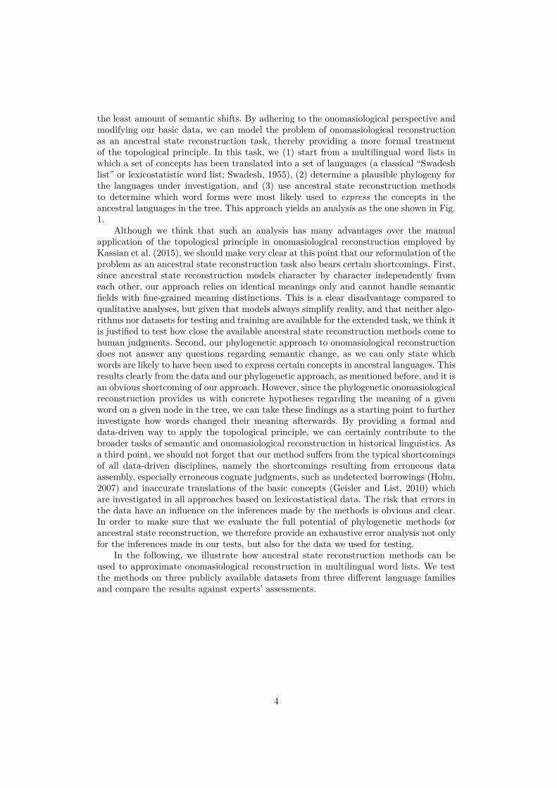
Maximum Parsimony (MP). A complete scenario for a character is a phylogenetic treewhere all nodes are labeled with some character value. For illustration, three scenariosare shown in Fig. 3. The parsimony score of a scenario is the number of mutations, i.e.,of branches where the mother node and the daughter node carry different labels. Nowsuppose only the labels at the leaves of the tree are given. The parsimony score of sucha partial scenario is the minimal parsimony score of any complete scenario consistentwith the given leaf labels. In the example in Fig. 3, this value would be 2. The ASRfor the root of the tree would be the root label of the complete scenario giving rise tothis minimal parsimony score. If several complete scenarios with different root labels giverise to the same minimal score, all their root labels are possible ASRs. This logic can begeneralized to weighted parsimony. In this framework, each mutation from a state at themother node to the state at the daughter node of a tree has a certain penalty, and thesepenalties may differ for different types of mutations. The overall parsimony score of acomplete scenario is the sum of all penalties for all mutations in this scenario.5

A C C

B

A B B

A

BB

C

Parsimony = 2

A C CA B B

A

B

C

Parsimony = 3A

A

A C CA B B

AC

Parsimony = 3

A

C

C

Figure 3Complete character scenarios. Mutations are indicated by yellow stars.

The Sankoff algorithm is an efficient method to compute the parsimony score andthe root ASR for a partial scenario. It works as follows. Let states be the ordered set ofpossible states of the character in question, and let n be the cardinality of this set. Foreach pair of states i, j, w(i, j) is the penalty for a mutation from statesi to statesj .

5 There is a variant of MP called Dollo parsimony (Le Quesne, 1974: Farris, 1977) which is primafacie well-suited for modeling cognate class evolution. Dollo parsimony rests on the assumption thatcomplex characters evolve only once, while they may be lost multiple times. If “1” representspresence and “0” absence of such a complex character, the weight of a mutation 1 → 0 should beinfinitesimally small in comparison to the weight of 0 → 1. Performing ASR under this assumptionamounts to projecting each character back to the latest common ancestor of all its documentedoccurrences. While this seems initially plausible since each cognate class can, by definition, emergeonly once, recent empirical studies have uncovered that multiple mutations 0 → 1 can easily occurwith cognate-class characters. A typical scenario is parallel semantic shifts. Chang et al. (2015),among others, point out that descendent words of Proto-Indo-European *pod- ‘foot’ independentlyshifted their meaning to ‘leg’ both in Modern Greek and in Modern Indic and Iranian languages. Sothe Modern Greek πόδι and the Marathi pāy, both meaning ‘leg,’ are cognate according to IELex,but the latest common ancestor language of Greek and Marathi (Nuclear Proto-Indo-European or aclose descendant of it) probably used a non-cognate word to express ‘leg.’ Other scenarios leading tothe parallel emergence of cognate classes are loans and incomplete lineage sorting; see the discussionin Section 4. Bouckaert et al. (2012) test a probabilistic version of the Dollo approach and concludethat a time-reversible model provides a better fit of cognate-class character data.

9

• Initialization. Each leaf l of the tree is initialized with a vector wp(l) oflength n, with wp(l)i = 0 if l’s label is statesi, and ∞ else. (If l ispolymorphic, all labels occuring at l have the score 0.)

• Recursion. Loop through the non-leaf nodes of the tree bottom-up, i.e.,visit all daughter nodes before you visit the mother node. Eachnon-terminal node mother with the set daughters as daughter nodes isannotated with a vector wp(mother) according to the rule

wp(mother)i =∑

d∈daughters

min1≤j≤n

(w(i, j) + wp(d)j) (1)

• Termination. The parsimony score is min1≤i≤n wp(root)i and the rootASR is arg min1≤i≤n wp(root)i.

If MP-ASR is performed on a sample of trees, the Sankoff algorithm is applied toeach tree in the sample, and the vectors at the roots are summed up. The root ASR isthen the state with the minimal total score. For our experiments, we used the followingweight matrices:

• For multistate characters, we used uniform weights, i.e., w(i, i) = 0 andw(i, j) = 1 iff i 6= j.

• For binary presence-absence characters, we assumed that the penalty of again is twice as high as the penalty for a loss: w(i, i) = 0, w(1, 0) = 1, andw(0, 1) = 2.6

For a given tree and a given character, the Sankoff algorithm produces a parsimonyscore for each character state. If the cognacy data are organized as multi-state characters,each state is a cognate class. The reconstructed states are those achieving the minimalvalue among these scores. If a tree sample, rather than a single tree, is considered,the parsimony scores are averaged over the results for all trees in the sample. Thereconstructed states are those achieving the minimal average score. If the cognacy dataare organized as presence-absence characters, we consider the parsimony scores of state“1” for all cognate classes expressing a certain concept. The reconstructed cognate classesare those achieving the minimal score for state “1.” If a tree sample is considered, scoresare averaged over trees.

Minimal Lateral Networks (MLN). The MLN approach was originally developed for thedetection of lateral gene transfer events in evolutionary biology (Dagan et al., 2008). Inthis form, it was also applied to linguistic data (Nelson-Sathi et al., 2011), and latersubstantially modified (List et al., 2014b c). While the original approach was based onvery simple gain-loss-mapping techniques, the improved version uses weighted parsimonyon presence-absence data of cognate set distributions. In each analysis, several parameters(ratio of weights for gains and losses) are tested, and the best method is then selected,

6 The ratio between gains and losses follows from the experience with the MLN approach, which ispresented in more detail below and which essentially tests different gain-loss scenarios for theirsuitability to explain a given dataset. In all published studies in which the MLN approach wastested (List et al., 2014b c: List, 2015), the best gain-loss ratio reported was 2:1.

10

using the criterion of vocabulary size distributions, which essentially states that theamount of synonyms per concept in the descendant languages should not differ muchfrom the amount of synonyms reconstructed for ancestral languages. Thus, of severalcompeting scenarios for the development of characters along the reference phylogeny, thescenario that comes closest to the distribution of words in the descendant languages isselected. This is illustrated in Fig. 4. Note that this criterion may make sense intuitively,if one considers that a language with excessive synonymy would make it more difficultfor the speakers to communicate. Empirically, however, no accounts on average synonymfrequencies across languages are available, and as a result, this assumption remains to beproven in future studies.

While the improved versions were primarily used to infer borrowing events inlinguistic datasets, List (2015) showed that the MLN approach can also be used for thepurpose of ancestral state reconstruction, given that it is based on a variant of weightedparsimony. Describing the method in all its detail would go beyond the scope of thispaper. For this reason, we refer the reader to the original publications introducing andexplaining the algorithm, as well as the actual source code published along with theLingPy software package (List and Forkel, 2016). To contrast MLN with the variant ofSankoff parsimony we used, it is, however, important to note that the MLN method doesnot handle singletons in the data, that is, words which are not cognate with any otherwords.7 It should also be kept in mind that the MLN method in its currently availableimplementation only allows for the use of binary characters states: multi-state charactersare not supported and can therefore not be included in our test.

AA B CFigure 4Vocabulary Size Distributions as a criterion for parameter selection in the MLN approach. Ashows an analysis which proposes far too many words in the ancestral languages, B proposesfar to few words, and C reflects an optimal scenario.

Maximum Likelihood (ML). While the Maximum Parsimony principle is conceptuallysimple and appealing, it has several shortcomings. As it only uses topological informationand disregards branch lengths, it equally penalizes mutations on short and on longbranches. However, mutations on long branches are intuitively more likely than those onshort branches if we assume that branch length corresponds to historical time. Also, MPentirely disregards the possibility of multiple mutations on a single branch. It would gobeyond the scope of this article to fully spell out the ML method in detail; the interestedreader is referred to the standard literature on phylogenetic inference (such as Ewans

7 The technical question of parsimony implementations is here whether one should penalize the originof a character in the root or not. The parsimony employed by MLN penalizes all origins. As a result,words that are not cognate with any other word can never be reconstructed to a node higher in thetree. For a discussion of the advantages and disadvantages of this treatment, see Mirkin et al. (2003).

11

and Grant, 2005, Section 15.7) for details. In the following we will confine ourselves topresenting the basic ideas.

The fundamental assumption underlying ML is that character evolution is a Markovprocess. This means that mutations are non-deterministic, stochastic events, and theirprobability of occurrence only depends on the current state of the language. For simplic-ity’s sake, let us consider only the case where there are two possible character states, 1(for presence of a trait) and 0 (absence). Then there is a probability p01 that a languagegains the trait within one unit of time, and p10 that it loses it.

The probability that a language switches from state i to state j within a time intervalt is then given by the transition probability P (t)ij :8

α =p01

p01 + p10(2)

β =p10

p01 + p10(3)

λ = − log(1− p01 − p10) (4)

P (t) =

(β + α · exp(−λt) α− α · exp(−λt)β − β · exp(−λt) α+ β · exp(−λt)

)(5)

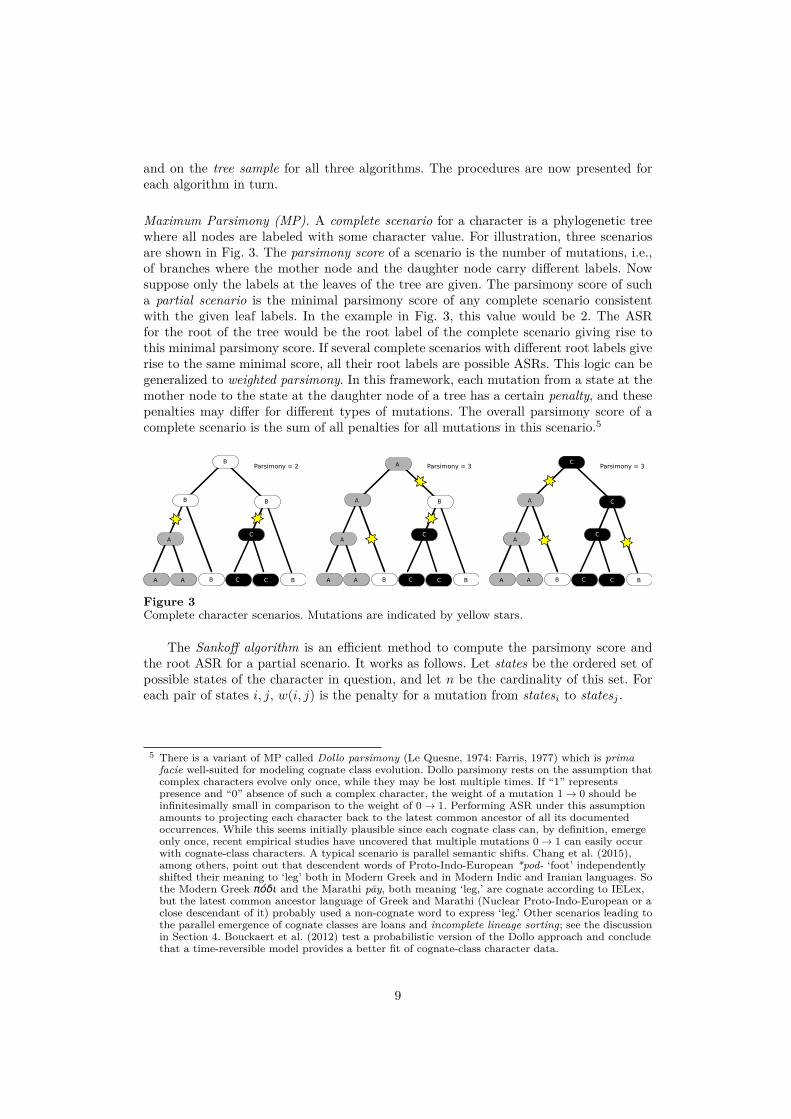
α and β are the equilibrium probabilities of states 1 and 0 respectively, and λ is themutation rate. If t is large in comparison to the minimal time step (such as the time spanof a single generation), we can consider t to be a continuous variable and the entire processa continuous time Markov process. This is illustrated in Fig. 5 for α = 0.2, β = 0.8, andλ = 1. If a language is in state 0 at time 0, its probability to be in state 1 after time tis indicated by the solid line. This probability continuously increases and converges toα. This is the gross probability to start in state 0 and end in state 1; it includes thepossibility of multiple mutations, as long as the number of mutations is odd. The dottedline shows the probability of ending up in state 1 after time t when a language starts instate 1. This quantity is initally close to 100%, but it also converges towards α over time.In other words, the absence of mutations (or a sequence of mutations that re-establishedthe initial state) is predicted to be unlikely over long periods of time. In a completescenario, i.e., a phylogenetic tree with labeled non-terminal nodes, the likelihood of abranch is the probability of ending in the state of the daughter node if one starts in thestate of the mother node after a time interval given by the branch length.

The overall likelihood of a complete scenario is the product of all branch likelihoods,multiplied with the equilibrium probability of its root state. The likelihood of a partialscenario, where only the states of the leaves are known, is the sum of the likelihoods ofall complete scenarios consistent with it. It can efficiently be computed in a way akin tothe Sankoff algorithm. (L(x) is the likelihood vector of node x, and πi is the equilibriumprobability of state i.)

• Initialization. Each leaf l of the tree is initialized with a vector L(l) oflength n, with L(l)i = 1 if l’s label is statesi, and 0 else. (If l ispolymorphic, all labels occuring at t have the same likelihood, and theselikelihoods sum up to 1.)

8 We assume that the rows and columns of P (t) are indexed with 0, 1.

12

0.00

0.25

0.50

0.75

1.00

0.0 2.5 5.0 7.5 10.0t

P(st=1|s0=1)

P(st=1|s0=0)

Figure 5Gain and loss probabilities under a continuous-time Markov process.

• Recursion. Loop through the non-leaf nodes of the tree bottom-up, i.e.,visit all daughter nodes before you visit the mother node. Eachnon-terminal node mother with the set daughters as daughter nodes isannotated with a vector L(mother) according to the rule

L(mother)i =∏

d∈daughters

∑1≤j≤n

(P (t)i,jL(d)j), (6)

where t is the length of the branch connecting d to its mother node.

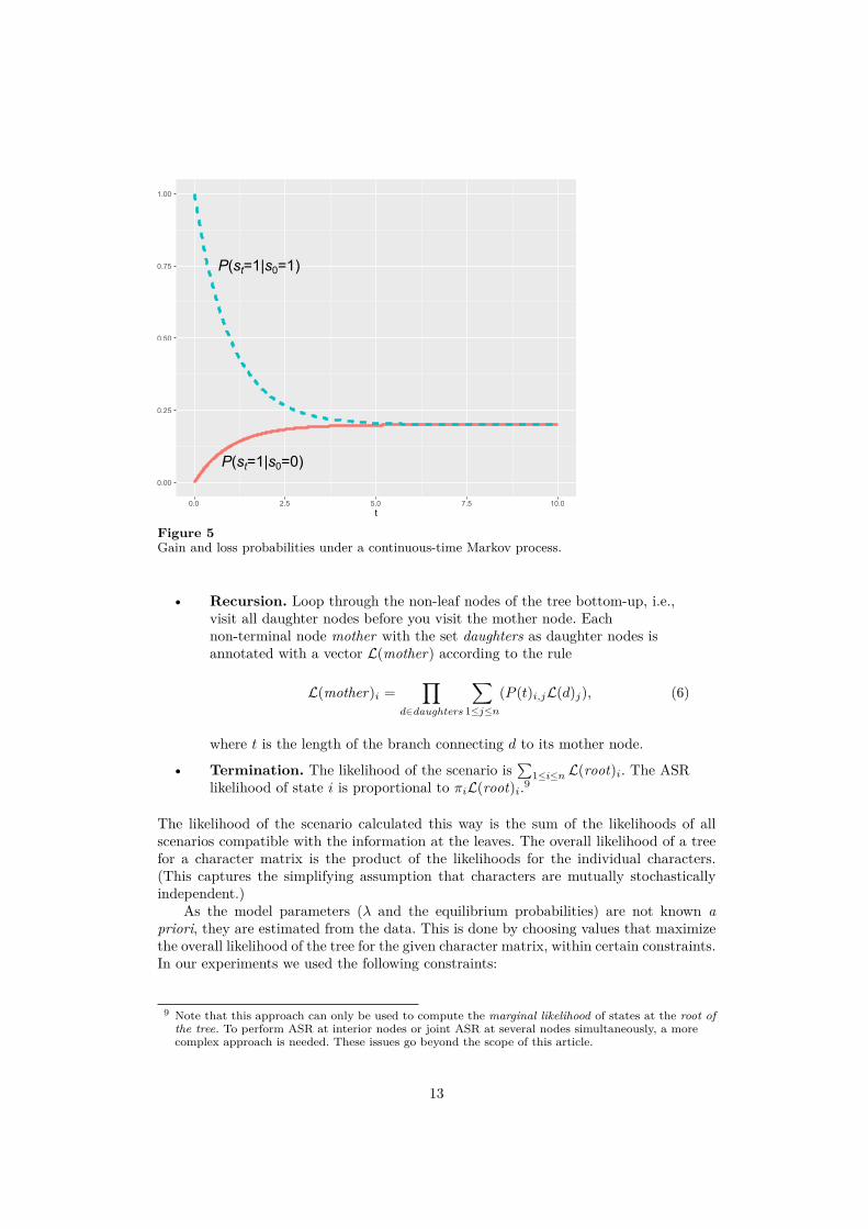
• Termination. The likelihood of the scenario is∑

1≤i≤n L(root)i. The ASRlikelihood of state i is proportional to πiL(root)i.9

The likelihood of the scenario calculated this way is the sum of the likelihoods of allscenarios compatible with the information at the leaves. The overall likelihood of a treefor a character matrix is the product of the likelihoods for the individual characters.(This captures the simplifying assumption that characters are mutually stochasticallyindependent.)

As the model parameters (λ and the equilibrium probabilities) are not known apriori, they are estimated from the data. This is done by choosing values that maximizethe overall likelihood of the tree for the given character matrix, within certain constraints.In our experiments we used the following constraints:

9 Note that this approach can only be used to compute the marginal likelihood of states at the root ofthe tree. To perform ASR at interior nodes or joint ASR at several nodes simultaneously, a morecomplex approach is needed. These issues go beyond the scope of this article.

13

• For multistate characters, we assumed a uniform equilibrium distributionfor all characters, and identical rates for all character transitions.

• For binary characters, we assumed equilibrium probabilities to be identicalfor all characters. Those equilibrium probabilities were estimated from thedata as the empirical frequencies. We assumed gamma-distributed rates,i.e., rates were allowed to vary to a certain degree between characters.

Once the model parameters are fixed, the algorithm produces a probability distributionover possible states for each character. The reconstructed states are identified in a similarway as for Sankoff parsimony. First these probabilities are averaged over all trees if morethan one tree is considered. For multistate characters, the state(s) achieving the highestprobability are selected. For binary presence-absence characters, those cognate classesfor a given concept are selected that achieve the highest average probability for state 1.

2.3 EvaluationFor all three datasets considered, the gold standard contains cognate class assignments fora common ancestor language. For the Chinese data, these are documented data for OldChinese. For the other two datasets, these are reconstructed forms of the supposed latestcommon ancestor (LCA), Proto-Indo-European and Proto-Austronesian respectively.The Old Chinese variety is not identical with the latest common ancestor of all Chinesedialects, but predates it by several hundred years. Due to the rather stable character ofthe written languages as opposed to the vernaculars throughout the history of Chinese,it is difficult to assess with certainty which exact words were used to denote certain basicconcepts, and Old Chinese as reflected in classical sources is a compromise solution as itallows us to consider written evidence rather than reconstructed forms (see Section 4 fora more detailed discussion).

For the evaluation, we only consider those concepts for which (a) the LCA dataidentify a cognate class and (b) this cognate class is also present in one or more of thedescendant languages considered in the experiment. The gold standard defines a set ofcognate classes that were present in the LCA language. Let us call this set LCA. EachASR algorithm considered defines a set of cognate classes that are reconstructed for theLCA. We denote this set as ASR. In the following we will deploy evaluation metricsestablished in machine learning to assess how well these two sets coincide:

precision .=

|LCA ∩ ASR||ASR|

(7)

recall .=

|LCA ∩ ASR||LCA|

(8)

F-score .= 2× precision × recall

precision + recall(9)

The precision expresses the proportion of correct reconstructions among all reconstruc-tions. The recall gives the proportion of ancestral cognate classes that are correctlyreconstructed. The F-score is the harmonic mean between precision and recall.

Results for the various ASR algorithms are compared against a frequency baseline.According to the baseline, a cognate class cc for a given concept c is reconstructed ifand only if cc occurs at least as frequently among the languages considered (excluding

14

algorithm characters tree precision recall F-scorefrequency baseline multi - 0.599 0.590 0.594MLN bin single 0.568 0.729 0.638MLN bin sample 0.568 0.729 0.638Sankoff multi single 0.484 0.743 0.586Sankoff multi sample 0.510 0.722 0.598Sankoff bin single 0.596 0.688 0.639Sankoff bin sample 0.651 0.660 0.655ML multi single 0.669 0.660 0.664ML multi sample 0.669 0.660 0.664ML bin single 0.634 0.625 0.629ML bin sample 0.641 0.632 0.636

Table 2Evaluation results for Chinese

the LCA language) as any other cognate class for c. This baseline comes very close tothe current practice in classical historical linguistics, as presented in Starostin (2016),although it is clear that trained linguists practicing onomasiological reconstruction maytake many additional factors into account. For IELex, we also considered a secondbaseline, dubbed the sub-family baseline. A cognate class cc is deemed reconstructed ifand only if it occurs in at least two different sub-families, where sub-families are Albanian,Anatolian, Armenian, Balto-Slavic, Celtic, Germanic, Greek, Indo-Iranian, Italic, andTocharian.

3 Results

The individual results for all datasets and algorithm variants are given in Tables 2, 3and 4. Note that MLN does not offer a multi-state variant, so for MLN, only results forbinary states are reported. The effects of the various design choices — coding charactersas multi-state or binary; using a single reference tree or a sample of trees — as well as thedifferences between the three ASR algorithms considered here are summarized in Fig. 6.The bars represent the average difference in F-score to the frequency baseline, averagedover all instances of the corresponding category across datasets.

It is evident that there are major differences in the performance of the threealgorithms considered. While the F-score for MLN-ASR remains, on average, below thebaseline, Sankoff-ASR and ML-ASR clearly outperform the baseline. Furthermore, ML-ASR clearly outperforms Sankoff-ASR. Given that both MLN-ASR and Sankoff-ASR dealwith Maximum Parsimony, the rather poor performance of the MLN approach shows thatthe basic vocabulary size criterion may not be the best criterion for penalty selection inparsimony approaches. It may also be related to further individual choices introduced inthe MLN algorithm or our version of Sankoff parsimony. Given that the MLN approachwas not primarily created for the purpose of ancestral state reconstruction, our findings donot necessarily invalidate the approach per se, yet they show that it might be worthwhileto further improve on its application to ancestral state reconstruction.

The impact of the other choices is less pronounced. Binary character coding providesslightly better results on average than multistate character coding, but the effect is minor.

15

algorithm characters tree precision recall F-scorefrequency baseline multi - 0.607 0.497 0.547sub-family baseline bin - 0.402 0.885 0.553MLN bin single 0.781 0.303 0.437MLN bin sample 0.781 0.303 0.437Sankoff multi single 0.367 0.739 0.491Sankoff multi sample 0.566 0.594 0.580Sankoff bin single 0.542 0.630 0.583Sankoff bin sample 0.597 0.503 0.546ML multi single 0.741 0.606 0.667ML multi sample 0.763 0.624 0.687ML bin single 0.778 0.636 0.700ML bin sample 0.785 0.642 0.707

Table 3Evaluation results for IELex

algorithm characters tree precision recall F-scorefrequency baseline multi - 0.618 0.618 0.618MLN bin single 0.843 0.412 0.553MLN bin sample 0.882 0.394 0.545Sankoff multi single 0.688 0.849 0.760Sankoff multi sample 0.726 0.816 0.768Sankoff bin single 0.723 0.771 0.746Sankoff bin sample 0.757 0.749 0.753ML multi single 0.788 0.788 0.788ML multi sample 0.788 0.788 0.788ML bin single 0.776 0.776 0.776ML bin sample 0.771 0.771 0.771

Table 4Evaluation results for ABVD

Likewise, capturing information about phylogenetic uncertainty by using a sample of treesleads, on average, to a slight increase in F-scores, but this effect is rather small as well.

To understand why ML is superior to the two parsimony-based algorithms testedhere, it is important to consider the conceptual differences between parsimony-based andlikelihood-based ASR. Parsimony-based approaches operate on the tree topology only,disregarding branch lengths. Furthermore, the numerical parameters being used, i.e. themutation penalties, are fixed by the researcher based on intuition and heuristics. ML,in contrast, uses branch length information, and it is based on an explicit probabilisticmodel of character evolution.

This point is illustrated in Fig. 7, which schematically displays ASR for the concepteat for the Chinese dialect data. The left panel visualizes Sankoff ASR and the rightpanel shows Maximum-Likelihood ASR. The guide tree identifies two sub-clades, shownas the upper and lower daughter of the root node. The dialects in the upper part of thetree represent the large group of Northern and Central dialects, including the dialect

16

-0.05

0.00

0.05

0.10

aver

age

diffe

renc

e to

freq

uenc

y ba

selin

e

MLMLN Sankoff

algorithms

-0.05

0.00

0.05

0.10

binarymulti

character types

-0.05

0.00

0.05

0.10

single

tree types

sample

Figure 6Average differences in F-score to frequency baseline

of Beijing, which comes close to standard Mandarin Chinese. The dialects in the lowerpart of the tree represent the diverse Southern group, including the archaic Mǐn 闽dialects spoken at the South-Eastern coast as well as Hakka and Yuè 粤 (also referredto as Cantonese), the prevalent variety spoken in Hong Kong. All Southern dialectsuse the same cognate class (eat.Shi.1327, Mandarin Chinese shí 食, nowadays onlyreflected in compounds) and all Northern and Central dialects use a different cognateclass (eat.Chi.243, Mandarin Chinese chī 吃, regular word for ‘eat’ in most Northernvarieties). Not surprisingly, both algorithms reconstruct eat.Shi.1327 for the ancestorof the Southern dialects and eat.Chi.243 for the ancestor of the Northern and Centraldialects. Sankoff ASR only uses the tree topology to reconstruct the root state. Since thesituation is entirely symmetric regarding the two daughters of the root, the two cognateclasses are tied with exactly the same parsimony score at the root. Maximum-LikelihoodASR, on the other hand, takes branch lengths into account. Since the latest commonancestor of the Southern dialects is closer to the root than the latest common ancestor ofthe Northern and Central dialects, the likelihood of a mutation along the lower branchdescending from the root is smaller than along the upper branch. Therefore the lowerbranch has more weight when assigning probabilities to the root state. Consequently,eat.Shi.1327 comes out as the most likely state at the root – which is in accordancewith the gold standard. Our findings indicate that the more fine-grained, parameter-rich Maximum-Likelihood approach is generally superior to the simpler parsimony-basedapproaches.

The parameters of the Maximum-Likelihood model, as well as the branch lengths,are estimated from the data. Our findings underscore the advantages of an empirical,stochastic and data-driven approach to quantitative historical linguistics as compared tomore heuristic and methods with few parameters.

4 Linguistic evaluation of the results

The evaluation of the results against a gold standard can help us to understand thegeneral performance of a given algorithm. Only a careful linguistic evaluation, however,helps us to understand the specific difficulties and obstacles that the algorithms haveto face when being used to analyze linguistic data. We therefore carried out detailedlinguistic evaluations of the results proposed for IELex and BCD: we compared theresults of the best methods for each of the datasets (Binary ML Sample for IELex, and

17

ML

Guangzhou

Suzhou

Meixian

Nanchang

Fuzhou

Ningxia

Lianchang

Ningbo

Yingshan

Chengdu

Zhanping

Shanghai

Shanghai B

Xiamen

Anyi

Beijing

Wenzhou

Taibei

Wuhan

Taiyuan

Yuci

Changsha

Shuangfengeat.Shi.1327eat.Chi.243

Sankoff

Guangzhou

Suzhou

Meixian

Nanchang

Fuzhou

Ningxia

Lianchang

Ningbo

Yingshan

Chengdu

Zhanping

Shanghai

Shanghai B

Xiamen

Anyi

Beijing

Wenzhou

Taibei

Wuhan

Taiyuan

Yuci

Changsha

Shuangfeng

Figure 7Maximum-Likelihood ASR and Sankoff Parsimony ASR for the concept eat for Chinese dialectdata

Multi ML for BCD) with the respective gold standards, searching for potential reasons forthe differences between automatic method and gold standard. The results are providedin Appendix B. In each of the two evaluations, we compared those forms which werereconstructed back to the root in the gold standard but missed by the algorithm, andthose forms proposed by the algorithm but not by the gold standard. By consultingadditional literature and databases, we could first determine whether the error was dueto the algorithm or due to a problem in the gold standard. In a next step, we triedto identify the most common sources of errors, which we assigned to different errorclasses. Due to the differences in the histories and the time depths, the error classeswe identified differ slightly, and while a rather common error in IELex consisted inerroneous cognate judgments in the gold standard,10 we find many problematic meaningsthat are rarely expressed overtly in Chinese dialects in BCD.11 Apart from errors whichwere hard to classify and thus not assigned to any error class, problems resulting fromthe misinterpretation of branch-specific cognate sets as well as problems resulting fromparallel semantic shift (homoplasy) were among the most frequent problems in bothdatasets.

Fig. 8 gives detailed charts of the error analyses for missed and erroneously proposeditems in the two datasets. The data is listed in such a way that mismatches betweengold standard and algorithms can be distinguished. When inspecting the findings forIELex, we can thus see that the majority of the 59 cognates missed by the algorithmcan be attributed to cognate sets that are only reflected in one branch in the Indo-European languages and therefore do not qualify as good candidates to be reconstructedback to the proto-language. As an example, consider the form *pneu̯- (cognate classbreathe:P), which is listed as onomasiological reconstruction for the concept ‘to breathe’

10 See Appendix B1 for details11 Examples include meanings for ‘if’, ‘because’, etc., which may be expressed but may as well be

omitted in normal speech, see Appendix B2 for details.

18

?branch*

cognate*homoplasy* morphology*

sem. shift*

18.6%44.1%

6.8%6.8%

3.4%

20.3%

IELex Missed

?

20.7%?*48.3%

cognate

3.4%

cognate*

13.8%homoplasy

13.8%

IELex Proposed

?

?*

branch

compounding

diffusionmeaning

meaning*2.0%

12.2%

32.7%

44.9%

2.0%4.1%2.0%

BCD Missed

?2.1%

?*

10.6%

branch

12.8%

compounding

36.2%

compounding*

2.1%

diffusion

4.3%

homoplasy

21.3% homoplasy*

2.1% meaning6.4%

meaning*2.1%

BCD Proposed

Figure 8Detailed error analysis of the algorithmic performance on IELex and BCD. If a certain errorclass is followed by an asterisk, this means that we attribute the error to the gold standardrather than to the algorithm. For a detailed discussion of the different error classes mentionedin this context, please see the detailed analysis in the supplementary material.

in the gold standard. As it only occurs in Ancient Greek and has no reflexes in anyother language family, this root is highly problematic, as is also confirmed by theLexicon of Indo-European Verbs, where the root is flagged as questionable (Rix et al.,2001:489). Second, the error statistics for Indo-European contain cognate sets whoseonomasiological reconstruction is not confirmed by plausible semantic reconstructions inthe gold standard. As an example for this error class, consider the form *dhōg̑h-e/os-(cognate class day:B) proposed for the meaning slot ‘day.’ While Kroonen (2013:86f)confirms the reconstruction of the root, as it occurs in Proto-Germanic and Indo-Iranian,the meaning ‘day’ is by no means clear, as the PIE root *di̯eu̯- ‘heavenly deity, day’ isa more broadly reflected candidate for the ‘day’ in PIE (Meier-Brügger, 2002:187f.).

Of the 29 cognates missed, the majority cannot be readily classified, as these comprisecases where a reconstruction back to the proto-language in the given meaning slot seemsto be highly plausible. Thus, the form *kr̥-m-i- (cognate class worm:A) is not listed inthe gold standard, but proposed by the Binary ML approach. The root is reflected inboth Indo-Iranian and in Slavic (Derksen, 2008:93f) and generally considered a validIndo-European root with the meaning `worm, insect' (Mallory and Adams, 2006:149).Given that `worm' and `insect' are frequently expressed by one polysemous concept

19

in the languages of the world (see the CLICS database of cross-linguistic polysemies,List et al., 2014a), we see no reason why the form is not listed in the gold standard.Second in frequency of the items proposed by the algorithm are cases of clear homoplasythat were interpreted as inheritance by the ML approach. As an example, consider theform *serp- (cognate class snake:E), which the algorithm proposes as a candidate forthe meaning `snake.' While the cognate set contains the Latin word serpens, as wellas reflexes in Indo-Iranian and Albanian, it may seem like a good candidate. Accordingto Vaan (2008:558), however, the verbal root originally meant `to crawl,' which wouldmotivate the parallel denotation in Latin and Albanian. Instead of assuming that thenoun already denoted `snake' in PIE times, it is therefore much more likely that we aredealing with independent semantic shift.

Turning to our linguistic evaluation of the results on the Chinese data, we also findbranch-specific words as one of the major reasons for the 49 forms which were proposedin the gold standard but not recognized by the best algorithm (Multi ML). However, herewe cannot attribute these to questionable decisions in the gold standard, but rather to thefact that many Old Chinese words are often reflected only in some of the varieties in thesample. As an example for a challenging case, consider the form口 kǒu `mouth' (cognateclass mouth-Kou-222, # 31). The regular word for `mouth' in most dialects today is 嘴zuǐ, but the Mǐn dialects, the most archaic group and the first to branch off the Siniticfamily, have 喙 huì as an innovation, which originally meant `beak, snout'. While kǒusurvives in many dialects and also in Mandarin Chinese in restricted usage (compare住口zhùkǒu `close' + `mouth' = `shut up') or as part of compounds (口水 kǒushuǐ `mouth'+ `water' = `saliva'), it is only in the Yuè dialect Guǎngzhōu that it appears with theoriginal meaning in the BCD. Whether kǒu, however, is a true retention in Guǎngzhōu isquite difficult to say, and comparing the data in the BCD with the more recent datasetby Liú et al. (2007), we can see that zuǐ, in the latter, is given for Guǎngzhōu insteadof kǒu. The differences in the data are difficult to explain, and we see two possibleways to account for them: (1) If kǒu was the regular term for `mouth' in Guǎngzhōuin the data by Wang (2004), and if this term is not attested in any other dialect, weare dealing with a retention in the Yuè dialects, and with a later diffusion of the termzuǐ across many other dialect areas apart from the Mǐn dialects, which all shifted themeaning of huì. (2) If kǒu is just a variant in Guǎngzhōu as it is in Mandarin Chinese, weare dealing with a methodological problem of basic word translation and should assumethat kǒu is completely lost in its original meaning. In both cases, however, the historyof `mouth' is a typical case of inherited variation in language history. Multiple termswith similar reference potential were already present in the last common ancestor of theChinese dialects. They were later individually resolved, yielding patterns that remindof incomplete lineage sorting in evolutionary biology (see List et al., 2016 for a closerdiscussion of this analogy).

The problem of inherited variation becomes even more evident when we consider thelargest class of errors in both the items missed and the items proposed by the algorithm:the class of errors due to compounding. Compounding is a very productive morphologicalprocess in the Chinese dialects, heavily favored by the shift from a predominantlymonosyllabic to a bisyllabic word structure in the history of Chinese (see Sampson,2015 and replies to the article in the same volume for a more thorough discussion onpotential reasons for this development). This development led to a drastic increase ofbisyllabic words, which is reflected in almost all dialects, affecting all parts of the lexicon.Thus, while the regular words for `sun' and `moon' in Ancient Chinese texts were 日 rìand 月 yuè, the majority of dialects nowadays uses 日頭 rìtóu (lit. `sun-head') and 月光

20

yuèguāng (lit. `moon-shine'). These words have developed further in some dialect areasand yield a complex picture of patterns of lexical expression that are extremely difficultto resolve historically. Given that we find the words even in the most archaic dialects,but not in ancient texts of the late Hàn time and later (around 200 and 300 CE), the timewhen the supposed LCA of the majority of the Chinese dialects was spoken, it is quitedifficult to explain the data in a straightforward way. We could either propose that theLCA of Chinese dialects already had created or was in the stage of creating these ancientcompound words, and that written evidence was too conservative to reflect it; or we couldpropose that the words were created later and then diffused across the Chinese dialects.Both explanations seem plausible, as we know that spoken and written language oftendiffered quite drastically in the history of Chinese. Comparing modern Chinese dialectdata, as provided by Liú et al. (2007), with dialect surveys of the late 1950s, as given inBěijīng Dàxué (1964), we can observe how quickly Mandarin Chinese words have beendiffusing recently: while we find only rìtóu12 as a form for `sun' in Guǎngzhōu, Liú etal. only list the Mandarin form 太陽 tàiyáng, and Hóu (2004), presenting data collectedin the 1990s, lists both variants. We can see from these examples that the complexinteraction between morphological processes like compounding and intimate languagecontact confronts us with challenging problems and may explain why the automaticmethods perform worst on Chinese, despite the shallow time depths of the languagefamily.

5 Conclusion

What can we learn from these experiments? One important point is surely the striking su-periority of Maximum Likelihood, outperforming both parsimony approaches. MaximumLikelihood is not only more flexible, as parameters are estimated from the data, but insome sense, it is also more realistic, as we have seen in the reconstruction of the scenariofor `eat' (see Fig. 7) in the Chinese dataset, where the branch lengths, which contributeto the results of ML analyses, allow the algorithm to find the right answer. Anotherimportant point is the weakness of all automatic approaches and what we can learn fromthe detailed linguistic evaluation. Here, we can see that further research is needed toaddress those aspects of lexical change which are poorly handled by the algorithms. Theseissues include first and foremost the problem of independent semantic shift, but also theeffects of morphological change, especially in the Chinese data. List (2016) uses weightedparsimony with polarized (directional) transition penalties for multi-state characters forancestral state reconstruction of Chinese nouns and reports an increased performancecompared to unweighted parsimony. However, since morphological change and lexicalreplacement are clearly two distinct processes, we think it is more promising to workon the development of stochastic models, which are capable of handling two or moredistinct processes and may estimate transition tendencies from the data. Another majorproblem that needs to be addressed in future approaches is the impact of language contacton lexical change processes, as well as the possibility of language-internal variation,which may obscur tree-like divergence even if the data evolved in a perfectly tree-likemanner. These instances of incomplete lineage sorting (List et al., 2016) became quiteevident in our qualitative analysis of the Chinese and Indo-European data. Given theirpervasiveness, it is likely that they also have a major impact on classical phylogeneticstudies, which only try to infer phylogenies from the data. As a last point, we should

12 In the Yuè dialects, this form has been reinterpreted as `hot-head' 熱頭 rètóu instead of `sun-head.'

21

mention the need for increasing the quality of our test data in historical linguistics. Giventhe multiple questionable reconstructions we found in the test sets during our qualitativeevaluation, we think it might be fruitful, both in classical and computational historicallinguistics, to intensify the efforts towards semantic and onomasiological reconstruction.

Appendices

The appendices contain a list of all age constraints for Indo-European that were usedin our phylogenetic reconstruction study (Appendix A) as well as a detailed, qualitativeanalysis of all differences between the automatic and the gold standard assessmentsin IElex (Appendix B1) and BCD (Appendix B2). They are submitted as part of oursupplementary material.

Supplementary Material

All data used for this study, along with the code that we used and the results we produced,are available at +++zenodo+++.

If readers find error in the code or want to suggest improvements, they are cordiallyinvited to file an issue via our GitHub repository at +++github+++.

The appendices A and B are submitted along with our supplementary material atGitHub and Zenodo.

Acknowledgments

This research was supported by the ERC Advanced Grant 324246 EVOLAEMP (GJ),the DFG-KFG 2237 Words, Bones, Genes, Tools (GJ), the DFG research fellowshipgrant 261553824 (JML) and the ERC Starting Grant 715618 CALC (JML). We thankour anonymous reviewers for helpful comments on earlier versions of this article, as wellas all the colleagues who made their data and code publicly available.

References

Atkinson, Quentin D. and Russell D. Gray. 2006. How old is the Indo-European languagefamily? Illumination or more moths to the flame? In Peter Forster and Colin Renfrew(eds.) Phylogenetic methods and the prehistory of languages, 91--109. Cambridge andOxford and Oakville: McDonald Institute for Archaeological Research.

Ben Hamed, Mahe and Feng Wang. 2006. Stuck in the forest: Trees, networks andChinese dialects. Diachronica 23: 29--60.

Bouchard-Côté, Alexandre, David Hall, Thomas L. Griffiths, and Dan Klein. 2013.Automated reconstruction of ancient languages using probabilistic models of soundchange. Proceedings of the National Academy of Sciences of the United States ofAmerica 110(11): 4224–4229.

Bouckaert, Remco, Joseph Heled, Denise Kühnert, Tim Vaughan, Chieh-Hsi Wu, DongXie, Marc A. Suchard, Andrew Rambaut, and Alexei J. Drummond. 2014. BEAST 2:A software platform for Bayesian evolutionary analysis. PLoS Computational Biology10(4): e1003,537. doi:10.1371/journal.pcbi.1003537. URL http://beast2.org.

Bouckaert, Remco, Philippe Lemey, Michael Dunn, Simon J. Greenhill, Alexander V.Alekseyenko, Alexei J. Drummond, Russell D. Gray, Marc A. Suchard, and Quentin D.Atkinson. 2012. Mapping the origins and expansion of the Indo-European languagefamily. Science 337(6097): 957--960.

22

Bowern, Claire and Quentin D. Atkinson. 2012. Computational phylogenetics of theinternal structure of Pama-Nyungan. Language 88: 817--845.

Bussmann, Hadumod (ed.) . 1996. Routledge dictionary of language and linguistics.London and New York: Routledge.

Běijīng Dàxué 北京大学. 1964. Hànyǔ fāngyán cíhuì 汉语方言词汇 [Chinese dialectvocabularies]. Běijīng 北京: Wénzì Gǎigé.

Campbell, George L. and Gareth King. 2013. Compendium of the World's Languages,vol. 1. London and New York: Routledge.

Chang, Will, Chundra Cathcart, David Hall, and Andrew Garret. 2015. Ancestry-constrained phylogenetic analysis support the Indo-European steppe hypothesis. Lan-guage 91(1): 194--244.

Dagan, Tal, Yael Artzy-Randrup, and William Martin. 2008. Modular networks andcumulative impact of lateral transfer in prokaryote genome evolution. Proceedingsof the National Academy of Sciences of the United States of America 105(29):10,039--10,044.

Derksen, Rick. 2008. Etymological dictionary of the Slavic inherited lexicon. Leiden andBoston: Brill.

Dunn, Michael. 2012. Indo-European lexical cognacy database (IELex). Nijmegen: MaxPlanck Institute for Psycholinguistics. URL http://ielex.mpi.nl/.

Edwards, Anthony W. F. and Luigi Luca Cavalli-Sforza. 1964. Reconstruction ofevolutionary trees. In V. H. Heywood and J. McNeill (eds.) Phenetic and phylogeneticclassification, 67--76. London: Systematics Association Publisher.

Encyclopaedia Britannica, Inc. 2010. Encyclopaedia Britannica. Edinburgh: Encyclopae-dia Britannica, Inc. URL https://www.britannica.com.

Ewans, Warren and Gregory Grant. 2005. Statistical methods in bioinformatics: AnIntroduction. New York: Springer.

Farris, James S. 1977. Phylogenetic analysis under Dollo's law. Systematic Biology 26(1):77--88.

Fitch, Walter M. 1971. Toward defining the course of evolution: minimum change for aspecific tree topology. Systematic Zoology 20(4): 406--416.

Geisler, Hans and Johann-Mattis List. 2010. Beautiful trees on unstable ground. Notes onthe data problem in lexicostatistics. In Heinrich Hettrich (ed.) Die Ausbreitung des In-dogermanischen. Thesen aus Sprachwissenschaft, Archäologie und Genetik [The spreadof Indo-European. Theses from linguistics, archaeology, and genetics]. Wiesbaden:Reichert. URL https://hal.archives-ouvertes.fr/hal-01298493. Document hasbeen submitted in 2010 and is still waiting for publication.

Gray, Russell D. and Quentin D. Atkinson. 2003. Language-tree divergence times supportthe Anatolian theory of Indo-European origin. Nature 426(6965): 435--439.

Gray, Russell D., Alexei J. Drummond, and S. J. Greenhill. 2009. Language phylogeniesreveal expansion pulses and pauses in pacific settlement. Science 323(5913): 479--483.

Greenhill, Simon J., Robert Blust, and Russell D. Gray. 2008. The Austronesian BasicVocabulary Database: From bioinformatics to lexomics. Evolutionary Bioinformatics4: 271--283. URL http://language.psy.auckland.ac.nz/austronesian/.

Hammarström, Harald, Robert Forkel, Martin Haspelmath, and Sebastian Bank. 2015.Glottolog. Leipzig: Max Planck Institute for Evolutionary Anthropology. URL http://glottolog.org.

Haynie, Hanna J. and Claire Bowern. 2016. Phylogenetic approach to the evolution ofcolor term systems. Proceedings of the National Academy of Sciences of the UnitedStates of America 113(48): 13,666--13,671.

23

Holm, Hans J. 2007. The new arboretum of Indo-European ``trees''. Journal ofQuantitative Linguistics 14(2-3): 167--214.

Hóu, Jīngī (ed.) . 2004. Xiàndài Hànyǔ fāngyán yīnkù 现代汉语方言音库 [Phonologicaldatabase of Chinese dialects]. Shànghǎi 上海: Shànghǎi Jiàoyù 上海教育.

Hruschka, Daniel J., Simon Branford, Eric D. Smith, Jon Wilkins, Andrew Meade, MarkPagel, and Tanmoy Bhattacharya. 2015. Detecting regular sound changes in linguisticsas events of concerted evolution. Curr. Biol. 25(1): 1--9.

Huson, Daniel H. 1998. Splitstree: analyzing and visualizing evolutionary data. Bioin-formatics 14(1): 68--73.

Jordan, Fiona M., Russell D. Gray, Simon J. Greenhill, and Ruth Mace. 2009. Matrilocalresidence is ancestral in Austronesian societies. Proceedings of the Royal Society B276: 1957–--1964.

Jäger, Gerhard. 2015. Support for linguistic macrofamilies from weighted alignment.Proceedings of the National Academy of Sciences of the United States of America112(41): 12,752–12,757.

Kassian, Alexei, Mikhail Zhivlov, and George S. Starostin. 2015. Proto-Indo-European-Uralic comparison from the probabilistic point of view. The Journal of Indo-EuropeanStudies 43(3-4): 301--347.

Kitchen, Andrew, Christopher Ehret, Shiferaw Assefa, and Connie J. Mulligan. 2009.Bayesian phylogenetic analysis of Semitic languages identifies an Early Bronze Ageorigin of Semitic in the Near East. Proc. Biol. Sci. 276(1668): 2703--2710.

Kroonen, Guus. 2013. Etymological dictionary of Proto-Germanic. Leiden and Boston:Brill.

Le Quesne, Walter J. 1974. The uniquely evolved character concept and its cladisticapplication. Systematic Biology 23(4): 513--517.

Lee, Sean and Toshikazu Hasegawa. 2013. Evolution of the Ainu language in space andtime. PLoS ONE 8(4): e62,243.

Lepage, Thomas, David Bryant, Hervé Philippe, and Nicolas Lartillot. 2007. A generalcomparison of relaxed molecular clock models. Molecular Biology and Evolution 24(12):2669--2680.

List, Johann-Mattis. 2015. Network perspectives on Chinese dialect history. Bulletin ofChinese Linguistics 8: 42--67.

---------. 2016. Beyond cognacy: Historical relations between words and their implicationfor phylogenetic reconstruction. Journal of Language Evolution 1(2): 119--136. doi:10.1093/jole/lzw006.

List, Johann-Mattis and Robert Forkel. 2016. LingPy. A Python library for historicallinguistics. Jena: Max Planck Institute for the Science of Human History. doi:https://zenodo.org/badge/latestdoi/5137/lingpy/lingpy. URL http://lingpy.org.

List, Johann-Mattis, T. Mayer, A. Terhalle, and M. Urban. 2014a. CLICS: Database ofCross-Linguistic Colexifications. Marburg: Forschungszentrum Deutscher Sprachatlas.URL http://clics.lingpy.org.

List, Johann-Mattis, Shijulal Nelson-Sathi, Hans Geisler, and William Martin. 2014b.Networks of lexical borrowing and lateral gene transfer in language and genomeevolution. Bioessays 36(2): 141--150.

List, Johann-Mattis, Shijulal Nelson-Sathi, William Martin, and Hans Geisler. 2014c.Using phylogenetic networks to model chinese dialect history. Language Dynamicsand Change 4(2): 222–252.

List, Johann-Mattis, Jananan Sylvestre Pathmanathan, Philippe Lopez, and EricBapteste. 2016. Unity and disunity in evolutionary sciences: process-based analogiesopen common research avenues for biology and linguistics. Biology Direct 11(39):

24

1--17.Liú Lìlǐ 刘俐李, Wáng Hóngzhōng 王洪钟, and Bǎi Yíng 柏莹. 2007. Xiàndài Hànyǔ

fāngyán héxīncí, tèzhēng cíjí 现代汉语方言核心词·特征词集 [Collection of basic vo-cabulary words and characteristic dialect words in modern Chinese dialects]. Nánjīng南京: Fènghuáng 凤凰.

Mallory, James P. and Douglas Q. Adams. 2006. The Oxford introduction to Proto-Indo-European and the Proto-Indo-European world. Oxford: Oxford University Press.

Meier-Brügger, Michael. 2002. Indogermanische Sprachwissenschaft [Indo-Europeanlinguistics]. Berlin and New York: de Gruyter, 8th ed.

Mirkin, Boris G., Trevor I. Fenner, Michael Y. Galperin, and Eugene V. Koonin. 2003.Algorithms for computing parsimonious evolutionary scenarios for genome evolution,the last universal common ancestor and dominance of horizontal gene transfer in theevolution of prokaryotes. BMC Evolutionary Biology 3: 2.

Nelson-Sathi, Shijulal, Johann-Mattis List, Hans Geisler, Heiner Fangerau, Russell D.Gray, William Martin, and Tal Dagan. 2011. Networks uncover hidden lexicalborrowing in Indo-European language evolution. Proceedings of the Royal Societyof London B: Biological Sciences 278(1713): 1794--1803.

Pagel, Mark, Quentin D. Atkinson, Andreea S. Calude, and Andrew Meade. 2013.Ultraconserved words point to deep language ancestry across Eurasia. Proceedings ofthe National Academy of Sciences of the United States of America 110(21): 8471--8476.

Pagel, Mark and Andrew Meade. 2014. BayesTraits 2.0. Software distributedby the authors. URL http://www.evolution.rdg.ac.uk/BayesTraitsV3.0.1/BayesTraitsV3.0.1.html.

Rix, Helmut, Martin Kümmel, Thomas Zehnder, Reiner Lipp, and Brigitte Schirmer.2001. LIV. Lexikon der Indogermanischen Verben. Die Wurzeln und ihrePrimärstammbildungen [Lexicon of Indo-European Verbs. The roots and their primarystems]. Wiesbaden: Reichert.

Ronquist, Fredrik, Maxim Teslenko, Paul van der Mark, Daniel L Ayres, Aaron Darling,Sebastian Höhna, Bret Larget, Liang Liu, Marc A Suchard, and John P Huelsenbeck.2012. MrBayes 3.2: efficient Bayesian phylogenetic inference and model choice acrossa large model space. Systematic Biology 61(3): 539--542.

Sagart, Laurent. 2011. Classifying Chinese dialects/Sinitic languages on shared innova-tions. Paris: CRLAO. Paper, presented at the Séminaire Sino-Tibétain du CRLAO(2011-03-28). Online available at https://www.academia.edu/19534510.

Saitou, Naruya and Masatoshi Nei. 1987. The neighbor-joining method: A new methodfor reconstructing phylogenetic trees. Molecular Biology and Evolution 4(4): 406--425.

Sampson, Geoffrey. 2015. A Chinese phonological enigma. Journal of Chinese Linguistics43(2): 679--691.

Sankoff, David. 1975. Minimal mutation trees of sequences. SIAM Journal on AppliedMathematics 28(1): 35--42.

Sokal, R. R. and C. D. Michener. 1958. A statistical method for evaluating systematicrelationships. University of Kansas Scientific Bulletin 28: 1409--1438.

Starostin, G. S. 2016. From wordlists to proto-wordlists: reconstruction as `optimalselection'. Faits de langues 47(1): 177--200. doi:10.3726/432492_177.

Swadesh, Morris. 1952. Lexico-statistic dating of prehistoric ethnic contacts. Proceedingsof the American Philosophical Society 96(4): 452--463.

---------. 1955. Towards greater accuracy in lexicostatistic dating. International Journalof American Linguistics 21(2): 121--137.

The LINGUIST List. 2014. Multitree: A digital library of language relationships. Bloom-ington: Indiana University. Department of Linguistics. URL http://multitree.org.

25

Urban, Matthias. 2011. Asymmetries in overt marking and directionality in semanticchange. Journal of Historical Linguistics 1(1): 3--47.

Vaan, Michiel. 2008. Etymological dictionary of Latin and the other Italic languages.Leiden and Boston: Brill.

Wang, Feng. 2004. Bcd: Basic words of chinese dialects.Wessen, Elias. 1968. Die nordischen Sprachen [The Nordic languages]. Berlin: de

Gruyter.Wilkins, David P. 1996. Natural tendencies of semantic change and the search for

cognates. In Mark Durie and Malcom Ross (eds.) The comparative method reviewed.Regularity and irregularity in language change, 264--304. New York: Oxford UniversityPress.

Yang, Ziheng and Bruce Rannala. 1997. Bayesian phylogenetic inference using DNAsequences: a Markov Chain Monte Carlo method. Molecular biology and evolution14(7): 717--724.

Zhou, Kevin and Claire Bowern. 2015. Quantifying uncertainty in the phylogenetics ofAustralian numeral systems. Proceedings of the Royal Society B 282(1815): 20151,278.

26

27