Using Weekly Empirical Probabilities in Currency Analysis ... · Andrew C Pollock, Alex Macaulay,...

Electronic copy available at: http://ssrn.com/abstract=1542597

Using Weekly Empirical Probabilities in Currency Analysis and Forecasting

Andrew C Pollock1,

Alex Macaulay1

Mary E Thomson2

Dilek Önkal3

Abstract The Empirical Probability (EP) technique is proposed as an effective support tool to assist agents operating in a global fusion of financial markets. This technique facilitates the identification and prediction of primary, secondary and tertiary trends in addition to the recognition of trend reversals and the detection of changes in trend momentum. The suggested procedure is illustrated by deriving weekly (five-day) non-overlapping estimated probabilities from daily Euro/USD exchange rate data from 04/01/1999 to 31/12/2004 and applying these probabilities to the analysis and forecasting of exchange rate movements. In addition, trend characteristics of the data are used to develop a trading system that not only provides buy and sell indicators but also supplies directional probabilities associated with the signalled actions. Key Words: Foreign Exchange, Forecasting, Investment Decisions JEL Classification: F31, F47, G11 and G15

Corresponding Author. E-Mail: [email protected], Tel: ++ 44 141 331 3613 Fax: ++ 44 141 331 8445. 1 Unit of Mathematics, Division of Communications, Network and Electronic Engineering, School of Engineering and Computing, Glasgow Caledonian University, Cowcaddens Road, Glasgow, G4 0BA, UK.

2 Division of Psychology, Glasgow Caledonian University, Cowcaddens Road, Glasgow, G4 0BA, UK, E-Mail: [email protected] 3 Faculty of Business Administration, Bilkent University, 06800 Bilkent, Ankara, Turkey, [email protected].

Electronic copy available at: http://ssrn.com/abstract=1542597

Andrew C Pollock, Alex Macaulay, Mary E Thomson, Dilek Önkal – Using Weekly Empirical Probabilities in Currency Analysis and Forecasting – Frontiers in Finance and Economics – Vol. 5 No.2 – October 2008, 26 – 55

1 - Introduction Exchange rates not only exhibit volatility but also display trends that

directly influence the quality of financial decisions involving the international securities and foreign exchange markets. Recognizing changing trend conditions (in particular, the identification of trend reversals and momentum changes) is a basic requirement for successful currency analysis and effective forecasting. Trends tend to mirror the general levels of optimism/pessimism and accompanying uncertainty assessments of financial players, aggregating to form bullish and bearish sentiments for a particular currency. Writing over a century ago, Charles Dow, identified three main types of trend:

(i) Major or primary trends tend to last for more than one year and provide a synthesis of the market sentiment dominating in the longer term;

(ii) Intermediate or secondary trends tend to last from one to several months and reflect short term corrections/reactions of market sentiment;

ii) Minor or tertiary trends tend to last for a maximum of several weeks, and arise to a large extent from recent trading activities.

This concept of multiple trends, with each trend becoming a portion of a larger trend, is a basic premise of technical analysis [Murphy, 1999], an approach which is widely used by analysts in foreign exchange markets [Taylor and Allen, 1992; Cheung and Chinn, 2001].

The importance of identifying various trend conditions has motivated the procedure proposed in current work. In particular, this paper illustrates that weekly empirical probabilities (EPs) provide valuable tools to aid currency analysts in successfully identifying and predicting trend conditions. It is shown that EPs derived from daily movements in the logarithms of the exchange rate over a five-day period can be used to provide effective directional predictions for the relevant forecast horizon. The EP technique used in this paper is based on the assumption that changes in the logarithms of exchange rates follow a Normal distribution with a time-varying mean and standard deviation. The distribution mean reflects the varying degrees of optimism and pessimism as manifested in immediate term drift (tertiary trends) within short-term drifts (secondary trends) which, themselves, are also within longer-term drifts (primary trends). The distribution standard deviation reflects variations in uncertainty assessments of market participants over the time period being considered.

Using a five-day time frame, the proposed technique computes the empirical probabilities and illustrates their role in currency analysis and


forecasting. The procedure is demonstrated via the derivation of weekly (i.e., five-day) EPs for daily Euro/US Dollar (EUR/USD) exchange rates from 04/01/1999 to 31/12/2004. Five-day-ahead EP predictions are then derived from a weighting procedure of component EPs that are specified to identify primary, secondary and tertiary trend conditions. Current work also illustrates how the EP predictions can be used judgementally and/or statistically to aid decisions that involve buy and sell actions. The procedure is then extended to develop a method by which EP predictions can be used as a support core for an effective trading and investment system.

The paper is structured as follows: Section 2 discusses the importance of primary, secondary and tertiary trends to exchange rate behaviour. Section 3 sets out the methodology for deriving EPs. These concepts are then applied to develop a procedure to form one-week-ahead predictions and a trading/investment system. Section 4 applies this procedure to the empirical analyses of the EUR/USD, using daily data from the inception of the Euro until the end of 2004, presenting and evaluating the results from the derived trading/investment system. The discussion and conclusions are given in Section 5.

2 - Exchange rate behaviour and reflections on primary, secondary and tertiary trends


Financial players’ uncertainty, attitudes and judgements of dominant market sentiment play fundamental roles in their prediction of currency movements [Larson and Madura, 2001]. Psychological factors influencing market participants may be viewed as being reflected on the statistical distribution of exchange rate movements with the mean summarizing collective optimism/pessimism, and the standard deviation synopsizing the aggregate uncertainties. Overall, trends in exchange rates echo the uncertainty, perceptions and subsequent expectations of participating agents, and thus identifying and predicting trends remain focal points of financial research. The ideas surrounding primary, secondary and tertiary trends are originally introduced by Charles Dow. He presents his ideas, which relate to his work with Edward Jones (i.e., via the Dow Jones and Company), in a series of editorials in the Wall Street Journal, at the turn of the last century [reprinted in Nelson, 1903]. Even though Dow’s views on trends are specifically focused on the US Industrial and Railway sectors, these concepts are extremely relevant to today’s foreign exchange markets.

Specifically, Dow proposes that the market has three main trends: primary, secondary and tertiary. In predicting exchange rate movements over the immediate, short and long terms, an awareness of the existence of often contradictory trend patterns is critical. Dow made an analogy of the differing types of trends with tides, waves and ripples of the sea. Primary trends are viewed as being similar to the tides. Generally lasting for more than one year, primary trends reflect the underlying long term bullish or bearish sentiment against a currency and are, therefore, associated with a relatively stable distribution over time. Primary trends are more likely to continue than to reverse [Murphy, 1999]. The identification of these long term trends is critical and forms the basis for the prediction of exchange rate movements over both the long and short terms.

Secondary trends are compared with the waves. Typically lasting between one and several months, secondary trends are shorter term and basically mirror various corrective actions of the financial players. For example, market participants may feel that short term excessive bullish sentiment regarding a specific currency has been too strong and that the change in the exchange rate over the last months has been excessively large, hence they review their positions. Secondary trends can, therefore, cause the location parameter of the distribution of daily exchange rate movements, implied by the primary trend, to change in relatively short periods, resulting in lower/higher mean changes in the short run, and even a mean reversal. Such


shifts can explain why the mean of the distribution may be relatively stable over short periods of time but appears to change over longer horizons. In addition, the market will also be influenced by periods of stability and instability that are associated with shorter term uncertainty assessments of market participants. Their reactions to such assessments cause variability in the dispersion parameter over relatively short periods of time. In sum, the identification of secondary trends is essential, especially when exchange rate predictions are made for intervals of less than six months.

Tertiary trends are viewed as being like the ripples. Lasting between one and several weeks, tertiary trends are often associated with very short term trading activity and are not usually of direct interest when the forecast horizon exceeds one week. Their very nature can, however, cause substantial daily volatility that can make exchange rate predictions for daily and weekly movements extremely difficult.

Primary, secondary and tertiary trends interact with each other forming cycles, with each cycle being part of a larger cycle. That is, the ripples (tertiary trends) feed into the waves (secondary trends), which in turn flow into the tides (primary trends). It is thus critical to incorporate these three types of trend into the analysis and prediction of exchange rate movements, as they are likely to cause the distribution to exhibit changing means and variances over time.

The presence of multiple trends is consistent with recent financial literature on momentum. A number of studies relating to equity markets imply that there are short run momentum profits but these are reversed in the long run [Jagadeesh and Titman, 2001, Cooper, Gutierrez and Hameed, 2004]. In relation to the currency markets Evans and Lyons (2003), using intraday data, found that over horizons of one day, news announcements affect exchange rates through currency flows. Froot and Ramadorai (2005) established that currency flows from institutional investors, arising from deviations of the exchange rate from its intrinsic value (changes in the real exchange rate), can cause short term momentum impacts (of up to 30 days) in currency returns which are roughly offset by longer term reversal effects. Currency flows can explain transitory excess returns causing short run underreaction and long run overreaction. In long horizons their results lend support to the fundamental view that interest rate differentials are an important factor but currency flows are not. This mechanism could certainly contribute to the presence of secondary and tertiary trend effects in the EUR/USD.

The existence of seasonal factors could be an alternative explanation


of multiple trends. Studies have indicated that daily, monthly, annual and holiday effects can exist in equity indices [Lakonishok and Smidt, 1988] with weekend effects attracting particular attention [Jaffe and Westerfield, 1985; Kamara, 1997]. In currency markets there exists evidence that day-of-the-week effects can cause different distributions or parameters between the five trading weekdays. McFarland, Pettit and Sung (1982) pointed out that the rate of information flow to the market varies, not only with the time of the day, but also with the day of the week and this can have an important impact on exchange rate movements. For instance, Monday’s change can be different from that of other days [Hsieh, 1988]. The vastly increased trading and turnover in the currency markets since 1990, however, has tended to remove seasonal abnormalities in daily mean returns. The weekend period, when the world's foreign exchange markets are closed (i.e., between US Friday market close and the New Zealand Monday market opening, local time), is generally a period when very few economic announcements are made. Even when significant events do occur in this weekend period market participants would have more time to cognitively process this information compared with the rest of the week when the world's markets are open for 24-hours. This is likely to reduce any weekend overreaction to events. Mondays change, therefore, is not likely to be significantly different from other days. Trading day effects are not, therefore, believed to explain currency tertiary trends.

3 - Methodology

To examine the issues set out in Section 2 and to develop a procedure

to properly identify various types of trend, a technique utilising empirical probabilities (EPs) is proposed. This is followed by a portrayal of a trading/investment model based on weekly EPs, with extensions to a trading/investment system involving Euro/USD predictions. Appropriate parameters for the model and the trading/investment system are identified and a method based on the profitability of buy/sell actions is set out to evaluate the system’s performance.

3.1 Deriving empirical directional probabilities

EPs are based on the assumption that the changes in logarithms of

exchange rates can be considered to be approximately Normal with stable means and standard deviations over short horizons. Evidence suggests that this


assumption is appropriate for daily sampling frequencies of the major exchange rates over periods of 30 days or less [Pollock et al, 2002, 2004, 2005]. EPs calculated from daily data over a five day horizon can be obtained using the Normality assumption and then used as indicators of primary, secondary and tertiary trends. The starting point to obtaining weekly EPs is to calculate the first differences in the logarithms of the exchange rate series for a given day over a five trading day period using the current and preceding exchange rate values. Given daily values of an exchange rate series, tX , at day

t, the logarithms (to base 10) of the series, tx , are obtained, i.e. tt Xx 10log .

Then daily first differences are taken, tx (where 1 ttt xxx ). There are strong reasons for using first differences of logarithms on statistical grounds as exchange rate series are not stationary, i.e., their autocovariance functions depend on time. In particular, the variance tends to increase over time and first order serial correlation occurs with a value close to unity. In other words, the logarithms of the series tend to follow what is described by Nelson and Plosser (1982) as a difference-stationary process. Evidence suggests that trends in exchange rate series tend to be associated with first order positive serial correlation of unity. Using first differences simultaneously removes a linear trend and serial correlation of unity.

Drift can be identified by the mean, tm , of the changes in logarithms, over a five day interval (t-4,t), defined in equation (1):

4

05

1

iitt xm (1)

These means can be calculated each day, t, identifying changes in the drift over time.

The volatility of the changes in a financial series can be examined by calculating the standard deviation, ts , of changes in the logarithms of the data over the same interval, as defined in equation (2):

24

0

)(4

1t

iitt mxs

(2)

These standard deviations can also be calculated each day, t, revealing the extent of volatility in exchange rates.

The next stage is the calculation of a t-value that reflects the change in the mean over the five day period scaled by the standard deviation. The ratio of the mean ( tm ) to the standard deviation ( ts ) is multiplied by the square


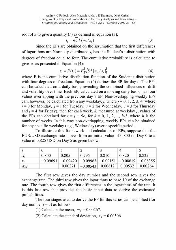
root of 5 to give a quantity (tt) as defined in equation (3):

)/(*5 ttt smt (3)

Since the EPs are obtained on the assumption that the first differences of logarithms are Normally distributed, tt has the Student’s t-distribution with

degrees of freedom equal to four. The cumulative probability is calculated to give te as presented in Equation (4):

tttt smFFe /*5)t( (4)

where F is the cumulative distribution function of the Student t-distribution with four degrees of freedom. Equation (4) defines the EP for day t. The EPs can be calculated on a daily basis, revealing the combined influences of drift and volatility over time. Each EP, calculated on a moving daily basis, has four values overlapping with the previous day’s EP. Non-overlapping weekly EPs can, however, be calculated from any weekday, j, where j = 0, 1, 2, 3, 4 (where j = 0 for Monday, j = 1 for Tuesday, j = 2 for Wednesday, j = 3 for Thursday and j = 4 for Friday), then for each week, k, measured at weekday j, values of the EPs can obtained for t = j + 5k, for k = 0, 1, 2,…, h-1, where h is the number of weeks. In this way non-overlapping, weekly EPs can be obtained for any specific weekday (e.g., Wednesday) over a specific period.

To illustrate this framework and calculation of EPs, suppose that the EUR/USD exchange rate moves from an initial value of 0.800 on Day 0 to a value of 0.825 USD on Day 5 as given below:

t 0 1 2 3 4 5 Xt 0.800 0.805 0.795 0.810 0.820 0.825 xt 0.09691 0.09420 0.09963 0.09151 0.08619 0.08355 Δxt 0.00271 0.00543 0.00812 0.00532 0.00264

The first row gives the day number and the second row gives the exchange rate. The third row gives the logarithms to base 10 of the exchange rate. The fourth row gives the first differences in the logarithms of the rate. It is this last row that provides the basic input data to derive the estimated probabilities.

The four stages used to derive the EP for this series can be applied (for day number t = 5) as follows:

(1) Calculate the mean, 5m = 0.00267.

(2) Calculate the standard deviation, 5s = 0.00506.


(3) Obtain the t value, )00506.0/00267.0(*5t5 = 1.182.

(4) Obtain the cumulative probability, )182.1(5 Fe = 0.849, using

Student’s t-distribution with four degrees of freedom. The EP is 0.849, corresponding to a rise in the exchange rate. In practice, overlapping daily and non-overlapping weekly EPs can be

calculated for any given day over a five day span to give weekly EPs stating at any desired weekday, j and day t. These EPs can then be presented on a graph and used to examine the characteristics of the exchange rate movements and aid in the making of buy and sell predictions. They can act as indicators that reflect the strength of the direction of trend movement and market momentum and can be used to form the basis of a trading/investment system.

EPs have desirable properties that aid the interpretation of exchange rate movements. These are:

i) EP values provide a direct indicator of market momentum in a form constrained by an upper bound of unity and a lower bound of zero. The existence of zero-unity bounds for EPs allows unambiguous interpretations and consistent evaluations of market activity.

ii) Statistically significant movements can be directly identified from the EPs. Values below a lower critical value or above an upper critical value indicate that a significant move in the exchange rate has occurred. For instance, critical values of 0.025 and 0.975 would correspond to rejection, at the 5% level of significance, of the null hypothesis that the true mean change is zero.

iii) EP values provide a measure that is consistent with measures of the profitability related to action decisions. A profit or loss over the period, on which the EPs are calculated, is easily seen. That is, values below 0.5 indicate a loss and values above 0.5 indicate a profit.

iv) Volatility is directly incorporated into the EPs via the inclusion of the standard deviation of changes (in logarithms) in their construction. This is extremely useful as the presence of drift is examined in a form that takes out any influences from changing volatility that can cloud the picture. Hence, secondary trends are easily seen in high and low volatility periods.

EPs are equally applicable to trending and flat trend markets. In flat trend markets, EPs will show values centred around 0.5 but in trending markets the values will be centred above 0.5 (uptrend) or below 0.5 (downtrend). Weekly EPs, however, will tend to show considerable variability due to activity associated with tertiary trends. In the long term, in upward


primary trending markets, the EPs will tend to have the majority of values concentrated above 0.5 and in downward primary trending markets, the EPs will tend to have the majority of values concentrated below 0.5. Over short horizons of three months or less, however, the concentration of values will be largely influenced by secondary trends. For weekly EPs these patterns tend to be masked by the considerable volatility. The primary and secondary trend can, however, be more clearly seen by taking a moving average of the weekly EPs. Moving averages of EPs have the advantage that they can be used as an indicator of a change in the trend as shown by the EPs reaching a peak or trough in the appropriate trend period. The interpretation of EPs is very dependent on the experience of the analyst using the technique. When using weekly EPs it is generally better to use the EP chart in conjunction with a chart of the logarithms of the actual series to give a more holistic view of the situation.

3.2 Procedure to form predictions of the empirical probabilities

A procedure was developed to provide a prediction of the EP five

trading days (or one week) ahead based on a weighted average of components relating to the primary, secondary and tertiary trends. The prediction, denoted 1ˆ te , made at the end of week t for the EP at the end of week t + 1, is

given in equation (5): 1,331,221,111 ˆˆˆˆ tttt eveveve (5)

where 1,31,21,1 ˆ and ˆ,ˆ ttt eee are components relating to the primary,

secondary and tertiary trends respectively, and 1v , 2v and 3v represent weights

which sum to unity (e.g., 1v = 0.3, 2v = 0.6 and 3v = 0.1). It is, of course,

necessary to ensure that 1ˆ0 1 te which is satisfied with the condition that

1ˆ0 1, tje for j = 1, 2, 3.

Each trend component measure êj,t+1 is based on a moving average of the current and past weekly EPs, a term that picks up the change in the EP over the period jnt to jn , and a correction factor of unity, as defined in

equation (6):

1

01, 1

2

1ˆ

j

j

n

inttit

jtj eee

ne , j = 1, 2, 3 (6)


where nj is the order of the moving average, in number of weeks, used

for the three types of trend. The rationale for this specification can be better understood by writing

equation (6) as:

2222

1ˆ

1

11,

j

ntt

j

n

iit

j

t

jtj n

ee

n

e

n

e

ne j

j

(7)

The term 2/1 jn ensures that 1,ˆ tje has a value between zero and

one. The momentum term 2/ jt ne reflects the movement in the exchange

rate over the current (i.e. the most recent) week. The importance of both these components lessens as the order of the moving average, nj, increases. The

average of the previous momentum terms 2/1

1

j

n

iit ne

j

reflects past

movements in the exchange rate over the period 1 jnt to 1t . The

importance of this component increases as the order, jn , increases and for

large values of jn this term dominates.

The term 2/ jntt neej

reflects the change in the EP over the

period jnt to t and is related to the acceleration or deceleration of exchange

rate movements over the period. The importance of this component decreases the longer the trend component horizon and can be particularly influential for low values of jn (e.g., 2or 1jn ).

To apply the above model specification the next stage is to assign values for the jn , j = 1, 2, 3. For the primary trend component 1n should be

large enough to distinguish the primary trend from the secondary trend, say at least twice the normal length of the secondary trend (equivalent to the length of the secondary cycle) but short enough not to exceed the normal length of the primary trend. In currency markets secondary trends are unlikely to be greater than 30 weeks and primary trends are likely to be longer than one and a half years, hence a value for 1n of 60 might be appropriate. For the


secondary trend component 2n should be large enough to distinguish the

secondary trend from the tertiary trend, say at least twice the normal length of the tertiary trend (equivalent to the length of the tertiary cycle), but short enough not to exceed the normal length of the secondary trend. In currency markets tertiary trends are unlikely to be greater than 3 weeks and secondary trends are likely to be shorter than 6 weeks, hence a value for 2n of 6 might be

appropriate. For the tertiary trend component the choice of value for 3n is

limited by its normal maximum length of 3 weeks and the fact that a minimum of one week is required (with daily data) to obtain the EP. In currency markets a value for 3n of 1 might, therefore, be appropriate.

Taking 3n = 1 in (7) gives:

3/1ˆ 11,3 tttt eeee (8)

Equation (8) implicitly allows more weight to be given to a particular magnitude of weekly change in the EP when the current EP is close to 0.5 than when it is close to either zero or unity. For instance, if the EP is near its maximum (minimum) value of unity (zero), any predicted rise (fall) in the tertiary trend would numerically be small as the potential increase (decrease) would have to be small in magnitude. When, however, the current EP is near to 0.5, little trend is indicated in the actual exchange rate series and changes in the EP, in either direction, are likely to have an important impact in predicting its value the following week. Equation (8) also allows for a high likelihood of trend reversal or at least for the EP to regress towards the value of 0.5. Given the limited length of tertiary trends it would not be reasonable to generate predictions that give a high 1,3ˆ te over more than two weeks. For instance, if

2te = 0.1 and 1te = 0.9, then the value te ,3ˆ = 0.9 obtained from equation (8)

could be considered reasonable. If, in fact, te = 0.9, the value of ê3,t+1 = 0.63

obtained from equation (8) would signal the trend weakening or reversing. The above would also be relevant, to a lesser extent, for the secondary component but the increased importance of the previous momentum term considerably reduces this effect and for the primary component the effect is virtually non-existent.

The primary, secondary and tertiary components are, of course, not independent of each other. Each secondary trend is made up of a number of tertiary trends and each primary trend is made up of a number of secondary trends. In the choice of weights it is important to take account of this. Given


that the interest is in a five day ahead prediction, the secondary component weight is likely to be the most important. Hence, a value of 0.6 or above (i.e., 6.02 v ) would be appropriate. The primary trend component weight

would, of course, be lower but still reasonably high whenever a clear upward or downward primary trend is present. Hence, a value of 0.4 or less (i.e., 4.01 v ) might be considered appropriate. The tertiary component would

be expected to have a lower weight than the secondary component although it could be important in volatile conditions when immediate term exchange rate movements dominate. Hence, a value of 0.4 or less (i.e., 4.03 v ) might

generally be appropriate. In practice, the formation of the one week ahead EP predictions could

be made by setting the weights, either judgmentally or statistically, in response to market conditions and changing the weighting when market conditions are perceived to have changed. Furthermore, the length of the periods used could also be changed to account for the variable periods of secondary and primary trends. The resulting predictions would then provide a basis for buy and sell actions involving the Euro. The EP predictions themselves, of course, not only provide a directional indicator of the exchange rate movement but also a measure of confidence, a probability, on which action decisions can be based. Furthermore, in addition to profitability performance evaluation from actions decisions, the predicted EPs can be examined over a range of values and directly compared with the ex-post weekly EPs to evaluate predictive performance.

The procedure set out above can be further developed to provide a basis for a trading/investment system that could be used to generate buy and sell actions. Specifically, the procedure can be applied to examine the impact of different weights, 1v , 2v and 3v , on the average weekly percentage profit

for each choice which can then be compared with that of the ‘always hold EUR’ strategy. Setting up a trading/investment system is discussed in the next sub-section.

3.3 Setting up a trading / investment model

In developing a procedure to give weekly action decisions the

predictions obtained from sub-section 3.2 are used. The trading/investment system is based on the EP prediction for week

t + 1 and the difference between that prediction and the EP prediction for


week t. Specifically, in terms of the EUR/USD exchange rate: i) an action decision to hold EUR would occur if 5.0ˆ 1te and

to hold USD if 5.0ˆ 1te , where α is an arbitrary positive constant;

ii) for values 5.0ˆ5.0 1te , the decision would be to

change holding from EUR to USD if both 5.0ˆ5.0 1 te and

tt ee ˆˆ 1 and to change from USD to EUR if both 5.0ˆ5.0 1te and

tt ee ˆˆ 1 ;

iii) in all other cases, no change to the current holding would take place.

The procedure is used to generate actions to be taken at time t, the effects of which are evaluated at time t + 1. As the predicted EPs essentially reflect a smoothed series, low values of α between 0 and 0.15 would, generally, be appropriate. There are, however, factors to consider in setting the values for α. Low values of α (e.g., 0 or 0.05) would tend to give more buy/sell action changes than higher values. This may not be a problem in a currency trading context but could be undesirable, for instance, where Euro and USD assets were held in equity portfolios. A high number of buy/sell actions would, particularly, be a problem when higher weightings are given to the tertiary component (e.g., 3v = 0.3 or 0.4) as the resulting EP series would

show more variation than when a lower weighting is used. It is, therefore, appropriate to consider the tertiary weighting, 3v , when setting . For instance,

when 3v has values of 0 or 0.1, α values of 0 or 0.05 could be appropriate,

when 3v has values of 0.2 or 0.3, α values of 0.05 or 0.1 could be appropriate

and when 3v has a value of 0.4, α values of 0.1 or 0.15 could be appropriate.

Consider a US investor who can hold all his assets in either EUR or USD. A buy action results in holding all assets in EURs and a sell action results in holding all assets in USDs. It is assumed, for convenience, that the interest rate on EUR and USD assets is identical and that there are no transaction costs. Profitability performance is examined on a week-to-week basis: given an investor with an initial amount 0A on a specific day of week 0,

the value kA of this investment on the same day of the week in a future week,

k, is ascertained from Equation (9):


k

i i

iiik X

XXdAA

0 1

10 1 (9)

where iX is the value of the ER on the specific day of week i. The 0/1

indicator variable, id , corresponds to the action decision, viz., id = 0 implies

hold USDs and id = 1 implies hold EURs.

4 - The Analysis of the EUR/USD

4.1 The data

The weekly EPs were computed from daily data for the EUR/USD

(and USD/EUR) for the period beginning at the first day of trading of the Euro, Monday 04/01/99, to Friday 31/12/04. This currency pair is an appropriate choice as turnover in the EUR/USD accounted for 28% of total global foreign exchange market turnover in 2004 [Bank for International Settlements, 2005]. The daily data were obtained from Norgate Investor Services using their Premium End-of-Day Forex service data set. The closing price was taken from quotations prevailing at 5.00 pm, New York time. These data are multi-sourced arising from combining quotations from a range of contributors.

There were weekdays when data were not available that were associated with holiday periods. These amounted to 15 days with dates as follows: 02/04/99; 03/01/00; 21/04/00; 25/12/00; 01/01/01; 13/04/01; 25/12/01; 01/01/02; 2/903/02; 25/12/02; 01/01/03; 18/04/03; 25/12/03; 01/01/04; 09/04/04. A graph of the actual data over the period is presented in Diagram 1. To allow the lengths of trends to be more easily interpreted the days are numbered on the horizontal axis from 0 (04/01/99) to 1564 (31/12/04) and included weekdays when data were not available (identified above).

Diagram 1 shows a clear downward primary trend in the first third of the graph which reversed to give a clear upward primary trend in the second half of the graph. There is also evidence of secondary trends reflected in cycles with variable periods of around 150 days. There is some evidence of higher frequency, variable period cycles with periods around 15 days which can be interpreted as tertiary trends. In addition, there are possibly other minor cycles with periods between the secondary and tertiary cycles.


4.2 The weekly empirical probabilities Logarithms of the daily series were taken and first differences

calculated. The first 5 differences, calculated on the trading days from Tuesday 05/01/99 to Monday 11/01/99 inclusive, were used to obtain the EP for Monday 11/01/99 from equation (4); the remaining EPs were similarly calculated, based on moving 5-day periods. The analysis used the closing values on Wednesday to calculate the weekly EPs. This resulted in 312 weekly EPs which were numbered from 1 to 312 (excluding the first week). On weeks which were affected by weekdays when data were not available, the EPs were calculated using 4 daily changes (rather than 5). The EPs together with the logarithms of the actual values (scaled to lie between zero and one) are presented in Diagram 2. The above procedure was also applied to closing values, in a similar way, for Monday, Tuesday, Thursday and Friday closing rates, although the results are not presented here.

Diagram 2 shows that the weekly EPs exhibit considerable variation mainly due to the tertiary trend effects. Underlying cyclical patterns with variable periods around 30 weeks reflect secondary trend influences. The primary trends are characterised by the majority of the values falling in the bottom half of the graph as in the first third of the graph and upward primary trends have values falling in the upper half of the period as in the last third of the period.

4.3 Examining the normality assumption

In the calculation of EPs set out above, the assumption of Normality is

crucial. The validity of this assumption was examined by using the Anderson Darling (A-D) [Anderson and Darling, 1954] empirical distribution test. The test values and probabilities were obtained using the Minitab statistical software package.

The A-D test is preferred to the Kolmogorov - Smirnov (K-S) as it gives more weight to the tails. In a comparison of the K-S and A-D tests, Seier (2002) showed that for 20 observations, the A-D test was generally more powerful than the K-S test. Other more powerful tests that rely on third and fourth moments are not appropriate for series with a small number of observations as these moments are likely to be unstable [Harvey, 1993].


The evidence suggests that the distribution of changes in the logarithms of daily exchange rates follow a Normal distribution with changing means and variances over time. Over short horizons, however, the distribution can be viewed as approximately following a stable Normal distribution [Pollock et al, 2002, 2004, 2005].

In the calculation of EPs a crucial assumption in applying the Normal distribution is that the successive daily changes in the logarithms of exchange rates are independent of each other. As there were only five values used to calculate the weekly EPs there are limitations to using tests to examine the independence of observations, such as Bartlett’s autocorrelation test for first-order serial correlation [Bartlett, 1946]. Evidence suggests, however, that serial correlation is not a problem for movements of the logarithms of daily exchange rates involving major currencies [Pollock et al, 2002, 2004, 2005].

The daily changes in the logarithms of the EUR/USD were examined for the five day periods to calculate the non-overlapping Wednesday close EPs (note, however, for a few weeks due to weekday market close only four days were used).

The Anderson-Darling test was applied to the period from 11/01/99 to 31/12/04 (day numbers 5 to 1566), but excluding weekdays when no data were available, resulting in a total of 1545 test values divided almost equally among the 5 weekdays. The results for 5 day analysis for the Wednesday closing values gave 4.8% of the values significant at the 5% level of significance and 0.6% at the 1% level, which is lower than would be expected by chance. The results for all periods gave 5.6% significant at the 5% level and 0.9% at the 1% level. These results are, therefore, consistent with what would be expected from chance and it can be concluded that the assumption of Normality is reasonable.

4.4 Spectral analysis

Spectral analysis, which identifies the lengths of cycles, was applied

to the trend adjusted non-overlapping weekly EP (for Wednesday) over the whole period. The series was adjusted using a linear trend in regression analysis to avoid the concentration of power at the lowest frequency. While EPs will, of course, not show pronounced trend patterns, as is generally the case of actual exchange rate series, a trend in EPs can occur when, for instance, an exchange rate series exhibits a downward trend in the first half of the series and an upward trend in the second half, or vice versa. The resulting


regression gave a constant coefficient that was significantly different from 0.5 (i.e., below 0.5) at the 1% level and a trend coefficient which was significantly different from 0 at the 1% level (i.e., positive).

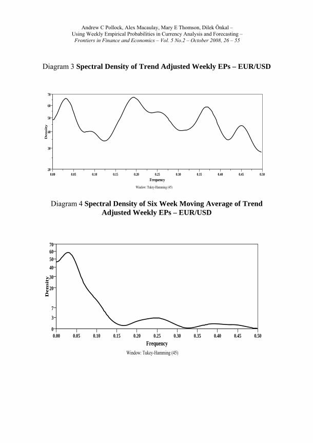
Spectral analysis, using the SPSS package, was applied to the trend adjusted EP using the spectral density estimates smoothed with window spans of various lengths. Diagram 3 presents the results for the spectral density using the Tukey-Hamming window with a span of 45.

While the spectral density shows an irregular pattern, there are two peaks with relatively high power. One occurs at frequency 0.19 which would indicate a cycle of approximately 5 weeks or 25 trading days. This would be consistent with tertiary trends lasting on average 2.5 weeks or 13 trading days. The other occurs at frequency 0.035 which would indicate a cycle of an approximate length of 28 weeks or 140 trading days. This would be consistent with secondary trends averaging 14 weeks or 70 trading days. The spectral density plot, however, indicates a smaller peak at the 0.38 frequency but this could just reflect harmonic influences from the 0.19 frequency cycle.

To remove high frequency variation caused by tertiary trends a six week moving average of the weekly EPs was used to allow concentration on the secondary trends. Diagram 4 shows the effect of filtering on the spectral density by applying a six week moving average to the EPs. A clear peak now occurs at the 0.035 frequency with the power at higher frequencies considerably reduced. This more clearly highlights the importance of secondary trends in the EUR/USD exchange rate.

4.5 Empirical probability predictions

The weekly (non-overlapping) EP predictions (for Wednesdays) for

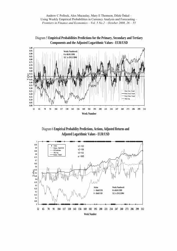
the primary, secondary and tertiary components were obtained using the procedure set out in sub-section 3.2. The lengths of the moving periods used (n1, n2 and n3) were 60 weeks, 6 weeks and 1 week respectively. Plots of these series are presented in Diagram 5 together with a plot of the logarithms of the EUR/USD (scaled to lie between zero and unity). The logarithms of the actual series showed the declining primary trend prior to week 90 which showed a decline in momentum between weeks 90 and 170. Around week 170 a clear upward primary trend began which lasted until the end of the period. The plot of the predicted primary component EPs shows the primary trend pattern with values below 0.5 until week 176 after which the values were above 0.5. The relative height of peak in the EPs illustrated the strong primary trend in


the third quarter of the period as well as identifying a marked fall in momentum between weeks 260 and 290. The plot of the predicted secondary component EPs highlights the secondary trend patterns, with variable lengths, in the actual (logarithms) of the EUR/USD, allowing secondary trends to be much easier to identify. The EPs plainly show the strength of each trend as indicated by the height of the peaks and troughs. The decline from a peak or rise from a trough reflected the weakening trend momentum. Values above 0.5 indicate that the average weekly changes (in logarithms) are positive, consistent with an upward trend, and values below 0.5 indicates the average changes are negative, consistent with a downward trend. The secondary component EPs generally showed a peak or trough in advance of the secondary trend changes in the actual (logarithms) series illustrating the major advantage of using this measure in the identification of secondary cycles, momentum and trend reversals that clearly distinguished secondary trends from the primary trend. The relative height of peaks and troughs in the EPs illustrated the strong primary trend in the third quarter of the period as well as identifying a marked fall in momentum between weeks 260 and 290. The plot of the predicted tertiary component EPs showed considerable volatility reflecting the nature of tertiary trends. The plot shows that they quickly fall back (rise) after a high (low) value had occurred. In making one week ahead predictions the tertiary EPs can, therefore, be an important factor when combined with the primary and secondary component EPs.

These EP component predictions were then combined to form one week ahead EP predictions for the various values of the model set out in sub-section 3.3 for the assigned range of values 1v , 2v and 3v .That is: 1v = 0, 0.1,

0.2, 0.3 or 0.4; 2v = 0.6, 0.7, 0.8, 0.9 or 1; 3v = 0, 0.1, 0.2, 0.3 or 0.4, with

321 vvv = 1. These EP predictions are presented in Diagram 6 using, as an

example, the values 1v = 0.3, 2v = 0.6 and 3v = 0.1. The graph illustrates that the

EP predictions clearly show secondary trend cycles with variable periods. A plot of the logarithms of the actual series (adjusted to values between zero and unity) is also presented. The EP predictions show a similar pattern to the secondary component predicted EPs. This is not surprising given that 60% of the weight is assigned to the secondary trend. The predicted EPs do not, however, have such sharp peaks and troughs reflecting the inclusion, albeit with a smaller weight, of the primary (30%) and tertiary (10%) predicted EP components in the model.

The analysis was repeated for the EPs obtained for Mondays,


Tuesdays, Thursdays and Fridays. The corresponding results are not presented here, but, as would be expected, reflected similar characteristics to the Wednesday values.

4.6 Results from the trading investment model

The trading/investment model was applied to the weekly (5 day)

predictions for the EPs to generate action decisions (i.e., hold all assets in EUR or USDs) using the procedure set out in sub-section 3.5. Four different values of the parameter, α, were used: 0, 0.05, 0.1 and 0.15.

To illustrate the application of the procedure, it is assumed that a hypothetical US investor holds all assets in USDs or EURs. It is further assumed, for convenience, that the interest rate on EUR and USD assets are identical and there are no transaction costs. The data period used as a basic input extends from 22/03/00 (week 63) to 29/12/04 (week 312). The first decision day is 15/03/00 (week 62), with the decision implemented at the quote on that day and profitability of the action calculated on 22/03/00 (week 63).

Suppose the US investor starts with a defined unit of USDs at week 61 (day 307), 0A , in equation (9) and we use weeks k = 62 to 312 (i.e., days

317 to 1562) to calculate the return. For simplicity, 0A can be set as unity. If

the investor had kept this amount in USDs over the whole period, zero profit would have been made (assuming that interest payments are excluded), that is, neither a profit nor loss on holding USD. Thus id = 0 for all i in equation (9)

so that kA = 0A =1 for all k, k = 62 to 312. On the other hand, if the capital had

been held in EURs over the whole period then id = 1 throughout in equation

(9) and the capital would be valued at 1.4074 units of USDs; a profit of 0.4074 units of USDs over the whole period or a profit of 0.163% in USDs per trading week.

Now consider the investor who follows a simple trading system based on the five day predicted EPs using the decision criteria set out in sub-section 3.5 which involves holding either EURs or USDs. For example, using the model specification, 1v = 0.3, 2v = 0.6, and 3v = 0.1 and action specification

α = 0.05 (the best performing specifications), id would take a value of unity or

zero determined by the action criteria. The return for holding EURs for the


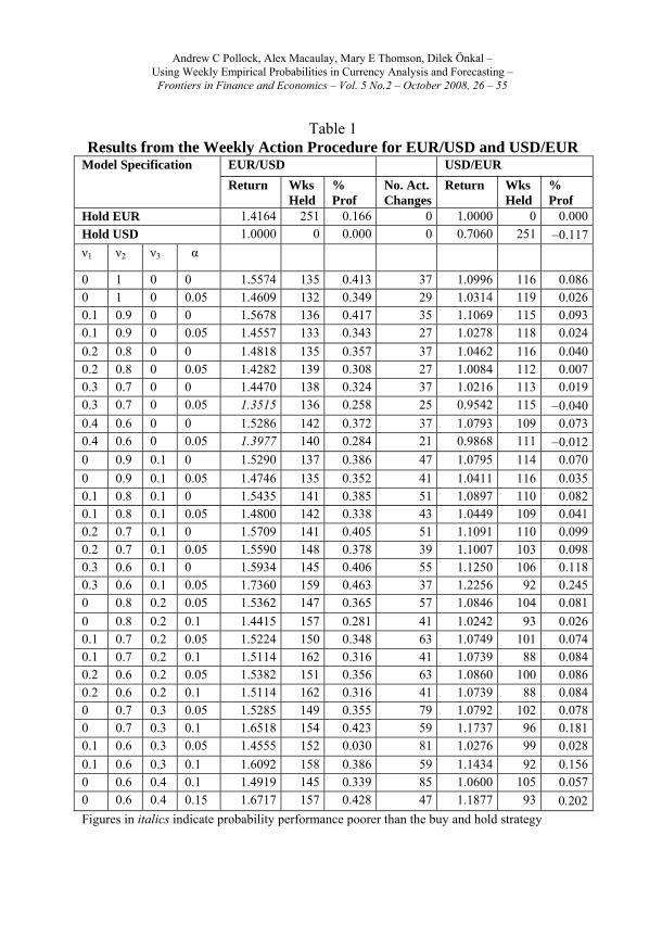
whole period (adjusted to a 0.5 unit starting value for better graphical presentation) is presented together with the return from the model/strategy set out above in Diagram 6. Diagram 6 clearly shows that this model/strategy consistently performed better than the ‘hold EURs’ strategy over the period. The action plot shows weeks when either the EURs (value unity) or the USD (value zero) were held. This clearly shows that ‘hold EUR’ actions dominated after week 170. Table 1 sets out the return over the whole period, the number of weeks held, the percentage profit for weeks and the number of action changes made for the various values within the defined range of specifications for 1v , 2v , 3v and α for the EUR/USD. In addition, the values of α were set at

0 or 0.05 when 3v was 0 or 0.1, the values α were set at 0.05 or 0.1 when 3v was 0.2 or 0.3 and the values α were set at 0.1 or 0.15 when 3v was 0.4. This

is consistent with the points made in sub-section 3.3. The table shows that for the defined specification (i.e., 1v = 0.3, 2v = 0.6, 3v =0.1 and α = 0.05) the total

return at the end of the period would be 1.7360 units USDs with EURs held for 159 weeks out of the total of 251 weeks. This would have resulted in a profit per week over the whole 251 week period of 0.293%. It is, however, appropriate to calculate the profit only over the days when EURs were held as an astute trader/investor would look for other potential profit opportunities for the USD assets when EURs were not held. In practice, it is likely that the trading/investment strategy would be integrated with similar strategies across a wide range of USD currency pairs. The percentage profit per week given in Table 1 is, therefore, 0.463% with regard to USDs which only relates to days when EURs were held. This can be compared with 0.166% from the hold EUR strategy (for all 251 weeks). The profit per week when EURs were held is almost treble that of the ‘hold EURs only’ strategy.

The effective evaluation of a currency trading/investment system also requires consideration of the USD/EUR from the viewpoint of a European investor holding EURs or USDs. Table 1 also presents similar figures in terms of the USD/EUR. For instance, using the model specification set out above the results the return was 1.2256 EUR compared with the hold USDs return of only 0.7060 EUR such that the hold USDs strategy resulted in a loss per week for the whole period of 0.117% per week whereas the trading system would have resulted in a profit of 0.246% per week (when USD held, i.e., 92 out of the total of 251 weeks). In fact, the percentage profit on all model specifications of the trading/investment system appear to be higher than the


always hold foreign currency case for all specifications of 1v , 2v , 3v and α in

all cases for both the EUR/USD and USD/EUR. The return over the period was higher for all model specifications of the USD/EUR and in all but two cases for the EUR/USD. It is also interesting to note that not only was the return over the whole period for the USD/EUR actions higher in all cases than the ‘always hold USD’ strategy but only two specifications of the returns on the USD/EUR actions were less than unity.

In the application of the above transaction costs and interest rate differentials were not included in the procedure. Transactions costs and interest rate differentials can be quite variable in their effect on different traders/investors in different situations (e.g., with respect to volumes of assets managed). Interest rate differentials may be viewed, however, as being important as over the period under consideration the differential was in favour of the USD in the first part of the period when the EUR was depreciating and in favour of the EUR in the second part of the period when the EUR was appreciating. This would have had some impact on percentage profitability of actions as the procedure suggested predominantly holding the currency that had the lower interest rate. The interest rate differential, although being quite variable, was, in general, not very large, with the differential rate per annum lower than 3% with 1% being more typical. Given the relative low interest differentials between the EURs and USDs and relative small transaction costs involved it can be concluded that the results set out in Table 1 would only marginally be affected by these additional costs.

The above illustrates that this fairly straightforward application of the weekly EP trading system can be very effective and can have considerable potential as a basis for developing a trading/investment system. This system could be easily extended to incorporate the role of human judgement in the process of the choice of action decisions. For instance, action decisions could be examined with reference to the actual level of the predicted EP to directly incorporate a measure of confidence with which the action would be held. For example, there would be much greater confidence in action decisions to hold EURs when the predicted EPs have values above 0.7 than when they have values below 0.6. A graph similar to Diagram 6 could be used to incorporate judgement into the trading/investment system that would then generate potential action decisions combined with the predicted EPs. 5 - Conclusion

It is shown that weekly EP predictions can be used to identify trends


in exchange rates that incorporate information regarding momentum, thus facilitating the identification of relevant trend changes. These predictions can then be used to aid in the process of generating buy or sell signals in a profitability context. These EPs measure the strength and momentum of market movements in an integrated form that has considerable advantages over traditional analysis momentum indicators. Furthermore, as EPs are derived from a statistically formulated framework based on the Normal distribution and exchange rate behaviour, they do not suffer from the problem often associated with mechanical technical analysis tools that may portray ad-hoc measures of chartist concepts. The EP procedure offers considerable practical applications to the development of trading/investment systems, as the procedure provides not only buy and sell indications but also gives directional probabilities associated with the identified actions.

In the application of the EP procedure it is desirable to have identifiable cycles present. The changes in the logarithms of the EUR/USD for a six year period (04/01/99 to 31/12/04) used in this study gave spectral density estimates consistent with tertiary and secondary cycles. The profit returns from a range of model specifications were considerably higher than the hold one currency benchmark action. The time period used for this analysis can easily be extended as the available data expands over time. The procedure can also be applied to other exchange rates and over different time periods. The authors found (but not presented here) that cycles are, in general, a feature of currency pairs involving the USD. While the procedure as it stands would, generally, be applicable to USD exchange rates, which accounted for 90% of the global foreign exchange market turnover in 2004 [Bank for International Settlements, 2005], some modifications are likely to be required for other non-USD currency pairs. Non-USD rates are likely to reflect combined cycle influences generated from their related USD pairs. In a more general application of the EP procedure to other exchange rates (or indeed other financial instruments) and time periods it would be required to experiment with various model parameters and to check the validity of the Normality assumption.

In practice, the EP procedure can be more effectively used on a subjective basis when combined with information from the original series or, for example, technical analysis indicators. This could be utilized to provide a trading/investment system that would integrate the model with judgement resulting in integrated action decisions. The use of the model in a trading/investment environment could be more effective with judgemental


revisions (with additional technical analysis or statistical input) to the model parameters on a weekly basis in response to market events. The effectiveness of such a combined mechanical/subjective trading system could be evaluated using the profit benchmarking illustrated above. Furthermore, the EP predictions could be evaluated using a procedure that incorporates probability accuracy analysis based on ex-post realised EPs [Pollock et al, 2005]. In this way, as well as with relative percentage profit figures, measures of overall performance could be obtained and the accuracy components may be decomposed to reveal different aspects of accuracy performance. This would be particularly important where judgement is structurally integrated into the mechanical procedures, providing critical feedback regarding analyst performance that could be used to improve on the accuracy of currency analysts in their trading/investment recommendations.

The fact that the procedure provides probabilities for associated actions has further potential for extending this procedure. In practice, a trader/investor would probably consider a range of currency pairs in relation to a specific currency. The EP predictions can, for example, provide a mechanism to choose between actions for a set of USD rates such as implementing a buy action for the currency with the highest EP at a given time. This procedure could be further expanded using predicted EPs derived from a method that ensures consistent predictions when multiple related currency pairs are used [extending the procedure set out in Pollock et al, 2002]. Such potential extensions of current work highlight the significance of the proposed technique in providing an effective support tool to aid the financial agents operating in a global fusion of financial markets.

References

Anderson, T.W. and D.A. Darling, 1954. A test of goodness-of-fit. Journal of

the American Statistical Association, 49, 765769. Bank for International Settlements. 2005. Foreign Exchange and Derivative

Market Activity in 2004. Basel, Switzerland. (Downloadable from website http://www.bis.org/publ/rpx05t.pdf).

Bartlett, M.S., 1946. On the theoretical specification of sampling properties of autocorrelated time series. Journal of the Royal Statistical Society, Series B, 8, 2741.

Cheung, YM. and M.D. Chinn, 2001. Currency traders and exchange rate


dynamics: a survey of the US market. Journal of International Money and Finance, 20, 439471.

Cooper, M.J., R.C. Gutierrrez Jr. and A. Hameed, 2004. Market shares and momentum. The Journal of Finance, 59, 1345-1365.

Evans, M.D.D. and R.K. Lyons, 2003. How is macroeconomic news transmitted to exchange rates? Working Paper No: 9433, NBER.

Froot, K.A. and T. Ramadorai, 2005. Currency returns, intrinsic value and international-investor funds. The Journal of Finance, 60, 1535-1566.

Harvey, A.C., 1993. Time Series Model. (Harvester Wheatsheaf, New York). Hsieh, D.A., 1988. The statistical properties of daily foreign exchange rates:

19741993, Journal of International Economics, 24, 129145. Jagadeesh, N. and S. Titman, 2001. Profitability of momentum strategies: an

evaluation of alternative explanations. The Journal of Finance, 56, 699-720.

Jaffe, J. and R. Westerfield, 1985. The week-end effect in common stock returns: international evidence. The Journal of Finance, 40; 433454.

Kamara, A., 1997. New evidence on the Monday seasonal on stock returns, The Journal of Business, 70; 6384.

Lakonishok, J. and S. Smidt, 1988. Are seasonal anomalies real? A ninety-year perspective. Review of Financial Studies, 1; 403-425.

Larson, S.J. and J. Madura, 2001. Overreaction and underreaction in the foreign exchange market. Global Finance Journal, 12, 153177.

McFarland, J.W., R.R. Pettit and S.K. Sung, 1982. The distribution of foreign exchange price changes: trading day effects and risk measurement. Journal of Finance, 37, 693715.

Murphy, J.J., (1999). The Technical Analysis of Financial Markets. (New York Institute of Finance, Paramus, New Jersey).

Nelson, C.R. and C.I. Plosser, 1982. Trends and random walks in macroeconomic time series: some evidence and implications. Journal of Monetary Economics, 10, 139162.

Nelson, S.A., 1903. ABC of Stock Market Speculation. (Reprinted by Omnigraphics, Griswold, Detroit, 1989).

Pollock, A.C., A. Macaulay, D. Önkal-Atay and M.E. Thomson, 2002. Consistent probability currency predictions between related cross

rates. In K.D. Lawrence, M.D.Geurts, and J.G. Guerard Jr. (eds.). Advances in Business and Management Forecasting, Volume 3. (JAI, Oxford, 161-175).

Pollock, A.C., A. Macaulay, M.E. Thomson and D. Önkal, 2004. Short term


empirical directional probabilities for daily exchange rate movements. Paper presented at the 34th Meeting of the Euro Working Group on Financial Modelling, Paris.

Pollock, A.C., A. Macaulay, M.E. Thomson and D. Önkal, 2005. Performance evaluation of judgemental directional exchange rate predictions. International Journal of Forecasting, 21, 473489.

Seier, E., 2002. Comparison tests for univariate Normality. Discussion Paper, Department of Mathematics, East Tennesse State University, Johnson City (Downloadable from website http://interstat.stat.vt.edu/interstat/articles/2002/articles/J02001.pdf).

Taylor, M.P., and H. Allen, 1992. The use of technical analysis in the foreign exchange market. Journal of International Money and Finance. 11, 30431


Table 1 Results from the Weekly Action Procedure for EUR/USD and USD/EUR

EUR/USD USD/EUR Model Specification

Return Wks Held

% Prof

No. Act. Changes

Return Wks Held

% Prof

Hold EUR 1.4164 251 0.166 0 1.0000 0 0.000

Hold USD 1.0000 0 0.000 0 0.7060 251 0.117 ν1

ν2 ν3

α

0 1 0 0 1.5574 135 0.413 37 1.0996 116 0.086 0 1 0 0.05 1.4609 132 0.349 29 1.0314 119 0.026 0.1 0.9 0 0 1.5678 136 0.417 35 1.1069 115 0.093 0.1 0.9 0 0.05 1.4557 133 0.343 27 1.0278 118 0.024

0.2 0.8 0 0 1.4818 135 0.357 37 1.0462 116 0.040 0.2 0.8 0 0.05 1.4282 139 0.308 27 1.0084 112 0.007 0.3 0.7 0 0 1.4470 138 0.324 37 1.0216 113 0.019 0.3 0.7 0 0.05 1.3515 136 0.258 25 0.9542 115 0.040 0.4 0.6 0 0 1.5286 142 0.372 37 1.0793 109 0.073 0.4 0.6 0 0.05 1.3977 140 0.284 21 0.9868 111 0.012 0 0.9 0.1 0 1.5290 137 0.386 47 1.0795 114 0.070

0 0.9 0.1 0.05 1.4746 135 0.352 41 1.0411 116 0.035 0.1 0.8 0.1 0 1.5435 141 0.385 51 1.0897 110 0.082 0.1 0.8 0.1 0.05 1.4800 142 0.338 43 1.0449 109 0.041 0.2 0.7 0.1 0 1.5709 141 0.405 51 1.1091 110 0.099 0.2 0.7 0.1 0.05 1.5590 148 0.378 39 1.1007 103 0.098 0.3 0.6 0.1 0 1.5934 145 0.406 55 1.1250 106 0.118 0.3 0.6 0.1 0.05 1.7360 159 0.463 37 1.2256 92 0.245 0 0.8 0.2 0.05 1.5362 147 0.365 57 1.0846 104 0.081

0 0.8 0.2 0.1 1.4415 157 0.281 41 1.0242 93 0.026 0.1 0.7 0.2 0.05 1.5224 150 0.348 63 1.0749 101 0.074 0.1 0.7 0.2 0.1 1.5114 162 0.316 41 1.0739 88 0.084 0.2 0.6 0.2 0.05 1.5382 151 0.356 63 1.0860 100 0.086 0.2 0.6 0.2 0.1 1.5114 162 0.316 41 1.0739 88 0.084 0 0.7 0.3 0.05 1.5285 149 0.355 79 1.0792 102 0.078 0 0.7 0.3 0.1 1.6518 154 0.423 59 1.1737 96 0.181 0.1 0.6 0.3 0.05 1.4555 152 0.030 81 1.0276 99 0.028

0.1 0.6 0.3 0.1 1.6092 158 0.386 59 1.1434 92 0.156 0 0.6 0.4 0.1 1.4919 145 0.339 85 1.0600 105 0.057 0 0.6 0.4 0.15 1.6717 157 0.428 47 1.1877 93

Figures in italics indicate probability performance poorer than the buy and hold strategy

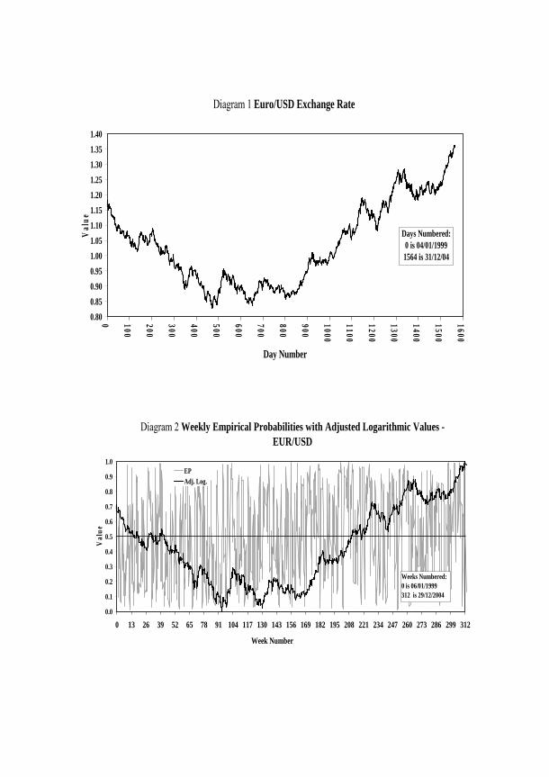
Diagram 1 Euro/USD Exchange Rate

0.80

0.85

0.90

0.95

1.00

1.05

1.10

1.15

1.20

1.25

1.30

1.35

1.40

0 100

200

300

400

500

600

700

800

900

1000

1100

1200

1300

1400

1500

1600

Day Number

Val

ue

Days Numbered:0 is 04/01/19991564 is 31/12/04

Diagram 2 Weekly Empirical Probabilities with Adjusted Logarithmic Values - EUR/USD

0.0

0.1

0.2

0.3

0.4

0.5

0.6

0.7

0.8

0.9

1.0

0 13 26 39 52 65 78 91 104 117 130 143 156 169 182 195 208 221 234 247 260 273 286 299 312

Week Number

Val

ue

EP

Adj. Log.

Weeks Numbered:0 is 06/01/1999 312 is 29/12/2004


Diagram 3 Spectral Density of Trend Adjusted Weekly EPs – EUR/USD

Frequency0.500.450.400.350.300.250.200.150.100.050.00

Den

sity

70

60

50

40

30

20

Window: Tukey-Hamming (45)

Diagram 4 Spectral Density of Six Week Moving Average of Trend Adjusted Weekly EPs – EUR/USD

Frequency0.500.450.400.350.300.250.200.150.100.050.00

Den

sity

7060

50

40

30

20

7

3

0

Window: Tukey-Hamming (45)


Diagram 5 Empirical Probabilities Predictions for the Primary, Secondary and Tertiary Components and the Adjusted Logarithmic Values - EUR/USD

0.000.050.100.150.200.250.300.350.400.450.500.550.600.650.700.750.800.850.900.951.00

52 65 78 91 104 117 130 143 156 169 182 195 208 221 234 247 260 273 286 299 312

Week Number

Val

ue

Pred. Tert. Trend

Pred. Secd. Trend

Pred. Prim. Trend

Adj. Log.


Diagram 6 Empirical Probability Predictions, Actions, Adjusted Returns and Adjusted Logarithmic Values - EUR/USD

0

0.05

0.1

0.15

0.2

0.25

0.3

0.35

0.4

0.45

0.5

0.55

0.6

0.65

0.7

0.75

0.8

0.85

0.9

0.95

1

52 65 78 91 104 117 130 143 156 169 182 195 208 221 234 247 260 273 286 299 312

Week Number

Val

ue

ActionReturn - Hold EUREP PredictionAdj. Log.Return - Model

v1 = 0.3v2 = 0.6v3 = 0.1 = 0.05

Action 1 - Hold EUR0 - Hold USD


Using Weekly Empirical Probabilities in Currency Analysis ... · Andrew C Pollock, Alex Macaulay,...

Documents

Transcript of Using Weekly Empirical Probabilities in Currency Analysis ... · Andrew C Pollock, Alex Macaulay,...