Using Visual Saliency and Geometric

Sensing for Mobile Robot Navigation

Kin-Leong HoSt Catherines’ College

DPhil Transfer ReportSupervised by Dr P.M Newman

Robotics Research GroupDept of Engineering Science

University of OxfordMichaelmas 2004

August 31, 2004

Abstract

Autonomous navigation of robots has been of immense research inter-ests since the beginning of robotics. The potential benefits of having a robotwith autonomous navigation capability are of immense value to the researchcommunity and the society at large. Much progress has been made in thearea but a fully functional autonomous navigation system has yet to be de-veloped.

The focus of this project is to develop a multi-sensorial system, which iscapable of achieving the synergy of combining and complementing geomet-rical information from a laser scanner and photometrical information from acamera. It is our belief that a navigational system based solely on one sen-sory information will be inadequate and an additional form of sensory data isrequired to enhance the robustness and reliability of the navigation system.Henceforth, a concept of local workspace descriptor is being developed. Alocal workspace descriptor is comprised of different sensor modalities thatdescribe the workspace the robot is currently in. A combination of sensormodalities such as local geometry, visual texture, visual features or robot’strajectories will form the local workspace descriptor. In particular, effortswill made to apply existing repertoire of computer vision tools to describethe local workspace.

The research will be focused on developing a toolkit of algorithms thatcan effectively select “interesting” landmarks in the environment, repre-sent the visual landmarks in distinctive and compact formats that can beeasily stored and compared with other visual landmarks. To develop thistoolkit, several existing computer vision algorithms such as Kadir/Bradyscale saliency algorithm, Matas’ maximally stable extremal regions, homog-raphy and Lowe’s scale invariant feature transform descriptors will be inves-tigated to determine their suitability for use in an indoor environment. Inaddition, the use of geometry obtained from the laser scanner will be usefulin simplifying the computer vision problems.

Contents

1 Introduction 51.1 Motivation for Autonomy . . . . . . . . . . . . . . . . . . . . 51.2 Current state of development in SLAM . . . . . . . . . . . . . 61.3 Research Objectives . . . . . . . . . . . . . . . . . . . . . . . 71.4 Proposed Methodology . . . . . . . . . . . . . . . . . . . . . . 8

2 Background - The SLAM Problem 92.1 Introduction to SLAM . . . . . . . . . . . . . . . . . . . . . . 92.2 Fundamentals . . . . . . . . . . . . . . . . . . . . . . . . . . . 92.3 Stochastic Mapping . . . . . . . . . . . . . . . . . . . . . . . 102.4 Extended Kalman filter . . . . . . . . . . . . . . . . . . . . . 132.5 Particle Filter . . . . . . . . . . . . . . . . . . . . . . . . . . . 152.6 Consistent Pose Estimate . . . . . . . . . . . . . . . . . . . . 15

3 Background - The Data Association Problem 173.1 Data Association . . . . . . . . . . . . . . . . . . . . . . . . . 17

3.1.1 “Nearest Neighbor” gating technique . . . . . . . . . . 183.1.2 Joint Compatibility Test . . . . . . . . . . . . . . . . . 20

3.2 Related Work . . . . . . . . . . . . . . . . . . . . . . . . . . . 21

4 Image Processing for Robust SLAM 244.1 Detection / Selection algorithm . . . . . . . . . . . . . . . . . 24

4.1.1 Understanding Saliency . . . . . . . . . . . . . . . . . 254.1.2 Using Saliency in SLAM . . . . . . . . . . . . . . . . . 274.1.3 Detection: Matas’s Maximally Stable Extremal Regions 30

4.2 Description: Scale Invariant Feature Transform . . . . . . . . 324.3 Matching of feature vectors . . . . . . . . . . . . . . . . . . . 344.4 Fusion of geometric and photometric information . . . . . . . 36

4.4.1 SICK LMS 200 Laser Scanner . . . . . . . . . . . . . . 36

1

4.4.2 EVI-D30 CCD camera . . . . . . . . . . . . . . . . . . 394.5 Homography . . . . . . . . . . . . . . . . . . . . . . . . . . . 41

4.5.1 Mathematical explanation of perspective transformation 414.5.2 Applying homographies to SLAM . . . . . . . . . . . . 43

4.6 Image Matching And View-based Recognition . . . . . . . . . 444.7 Image database and Image retrieval . . . . . . . . . . . . . . 47

5 Conclusions and Future Work 505.1 Research Schedule . . . . . . . . . . . . . . . . . . . . . . . . 51

2

List of Figures

1.1 Projection of robot’s path based on odometry . . . . . . . . . 6

2.1 A vehicle taking relative measurements to environment land-marks . . . . . . . . . . . . . . . . . . . . . . . . . . . . . . . 11

2.2 Consistent Pose Estimate . . . . . . . . . . . . . . . . . . . . 16

3.1 Simulation of SLAM with data association . . . . . . . . . . . 193.2 Corresponding Innovation plot for simulation of SLAM with

data association . . . . . . . . . . . . . . . . . . . . . . . . . . 20

4.1 Implementation of scale saliency algorithm . . . . . . . . . . . 264.2 Image from camera looking down the corridor . . . . . . . . . 274.3 Top 5 most salient regions out of all the possible salient re-

gions detected in 4.2 . . . . . . . . . . . . . . . . . . . . . . . 284.4 Salient regions on poster . . . . . . . . . . . . . . . . . . . . . 294.5 Image Sequence of viewpoints . . . . . . . . . . . . . . . . . . 304.6 Search space of pixel . . . . . . . . . . . . . . . . . . . . . . . 314.7 Grayscale level versus no. of pixels cumulative graph . . . . . 324.8 Implementation of Matas’ Maximally Stable Extremal Re-

gions Algorithm . . . . . . . . . . . . . . . . . . . . . . . . . . 334.9 SIFT Descriptor . . . . . . . . . . . . . . . . . . . . . . . . . 344.10 Features detected within image represented by SIFT keys . . 354.11 Different views of camera and laser scanner . . . . . . . . . . 364.12 2D Laser Scan of Ewert House Corridor . . . . . . . . . . . . 374.13 A line segmentation process of data points obtained from a

2D laser scanner . . . . . . . . . . . . . . . . . . . . . . . . . 384.14 Pinhole camera geometry . . . . . . . . . . . . . . . . . . . . 394.15 A typical calibration object: The Tsai Grid . . . . . . . . . . 404.16 Homography induced by a plane . . . . . . . . . . . . . . . . 414.17 Different viewpoints of poster . . . . . . . . . . . . . . . . . . 43

3

4.18 Matching frontal parallel image; Red circle represent salientregions that are common to images found in figure 4.17(b)and figure 4.17(d) . . . . . . . . . . . . . . . . . . . . . . . . . 44

4.19 Image matching with a different poster using stored featurevectors . . . . . . . . . . . . . . . . . . . . . . . . . . . . . . . 46

4.20 Architecture of a Content based Image Retrieval System: Ob-tained from [27] . . . . . . . . . . . . . . . . . . . . . . . . . . 47

4.21 Various forms of possible laser range scans . . . . . . . . . . . 49

5.1 Research timeline . . . . . . . . . . . . . . . . . . . . . . . . . 52

4

Chapter 1

Introduction

1.1 Motivation for Autonomy

This section explains why there is a need for an autonomous mobile robot.Starting from an unknown location in an unknown environment, an au-tonomous mobile robot will be able to incrementally build a map of theenvironment using only relative observations of the environment and thenuse this map to localize and navigate. It seems that most industrial roboticsproblems have been solved reasonably well by the creation of highly engi-neered environments for the robots to work within. For example, the GEC-caterpillar AGV uses a rotating laser to locate itself with respect to a set ofbar codes that are fixed at known location. [26] Similarly, the TRC corpo-ration has developed a localization system that make use of retro-reflectivestrips and ceiling lights as beacons that are observed by vision and activeinfrared sensors. This approach works well if the robots have to work ina static environments. However, problems arise when the robots have towork in dynamic environment that is constantly changing and they can nolonger rely on artificial infrastructure or prior topological knowledge of theenvironment.

Consider some scenarios when autonomy is required in order for robotsto successfully accomplish their mission:

• Autonomous exploration on the Mars surface

• Mine detection by autonomous underwater vehicle

• Search and Rescue in collapsed buildings

5

• Automobiles/Aircrafts/Ships traversing in heavy traffic on autopilotwith collision avoidance capability

• Aerial surveillance by aerial survey drones

• Mapping of ocean floor by autonomous underwater vehicle

1.2 Current state of development in SLAM

The underlying problem in developing an autonomous navigation system isthe general problem of simultaneously localizing and mapping with uncer-tain sensory data. Without a precise map, the robot cannot localize itselfusing the map. On the other hand, without precise knowledge of its loca-tion, the robot cannot build a representation of its environment. As separateproblems, the localization problem [20] and the mapping problem [21] are

−40 −30 −20 −10 0 10 20 30 40 50 60−60

−40

−20

0

20

40

60

Figure 1.1: The above figure illustrates what the path of the robot will looklike based solely on odometry after a robot moves round a hallway in EwertHouse and return to its original position. It can be seen that the startposition and estimated end position are not the same

6

well understood.

The work done by Smith, Self and Cheeseman [33] paved the way forthe research in simultaneous localization and mapping (SLAM). Smith, Selfand Cheeseman used a Kalman filter to estimate a large state vector com-prised of a vehicle’s location and orientation and the map - a set of featureparameterizations.

Much research on SLAM has focused on the map-scaling problem: asthe number of features stored in the state vector increases, the computa-tional cost of updating the correlations between the state estimates increasesquadratically. It severely limits the ability of the robot to map large areas ofthe environment due to computation time. New efficient frameworks such asFastSLAM [28], Atlas [2] and Constant-time SLAM [31] have been proposedas potential solutions. These have helped to reduce the computation effortfrom O(n2) to O(m log n) to O(1).

Nevertheless, all these state estimation frameworks are still susceptibleto the data association problem. Data association remains one of the keychallenges in solving the general SLAM problem. Data association is theprocess of corresponding data measurements with the representation of theenvironment. An efficient data association scheme must be able to correctlyassign measurements with currently stored features, distinguish false alarmsand detect new feature. Any incorrect assignment will result in the map toconverge to the wrong state. Data association techniques such as Joint Com-patibility Testing [29] and Multi-target tracking [32] have been developedto enhance discrimination and reliability over the classical nearest neighborgating technique. These data association techniques will be discussed ingreater details in later chapters.

1.3 Research Objectives

The focus of this research is to tackle the data association problem. Themain approach taken is to take advantage of the different modalities of dif-ferent sensors; laser range and camera images in this case. As in existingimplementations, our robot will continue to navigate using sensor data pro-vided by the laser scanner. However, it has the additional discriminativepower of computer vision. The robot will be able to redetermine its loca-tion within an environment it has mapped by matching the present image

7

it captures with the database of images it has captured and stored previ-ously when it navigates around the environment. The laser scanner and thecamera are not working as two separate system but will be combined towork in tandem and to complement each other. Previous data associationtechniques have continued to rely on a single source of sensory data to buildthe map and localize the robot and at the same time use the same sensoryinput to discriminate among similar features in cluttered environment.

1.4 Proposed Methodology

One of the fundamental reasons why current data association techniques failis because these techniques rely solely on geometry. An natural extensionto current data association techniques will be to add more sensor modalitiessuch as texture for discernment. For instance, texture will enable the robotto distinguish a red brick wall versus a brown wooden door. In addition,visually interesting landmarks can be used to mark the local workspace.Consider a robot traversing down a long corridor, the local workspace de-scriptor will consist of geometry describing the workspace to be a corridor,texture information of the surroundings and visual salient landmarks in thatworkspace. The visual salient landmark can easily be a poster in the corridordetected by our selector as the most interesting landmark in the environ-ment comprised mainly of walls and doors. In order to determine that thelandmark is visually wide baseline salient, the robot will only select thelandmark if it remains visually salient from different viewpoints. An im-age of the poster will be captured. Interesting features of the image willbe detected and described distinctively by feature vectors. The next timethe robot traverses through the same area of the corridor, the robot willpick up the same visual salient landmark, compare it with the database oflandmarks it has stored and realize that it has been through this area beforewithout relying solely geometric information.

8

Chapter 2

Background - The SLAMProblem

2.1 Introduction to SLAM

In order for a mobile robot to be truly autonomous, it must have the ca-pability to navigate in uncharted and unknown environment. This meansthat it must be able to actively sense the environment and build a repre-sentation of the environment, from which the robot can navigate with. Thisis the problem of simultaneous localization and mapping (SLAM). This isan inherently difficult problem due to the problem of uncertainty in mea-surements of sensors. It has been successfully demonstrated the problemof localization with a known map and the problem of map-building withperfect knowledge of pose of the vehicle as separate problems can be solved.However, to simultaneously solve the problems of localization and mappingis much more complex since the uncertainty from pose and measurementscompound each other. The estimation -theoretic foundation of this problemwas started with the seminal paper of [33], which describes a representationfor spatial information, called the stochastic map.

2.2 Fundamentals

In the Bayesian approach, one starts with the prior knowledge of the pa-rameter ρ(θ) which one can obtain its posterior pdf ρ(θ|z) using Bayes’s

9

formula:ρ(θ|z) =

ρ(z|θ)ρ(θ)ρ(z)

=1cρ(z|θ)ρ(θ) (2.1)

where c is the normalization constant, z is the measurement and θ is thestate derived from the measurements .

Maximum Likelihood Estimate is used when there is no prior knowledgeof the pose parameters. Therefore, the best estimate is the one that matchesmost closely with the measurement.

θ̂MLE = arg maxθ

ρ(z |θ) (2.2)

The maximum a-posteriori (MAP) estimator - MAP finds the value ofθ which maximizes the posterior distribution. The MAP estimator is usedwhen we have prior knowledge of the pose parameters. The best estimate isthe one which agrees most closely with the measurement and prior knowl-edge. When using the Bayes’ formula, the normalizing constant is droppedsince it is irrelevant for the maximization.

θ̂MAP = arg maxθ

ρ(z |θ)ρ(θ) (2.3)

The MAP estimator for a purely gaussian problem can be seen as aweighted combination of the MLE and the peak of the prior pdf of theparameter to be estimated, where the weightings of the prior pdf and themeasurements are inversely proportional to their variances.

Returning to the mobile robotics domain, starting with a robot possess-ing a sensor capable of producing at time, k, measurements zk, which area function of the pose, xk and its surroundings, M. The distribution of z ismodelled as a conditional density on x and M: ρ(z|x,M). The state of theworld, M, and the vehicle pose, xk, are to be derived from the conversion ofthis likelihood given all observations until time k.

ρ(xk,M |zk) = ρ(zk|xk,M)ρ(x,M |zk−1) (2.4)

2.3 Stochastic Mapping

Stochastic mapping obtains sufficient accuracy by combining uncertain in-formation from many sensor data: uncertain spatial relationships will be tied

10

Figure 2.1: In feature based SLAM, a vehicle takes relative measurementsto environment landmarks and makes use of these relative measurements toestimate the locations of the environment landmarks and its own locationin a global coordinates frame

up together in a representation that contains estimates of spatial relation-ships, their uncertainties and their interdependencies. Stochastic mappingallows the size of the state vector to vary as new features are added and oldfeatures are deleted.

The position and orientation of a mobile robot can be described by its co-ordinates , xv and yv, in a two dimensional cartesian reference and by itsorientation, φv, given as a rotation about the z axis:

xv =

xv

yv

φv

(2.5)

11

The stochastic map vector x with n features can be expressed as:

x =

xv

xf,1

xf,2...

xf,n

(2.6)

The system covariance matrix, P(x):

P(x) =

P(xv) P(xv,x1) . . . P(xv ,xn)

P(x1,xv) P(x1) . . . P(xv ,xn)

. . . . . .. . . . . .

P(xn,xv) P(xn),x1. . . P(xn)

(2.7)

The off-diagonal sub matrices encode the dependencies between the esti-mates of the different spatial relationships and provide the mechanism forupdating all the relational estimates.

The overall pdf is a gaussian distribution of N(x, P ).

Between state k−1 and k, no measurements of external features are made.The new state is predicted only by the process model, f, as a function of theold state and any control signal, u(k), applied in the process.

x̂(k|k− 1) = f(x̂(k− 1|k− 1), u(k), k) (2.8)

where x̂(k|k− 1) is the estimate of x at time k given first k− 1 measure-ment.

The control signal, u(k), is a function of the intended control signalun(k), and a zero mean gaussian distributed noise vector, v(k)

u(k) = un(k) + v(k) (2.9)

12

The predicted covariance is:

P (k|k− 1) = ∇FxP (k− 1|k− 1)∇F Tx +∇GvQ∇GT

v (2.10)

where ∇Fx:

∇Fx =

∂f1

∂x1. . . ∂f1

∂xm...

. . ....

∂fn

∂x1. . . ∂fn

∂xm

(2.11)

The measurement, z, is described as a function of, h, of the state vectorand a zero mean gaussian distributed noise vector.

z = h(x) + v (2.12)

where h defines the non-linear coordinate transform from state to observa-tion coordinates.

2.4 Extended Kalman filter

The Kalman filter provides a recursive bayesian estimator to the navigationproblems and can be easily applied to the new problems. It concurrentlyprovides a consistent estimates of uncertainty of the robot’s and the featurelandmarks’ positions based on predictive model of the robot’s motion andthe relative observation of the feature landmarks.

Kalman filter:New state estimate, x̂:

x̂(k|k) = x̂(k|k− 1) +W ν(k) (2.13)

13

New covariance estimate, P̂ :

P̂ (k|k) = P̂ (k|k− 1)−WSWT (2.14)

Innovation, ν:ν(k) = z(k)− z(k|k− 1) (2.15)

Kalman gain, W:W = P (k|k− 1)∇HT

x S−1 (2.16)

Innovation covariance, S:

S = ∇HxP (k|k− 1)∇HTx + R (2.17)

∇Fx =∂f

∂x=

∂f1

∂x1. . . ∂f1

∂xm...

...∂fn

∂x1. . . ∂fn

∂xm

(2.18)

∇Hx =∂h

∂x=

∂h1∂x1

. . . ∂h1∂xm

......

∂hn∂x1

. . . ∂hn∂xm

(2.19)

However, the use of the full map covariance at each step results in sub-stantial computational cost as the number of features stored in the mapincreases. As the number of features, n, increases, the computation in-creases as n2.

Also, the extended Kalman filter can only maintain one hypothesis withits unimodal Gaussian distribution. Therefore, one wrong data associationat one time step will lead to error in localization and mapping in consequenttime steps and the extended Kalman filter will not be able to recover fromit.

14

2.5 Particle Filter

In [28], an estimation technique called FastSLAM which integrates particlefilter and Kalman filter is presented to solve the Simultaneous Localizationand Mapping problem. Each particle consists of the estimate of the presentvehicle pose, st, all the previous poses of the vehicle, st−1, and a set of Nindependent Kalman filters for each feature which estimate feature locationassociated with each vehicle pose. It exploits the SLAM structure propertythat the feature estimates are conditional independent given the robot path.Therefore, if the correct path of the robot is known, the errors of the featureestimates will be independent of each other.

Given the stated independence of individual feature estimation due toknowledge of robot path:

ρ(M |st, nt, zt) =NΠ

n=1ρ(θn|st, nt, zt) (2.20)

where M is the map, st is all the poses till time t, nt is all the correspondenceof measurements to features till time t, zt is all the measurements till timet and θn is the nth feature.

The FastSLAM algorithm does not face the limitations of the extendedKalman filter, namely quadratic scaling of computation and unimodal Gaus-sian distribution. Computationally wise, FastSLAM is a O(m log(n)) prob-lem, where m is the number of particles and n is the number of featuresstored. FastSLAM is capable of maintaining multiple data association hy-potheses at the same time because the posterior is represented by multipleparticles. The data association technique employed by FastSLAM is never-theless the same as other estimation-theoretic techniques such as the Kalmanfilter.

2.6 Consistent Pose Estimate

In contrast to feature based techniques, consistent pose estimate is a methodthat makes use of dense sensor data. The method is incremental and runs inconstant time independent of the size of the map [19]. Consistent pose esti-mate method builds the map by incremental scan matching. Scan matchingis the process of rotating and translating a range scan such that a maximaloverlap with the priori map is achieved [25]. Correspondingly, the pose and

15

odometry of the robot can be estimated through scan matching. The tech-nique places constraints between poses.

With respect to figure (2.2), the new pose will have a link to the previouspose based on odometry and to several of the previous poses based on scanoverlaps and the resultant scan matches. Therefore, a set of local scans canbe integrated into a map patch which can be used to find matches in theold map. This map patch technique is much more reliable than finding mapcorrelation using single scans. However, the loop closure is not real-timeas it is more computational intensive. The two key contributions of con-sistent pose estimation is the creation of local patches and the loop closureusing map patches for map correlations [17]. However, data association orthe equivalent of map correlation remains a key criteria for this method tofunction properly as the consistent pose estimate method will not be ableto recover from a false match.

Figure 2.2: Set of robot poses with constraints between poses and mapobtained from consistent pose estimation [19]

16

Chapter 3

Background - The DataAssociation Problem

3.1 Data Association

Data association is the process of determining whether the existing worldrepresentation explains the measurement. If the existing world representa-tion does not explain the measurement, a check has to be made to deter-mine if the measurement is spurious. If the measurement is spurious, themeasurement is rejected. Otherwise, the world representation will have toaugmented using the measurement. In the specific case of feature basednavigation, data association is the task of considering whether if any of theexisting geometric parameter features explain the measurement. Correctdata association is crucial because an incorrect assignment will cause loca-tion estimation methods such as the extended Kalman filter to diverge.

The following two subsections describe current data association tech-niques, namely the nearest neighbor gating technique and the joint compat-ibility test. However, all these techniques relies on the observations froma single sensory data to try to solve the data association problem. Con-sequently, the actions of sensing the environment and distinguishing thedifferent features in the environment are solely dependent on a single formobservation.

17

3.1.1 “Nearest Neighbor” gating technique

For each feature in the vehicle state vector, predicted range and bearingmeasurements from the vehicle are generated. These predicted measure-ments are used to compare with the actual range and bearing measurementsfrom the sensor, using a weighted statistical distance in measurement space.Depending on the degrees of freedom, n, the probability of the chi-squaredensity can be looked up from the probability table for different confidencelevels. For this particular case where n is equal to 2 for range and bearing,γ is determined to be 9.21 in order to achieve a 99 percent certainty. Thefeature with the closest predicted measurements within the gate defined bythe Mahalanobis distance will be determined as the origin of the sensor mea-surement. If the sensor measurement does not gate with any of the mappedfeatures, a new feature will be initialized.

ν[k]T S−1ν[k] ≤ γ (3.1)

where ν[k] is the innovation and S is the innovation covariance.

Figure 3.1 is a simulation of SLAM with data association based on the“nearest neighbor” gating technique. The robot’s true positions are repre-sented by the green crosses. The robot’s estimated positions are representedby green, blue and red ellipses.

The green ellipses represent the covariance matrices of the robot’s esti-mated positions when no feature was detected and the robot’s position wasestimated by the control signal. The blue ellipses represent the covariancematrices of the robot’s estimated positions when new features were detected.The red ellipses represent the covariance matrices of the robot’s estimatedpositions when mapped features were detected.

The point features are represented by red plus signs. The blue ellipsesrepresent the covariance matrices of the point features’s positions when thefeatures were first detected. The red ellipses represent the covariance ma-trices of the point features’s positions when the features were re-detected.

It can be observed that when no features are detected, the uncertaintyof the robot’s position increases as depicted the increasing size of the greenellipses. When a mapped feature is detected, the uncertainty of the robot’sposition dramatically decreases as depicted by the red ellipses.

18

−20 −15 −10 −5 0 5 10 15 20−20

−15

−10

−5

0

5

10

15

Figure 3.1: x= Robot’s true position⊗ = represents the covariance matrices of the robot’s estimated positionswhen no feature was detected and the robot’s position was estimated by thecontrol signal⊗= represents the covariance matrices of the robot’s estimated positionswhen new features were detected⊗ = represents the covariance matrices of the robot’s estimated positionswhen mapped features were detected+ = point features⊕ = represents the covariance matrices of the point features’s positions whenthe features were first detected⊕ represents the covariance matrices of the point features’s positions whenthe features were re-detected.

19

0 5 10 15 20 25 30 35 40−4

−3

−2

−1

0

1

2

3

4

Figure 3.2: This is a innovation plot for the simulation of SLAM for figure(3.1). It shows that the innovation is between the innovation covariancebounds of 2 sigma. The breaks in between the plot is due to the fact thatthere are certain time steps when the vehicle was unable to make any ob-servations.

Figure (3.2) illustrates the plot of innovation versus time. The gaps ofin the plots are due to time steps when no features were detected. The redline depicts the outer limits of the innovation while the blue line depicts theactual innovation during each time step. It can be seen that the blue linelies within the outer bounds of the red lines. Therefore, the kalman filter isworking within specifications.

3.1.2 Joint Compatibility Test

However, there are limitations to the classical gated nearest neighbor ap-proach, which does not work well when the robot’s location uncertaintyis high or when there are many spurious measurements. A simple way toassure that resulting hypothesis contains jointly compatible pairings is touse a sequential compatibility nearest neighbor algorithm. It guaranteesthat all pairings belonging to the resulting hypothesis are jointly compati-ble. However, the sequential compatibility nearest neighbor algorithm mayaccept incorrect pairings. The joint compatibility test tackles this problemby measuring the joint compatibility of multiple matchings so as to removespurious matching.[29] The probability that a spurious pairing is jointly

20

compatible with all the number of pairings in the hypothesis is small. Thejoint compatibility test involves a search algorithm that traverse the inter-pretation tree in search of the hypothesis that have the largest number ofjointly compatible pairings.

3.2 Related Work

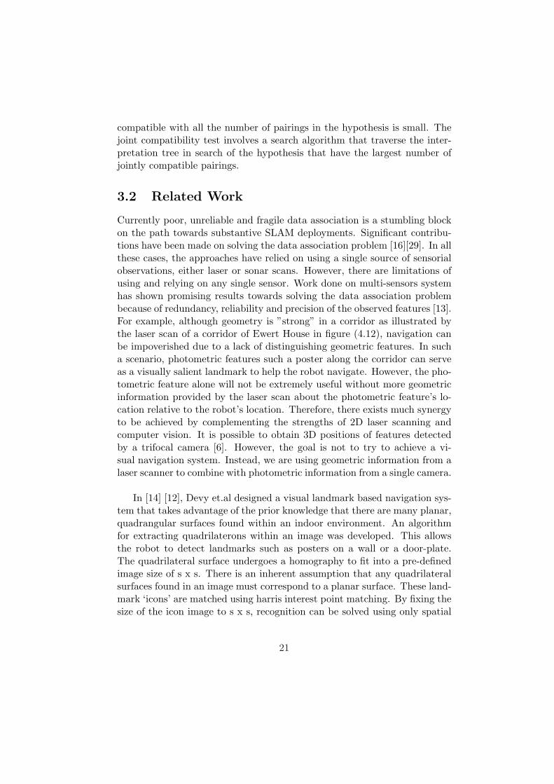
Currently poor, unreliable and fragile data association is a stumbling blockon the path towards substantive SLAM deployments. Significant contribu-tions have been made on solving the data association problem [16][29]. In allthese cases, the approaches have relied on using a single source of sensorialobservations, either laser or sonar scans. However, there are limitations ofusing and relying on any single sensor. Work done on multi-sensors systemhas shown promising results towards solving the data association problembecause of redundancy, reliability and precision of the observed features [13].For example, although geometry is ”strong” in a corridor as illustrated bythe laser scan of a corridor of Ewert House in figure (4.12), navigation canbe impoverished due to a lack of distinguishing geometric features. In sucha scenario, photometric features such a poster along the corridor can serveas a visually salient landmark to help the robot navigate. However, the pho-tometric feature alone will not be extremely useful without more geometricinformation provided by the laser scan about the photometric feature’s lo-cation relative to the robot’s location. Therefore, there exists much synergyto be achieved by complementing the strengths of 2D laser scanning andcomputer vision. It is possible to obtain 3D positions of features detectedby a trifocal camera [6]. However, the goal is not to try to achieve a vi-sual navigation system. Instead, we are using geometric information from alaser scanner to combine with photometric information from a single camera.

In [14] [12], Devy et.al designed a visual landmark based navigation sys-tem that takes advantage of the prior knowledge that there are many planar,quadrangular surfaces found within an indoor environment. An algorithmfor extracting quadrilaterons within an image was developed. This allowsthe robot to detect landmarks such as posters on a wall or a door-plate.The quadrilateral surface undergoes a homography to fit into a pre-definedimage size of s x s. There is an inherent assumption that any quadrilateralsurfaces found in an image must correspond to a planar surface. These land-mark ‘icons’ are matched using harris interest point matching. By fixing thesize of the icon image to s x s, recognition can be solved using only spatial

21

configuration of interests points, at only one scale and have an invariantrepresentation under perspective changes up to a certain level.

In [5], Ortin et.al have been demonstrated successfully that the first loca-tion problem can be solved using a combination of geometrical informationgathered by a 2D laser scanner and photometrical information gathered bya camera. A map composed of 8 observations of a 20x3 meters corridorwas used to successfully locate the robot. However, the observations weremanually selected. All the observations that were chosen were images of thewalls with posters. This is similar to our approach of visual saliency sinceintuitively, posters are most likely to be discriminative in a corridor of wallsand doors. Henceforth, an natural extension will be to design a selectionmechanism that will enable the robot to pick out visually salient landmarks,thereby removing the human from the decision-making loop. Furthermore,a 2D laser scanner is used to detect lines. The assumption is that these linesare part of a planar surface.

In [7], Fraundorfer and Bischof proposed to use natural, salient imagepatches as highly discriminative landmarks. In the experiment, data wascollected from 13 different locations of a hallway by taking images at differ-ent viewpoints for each location. Every location will now be represented bya small set of images and the experiment aims at recognizing the correct lo-cation by matching new views of location with the images in the training set.It should be pointed out that once again, there is no selection mechanismfor choosing a landmark to represent the location. Instead, a small randomset of images is used to represent each location. Local interest points basedon Harris corner detector are detected on the whole image. Areas of highinterest point concentration are detected by a graph based clustering algo-rithm. A local affine frame for every detected cluster is created to simplifyregion matching.

As evident by the recent research experiments, there is growing inter-est in applying computer vision in solving the data association problem inSLAM. Our approach varies from previous approaches in a few key points.Our approach is primarily a multi-sensorial approach which combines thesensor modalities of geometry and photometric information. A 3D laserscanner will be able to pick out planar surfaces from the environment withouthaving to make assumption that 2D lines form part of planar surfaces. A se-lection mechanism will be designed to pick out the visually salient landmarkautonomously versus the human-in-the-loop or random approach. Other

22

detection and description techniques such as Kadir/Timor scale saliency,Matas’ maximally stable extremal regions, Lowes’ scale invariant featuretransform algorithm will be investigated in this research to derive an efficientform of detecting and description of images that can be stored compactlyand matched effectively for the application of SLAM.

23

Chapter 4

Image Processing for RobustSLAM

In this chapter, various computer vision algorithms and techniques will bediscussed. A brief description of the theoretical underpinning of each ofthe algorithm will be given and a demonstration given on how each algo-rithm works. These algorithms and techniques have been selected based ontheir effectiveness and robustness in solving many computer vision prob-lems. Henceforth, the research will focus on how to apply these techniquesindividually or as a combination to solve the data association problem inSLAM.

4.1 Detection / Selection algorithm

Computer vision algorithms are in general information reduction processessince images are often redundant data sources. The first step of any com-puter vision algorithm is normally the detection step, which seeks to find asubset of an image that defines the characteristics of the image.

The research will focus on two detection algorithms, namely Kadir/Bradyscale saliency algorithm and Matas’ maximally extremal stable regions de-tection algorithm. The theoretical interest in Kadir/Brady scale saliencyalgorithm lies on the idea that the theoretical underpinning of the algo-rithm is rarity whereas for Matas’ maximally stable extremal regions, theregions detected are of similar intensity and are generally from the sameentity. Therefore, it seems promising that a combination of these two algo-rithms or either one of them can be adapted for use as a selection mechanism.

24

The purpose of the selection mechanism is to detect the most “interesting”entity within an image.

4.1.1 Understanding Saliency

As the robot moves around its environment, we envision that the robot willbe able to pick out “interesting landmarks” from the surrounding whichthe robot can use as visual cues to remember the environment. Consider arobot roaming in a building of rooms with similar geometric structures. Itwill be extremely hard to distinguish between these rooms based solely ongeometric information when there is a high degree of positional uncertainty.However, if the robot is able to associate each room with a distinctive im-age, it will be able to differentiate the rooms even if it does not have a highconfidence level of its position. The key is then to find “interesting” land-marks that we can identify the rooms with. For example, it will not likelybe very helpful to have images of walls of the room since these images arevery likely to be similar to images of the walls in other rooms. Whereasan image of a poster on a wall or an image of a signboard will be highlydistinctive when combined with geometric information and some knowledgeof estimated positional location. Therefore, the scale saliency algorithm de-veloped by Kadir and Brady [18] can potentially be very useful in sievingout ’interesting’ landmarks.

Visual saliency is a broad term that refers to the idea that certain partsof a scene are pre-attentively distinctive. This is similar to the early stagesof the human visual system where the human eye picks features that aredifferent from the surrounding. This process is believed to enhance objectrecognition by disregarding irrelevant information and focusing on relevantinformation [30]. The Scale Saliency algorithm developed by Kadir andBrady was based on earlier work by Gilles [9]. Salient regions within imagesare defined as a function of local complexity weighted by a measure of self-similarity across scale space. Gilles defined saliency in terms of local signalcomplexity or unpredictability. More specifically, he suggested the use ofShannon Entropy of local attributes to estimate the saliency.

Given a point in x, a local neighborhood RX , and a descriptor D thattakes on values {d1,.....,dr}, local entropy in the discrete form is defined as:

HD,RX= −Σ

iPD,RX

(di) log2 PD,RX(di) (4.1)

where PD,RX(di) is the probability of descriptor D taking the value di in the

25

local region RX

One of the limitations of Gilles’ method is that a fixed window size Rx

over which the local pdf may be obtained has to be specified. The under-lying assumption of this definition of saliency is complexity is rare in realimages. However, regions of pure noise may be deemed salient under thisdefinition.

Kadir and Brady improved upon Gilles’ algorithm to enable it to detectsalient regions at multiple scales by looking for self-similarity across scales.The notion of saliency implies rarity. Therefore, any feature that exists overlarge ranges of scale exhibit self-similarity, which is considered non-salientin feature space. Therefore, the detector concentrates on features that existover a narrow range of scales. For every pixel location, the algorithm se-lects those scales at which the entropy is a maximum and then weights theentropy value at such scales by some measure of self-dissimilarity in scale-space of the feature [34]. However, there is the constraint that the scale isisotropic and therefore the method favors blob-like features. A clusteringalgorithm that groups features within <3 space that have similar x and ypositions was also developed.

Figure 4.1: Salient regions selected using peaks in entropy versus scale (left);selected using peaks in entropy versus scale weighted by sum of absolutedifference at peak (right)

26

The Saliency metric Y, a function of scale s and position ~x, becomes:

YD(s, ~x) = HD(s, ~x)×WD(s, ~x) (4.2)

Entropy is defined as:

HD(s, ~x) =∫

i∈D

PD(s, ~x) log2 PD(s, ~x).di (4.3)

where PD(s, ~x) is the probability density as a function of scale s, position ~xand descriptor value di which takes on values in D the set of all descriptorvalues.

The inter-scale saliency weighting function, WD(s, ~x) is defined by:

WD(s, ~x) = s.

∫

i∈D

| ∂∂s

PD(s, ~x)|.di (4.4)

In short, a salient feature detector looks within at a local image througha range of scales for interesting regions. Interesting regions are determinedas a function of local level of entropy. They are typically regions within theimage that are significantly different from the rest of the surroundings.

4.1.2 Using Saliency in SLAM

Figure 4.2: Image from camera looking down the corridor. Circular regionsare salient regions detected by Kadir/Brady scale saliency algorithm. Salientregions can be found on the poster, the door, edges and corners of thecorridor.

27

As shown in figure (4.2) and figure (4.3), the Scale Saliency algorithmwill select salient regions within an image, as indicated by the green cir-cles. In figure (4.2), an image from a viewpoint looking down the corridor isshown. Applying the Scale Saliency algorithm, it can be seen that salient re-gions are found concentrated mainly around two entities, namely the posterand the door. The salient regions found around the door are mainly con-centrated around the edges and corners of the door and the glass window.Along the corridor, the poster stands out as a salient entity against the brickwall background. Note also that an electrical conduit was classified salient.

Figure 4.3: Selecting the top 5 most salient regions out of all the possiblesalient regions detected in 4.2. It shows that the most salient regions arefound on the poster.

However, the poster stood out as the most salient entity within the im-age as most salient regions detected by the algorithm are found around theposter. Furthermore, if we pick out the top 5 salient regions found in theimage, it can be seen that 3 out of the 5 salient regions are on the poster,as shown in figure (4.3). Therefore, a selection criteria of selecting the en-tity with most number of salient regions above a certain saliency thresholdlevel can be used to find the most salient feature in the environment. Oncethe entity has been selected, the camera will focus its attention towards theentity, which is the poster in this particular case. During this phase of regis-tering the entity, salient regions of smaller scale and smaller threshold levelshould be accepted as feature vectors describing the entity so as to producea distinct description of the entity in terms of feature vectors.

Figure (4.5) illustrates what the camera onboard the robot will capture

28

Figure 4.4: After poster has been detected as interesting feature along acorridor by Saliency Scale algorithm, the focus of the camera will be placedon the poster.

in various time steps as it moves down a corridor. Setting the threshold forsaliency level to be above 2.3, it can be seen what salient regions are detectedin the various images. It can be deemed that the second poster on the leftwas consistently determined to be the most salient entity throughout therobot’s path. More importantly, by setting the threshold to a high level, wewill only pick out really salient regions and will not pick out salient regionsbelow the threshold level. As demonstrated in figure 4.5(d), no feature wasdetected. Therefore, the corridor will be identified solely by the poster asthe poster has demonstrated consistent saliency from various viewpoints.This will be an important step before any salient entity is selected becausethe wide baseline criteria has to be satisfied.

However, it should be noted that the saliency scale algorithm is not in-tended to detect interest points in an image to be used for extraction ofdescription of the image. Rather, it is a pre-image processing step in whichwe determine whether an image is “interesting” enough to be processed.Otherwise, every single viewpoint or image will have to be processed andstored. This will not only involve unnecessary computation, huge data stor-age but also an extremely time consuming image matching process. Therole of the saliency scale algorithm is used to streamline the size of the datastorage of images down to a bare minimum.

29

(a) Salient regions de-tected concentratingmostly on 2nd posterdown the corridor, onesalient region found on the1st poster

(b) Salient regions detectedconcentrating mostly on2nd poster down thecorridor, one salient regionfound along the right-handedge of the door

(c) 2 salient regions foundon the same poster, demon-strating that the poster re-mains the most salient fea-ture throughout the imagesequence

(d) No salient region is de-tected above the saliencythreshold level of 2.3

Figure 4.5: This flow sequence of images demonstrates the concept of de-tecting entities that are wide baseline salient. The above is a sequence ofimages captured as a robot moves down the corridor. By observing the con-centration of salient regions, it can be determined that certain entity in theenvironment is more visually salient than the others. In this flow sequence,the 2nd poster on the left wall is the most salient entity because most ofthe salient regions are concentrated on it and the poster remains visuallysalient through various viewpoints. Notice that no salient region was foundin the last image because the saliency threshold level was set to 2.3 and nosalient region with a saliency of 2.3 or above was found. It also demonstratethe concept of selection. Only entity that are ’interesting enough’ should bestored.

4.1.3 Detection: Matas’s Maximally Stable Extremal Re-gions

Maximally stable extremal regions are defined solely by an extremal propertyof the intensity function in the region and on its outer boundary. An exampleof detecting maximally stable extremal regions: First, the pixels are sortedin descending or ascending order. Starting from the minimum or maximumvalue (ie. 1 or 255 for a grayscale image), the union-find algorithm producesa data structure storing the area of each connected component as a functionof intensity. In the find portion of the algorithm, a pixel with gray scale levelgi will look at the its neighboring pixels (either 4 or 8) to find neighbors withintensity values close to gi. Neighboring pixels within the intensity threshold

30

Center Pixel

4 neighboring pixels

4 diagonal neighboring pixels

Figure 4.6: The search space of the centre pixel can be either the 4 nearestneighboring pixels or the 8 neighbors consisting of the 4 nearest neighborand the 4 diagonal pixels.

will be added into the measurement regions. The same process of searchingneighboring pixels is repeated for the newly added pixels. In the unionportion of the algorithm, two equivalent components will be united together.A merge of two components is viewed as termination of the existence of thesmaller component and an insertion of all pixels of the smaller componentinto the larger one. The measurement regions continues to grow until itreaches the boundary of the region of similar intensity values. Intensitylevels that are local minima of the rate of change of the area are selectedas thresholds producing maximally stable extremal regions.This can be seenfrom the segmentation of an image as shown in figure 4.8(b).

It has been demonstrated the Matas’ Maximally Stable Extremal Re-gions [15] exhibit the following properties:

• Invariance to affine transformation of image intensities

• Covariance to adjacency preserving

• Stability

• Multi-scale detection

31

0 1 2 3 4 5 6

x 104

0

50

100

150

200

250

300

Gra

y sc

ale

leve

ls

Number of Pixels

Maximally Stable Extremal Regions

Figure 4.7: The blue graph is the representation of how gray-scale valuesvary with the number of pixels of a gray-scale image of figure (4.8a). Theblack graph is the representation of how gray-scale values vary with thenumber of pixels of an image that has been segmented by Matas’ maximallystable extremal regions algorithm, as shown in figure (4.8n). The horizontalblack lines are the Matas’ maximally stable extremal regions.

4.2 Description: Scale Invariant Feature Trans-form

After a subset of an image has been selected, a model is needed to representthe properties of this subset of image. A particularly effective descriptionmodel is Lowe’s scale invariant feature transform (SIFT). SIFT transformsan image into a cluster of local feature vectors, each which is invariant torotation, illumination, scaling, translation and partially invariant to illumi-nation. Image keys are created that allow for local geometric deformationsby representing blurred image gradients in multiple orientation planes andat multiple scales. This approach is based on a model of the behavior ofcomplex cells in the cerebral cortex of mammalian vision [24]. The imagekeys are able to allow recognition of features under perspective projectionof planar shapes up to 60 degrees rotation away from the camera and up to20 degrees rotation of a 3D object[22].

A keypoint descriptor is created by first computing the gradient mag-nitude and orientation at each image sample point in a region around the

32

(a) An grayscale image of a corridor

50 100 150 200 250

20

40

60

80

100

120

140

160

180

200

(b) The image is segmented into different regionsbased on associated intensity. It is shown that ob-jects of the same color intensity has been groupedtogether. The image is therefore segmented intothe wall, the heater and the door and the floor.

Figure 4.8: Implementation of Matas’ Maximally Stable Extremal RegionsAlgorithm

keypoint location. In order to achieve orientation invariance, the coordi-nates of the descriptor and the gradient orientations are rotated relativeto the keypoint orientation. Each sample points are then weighted by aGaussian window as indicated by the overlaid circle in figure (4.9). This isto avoid small shift in the gradient positions from affecting the descriptordrastically and to give less emphasis on gradients far away from the centerof the descriptor. These sample points are then accumulated into orienta-tion histograms summarizing the contents over 4X4 subregions as shown onthe right. The length of each arrow corresponds to the sum of the gradientmagnitudes near that direction. The descriptor is therefore a 4X4 array ofhistograms with 8 orientation bins in each, a 128 feature vector. To reducethe effects of illumination change, the vector is normalized to unit length. Ithas been demonstrated that descriptor is fairly insensitive to affine changes.For a 50 degree change in viewpoint, the matching accuracy of these featuredetectors remains above 50% [24].

33

Figure 4.9: Representing a key point as a 4X4 descriptors of gradient mag-nitudes and orientations. In the above figure, a 2x2 descriptor is shown.Each arrow represents the orientation of the gradient and the length of thearrow represents the magnitude of the gradient. Given a 4x4 subregions and8 orientation gradient in each subregion, a keypoint descriptor is made upof 128 dimensions.

4.3 Matching of feature vectors

Object recognition is performed by matching each keypoint independentlywith the database of keypoints from the stored images. The best candi-date match for each keypoint is found by identifying the keypoint with theminimum Euclidean distance for the invariant descriptor. However, it islikely that there will be many keypoints that will not be matched becausethey arise from background clutter or there are no corresponding keypointsstored in the database of images. Therefore, it will be useful to discard allthese features. A global threshold on distance to the closest feature is notlikely to perform well because some descriptors are more discriminative thanothers. Therefore, the proposed measure is to take into consideration thedifference in distance between the closest neighbor and the second-closestneighbor. This means that only matches that have distance closer than theclosest incorrect match will be accepted. For Lowe’s object recognition im-plementation, all matches in which the distance ratio is greater than 0.8are rejected. This threshold is selected based from experiments of match-ing images following random scale and orientation change, a depth rotationof 30 degrees and addition of 2% image noise against a database of 40,000keypoints. The experimental results showed that the threshold of 0.8 willeliminate 90% of false matches while discarding less than 5% of correct

34

100 200 300 400 500 600 700 800 900 1000 1100

100

200

300

400

500

600

700

800

Figure 4.10: The figure shows the representation of the SIFT keys. Each keylocation is assigned a canonical orientation as indicated by the line insideeach box. This orientation is determined by the peak in a histogram of localimage gradient orientations. This makes the image descriptors invariantto rotation. The interest points have been detected using a difference ofgaussian detector.

matches. The search was conducted using an heuristic algorithm, called theBest-Bin-First (BBF) algorithm. This algorithm uses a modified orderingfor the k-d tree algorithm so that bins in feature space are searched in theorder of their closest distance from the query location. In Lowe’s implemen-tation, the search was cut off after checking the first 200 nearest-neighborcandidates. We will further discuss on the data organization structure of theimages in the next chapter, where we intend to make use of geometric infor-mation to classify the images into different group to enable quicker searchesand to enable the image matching process to be conducted real-time on therobot [23].

35

4.4 Fusion of geometric and photometric informa-tion

This section describes how combining the geometric information from thelaser can aid in computer vision problems such as homography, image match-ing and recognition and image database storage.

(a) Camera and laser scan-ner mounted on ATRV-Jrrobot

(b) Side view of Cameraand laser scanner

(c) Front view of Cameraand laser scanner

Figure 4.11: Different views of camera and laser scanner

When a robot moves through a corridor, ‘strong’ geometric informationcan be obtained from a 2D laser scanner (see figure (4.12)). However, therobot will still have difficulty navigating through the corridor because thereare no distinct geometric features to help the robot to localize itself. There-fore, there is a need for multi-sensorial observations that will complementand collaborate with each other. Computer vision images provides bothphotometric and limited geometric information, namely bearing. Strong ge-ometric information from laser scans, in terms of relative position of robotand features, can further enhance the utility of computer vision.

4.4.1 SICK LMS 200 Laser Scanner

The SICK LMS 200 laser scanner is based on the time-of-flight measurementprinciple. A single laser pulse is sent out and reflected by the object surface.The elapsed time difference between emission and reception of the laser pulseis used to calculate the distance between the object and the laser scanner.The laser pulse is transmitted via an integrated rotating mirror that sweeps

36

−2.5 −2 −1.5 −1 −0.5 0 0.5 1 1.5 20

0.5

1

1.5

2

2.5

3

3.5

4

Figure 4.12: It can be seen that the laser range data are more concentratedalong the wall closest to the robot. For range data that are further away,the range data are more sparse. This is because there is a laser range pointfor 1 degree angular resolution.

a radial range in front of the laser scanner. There are two modes of angularrange; 180o or 100o. Angular resolution is also given in two modes; 0.5o

or 1o. For our application, we set the angular range to 180o and angularresolution to 0.5o. The measurement range is also available to two modes;mm mode or cm mode. For the mm mode, the detection range is 8.191meters while the for the cm mode, the detection range is 81.91 meters. Themeasurements in the cm mode are however not as accurate as in the mmmode. Since we will be using the robot mainly for indoor applications, themm mode is more suited for our needs.

By itself, the SICK LMS laser scanner can only produce a 2D laser scanof the surrounding (See figure(4.12)). Therefore, a rotating mechanism (Seefigure 4.11) was built by Dave Cole of the Oxford Robotics Research Groupto rotate the laser scanner over a range of 60o. The laser scanner can be ele-vated about 40o above ground level and about 20o below ground level. Withthis rotating mechanism, we are able to use the laser scanner to produce a3D laser scan of the surrounding. We can set the laser scanner parallel withthe ground level if we desire to only obtain a 2D laser scan.

A 3D laser scan provides much more geometric information about thesurrounding versus a 2D laser scan. In many previous applications, linesegments have been assumed to represent planar surfaces (See figure (4.13)).In most cases, this assumption is often valid but not always true. A line

37

segment in a x-y plane will not always extend vertically in the z-axis, forthe plane surface assumption to hold. A good example will be figure 4.8(a).A 2D laser scanner at the height level of the heater will assume there is aprotrusion out of the wall at where the heater is while a 2D laser scanner ata height level above the heater will assume there is just a flat wall. A 3Dlaser scanner will be able to detect that there is a small heater along thewall.

Geometric feature extraction

−6 −4 −2 0 2 4 6 80

1

2

3

4

5

−4 −2 0 2 4 6 8

1

2

3

4

Figure 4.13: In order to make sense of the laser range data, geometric pa-rameters are extracted out of the laser range data using RANSAC to findlines Instead of representing the environment with all the laser range dataas shown in the top figure, the environment can be represented by 3 linesinstead as shown in the bottom figure.

The laser data returns range information for each angle. Therefore for atypical 2D laser scan, there will be 181 data points. In order to extract infor-mation out from this laser scan, we need to figure out patterns or geometricshapes represented by the data points and we achieve this by extracting linesout from the data points. Using RANSAC [8], we draw a line of closest fit

38

to all relevant data points. Figure (4.13) shows the line segments extractedout from the data points. As a result, we can derive three line segmentsrepresenting the three faces of the corridor walls.

It is proposed that we should make use of the 3D laser scan to detectplanar surfaces for reasons mentioned in the previous subsection. We intendto use existing standard algorithms [4] to extract planar surfaces. Our focuswill not be to come out with better plane extraction algorithm but to usethe existing algorithms for our research [35]. The technique adopted willbe to RANSAC the points to find 2D lines first. After which, RANSAC isperformed on the 2D lines to find planar surfaces. For the rest of the chapter,we will be presenting work done on combining photometric information andgeometric information based only on 2D laser scan in order to demonstratethe feasibility of our proposal.

4.4.2 EVI-D30 CCD camera

Y

C

X X

Z

x

x

y

p principal axis

image plane

camera centre

Figure 4.14: Under the pinhole camera model, a point in space withX=(X, Y, Z)T is mapped to the point, x=(x, y, 1)T , on the image planewhere a line joining the point X to the centre of projection, C, meets theimage plane

The EVI-D30 CCD camera is a pan/tilt/zoom video camera ( See 4.11(a)

39

) that can be controlled via RS232 using VISCA. VISCA is an acronymfor Video System Control Architecture. It is a communications protocoldesigned to interface video equipment with a PC. The camera produces768(H)x492(V) image. It has a horizontal pan angle of +− 100 degrees anda vertical tilt angle of +− 25 degrees. Its horizontal field of view is adjustablefrom 4.4o to 48.8o. The EVI-D30 camera will be mounted above the laserscanner. (See figure (4.11))

Camera Calibration

Figure 4.15: The black and white checkerboard pattern of a Tsai grid isdesigned to enable the positions of the corners of the imaged sqaures to beobtained to a high accuracy

In order to perform homographies , we need to determine the cameramatrix, P, namely a 3X4 martix such that xi = PXi. Since the matrix has12 entries and 11 degrees of freedom, it is necessary to have 11 equations tosolve for P. The computation of the P matrix is similar to the computationof homography matrix, H, which will be discussed in greater detail in thefollowing section. A rule of thumb is that the number of constraints shouldexceed the number of unknowns (the 11 camera parameters) by a factor offive. Therefore, at least 28 points should be used. A Tsai grid as shown infigure (4.15) is used as a calibration object. The typical procedure is used.Firstly, the edges are detected using the Canny edge detector. Secondly,straight lines that fit to the detected linked edges are formed. Lastly, theintersections of the lines are used for the constraints.

40

4.5 Homography

Figure 4.16: The ray corresponding to a point x is extended to meet theplane π in a point X; the point is projected to a point x’ in the other image.The map from x to x’ is the homography induced by the plane π. Thereis a perspectivity, x=H1π X between the world plane π and the first imageplane; and a perspectivity , x’=H2πX, between the world plane and secondimage plane. The composition of the two perspectivities is a homography,x’=H2π H−1

1π x = Hx, between the image planes. [11]

4.5.1 Mathematical explanation of perspective transforma-tion

Perspective deformation of images makes it difficult to identify correspond-ing elements, as illustrated by figure 4.17(a) and figure 4.17(c). The methodproposed is to make use of a homography to project transform features intoa frontal parallel viewpoint for images taken from all viewpoints. It is pro-posed that geometrical information obtained from a 2D laser scan can aidhomography calculations and simplify the task of wide-baseline matching.Once an interesting image feature has been detected, a projective transfor-mation will be performed, given the estimated present robot’s position andthe location of plane, to determine how the image will look like from the

41

frontal position. This projected image will then be stored at that pose aswell as the image position.

Homography, H, can be determined given a set of four 2D to 2D pointcorrespondences, xi ↔ x′i. The transformation is given by the equationx′i = Hx′i or the equation may be expressed in terms of the vector crossproduct of x′i ×Hx′i = 0.

If the j-th row of the matrix H is denoted by hjT , then we may write

Hxi =

h1T xi

h2T xi

h3T xi

(4.5)

Writing x′i = (x′i, y′i, w

′i)

T , the cross product may then be given explicitlyas

x′i ×Hxi =

y′ih3T xi − w′ih

2T xi

w′ih1T xi − x′ih

3T xi

x′ih2T xi − y′ih

1T xi

(4.6)

Since hjT xi = xTi hj for j=1,...,3, this gives a set of three equations in

the entries of H, which may be written in the form

0T −w′ixTi y′ix

Ti

w′ixTi 0T x′ix

Ti

−y′ixTi x′ix

Ti 0T

h1

h2

h3

= 0 (4.7)

These equations have the form Aih = 0 where Ai is a 3 × 9 matrix, andh is a 9-vector made up of the entries of the matrix H, which is solved usingsingle value decomposition to find the unit singular vector with the smallestsingular value.

h =

h1

h2

h3

, H =

h1 h2 h3

h4 h5 h6

h7 h8 h9

(4.8)

42

(a) Left-hand-side view ofposter captured by camera

(b) Frontal parallel viewof poster after homographytransformation

(c) Right-hand-side viewof poster captured by cam-era

(d) Frontal parallel view ofposter performing homogra-phy transformation of right-hand-side view of poster

Figure 4.17: Different viewpoints of poster

4.5.2 Applying homographies to SLAM

Figure 4.17(a) shows a left-hand-side view of a poster along the corridor wall,which has earlier been picked out as a salient feature by the Scale Saliencyalgorithm. Using equation (4), we are able to calculate the homography andtransform the left-hand-side view into a frontal parallel image as shown infigure 4.17(b). Similarly, figure 4.17(c) shows a right-hand-side view andfigure 4.17(d) shows the corresponding frontal parallel view. The imagepatches of figure 4.17(b) and figure 4.17(d) are not exactly identical but theposter can be seen clearly in both images. Visually, it can be seen how theimage matching problem will be simplified if we represent all the imagestaken at different viewpoints as fronto-parallel images.

43

4.6 Image Matching And View-based Recognition

Figure 4.18: Matching frontal parallel image; Red circle represent salientregions that are common to images found in figure 4.17(b) and figure 4.17(d)

In our final implementation, we intend to use SIFT features as local de-scriptors which we use for image matching. As mentioned in the previouschapter, SIFT features are invariant to scaling, translation and partially torotation and illumination. These desirable traits will make image matchingmuch easier. Nevertheless, we intend to make use of geometric informationto make the image matching problem simpler. To illustrate the point, weperformed image matching based solely on x and y positions of salient regionsdetected by the Timor/Kadir scale saliency algorithm. It was demonstratedthat by storing different viewpoints of the same poster as fronto-parallelimages, the image matching problem is simplified by getting rid of perspec-tive distortion. Some of the problems of this approach were also highlighted.

The image patches are represented by the feature vectors generated bythe Scale Saliency algorithm, which are X position, Y position, scale, en-tropy, inter-scale saliency and scale saliency. In contrast to the images usedin [10], the image patches (figure 4.17(b) and figure 4.17(d)) we used arenot exactly identical due to the different viewpoints the images were takenfrom. Depending on the relative position of the robot from the visuallysalient landmark, the area captured in the image by the camera will be dif-ferent for different positions and orientations of the camera. Nevertheless,the visually salient landmark will be included in the images. Therefore,there will be salient features captured by one image not found in anotherimage. This further complicates the image matching problem. In this par-

44

ticular example, the poster is the common distinct feature in both images.Therefore, the salient regions around the poster will provide the commonregions that will allow the images to be matched. It should be noted thatdue to the fact that the poster is not perfectly flat, the poster in each ofthe image patch will be slightly distorted after homography. Therefore, thesaliency regions around the posters are not exactly the same but there is acertain threshold level in which we can determine that the images match ona probabilistic level.

Image patch in figure 4.17(b) contains 73 salient regions while imagepatch in figure 4.17(d) contains only 61 salient regions. Salient regions arerepresented by green circles. The reason for the disparity in the numberof salient regions is that the images cover different areas of the corridorwall, the effects of distortion from the transform of non-planar surface andillumination are affecting the saliency values of the images. Not taking intoaccount salient regions found in areas not common to both images, there are62 relevant salient regions found in the image patch of figure 4.17(b) and 60relevant salient regions found in the image patch of figure 4.17(d). Whenwe apply our image matching processing by calculating the Mahalanobisdistance and applying a chi-squared distribution to determine correspon-dence, we are able to match 29 of the salient regions that are common toboth image patches, as illustrated in figure 4.18 by the red circles. However,we narrowed down the comparison area down to only the poster, which isthe salient feature of interests. There are only 46 salient regions associatedwith the poster in figure 4.17(b) and 38 salient regions associated with theposter in figure 4.17(d). Considering only salient regions associated with theposter, 26 salient regions are matched.

This equates to at least an approximate 63 percent successful matchingof salient regions for this example case. Therefore, any threshold level setfor the selection criteria will have to reflect the difficulty of determiningcorrespondence between images from different viewpoints. However, thisthreshold level should be adjusted according to the difference in viewpointangle. In this particular example, the viewpoints chosen are from extremeviewpoints in opposite directions. Consequently, the distortion effects aregreater and the successful matching rate of salient regions is lower. Con-versely, for small changes in viewpoint, the successful matching rate will behigher. Therefore, changes in the angle of viewpoint should be a factor indetermining threshold value for matching images to take into account theeffects of distortion of images.

45

Figure 4.19: Image matching with a different poster using stored featurevectors

Next, we demonstrate the ability of the image matching mechanism todifferentiate similar looking features. We took another image of a posterand perform the necessary homography to obtain a frontal parallel view ofthe image. Next, we ran the Scale Saliency algorithm to obtain the salientregions and the corresponding feature vectors that describe the image patch.Finally, we tried to match the image patch of the new poster with the im-age patch of the old poster. The image patch in figure (4.19) contains 65salient regions.It can be seen that there is much more uncaptured area inthe image patch in figure (4.19). However, we will only be comparing salientregions around the poster and therefore it is inconsequential that there ismuch undefined area to the right of the poster. There are 49 salient regionsassociated with the poster in figure (4.19), of which 6 of the salient regionswere matched with the previous image patch. This equates to an approxi-mate 12 percent successful matching of salient regions. This demonstratesthat the feature vectors description of an image patch is robust enough todifferentiate similarly looking features and yet able to recognize images ofthe same feature taken from extreme viewpoints. The key will be dependenton the accurate adjustment of the threshold level.

This simple example illustrates how combining geometric and photomet-ric information can help to simplify the image matching problem. We wereable to match the same images and distinguish different images just by asimple descriptor. In our final implementation, we will be using the morepowerful SIFT features to describe the keypoints and this will enable even

46

better image matching performance under different conditions.

4.7 Image database and Image retrieval

Image Meta-

data database

Images from Image Database

Extract Features

Generate Index

Query Image

Feature Extraction

Similarity

Measure

Retrieved Image(s)

Figure 4.20: This architecture describes the framework in which the imagedatabase works. Features will be extracted from images. These images willbe indexed and stored in image database. To compare an image with theimage database, features from that image are extracted and compared withfeatures of other images in database.

To make the image matching process faster, images will be indexed withSIFT features and a geometric index. Using geometric index as an organi-zation structure will help to streamline the search process. For instance, ifthe robot is in a corridor as indicated by the geometric index, it will notlikely be helpful to try to match with images found in T-junctions or in cor-ners of a room. The geometric index is obtained from range scan of relative

47

observations (figure (4.21)). This is an example of how combining differentsources of sensory data can help to simplify problems.

In a similar manner, Fox et.al tries to solve the revisiting problem bymodelling the structure of a ’typical’ environment as a hidden Markov modelthat generates sequences of views observed by a robot navigating throughthe environment [3]. A Dirichlet prior over structural models is learned frompreviously explored environments.

Images can be indexed into cluster based on architectural prior based onrelative geometric information (eg. T-junction (3 forms), L-shape corridor(2 forms), long corridor, dead end, corners of room ( 2 forms)). Geometricindex will be represented in the forms of strings as in [1], where certainfeatures in a laser scan such as edges and openings are described in stringforms. Starting with the geometric string index, the search through databaseof images can be narrowed down by using architectural prior.

48

−8 −6 −4 −2 0 2 4 6 80

1

2

3

4

5

6

7

8

(a) T-junction form1

−8 −6 −4 −2 0 2 4 6 80

1

2

3

4

5

6

7

8

(b) T-junction form2

−8 −6 −4 −2 0 2 4 6 80

1

2

3

4

5

6

7

8

(c) T-junction form3

−8 −6 −4 −2 0 2 4 6 80

1

2

3

4

5

6

7

8

(d) L-shape corridorform 1

−8 −6 −4 −2 0 2 4 6 80

1

2

3

4

5

6

7

8

(e) L-shape corridorform 2

−8 −6 −4 −2 0 2 4 6 80

1

2

3

4

5

6

7

8

(f) Corner form 2

−8 −6 −4 −2 0 2 4 6 80

1

2

3

4

5

6

7

8

(g) Corner form 2

−8 −6 −4 −2 0 2 4 6 80

1

2

3

4

5

6

7

8

(h) Dead end (i) Cross Junction

−8 −6 −4 −2 0 2 4 6 80

1

2

3

4

5

6

7

8

(j) Long corridor

Figure 4.21: The laser range scans above illustrate the various forms ofgeometric structures images can be indexed with. For example, T-junctionscan be divided into 3 different types based on the orientation of the T-junctions with respect to the robot’s pose.

49

Chapter 5

Conclusions and FutureWork

In this report, we have described the progress of our work in developinga multi-sensorial system that will take advantage of the different sensormodalities of a 3D laser scanner and a camera in solving the data associa-tion problem of the Simultaneous Localization and Mapping problem.

A comprehensive literature review of the subject matter was undertakento understand the current state of the research area and the direction of theresearch trends within the community. Our conclusion from the literaturereview was that to solve the data association challenge, it will not be ade-quate to rely on geometry alone. We intend to build on existing works thathave ventured onto the approach of exploiting multiple sensory modalities.Our contribution will be the introduction of a selection mechanism to de-tect salient entities within the environment and the development of the localworkspace descriptor concept. Data association decision will be based onthe multi-sensory data structure comprised by the local workspace descrip-tor.

Various existing computer vision algorithms were investigated individu-ally to determine the feasibility of applying them for our implementation.Our research will be focused on how to combine these various algorithms inorder to fully maximize their individual capabilities and strength in solvingour particular application of data association, given geometric informationprovided by the 3D laser scanner.

50

Systems engineering components of setting video capture, pan/tilt con-trol of the camera, execution of binary files and design of camera mountwere also carried out in the first 9 months of the research, as described inAppendix A.

One of the immediate goals we have is to determine a mechanism to au-tomatically select visually salient landmarks using either the Kadir/Bradyscale saliency algorithm, Matas’ maximally stable extremal regions or a com-bination or both. Considerations for the designing the selection mechanisminclude the repeatability of mechanism selecting the same entity from vari-ous viewpoints and the online processing time of the algorithm.

The next goal will be to design an affine-invariant method of storing theimage of the salient entity. It has been demonstrated that Matas’ maximallystable extremal regions can be detected through a wide range of viewpointrotation. Similarly, it has been demonstrated that Lowe’s scale invariantfeature transform descriptors can be reliably matched for perspective dis-tortion up to 50 degrees. Furthermore, homography can be used to reduceperspective distortion for images taken at different viewpoints. Therefore,we will design an affine-invariant and scale-invariant form of storing imagesby using a combination of these various techniques.

After which, we will investigate the robustness of the image matchingsystem to determine the reliability of the system to match images undervarying degree of viewpoint changes. We will also speed up the image processby improving the data storage structure through making use of geometricindexing. Once the vision system is functional, it will be integrated withthe SLAM implementation. Experimental field runs will be conducted todemonstrates the ability of the multi-sensorial system to improve robot’sdata association capability.

5.1 Research Schedule

In order to achieve the objectives set forth for this research, the followingresearch timeline as shown in figure (5.1) will be followed.

51

Transfer Paper

Jan Feb Mar Apr May Jun Jul Aug Sep Oct Nov Dec

2004

Jan Feb Mar Apr May Jun Jul Aug Sep Oct Nov Dec

2005

Const'n of Camera Mount

Activity

Reseach on selection mechanism

Implementing image reduction process

Implementing image matching

Reseach on image database structure

Integrating vision system into SLAM

Experimental results

Writing up thesis

Coding linux driver and camera control

Figure 5.1: Research timeline

52

Appendix A: A brief account of the systems engineering component ofthis work to date.

Video for Linux

The camera has to be set up to allow video capture via video for linux(VFL) API. The steps of initializing the video capture include opening theVFL device, query the capabilities of the device, enumerate the video chan-nel of the device, set the video channel, set the width and height of thecapture image, retrieve the actual height and width of the capture image,set the palette and the bit depth of the capture image and retrieve the actualpalette and bit depth of the capture image. After initialization, an imagecan now be captured the index memory buffer. The image will be stored inppm format. The image is time-stamped and is stored in a specific directory.Modes of capturing images are set to single and continuous. In single mode,image will be captured upon user’s request while in continuous mode, animage is captured for every given set period of time.

Pan Tilt Control of Camera

The EVI-D30 camera is controlled by the linux computer via the VISCAcommunication protocol. In general, three forms of command has to besend to the camera, namely command to initialize the camera, commandto change the value in the camera and command to read the value of thecamera. In initialization, a port has to be specified and a broadcast messagewill be send, which will be acknowledged by the camera. If there is no er-ror, the interface is cleared. Each command sequence consists of camera id,command id, arguments and a stop sequence. A function is written to setthe absolute pan \ tilt position of the camera. The resolution of the pan di-rection is < 0000−035D > to the left and < FFFF −FCA4 > to the right.For the tilt direction, it is < 0000 − 011E > up and < FFFF − FEE3 >down. Presently, the pan angle and tilt angle of the camera is controlledthrough user interface. To read the value of the camera, a command is sentto the camera which then sends back the value.

Execution of binary files

In order to execute the binary files with other processes, a new processhas to be created within the current process. This is done by calling fork,

53

which duplicates the current process and creates a new entry in the pro-cess table with many of the same attributes as the current process. Thefork system call creates a new child process, identical to the calling processexcept that the new process has a unique process ID and has the callingprocess as its parent PID. After the child process has been created, the execfunction replaces the child process with another process as indicated by thepath argument, program and program arguments.

Design of camera mount

A camera mount is designed to locate the camera above the rotating 3Dlaser scanner (See figure(4.11)). This means that the camera’s field of viewand the laser scanner’s field of view can be matched. A calibration of thecamera and the laser scanner will be conducted to determine the projectionof laser scanner’s range scanner into the camera’s image.

54

Appendix B

Classes:C4B Robotics VehicleC4B Computer VisionB4 Estimation and Inference

Workshop:2nd SLAM Summer School, Toulouse, France2nd August - 7th August 2004

Conference:The 8th Conference on Intelligent Autonomous Systems10th March - 13th March 2004

Courses:Managing your DPhil 8th December 2003Thesis and Report Writing course 27th July 2004

Seminars:I have also attended a number of seminars, most of which have been or-ganized by the Robotics Research Group. Further information about theseseminars is available at http://www.robots.ox.ac.uk/seminars/.

Reading Group:I have also attended the meetings of the Computer Vision Reading Group.Further information is available at http://www.robots.ox.ac.uk/ cvrg.

55

Bibliography

[1] K. Arras. Feature-based Robot Navigation in Known and Unknown En-vironments. PhD thesis.

[2] M. Bosse, P. Newman, J. Leonard, M. Soika, W. Feiten, and S. Teller.An atlas framework for scalable mapping. In Proceedings of the IEEEInternational Conference on Robotics and Automation, 2003.

[3] K. Konolige D. Fox, J. Ko and B. Stewart. A hierarchical bayesianapproach to the revisiting problem in mobile robot map building. InProceedings of International Symposium on Robotics Research, 2003.

[4] W. Burgard D. Hahnel and S. Thrun. Learning compact 3d models ofindoor and outdoor environments with a mobile robot. In Proceedings ofthe fourth European workshop on advanced mobile robots (EUROBOT’01), Lund, Sweden, 2001.

[5] J. Neira D. Ortin and J.M.M. Montiel. Relocation using laser andvision. Proceedings of the IEEE International Conference on Roboticsand Automation, 2004.

[6] S. Se D.G. Lowe and J. Little. Mobile robot localization and mappingwith uncertainty using scale-invariant visual landmarks. InternationalJournal of Robotics Research, 21(8):735–758, 2002.

[7] H. Bischof F. Fraundorfer and S. Ober. Towards robot localizationusing natural, salient image patches. Proc. of the 9th Computer VisionWinter Workshop, 2004.

[8] Martin A. Fischler and Robert C. Bolles. Random sample consensus:a paradigm for model fitting with applications to image analysis andautomated cartography. Commun. ACM, 24(6):381–395, 1981.

56

[9] S. Gilles. Robust Description and Matching of Images. PhD thesis,University of Oxford, 1998.

[10] Jonathon S. Hare and Paul H. Lewis. Scale saliency: Applications invisual matching, tracking and view-based object recognition. In Pro-ceedings of Distributed Multimedia Systems 2003/ Visual InformationSystems 2003, 2003.

[11] R. Hartley and A. Zisserman. Multiple View Geometry in ComputerVision. Cambridge University Press, Cambridge, 2000.

[12] J.B. Hayet, C. Esteves, M. Devy, and F. Lerasle. Visual landmarksdetection and recognition for mobile robot navigation. In Proc. Int.Conf. on Computer Vision and Pattern Recognition (CVPR’03), Madi-son (USA), 2003.

[13] J. Neira J.A. Castellanos, J.M. Martinez and J.D. Tardos. Simulta-neous map building and localization for mobile robots: A mulitsensorfusion approach. Proceedings of the IEEE International Conference onRobotics and Automation, pages 1244–1249, 1998.

[14] M. Devy J.B Hayet, F. Lerasle. A visual landmark framework for in-door mobile robot navigation. In Proc. Int. Conf. on Robotics andAutomation (ICRA02), Washington, 2002.

[15] M. Urban J.Matas, O. Chum and T. Pajdla. Robust wide baselinestereo from maximally stable extremal regions. 2002.

[16] Richard J. Rikoski John J. Leonard, Paul M. Newmman. Towardsrobust data association and feature modeling for concurrent mappingand localization. Proceedings of the Tenth International Symposium onRobotics Research, 2001.

[17] J. Gutmann K. Konolige. Incremental mapping of large cyclic environ-ments. Proceedings of the Conference on Intelligent Robots and Appli-cations (CIRA), Monterey, CA, 1999.

[18] Timor Kadir and Michael Brady. Saliency, scale and image description.International Journal Computer Vision, pages 83–105, 2001.

[19] K. Konolige. Large-scale map-making. Proceedings of the NationalConference on AI (AAAI), San Jose, CA, 2004.

57

[20] J. Leonard and H. Durrant-Whyte. Mobile robot localization by geo-metric beacons. IEEE Trans. Robotics and Automation, 1991.

[21] J. J. Leonard, H. Durrant-Whyte, and I. J. Cox. Dynamic map buildingfor an autonomous mobile robot. International Journal of RoboticsResearch, 11(4):286–298, 1992.

[22] D. G. Lowe. Object recognition from local scale-invariant features. InProceedings of the 7th International Conference on Computer Vision,Kerkyra, pages 1150–1157, 1999.

[23] D. G. Lowe. Local feature view clustering for 3d object recognition.IEEE Conference on Computer Vision and Pattern Recognition, pages682–688, 2001.

[24] D. G. Lowe. Distinctive image features from scale-invariant keypoints.International Journal of Computer Vision, 60:91–110, 2004.

[25] F. Lu and E. Milios. Globally consistent range scan alignment forenvironment mapping. 1997.

[26] H. Durrant-Whyte M. Fleck D. Forsyth A. Noble M. Brady, S. Cameronand I. Page. Progress towards a system that can acquire pallets andclean warehouses. In 4th International Symposium on Robotics Re-search, 1987.

[27] S. Mintra and T. Acharya. Data Mining: Multimedia, Soft Computingand Bioinformatics. John Wiley and son Inc, New Jersey, 2003.

[28] M. Montemerlo, S. Thrun, D. Koller, and B. Wegbreit. FastSLAM: Afactored solution to the simultaneous localization and mapping prob-lem. In Proceedings of the AAAI National Conference on ArtificialIntelligence, Edmonton, Canada, 2002. AAAI.

[29] J. Neira and J. D. Tard os. Data association in stochastic mapping usingthe joint compatibility test. IEEE Trans. Robotics and Automation,17(6):890–897, 2001.

[30] Ulric Neisser. Visual search. Scientific American, pages 94–102, 1964.

[31] P. M. Newman and J. J. Leonard. Consistent convergent constanttime SLAM. In Proceedings of the International Joint Conference onArtificial Intelligence, Acapulco, 2003.

58

[32] J. Guivant-S. Scheding O. Frank, J. Nieto. Mutiple target trackingusing sequential monte carlo methods and statistical data association.International Conference on Intelligent Robots and Systems, 2003.

[33] R. Smith, M. Self, and P. Cheeseman. A stochastic map for uncer-tain spatial relationships. In 4th International Symposium on RoboticsResearch, 1987.

[34] D. Boukerroui T. Kadir and M. Brady. An analysis of the scale saliencyalgorithm. OUEL No: 2264/03.

[35] R. Unnikrishnan and M. Hebert. Robust extraction of multiple struc-tures from non-uniformly sampled data. In International Conferenceon Intelligent Robots and Systems, Las Vegas USA, October 2003.

59