Using Tableau to map discarded syringe data - David McKie Tableau to map discarded syringe...
42
Using Tableau to map discarded syringe data So far we’ve used Google’s Fusion Tables to create heat maps and plot specific locations on a map. Of course, Fusion Tables can also display these data as tables, hence its name. However, we will introduce you to another way of visualizing that can be used in conjunction with those maps that you’ve created, Tableau. This free, online visualization tool allows you to build interactive graphics that can display a lot of information simultaneously. To see what we’re talking about, please click here for examples using Tableau. For this tutorial, we will continue using the discarded syringe data, as using a second visualization tool emphasizes how the information can be displayed differently from Fusion Tables. So let’s get started. 1) Download the same discarded syringe dataset that we used for the Fusion Table tutorial. 2) Copy the table on the “Master” worksheet, paste it into a new worksheet, label it “WorkingCopy” and drag the tab to the right of the Master 3)
-
Upload
nguyendung -
Category
Documents
-
view
230 -
download
4
Transcript of Using Tableau to map discarded syringe data - David McKie Tableau to map discarded syringe...
Using Tableau to map discarded syringe data
So far we’ve used Google’s Fusion Tables to create heat maps and plot specific locations on a map. Of course, Fusion Tables can also display these data as tables, hence its name.
However, we will introduce you to another way of visualizing that can be used in conjunction with those maps that you’ve created, Tableau.
This free, online visualization tool allows you to build interactive graphics that can display a lot of information simultaneously.
To see what we’re talking about, please click here for examples using Tableau.
For this tutorial, we will continue using the discarded syringe data, as using a second visualization tool emphasizes how the information can be displayed differently from Fusion Tables.
So let’s get started.
1) Download the same discarded syringe dataset that we used for the Fusion Table tutorial.
2) Copy the table on the “Master” worksheet, paste it into a new worksheet, label it “WorkingCopy” and drag the tab to the right of the Master
3)
McKied
Oval
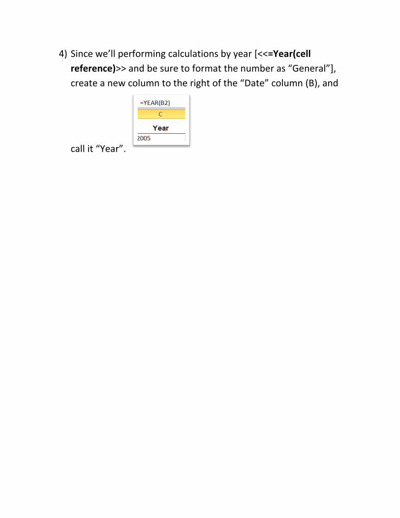
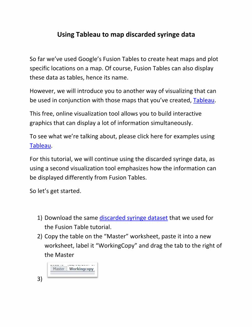
4) Since we’ll performing calculations by year [<<=Year(cell reference)>> and be sure to format the number as “General”], create a new column to the right of the “Date” column (B), and
call it “Year”.
McKied
Oval
McKied
Oval
Year”.
McKied
Oval
McKied
Oval

5) Create a pivot table in which you count the number of records in
the table using the ID number (SR#) in column A, place the “Year” column in the pivot table’s “Year” section, and place the “Ward” column in the “Row Label” section. As you will do with each new worksheet, be sure to drag the tab to the right of the preceding
McKied
Rectangle
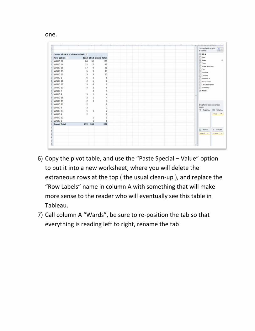
one.
6) Copy the pivot table, and use the “Paste Special – Value” option
to put it into a new worksheet, where you will delete the extraneous rows at the top ( the usual clean-up ), and replace the “Row Labels” name in column A with something that will make more sense to the reader who will eventually see this table in Tableau.
7) Call column A “Wards”, be sure to re-position the tab so that everything is reading left to right, rename the tab
McKied
Oval
McKied
Oval
McKied
Oval
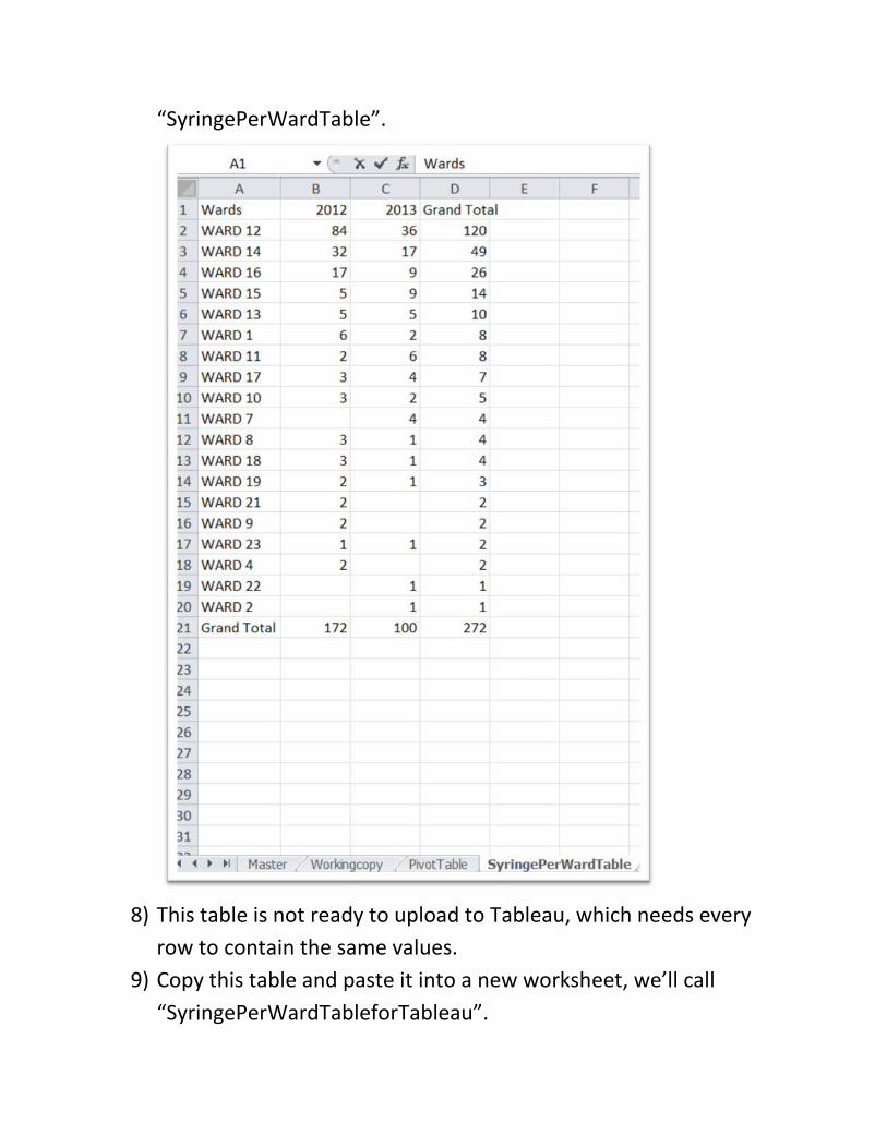
“SyringePerWardTable”.
8) This table is not ready to upload to Tableau, which needs every
row to contain the same values. 9) Copy this table and paste it into a new worksheet, we’ll call
“SyringePerWardTableforTableau”.
McKied
Oval
McKied
Oval
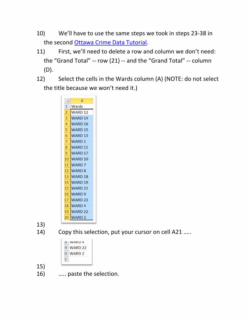
10) We’ll have to use the same steps we took in steps 23-38 in the second Ottawa Crime Data Tutorial.
11) First, we’ll need to delete a row and column we don’t need: the “Grand Total” -- row (21) -- and the “Grand Total” -- column (D).
12) Select the cells in the Wards column (A) (NOTE: do not select the title because we won’t need it.)
13) 14) Copy this selection, put your cursor on cell A21 …..
15) 16) ….. paste the selection.
McKied
Rectangle
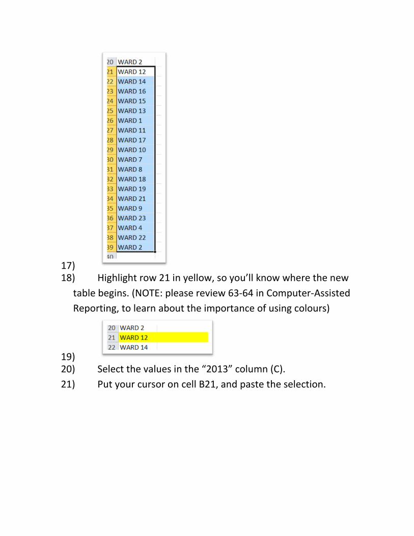
17) 18) Highlight row 21 in yellow, so you’ll know where the new
table begins. (NOTE: please review 63-64 in Computer-Assisted Reporting, to learn about the importance of using colours)
19) 20) Select the values in the “2013” column (C). 21) Put your cursor on cell B21, and paste the selection.
McKied
Rectangle
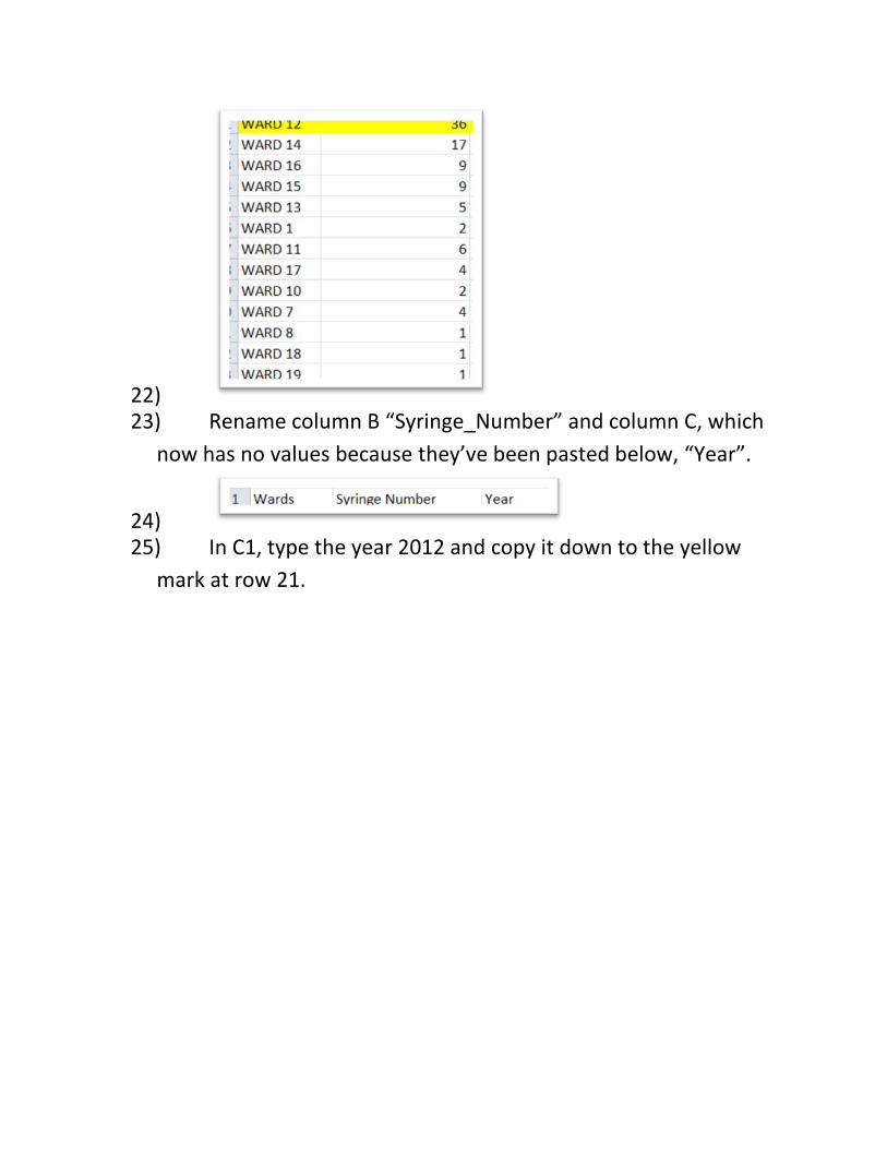
22) 23) Rename column B “Syringe_Number” and column C, which
now has no values because they’ve been pasted below, “Year”.
24) 25) In C1, type the year 2012 and copy it down to the yellow
mark at row 21.
McKied
Rectangle
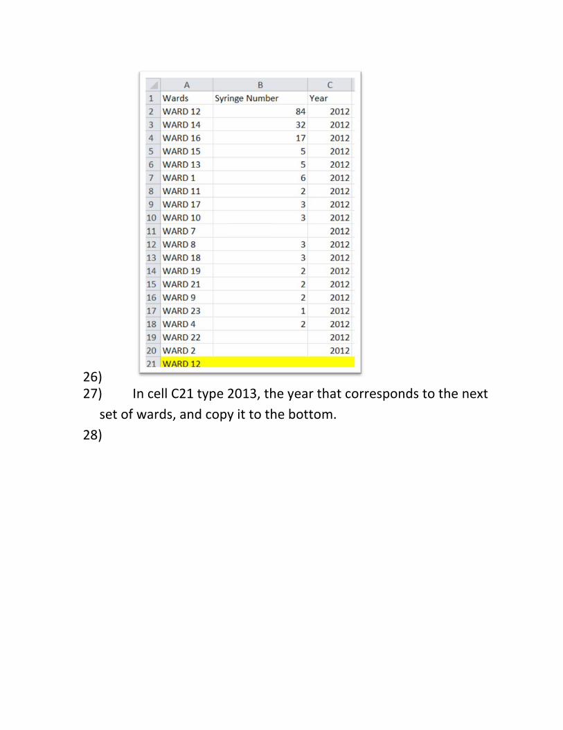
26) 27) In cell C21 type 2013, the year that corresponds to the next
set of wards, and copy it to the bottom. 28)
McKied
Rectangle
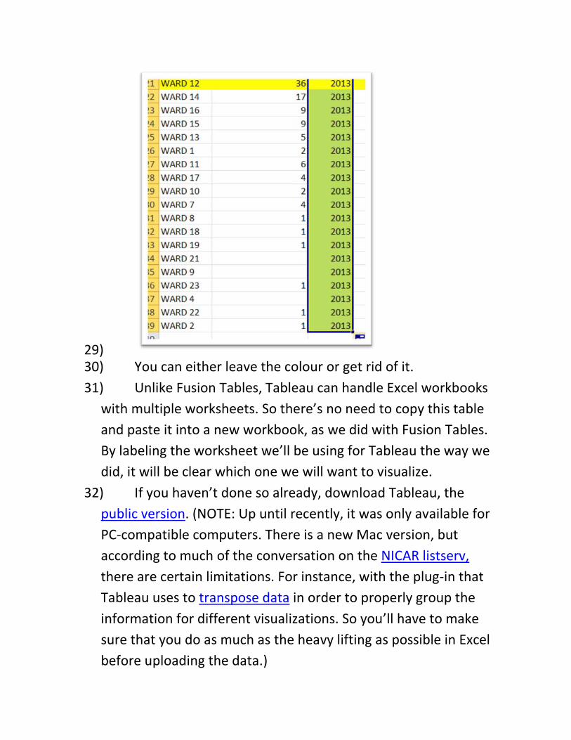
29) 30) You can either leave the colour or get rid of it. 31) Unlike Fusion Tables, Tableau can handle Excel workbooks
with multiple worksheets. So there’s no need to copy this table and paste it into a new workbook, as we did with Fusion Tables. By labeling the worksheet we’ll be using for Tableau the way we did, it will be clear which one we will want to visualize.
32) If you haven’t done so already, download Tableau, the public version. (NOTE: Up until recently, it was only available for PC-compatible computers. There is a new Mac version, but according to much of the conversation on the NICAR listserv, there are certain limitations. For instance, with the plug-in that Tableau uses to transpose data in order to properly group the information for different visualizations. So you’ll have to make sure that you do as much as the heavy lifting as possible in Excel before uploading the data.)
McKied
Rectangle
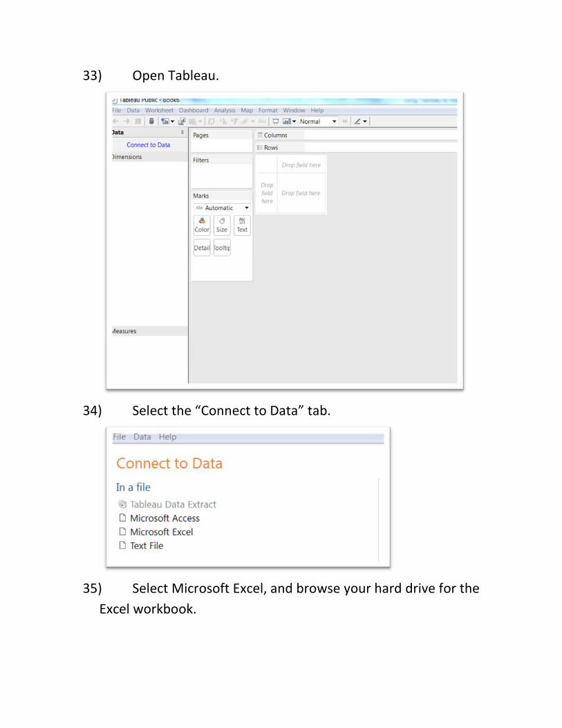
33) Open Tableau.
34) Select the “Connect to Data” tab.
35) Select Microsoft Excel, and browse your hard drive for the
Excel workbook.
McKied
Oval

36) Select the file, and be sure to highlight the proper worksheet, made easier because of the way we named it.
McKied
Rectangle
McKied
Oval

37) Pull the table into Tableau.
38) You’ll notice that the interface resembles Excel’s pivot table
( a key reason we’ve placed so much emphasis on learning pivot tables ). The “Measures” section is for columns with values” on which we will do math. Because it contains numbers, Tableau assumes we want to perform math on the values in the “Year” column. Not so. As in a pivot table, we only want to GROUP by year. So drag the “Year” tab into the Dimensions section, which is for text. (NOTE: If our table contained geographic coordinates such as country names, there would also be a globe icon in the

Dimensions section, allowing us to display those points on a map, which would then become part of the visualization package.)
39) As we would do in a pivot table, place the “Syringe Number” column in the table box for values, the bottom right. Or you can also place it in the “Text” icon under the “Marks section, which deals with dimensions and measures.
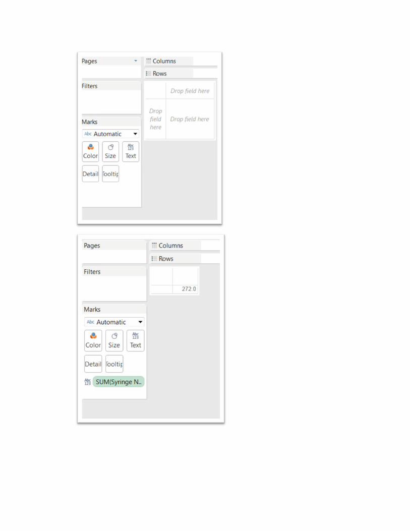
McKied
Oval
McKied
Oval
McKied
Oval
McKied
Oval
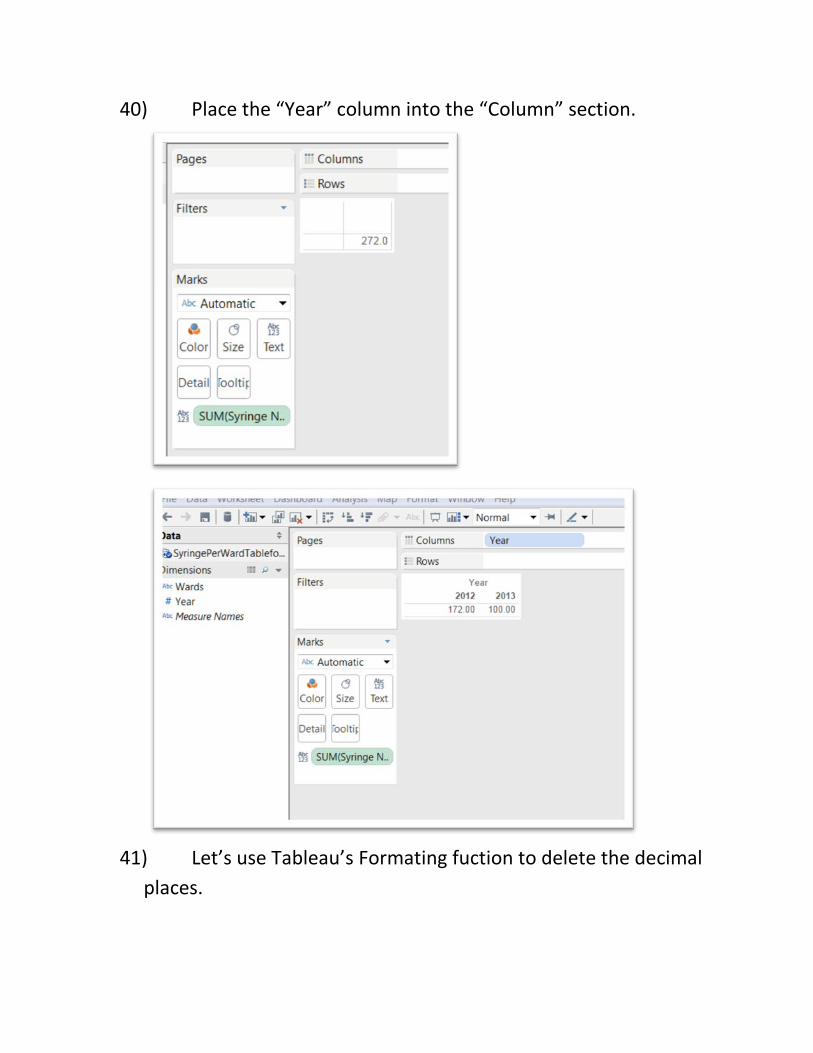
40) Place the “Year” column into the “Column” section.
41) Let’s use Tableau’s Formating fuction to delete the decimal
places.
McKied
Oval
McKied
Rectangle
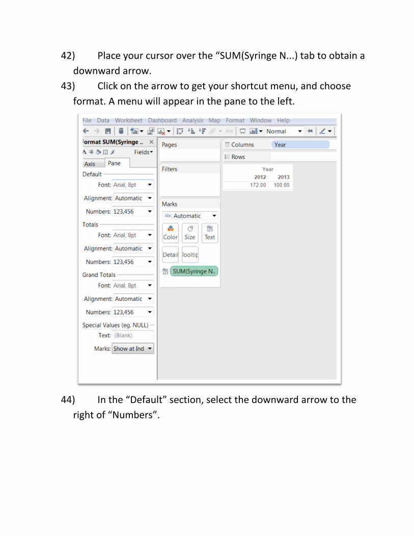
42) Place your cursor over the “SUM(Syringe N...) tab to obtain a downward arrow.
43) Click on the arrow to get your shortcut menu, and choose format. A menu will appear in the pane to the left.
44) In the “Default” section, select the downward arrow to the
right of “Numbers”.
McKied
Rectangle
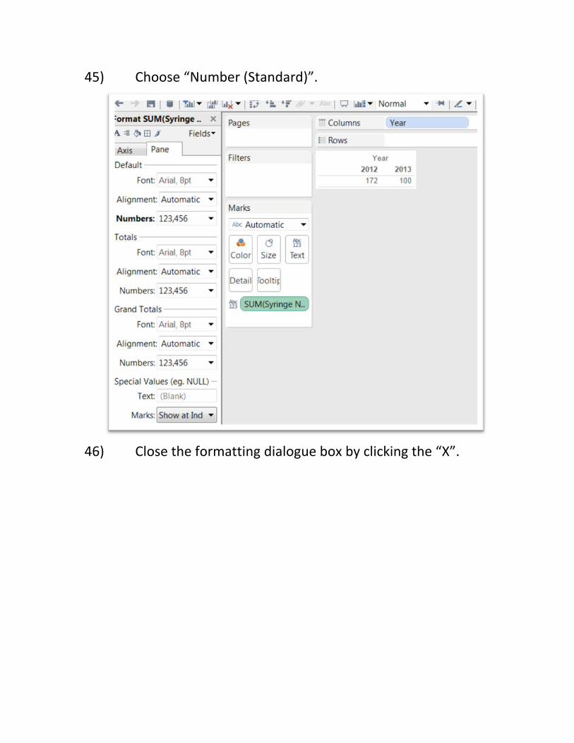
45) Choose “Number (Standard)”.
46) Close the formatting dialogue box by clicking the “X”.
McKied
Rectangle
McKied
Oval
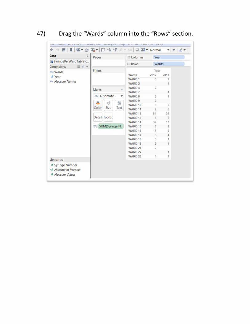
47) Drag the “Wards” column into the “Rows” section.
McKied
Rectangle
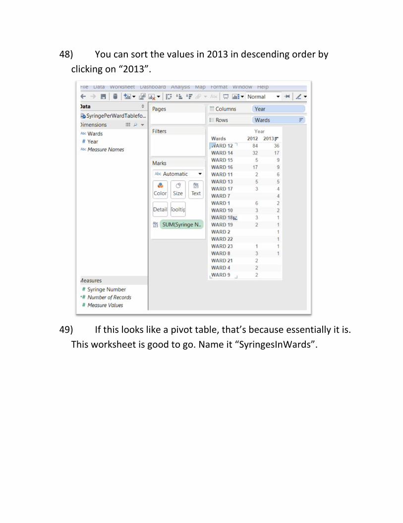
48) You can sort the values in 2013 in descending order by clicking on “2013”.
49) If this looks like a pivot table, that’s because essentially it is.
This worksheet is good to go. Name it “SyringesInWards”.
McKied
Oval
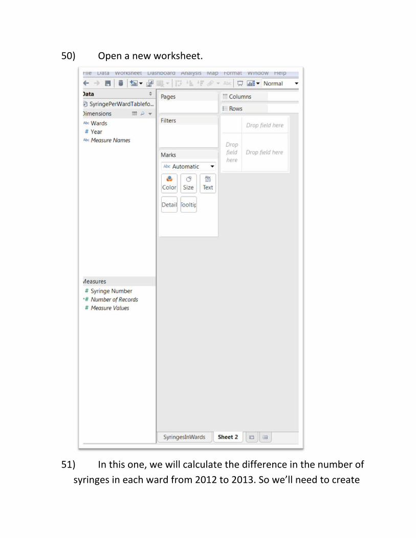
50) Open a new worksheet.
51) In this one, we will calculate the difference in the number of
syringes in each ward from 2012 to 2013. So we’ll need to create

the same table as we did in the “SyringesInWards” worksheet.
McKied
Oval
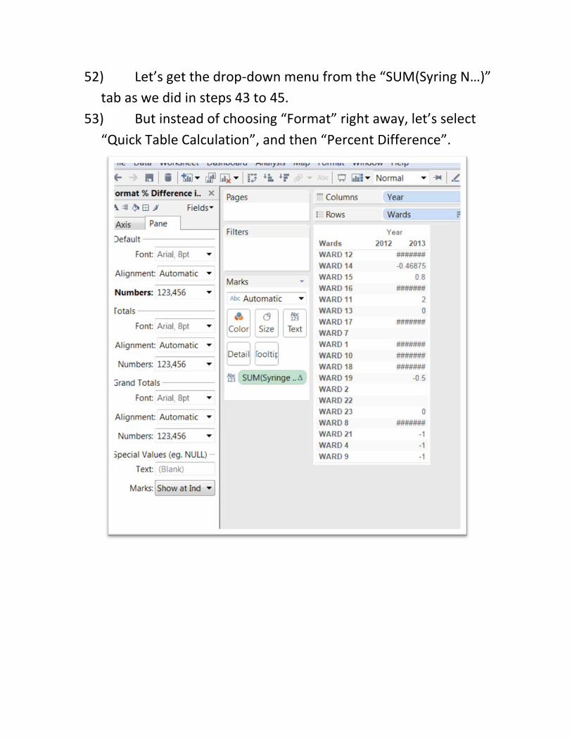
52) Let’s get the drop-down menu from the “SUM(Syring N…)” tab as we did in steps 43 to 45.
53) But instead of choosing “Format” right away, let’s select “Quick Table Calculation”, and then “Percent Difference”.
McKied
Oval
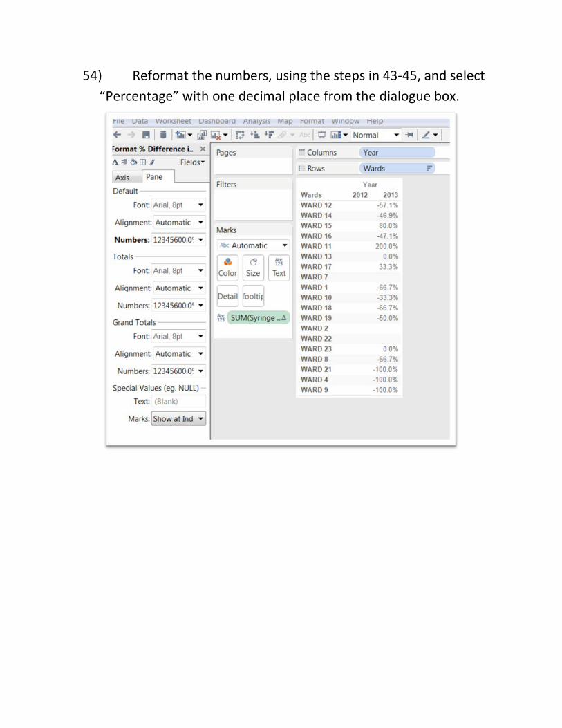
54) Reformat the numbers, using the steps in 43-45, and select “Percentage” with one decimal place from the dialogue box.
McKied
Rectangle
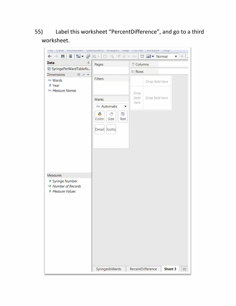
55) Label this worksheet “PercentDifference”, and go to a third worksheet.
McKied
Oval
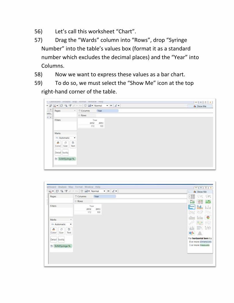
56) Let’s call this worksheet “Chart”. 57) Drag the “Wards” column into “Rows”, drop “Syringe
Number” into the table’s values box (format it as a standard number which excludes the decimal places) and the “Year” into Columns.
58) Now we want to express these values as a bar chart. 59) To do so, we must select the “Show Me” icon at the top
right-hand corner of the table.
McKied
Oval
McKied
Rectangle
60) Show Me allows us to display the information in a variety of ways, a Tableau strength.
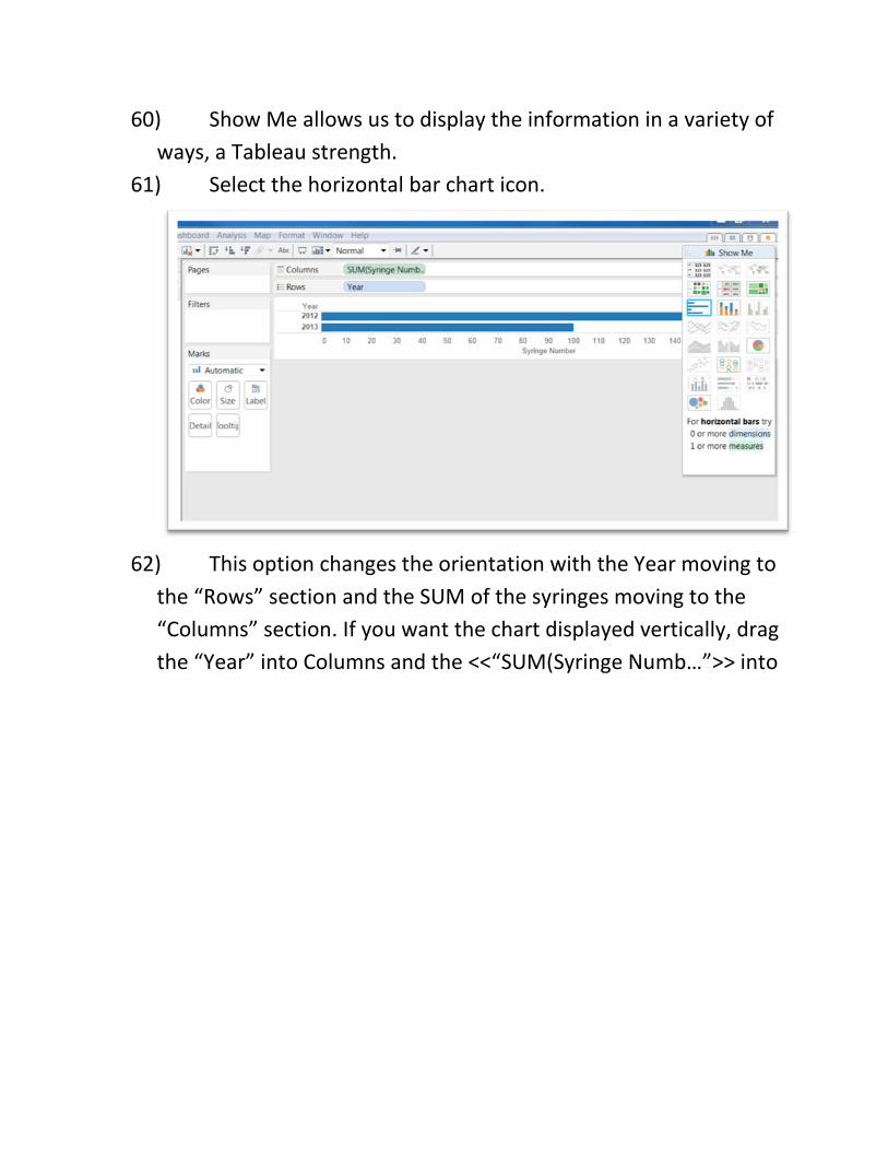
61) Select the horizontal bar chart icon.
62) This option changes the orientation with the Year moving to
the “Rows” section and the SUM of the syringes moving to the “Columns” section. If you want the chart displayed vertically, drag the “Year” into Columns and the <<“SUM(Syringe Numb…”>> into
McKied
Oval
McKied
Rectangle
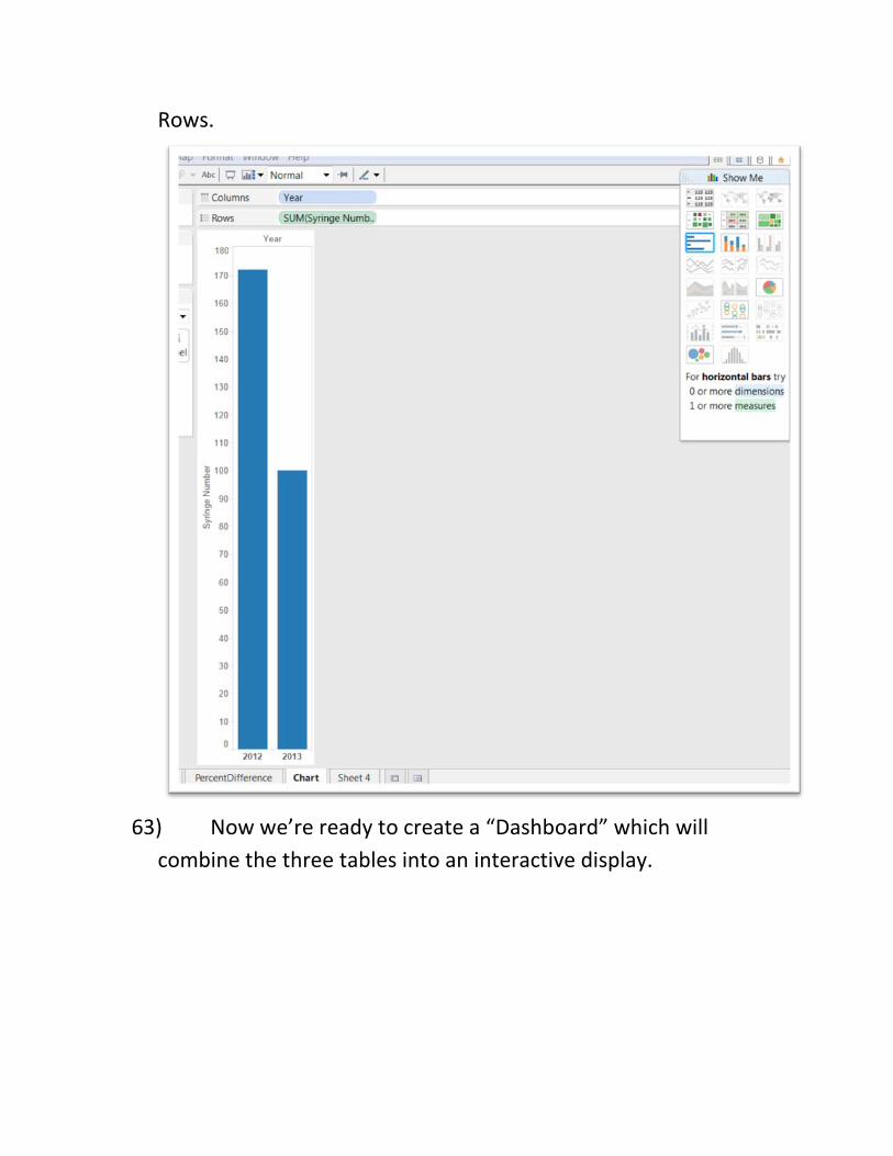
Rows.
63) Now we’re ready to create a “Dashboard” which will
combine the three tables into an interactive display.
McKied
Rectangle

64) Right click on the next worksheet and select the “New Dashboard” option.
65) Rename the Dashboard1 worksheet,
“SyringesPerWardDisplay”.
McKied
Oval
McKied
Rectangle
McKied
Oval
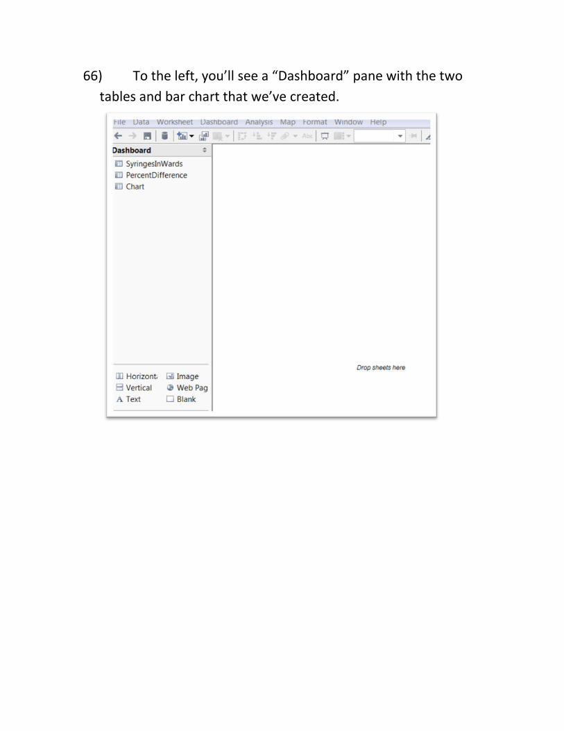
66) To the left, you’ll see a “Dashboard” pane with the two tables and bar chart that we’ve created.
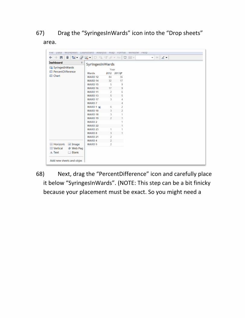
67) Drag the “SyringesInWards” icon into the “Drop sheets” area.
68) Next, drag the “PercentDifference” icon and carefully place
it below “SyringesInWards”. (NOTE: This step can be a bit finicky because your placement must be exact. So you might need a
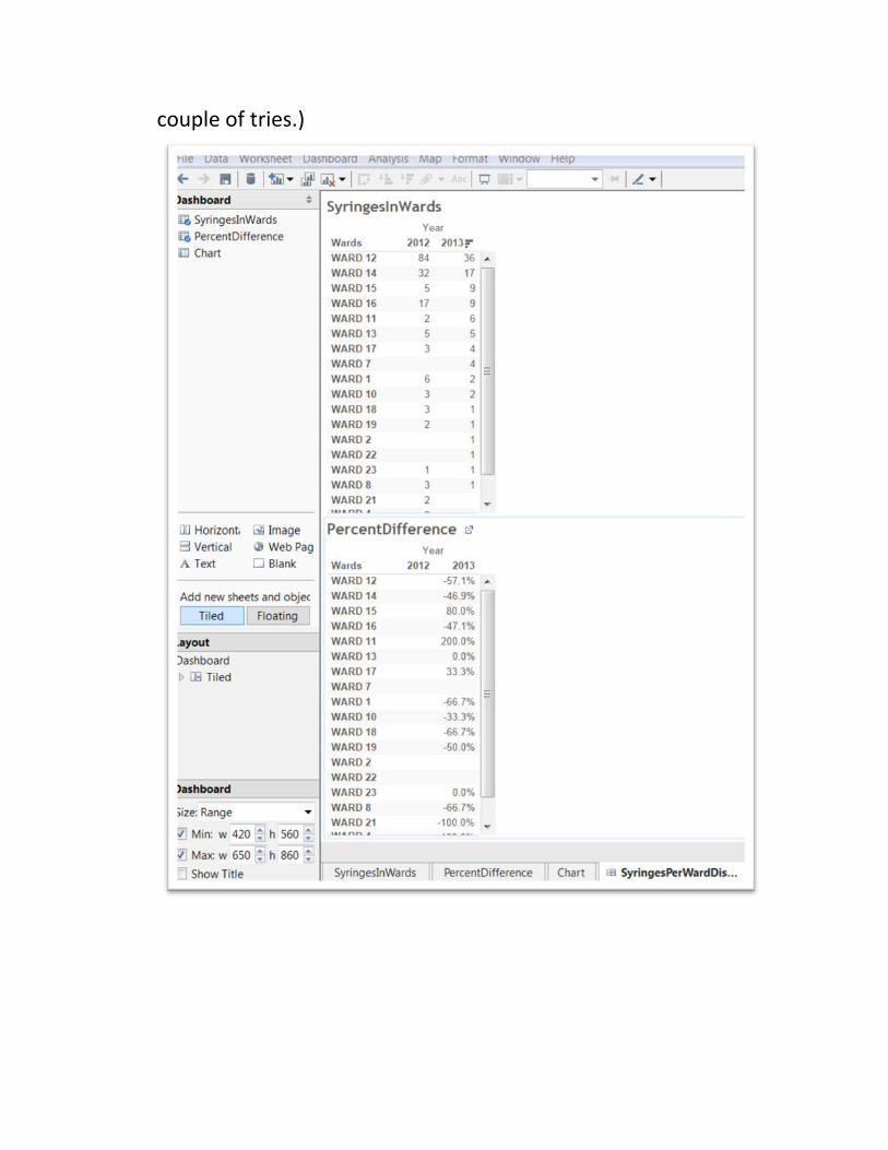
couple of tries.)
McKied
Oval
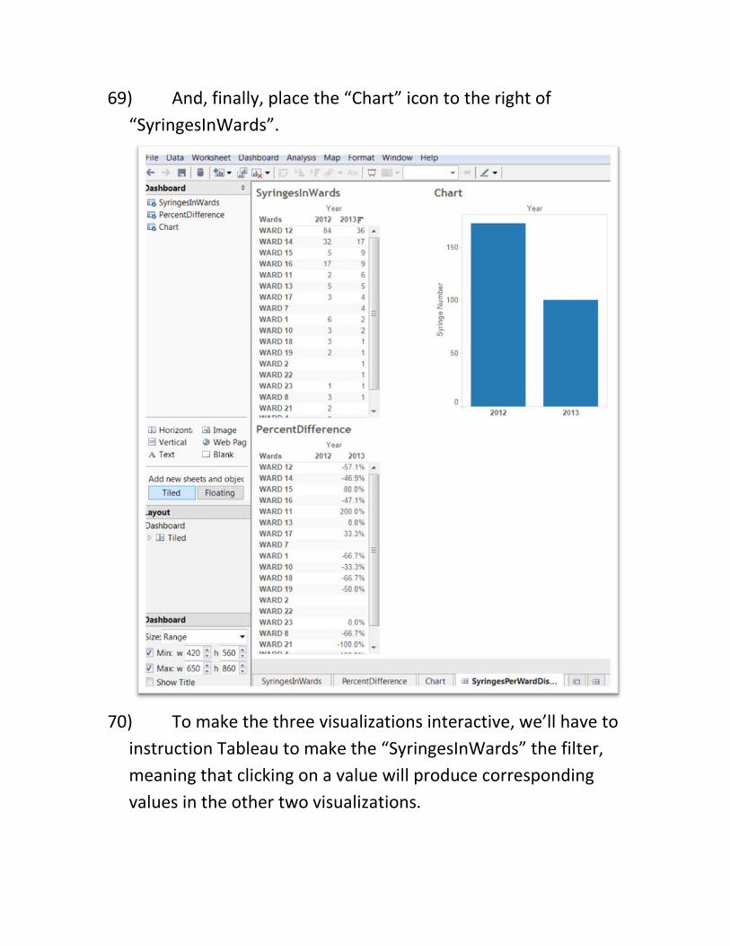
69) And, finally, place the “Chart” icon to the right of “SyringesInWards”.
70) To make the three visualizations interactive, we’ll have to
instruction Tableau to make the “SyringesInWards” the filter, meaning that clicking on a value will produce corresponding values in the other two visualizations.
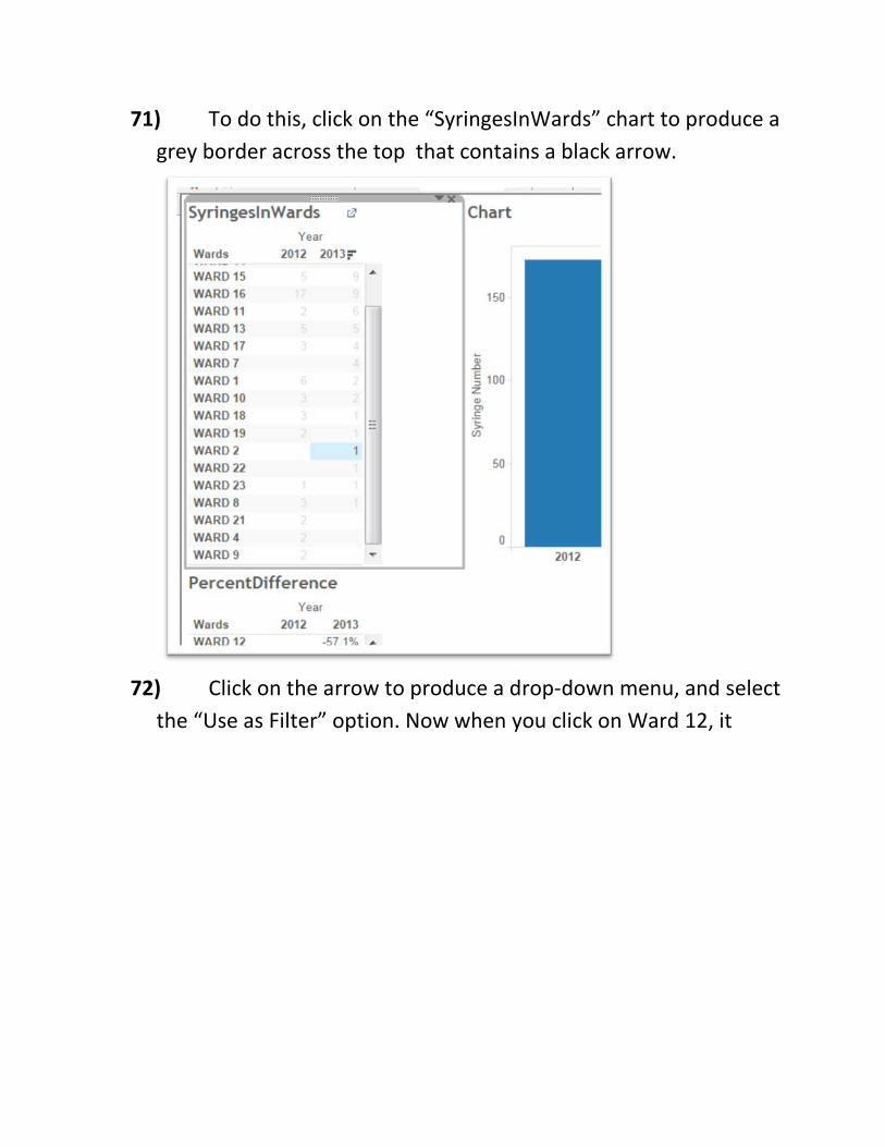
71) To do this, click on the “SyringesInWards” chart to produce a grey border across the top that contains a black arrow.
72) Click on the arrow to produce a drop-down menu, and select
the “Use as Filter” option. Now when you click on Ward 12, it

produces the corresponding values in the other two visualizations.
73) This is the chart we will upload to the Tableau server (as is
the case with Fusion Tables). 74) You can also change the proportions by selecting the
“Dashboard” option from the menu’s “Layout” section on the left. (NOTE: You can also do this directly in the embed code once you’ve placed it in HTML section of your blog post).
McKied
Rectangle
McKied
Oval

75) If you’re happy with the result (colour of chart, sizing, etc.), save the table by going to the “File” on the menu across the top….
76) …. And then “Save to the Web”, which will produce a “Login”
dialogue box.
McKied
Oval
McKied
Rectangle
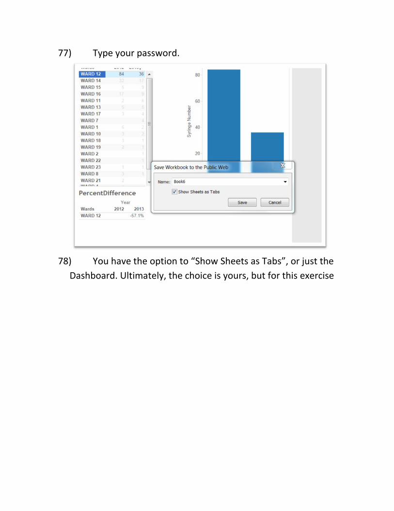
77) Type your password.
78) You have the option to “Show Sheets as Tabs”, or just the
Dashboard. Ultimately, the choice is yours, but for this exercise
McKied
Oval
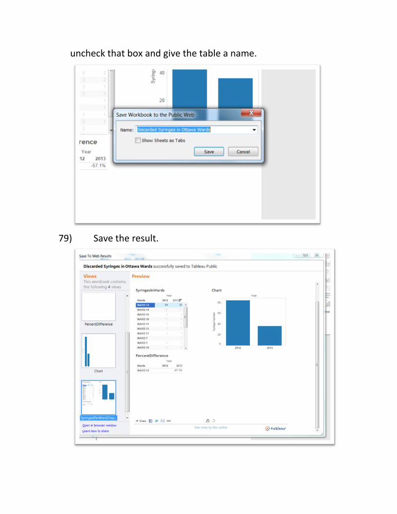
uncheck that box and give the table a name.
79) Save the result.
McKied
Oval
McKied
Oval
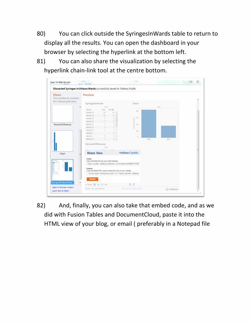
80) You can click outside the SyringesInWards table to return to display all the results. You can open the dashboard in your browser by selecting the hyperlink at the bottom left.
81) You can also share the visualization by selecting the hyperlink chain-link tool at the centre bottom.
82) And, finally, you can also take that embed code, and as we
did with Fusion Tables and DocumentCloud, paste it into the HTML view of your blog, or email ( preferably in a Notepad file
McKied
Rectangle
McKied
Oval
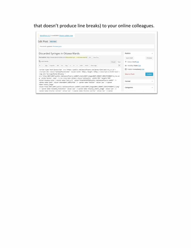
that doesn’t produce line breaks) to your online colleagues.
McKied
Oval
McKied
Oval
McKied
Oval
McKied
Oval
83)