Using Stata Graphics as a Method of Understanding and Presenting

Interaction Effects

Using Stata Graphics as a Method of Understanding and Presenting

Interaction Effects

Joanne M. Garrett, PhDUniversity of North Carolina at Chapel Hill

July 11, 2005

Problems with Understanding Interaction

• Interaction difficult concept to explain– not a single answer (point estimate)– linear combination of betas

• Often ignored because of difficulty

• Graph of interaction may be more intuitive for:– students learning the concept– presentations at professional meetings

Low Birth Weight Study*Low Birth Weight Study*

Variable Description Coding

low Low birth weigh 1 = ≤ 2500 gms

0 = >2500 gms

bwt Birth weight grams

smk Smoked during

pregnancy 1 = smoked

0 = did not smoke

race Mother’s race 1 = black

0 = white

age Mother’s age years

* “Loosely” adapted from data from Applied Logistic Regression, David W. Hosmer, Jr. and Stanley Lemeshow

Example 1: Low birth weight and interaction between smoking and race (1=black, 0=white)

Example 1: Low birth weight and interaction between smoking and race (1=black, 0=white)

Logistic regression model: Add smk by race interaction

Create interaction term and run logistic regression:

. gen smkxrace = smk * race

. logistic low smk race smkxrace

smkxraceracesmkeracesmklowDP

32101

1),|(

Example 1: Low birth weight and interaction between smoking and race (1=black, 0=white)

Example 1: Low birth weight and interaction between smoking and race (1=black, 0=white)

-------------------------------------------------- low | OR z P>|z| [95% CI]---------+---------------------------------------- smk | 5.76 4.14 0.000 2.51 13.19 race | 5.43 4.13 0.000 2.43 12.15smkxrace | .320 -2.08 0.038 .109 .936--------------------------------------------------

• Significant interaction: Relationship differs between smoking and low birth wt depending on mother’s race

• Question: How to interpret the interaction OR?

Example 1: Low birth weight and interaction between smoking and race (1=black, 0=white)

Example 1: Low birth weight and interaction between smoking and race (1=black, 0=white)

• Convert OR’s to beta coefficients and solve by categories of race: . logit

--------------------------------------------------

low | Coef. z P>|z| [95% CI]---------+---------------------------------------- smk | 1.751 4.14 0.000 0.921 2.580

race | 1.693 4.13 0.000 0.889 2.497smkxrace | -1.141 -2.08 0.038 -2.216 -0.066

_cons| -2.303 --------------------------------------------------

White: OR = e [β1 + β3(race)] = e [1.751 – 1.141(0)] = 5.76

Black: OR = e [β1 + β3(race)] = e [1.751 – 1.141(1)] = 1.84

Example 1: Low birth weight and interaction between smoking and race (1=black, 0=white)

Example 1: Low birth weight and interaction between smoking and race (1=black, 0=white)

White: . lincom smk + 0*smkxrace

---------------------------------------------- low | OR z P>|z| [95% CI] -----+---------------------------------------- (1) | 5.76 4.14 0.000 2.51 13.2 ----------------------------------------------

Black: . lincom smk + 1*smkxrace

---------------------------------------------- low | OR z P>|z| [95% CI] -----+---------------------------------------- (1) | 1.84 1.75 0.081 .928 3.65 ----------------------------------------------

Example 1: Low birth weight and interaction between smoking and race (1=black, 0=white)

Example 1: Low birth weight and interaction between smoking and race (1=black, 0=white)

Interpretation:

• Among whites, women who smoke have 5.8 times the odds of having a low birth wt baby

• Among blacks, there is no relationship between smoking and having a low birth wt baby (OR=1.8, but not statistically significant)

Example 1: Low birth weight and interaction between smoking and race (1=black, 0=white)

Example 1: Low birth weight and interaction between smoking and race (1=black, 0=white)

Misinterpretations:

• Black mothers have less “risk” for low birth wt babies compared to white mothers

• It’s okay for black mothers to smoke

Alternative:

• Solve the equation for values of smk and race

• Graph the individual probabilities (“predxcat”)

. predxcat low, xvar(race smk) graph bar

Example 1: Low birth weight and interaction between smoking and race (1=black, 0=white)

Example 1: Low birth weight and interaction between smoking and race (1=black, 0=white)

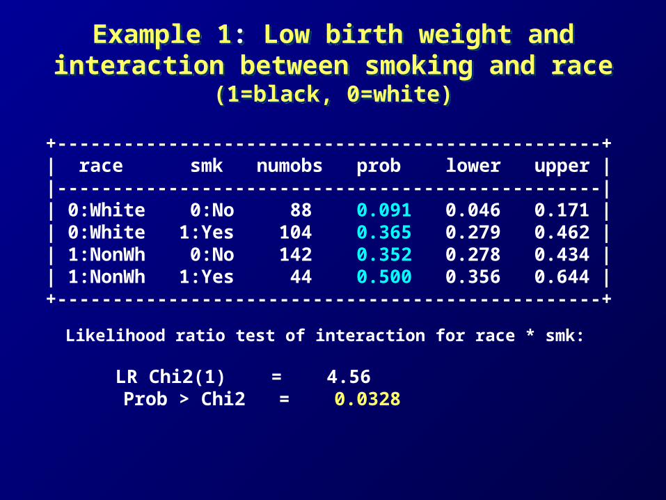
+-------------------------------------------------+| race smk numobs prob lower upper ||-------------------------------------------------|| 0:White 0:No 88 0.091 0.046 0.171 || 0:White 1:Yes 104 0.365 0.279 0.462 || 1:NonWh 0:No 142 0.352 0.278 0.434 || 1:NonWh 1:Yes 44 0.500 0.356 0.644 |+-------------------------------------------------+

Likelihood ratio test of interaction for race * smk:

LR Chi2(1) = 4.56 Prob > Chi2 = 0.0328

Example 1: Low birth weight and interaction between smoking and race (1=black, 0=white)

Example 1: Low birth weight and interaction between smoking and race (1=black, 0=white)

0

.1

.2

.3

.4

.5fo

r Lo

w B

irth

We

ight

0:White 1:Black

Una

djus

ted

Pro

babi

litie

s

Race

0:No 1:Yes

Smoked During Pregnancy

Example 2: Low birth weight and interaction between smoking and age (years)

Example 2: Low birth weight and interaction between smoking and age (years)

Logistic regression model: Add smk by age interaction

Create interaction term and run logistic regression:

. gen smkxage = smk * age

. logistic low smk age smkxage

smkxageagesmkeagesmklowDP

32101

1),|(

Example 2: Low birth weight and interaction between smoking and age (years)

Example 2: Low birth weight and interaction between smoking and age (years)

------------------------------------------------- low | OR z P>|z| [95% CI]---------+--------------------------------------- smk | 0.382 -0.90 0.367 .047 3.110 age | 0.920 -2.61 0.009 .865 0.980 smkxage | 1.076 1.97 0.049 1.001 1.157-------------------------------------------------

• Significant interaction: Relationship differs between smoking and low birth wt depending on mother’s age

• Question: How to interpret the interaction OR for a continuous interaction variable?

Example 2: Low birth weight and interaction between smoking and age (years)

Example 2: Low birth weight and interaction between smoking and age (years)

• Convert OR’s to beta coefficients and solve for selected values of age: . logit

------------------------------------------------- low | Coef. z P>|z| [95% CI] --------+----------------------------------------

smk | -.963 -0.90 0.367 -3.058 1.131 age | -.083 -2.61 0.009 -0.145 -0.021 smkxage | .073 1.97 0.049 0.001 0.146 _cons| .805 -------------------------------------------------

Age=15: OR = e [β1 + β3(age)] = e [–0.963 + 0.073(15)] = 1.14

Age=35: OR = e [β1 + β3(age)] = e [–0.963 + 0.073(35)] = 4.93

Example 2: Low birth weight and interaction between smoking and age (years)

Example 2: Low birth weight and interaction between smoking and age (years)

Age=15: . lincom smk + 15*smkxage

----------------------------------------------- low | OR z P>|z| [95% CI] -----+----------------------------------------- (1) | 1.14 0.32 0.751 .503 2.59 -----------------------------------------------

Age=35: . lincom smk + 35*smkxage

----------------------------------------------- low | OR z P>|z| [95% CI] -----+----------------------------------------- (1) | 4.93 2.59 0.010 1.47 16.5 -----------------------------------------------

Example 2: Low birth weight and interaction between smoking and age (years)

Example 2: Low birth weight and interaction between smoking and age (years)

Interpretation:

• Among 15 year olds, women who smoke have 1.1 times the odds of having a low birth wt baby

• Among 35 year olds, women who smoke have 4.9 times the odds of having a low birth wt baby

Example 2: Low birth weight and interaction between smoking and age (years)

Example 2: Low birth weight and interaction between smoking and age (years)

Misinterpretations:

• 15 year olds are not at risk for low birth wt babies

• It’s okay for 15 year olds to smoke

Alternative:

• Solve the equation and graph the probabilities for different levels of smoke and age (“predxcon”)

. predxcon low, xvar(age) from(15) to(35) inc(2) class(smk) graph

Example 2: Low birth weight and interaction between smoking and age (years)

Example 2: Low birth weight and interaction between smoking and age (years)

-> smk = 0 +---------------------------------+ | age pred_y lower upper | |---------------------------------| | 15 .392 .272 .527 | | 17 .353 .259 .461 | | 19 .317 .243 .400 | | (etc) ... ... ... | +---------------------------------+

-> smk = 1 +---------------------------------+ | age pred_y lower upper | |---------------------------------| | 15 .424 .285 .577 | | 17 .419 .303 .546 | | (etc) ... ... ... | +---------------------------------+

Likelihood ratio test for interaction of age * smk: LR Chi2(1) = 3.88 Prob > Chi2 = 0.05

Example 2: Low birth weight and interaction between smoking and age (years)

Example 2: Low birth weight and interaction between smoking and age (years)

p=0.05

.1

.2

.3

.4

.5

for

Low

Birt

h W

eig

ht

15 20 25 30 35Mother's Age

0:No 1:Yes

Smoked During Pregnancy

Pre

dict

ed

Pro

bab

ilitie

s

Example 3: Birth weight (grams) and interaction between smoking and raceExample 3: Birth weight (grams) and

interaction between smoking and race

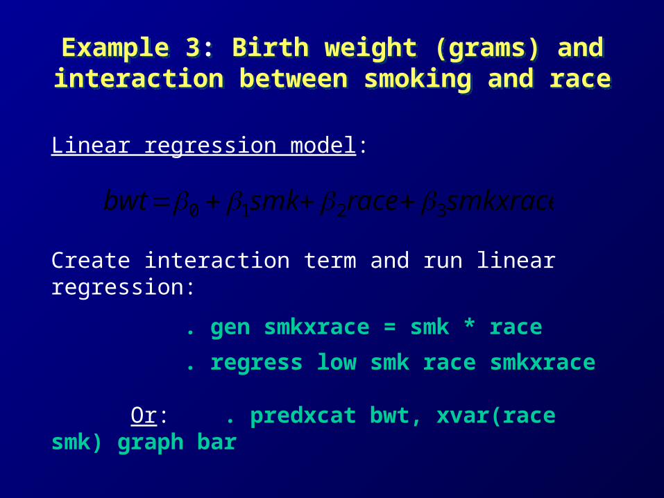
Linear regression model:

Create interaction term and run linear regression:

. gen smkxrace = smk * race

. regress low smk race smkxrace

Or: . predxcat bwt, xvar(race smk) graph bar

smkxraceracesmkbwt 3210

Example 3: Birth weight (grams) and interaction between smoking and raceExample 3: Birth weight (grams) and

interaction between smoking and race

p=0.006

0

1,000

2,000

3,000

4,000fo

r B

irth

We

ight

in G

ram

s

0:White 1:Black

Una

djus

ted

Me

ans

Race

0:No 1:YesSmoked During Pregnancy

Example 4: Birth weight (grams) and interaction between smoking and ageExample 4: Birth weight (grams) and interaction between smoking and age

Linear regression model:

Create interaction term and run linear regression:

. gen smkxage = smk * age

. regress low smk age smkxage

Or: . predxcon bwt, xvar(age) from(15) to(35) inc(2) class(smk) graph

smkxageagesmkbwt 3210

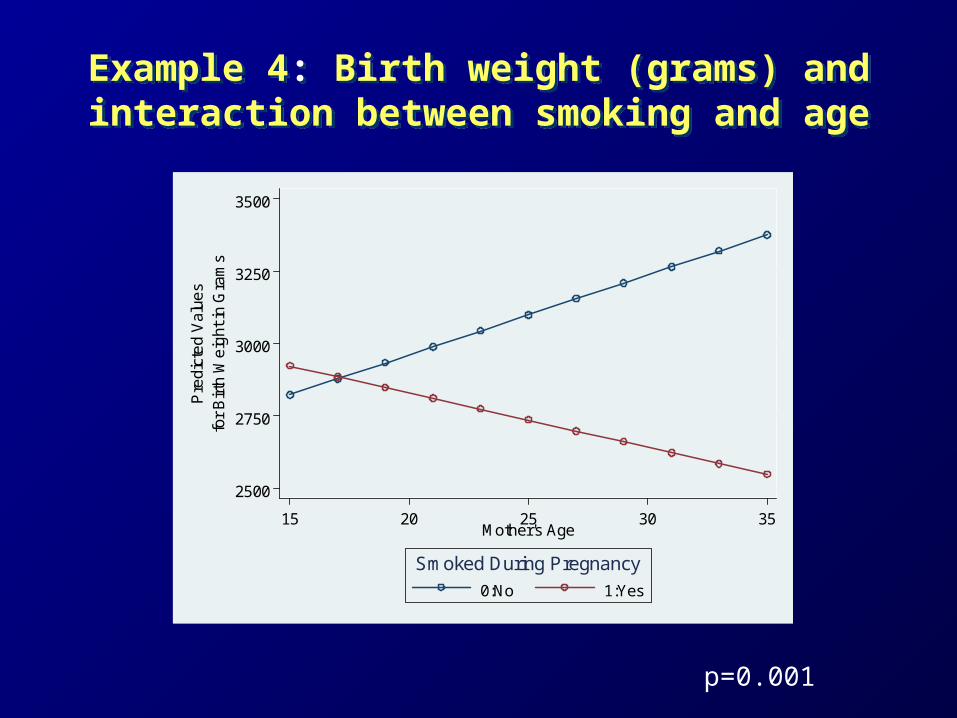
Example 4: Birth weight (grams) and interaction between smoking and ageExample 4: Birth weight (grams) and interaction between smoking and age

p=0.001

2500

2750

3000

3250

3500fo

r B

irth

We

ight

in G

ram

s

15 20 25 30 35Mother's Age

0:No 1:YesSmoked During Pregnancy

Pre

dict

ed

Val

ues

Example 5: Birth weight (grams) and interaction between smoking and age, age2, age3

Example 5: Birth weight (grams) and interaction between smoking and age, age2, age3

Linear regression model: add quadratic & cubic terms

Create interaction terms and run linear regression:

. gen age2 = age^2

. gen age3 = age^3

. gen smkxage = smk * age

. gen smkxage2 = smk * age2

. gen smkxage3 = smk * age3

. regress low smk age age2 age3 smkxage smkxage2 smkxage3

Or: . predxcon bwt, xvar(age) from(15) to(35) inc(2) class(smk) graph poly(3)

Example 5: Birth weight (grams) and interaction between smoking and age, age2, age3

Example 5: Birth weight (grams) and interaction between smoking and age, age2, age3

p=0.045

2500

2750

3000

3250

3500fo

r B

irth

We

ight

in G

ram

s

15 20 25 30 35Mother's Age (cubic)

0:No 1:YesSmoked During Pregnancy

Pre

dict

ed

Val

ues

Conclusions

• Interaction can be a difficult concept for people unfamiliar with the methodology

• Examining a graph of an interaction is an easier way to get an intuitive feel for the effect

• A useful technique for explaining interaction to students hearing it for the first time, before introducing mathematical models

• A simple way to present study results at meetings, even to a statistically savvy audience

. predxcat yvar, xvar(xvar1 xvar2)

yvar – dependent variable

continuous – defaults to linear regression binary (0,1) – defaults to logistic regression

xvar(xvar) – nominal variable for categories of estimated means or proportions

xvar(xvar1 xvar2) – categories of all combinations of xvar1 and xvar2; tests interaction

adjust(cov_list) – adjusts for any covariates

Calculating and Graphing Predicted Values: (when “X” is categorical)

graph – display graph (otherwise shows list of predicted values only)

bar – bar graph (instead of symbols – default)

model – for display purposes only; displays regression model

Some other options: level(#) cluster(cluster_id) savepred(ds_name)

Calculating and Graphing Predicted Values: (when “X” is categorical)

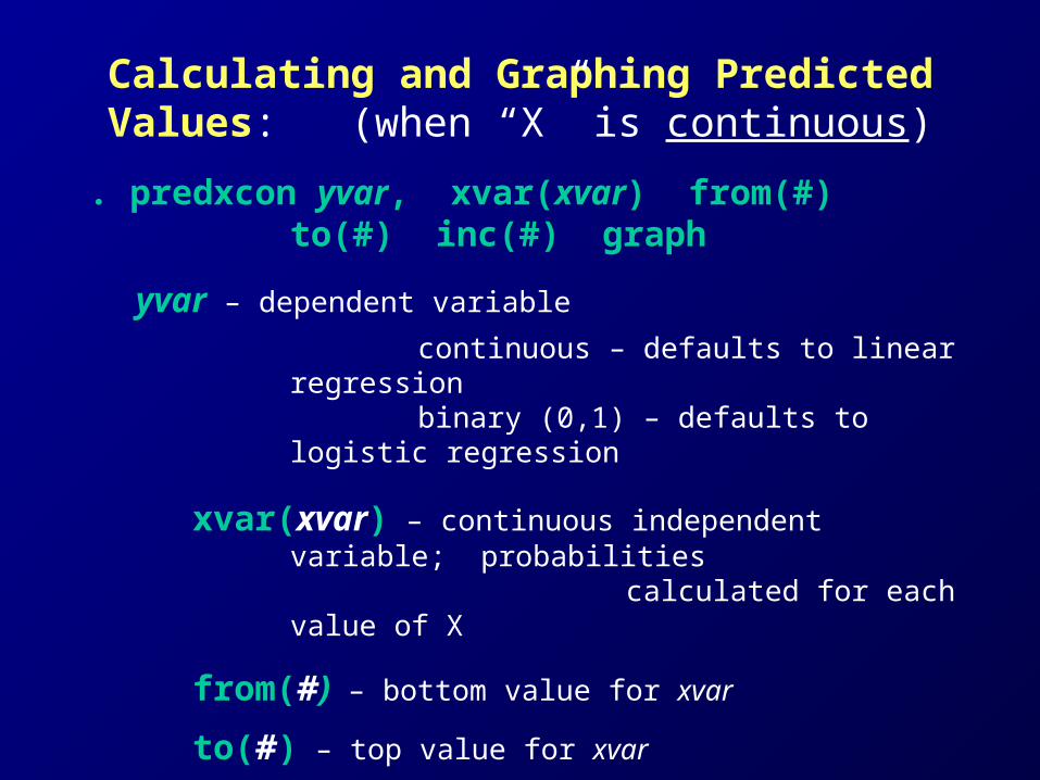
. predxcon yvar, xvar(xvar) from(#) to(#) inc(#) graph

yvar – dependent variable

continuous – defaults to linear regression binary (0,1) – defaults to logistic regression

xvar(xvar) – continuous independent variable; probabilities calculated for each value of X

from(#) – bottom value for xvar

to(#) – top value for xvar

inc(#) – increment desired between bottom and top values

adjust(cov_list) – adjusts for any covariates

Calculating and Graphing Predicted Values: (when “X” is continuous)

graph – display graph (otherwise shows list of predicted values only)

class(class_var) – adds an xvar by class_var interaction term

poly(2 or 3) – polynomial terms added: 2=squared

3=squared and cubic

model – for display purposes only; displays regression model

Some other options: level(#) cluster(cluster_id) nolist savepred(ds_name)

Calculating and Graphing Predicted Values: (when “X” is continuous)