Using SPSS for Multiple Regression

UDP 520 Lab 7Lin Lin

December 4th , 2007

Step 1 — Define Research Question

• What factors are associated with BMI?

• Predict BMI.

Step 2 — Conceptualizing Problem (Theory)

Individual Behaviors

BMI

EnvironmentIndividual Characteristics

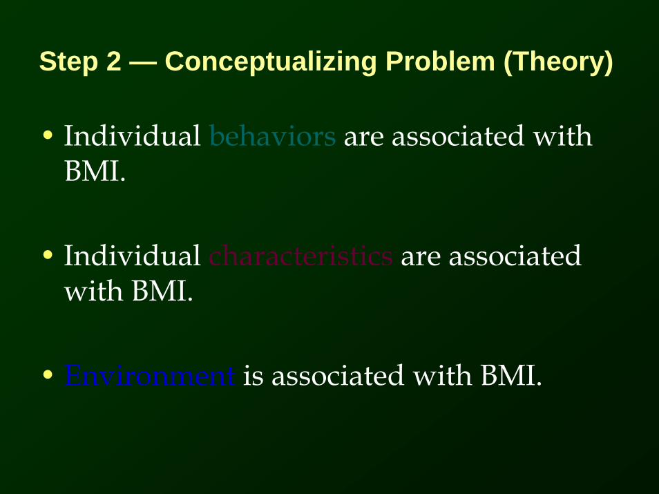
Step 2 — Conceptualizing Problem (Theory)

• Individual behaviors are associated with BMI.

• Individual characteristics are associated with BMI.

• Environment is associated with BMI.

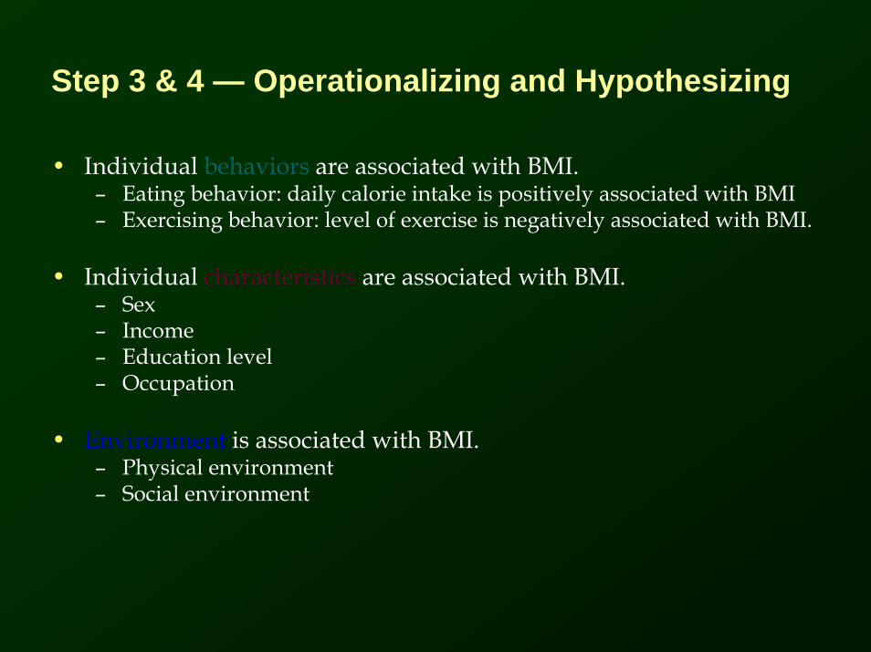
Step 3 & 4 — Operationalizing and Hypothesizing

• Individual behaviors are associated with BMI. – Eating behavior: daily calorie intake is positively associated with BMI– Exercising behavior: level of exercise is negatively associated with BMI.

• Individual characteristics are associated with BMI.– Sex– Income– Education level– Occupation

• Environment is associated with BMI.– Physical environment– Social environment

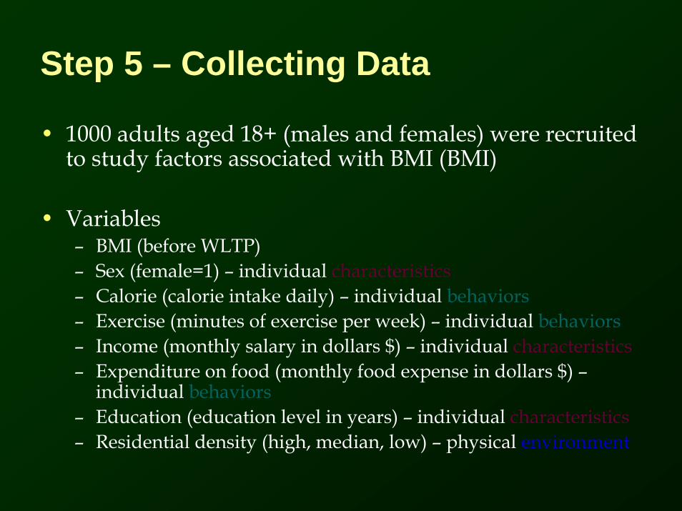
Step 5 – Collecting Data

• 1000 adults aged 18+ (males and females) were recruited to study factors associated with BMI (BMI)

• Variables– BMI (before WLTP)– Sex (female=1) – individual characteristics– Calorie (calorie intake daily) – individual behaviors– Exercise (minutes of exercise per week) – individual behaviors– Income (monthly salary in dollars $) – individual characteristics– Expenditure on food (monthly food expense in dollars $) –

individual behaviors– Education (education level in years) – individual characteristics– Residential density (high, median, low) – physical environment

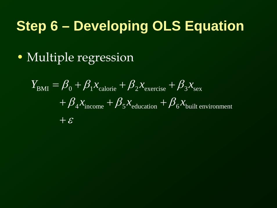
Step 6 – Developing OLS Equation

• Multiple regression

BMI 0 1 calorie 2 exercise 3 sex

4 income 5 education 6 built environment

Y x x xx x x

β β β ββ β βε

= + + ++ + +

+

OLS Equation for SPSS

• Multiple regression Model 1

BMI 0 1 calorie 2 exercise

4 income 5 education

Y x xx x

β β ββ βε

= + +

+ +

+

Using SPSS for Multiple Regression

SPSS Output Tables

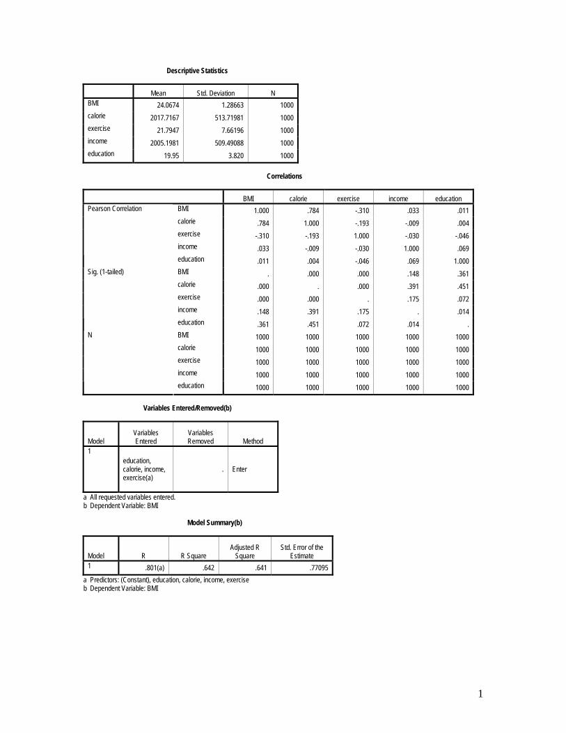
Descriptive Statistics

Mean Std. Deviation N BMI 24.0674 1.28663 1000 calorie 2017.7167 513.71981 1000 exercise 21.7947 7.66196 1000 income 2005.1981 509.49088 1000 education 19.95 3.820 1000

Correlations

BMI calorie exercise income education BMI 1.000 .784 -.310 .033 .011 calorie .784 1.000 -.193 -.009 .004 exercise -.310 -.193 1.000 -.030 -.046 income .033 -.009 -.030 1.000 .069

Pearson Correlation

education .011 .004 -.046 .069 1.000 BMI . .000 .000 .148 .361 calorie .000 . .000 .391 .451 exercise .000 .000 . .175 .072 income .148 .391 .175 . .014

Sig. (1-tailed)

education .361 .451 .072 .014 . BMI 1000 1000 1000 1000 1000 calorie 1000 1000 1000 1000 1000 exercise 1000 1000 1000 1000 1000 income 1000 1000 1000 1000 1000

N

education 1000 1000 1000 1000 1000 Variables Entered/Removed(b)

Model Variables Entered

Variables Removed Method

1 education, calorie, income, exercise(a)

. Enter

a All requested variables entered. b Dependent Variable: BMI Model Summary(b)

Model R R Square Adjusted R

Square Std. Error of the

Estimate 1 .801(a) .642 .641 .77095

a Predictors: (Constant), education, calorie, income, exercise b Dependent Variable: BMI

1

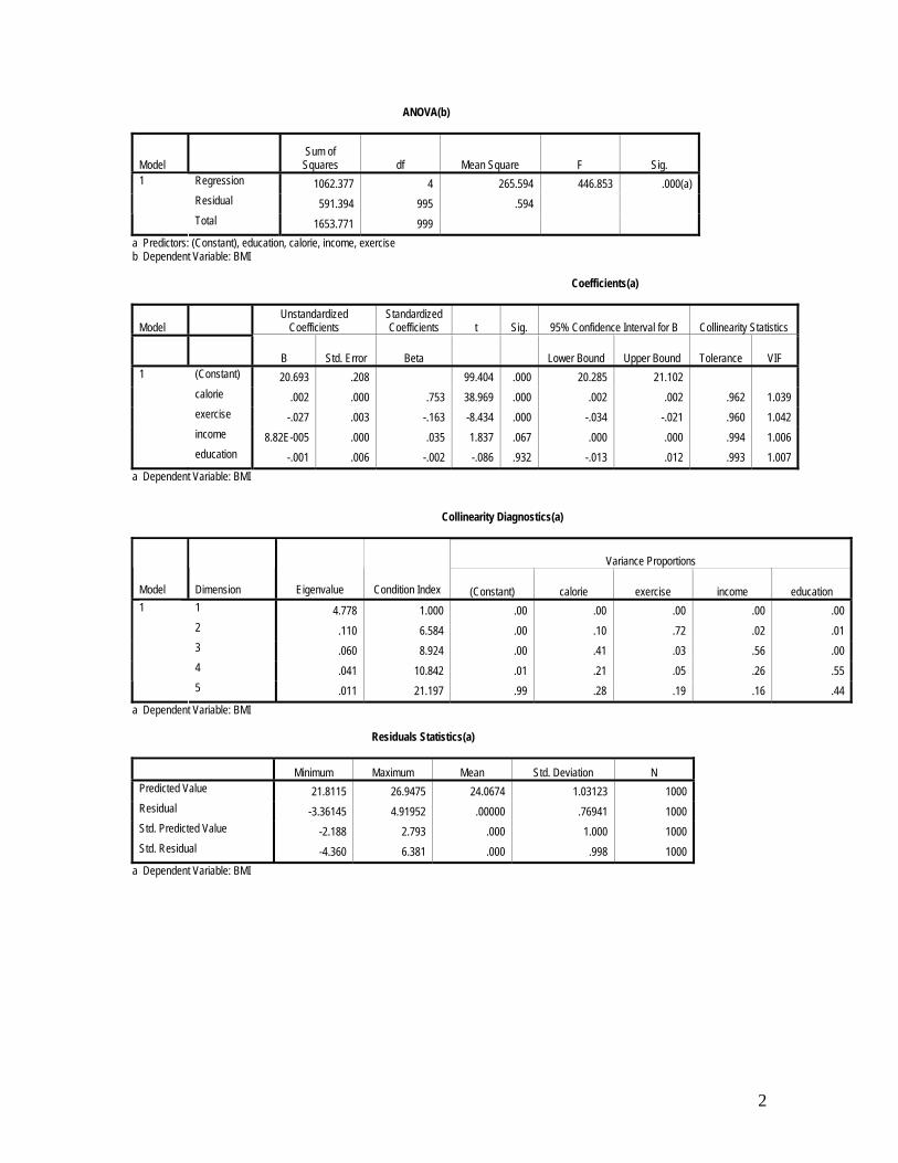
ANOVA(b)

Model Sum of

Squares df Mean Square F Sig. Regression 1062.377 4 265.594 446.853 .000(a) Residual 591.394 995 .594

1

Total 1653.771 999 a Predictors: (Constant), education, calorie, income, exercise b Dependent Variable: BMI Coefficients(a)

Model Unstandardized

Coefficients Standardized Coefficients t Sig. 95% Confidence Interval for B Collinearity Statistics

B Std. Error Beta Lower Bound Upper Bound Tolerance VIF 1 (Constant) 20.693 .208 99.404 .000 20.285 21.102 calorie .002 .000 .753 38.969 .000 .002 .002 .962 1.039 exercise -.027 .003 -.163 -8.434 .000 -.034 -.021 .960 1.042 income 8.82E-005 .000 .035 1.837 .067 .000 .000 .994 1.006 education -.001 .006 -.002 -.086 .932 -.013 .012 .993 1.007

a Dependent Variable: BMI Collinearity Diagnostics(a)

Variance Proportions

Model Dimension Eigenvalue Condition Index (Constant) calorie exercise income education 1 4.778 1.000 .00 .00 .00 .00 .00 2 .110 6.584 .00 .10 .72 .02 .01 3 .060 8.924 .00 .41 .03 .56 .00 4 .041 10.842 .01 .21 .05 .26 .55

1

5 .011 21.197 .99 .28 .19 .16 .44 a Dependent Variable: BMI Residuals Statistics(a)

Minimum Maximum Mean Std. Deviation N Predicted Value 21.8115 26.9475 24.0674 1.03123 1000 Residual -3.36145 4.91952 .00000 .76941 1000 Std. Predicted Value -2.188 2.793 .000 1.000 1000 Std. Residual -4.360 6.381 .000 .998 1000

a Dependent Variable: BMI

2

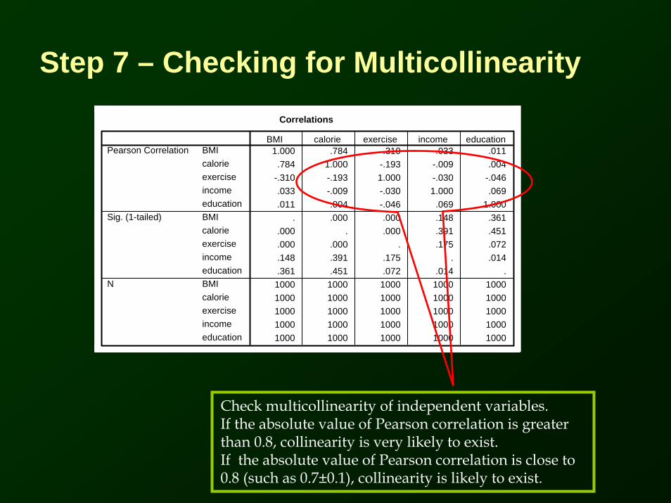
Step 7 – Checking for MulticollinearityCorrelations

1.000 .784 -.310 .033 .011.784 1.000 -.193 -.009 .004

-.310 -.193 1.000 -.030 -.046.033 -.009 -.030 1.000 .069.011 .004 -.046 .069 1.000

. .000 .000 .148 .361.000 . .000 .391 .451.000 .000 . .175 .072.148 .391 .175 . .014.361 .451 .072 .014 .

1000 1000 1000 1000 10001000 1000 1000 1000 10001000 1000 1000 1000 10001000 1000 1000 1000 10001000 1000 1000 1000 1000

BMIcalorieexerciseincomeeducationBMIcalorieexerciseincomeeducationBMIcalorieexerciseincomeeducation

Pearson Correlation

Sig. (1-tailed)

N

BMI calorie exercise income education

Check multicollinearity of independent variables.If the absolute value of Pearson correlation is greater than 0.8, collinearity is very likely to exist. If the absolute value of Pearson correlation is close to 0.8 (such as 0.7±0.1), collinearity is likely to exist.

Step 7 – Checking for Multicollinearity (cont.)

Collinearity Diagnosticsa

4.778 1.000 .00 .00 .00 .00 .00.110 6.584 .00 .10 .72 .02 .01.060 8.924 .00 .41 .03 .56 .00.041 10.842 .01 .21 .05 .26 .55.011 21.197 .99 .28 .19 .16 .44

Dimension12345

Model1

EigenvalueCondition

Index (Constant) calorie exercise income educationVariance Proportions

Dependent Variable: BMIa.

A condition index greater than 15 indicates a possible problem

An index greater than 30 suggests a serious problem with collinearity.

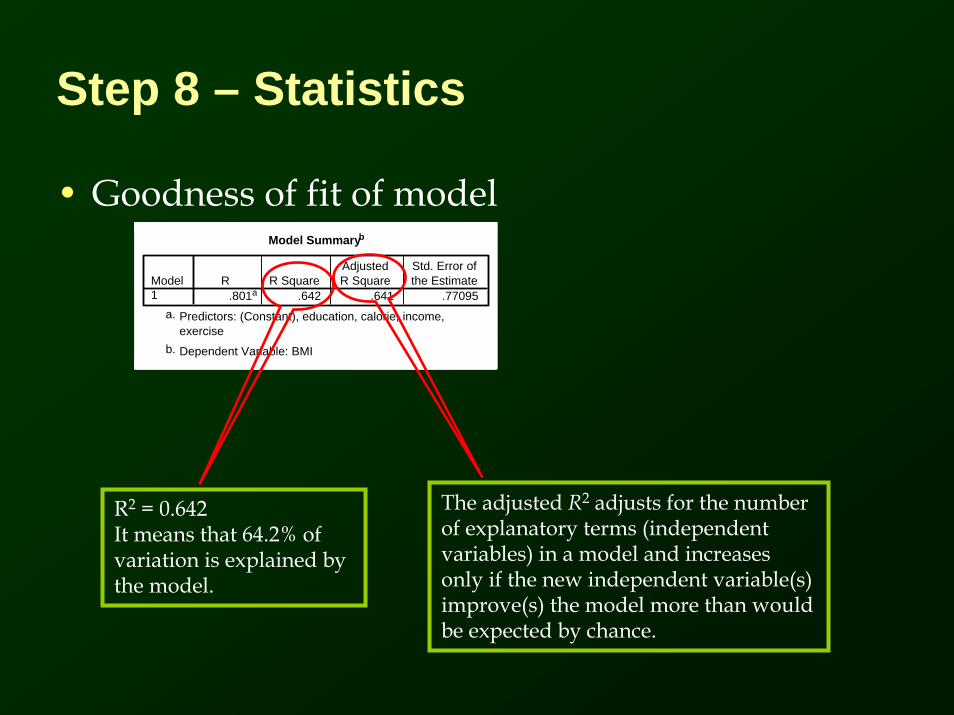
Step 8 – Statistics

• Goodness of fit of modelModel Summaryb

.801a .642 .641 .77095Model1

R R SquareAdjustedR Square

Std. Error ofthe Estimate

Predictors: (Constant), education, calorie, income,exercise

a.

Dependent Variable: BMIb.

R2 = 0.642 It means that 64.2% of variation is explained by the model.

The adjusted R2 adjusts for the number of explanatory terms (independent variables) in a model and increases only if the new independent variable(s) improve(s) the model more than would be expected by chance.

Step 8 – Statistics (cont.)

• Coefficient of each independent variable

Coefficientsa

20.693 .208 99.404 .000 20.285 21.102.002 .000 .753 38.969 .000 .002 .002 .962 1.039

-.027 .003 -.163 -8.434 .000 -.034 -.021 .960 1.0428.82E-005 .000 .035 1.837 .067 .000 .000 .994 1.006

-.001 .006 -.002 -.086 .932 -.013 .012 .993 1.007

(Constant)calorieexerciseincomeeducation

Model1

B Std. Error

UnstandardizedCoefficients

Beta

StandardizedCoefficients

t Sig. Lower Bound Upper Bound95% Confidence Interval for B

Tolerance VIFCollinearity Statistics

Dependent Variable: BMIa.

Unstandardizedcoefficients used in the prediction and interpretation

standardized coefficients used for comparing the effects of independent variables

Compared Sig. with alpha 0.05.

If Sig. <0.05 the coefficient is statistically significant from zero.

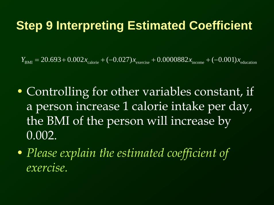
Step 9 Interpreting Estimated Coefficient

• Controlling for other variables constant, if a person increase 1 calorie intake per day, the BMI of the person will increase by 0.002.

• Please explain the estimated coefficient of exercise.

BMI calorie exercise income education20.693 0.002 ( 0.027) 0.0000882 ( 0.001)Y x x x x= + + − + + −

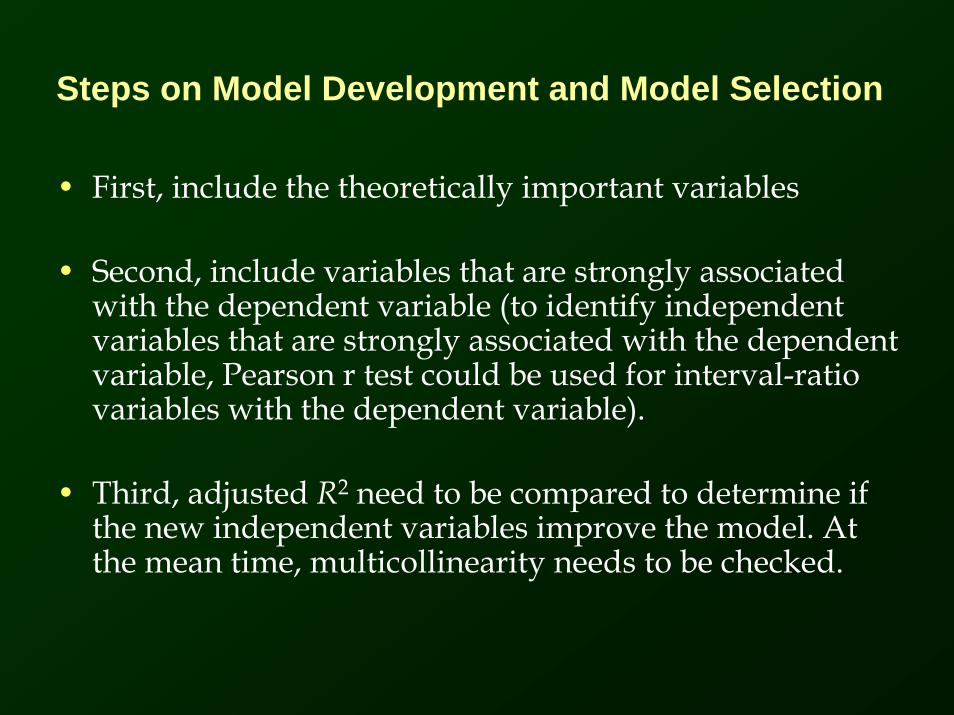
Steps on Model Development and Model Selection

• First, include the theoretically important variables

• Second, include variables that are strongly associated with the dependent variable (to identify independent variables that are strongly associated with the dependent variable, Pearson r test could be used for interval-ratio variables with the dependent variable).

• Third, adjusted R2 need to be compared to determine if the new independent variables improve the model. At the mean time, multicollinearity needs to be checked.

Notes on Regression Model

• It is VERY important to have theory before starting developing any regression model.

• If the theory tells you certain variables are too important to exclude from the model, you should include in the model even though their estimated coefficients are not significant. (Of course, it is more conservative way to develop regression model.)

BMI data

http://courses.washington.edu/urbdp520/UDP520/BMI.sav

For exercise, you can develop your own conceptual frameworks (theories), create different OLS models, and examine different independent variables.