Norwegian University of Science and Technology

TTK4550 – Specialization Project

Using Solar Panels as Sun Sensors onNTNU Test Satellite

Author:

Martin Nygren

Supervisor:

Prof. Jan Tommy Gravdahl

December 22, 2012

Abstract

The NUTS (NTNU Test Satellite) is a satellite being built as a student CubeSat project. The project

started in September 2010 as a part of the Norwegian student satellite program run by NAROM (Nor-

wegian Centre for Space-related Education). The NUTS project goals are to design, manufacture and

launch a double CubeSat by 2014.

Using solar panels on 5 of 6 sides of the NUTS CubeSat, we have a lot of attitude determinating informa-

tion readily available during much of the periodical orbit. Using three or more solar panels in combination

can trigonometrically produce a sun vector. However, treating all inbound sunlight as direct light from

the sun leaves the result vulnerable to disturbances like the Earth albedo effect (reflected sunlight from

the Earth), which is hard to model and computationally expensive to simulate. Not compensating for

this effect can corrupt or introduce large offsets in computed sun vectors.

Treating the output current from the solar panels as an angle of 3D inbound light towards the 2D plane

of the panel can produce a set of independent mathematical conical shells. Given the cubic shape of

the satellite, these independent conical shells can iteratively be combined into sets of two and two or-

thogonal conical shells which will produce intersection curves with eachother if the angle of aperture is

large enough. Even though the panels are physically spaced apart, it can be shown that without loss of

generality, these conical shells can be translated along their respective axis of the satellite BODY frame to

have overlapping origins, which we can use to map the convergences of the parabolic intersection curves

into two possible inbound sun vectors for each pair of solar panels. Knowing that opposing panels can’t

be combined to yield valid information, our 5 sides of panels can be combined into 8 different pairs from

which we can interpret information.

At the time of writing, MATLAB code to display computed sun vectors from conical shell intersections

produced by sets of panels in real time has been made and physical experiments are about to commence.

Algorithms to compare and evaluate the produced cluster of vectors to extract desired information and

suppress disturbance are in the making. Making use of instantaneous and tracked individual vectorial

attitudes as well as their rates of change seems promising, but special attention needs to be paid to the

Earth albedo effect in attempt to identify and suppress this disturbance.

Contents

Abstract . . . . . . . . . . . . . . . . . . . . . . . . . . . . . . . . . . . . . . . . . . . . . . . . . i

Table of Contents . . . . . . . . . . . . . . . . . . . . . . . . . . . . . . . . . . . . . . . . . . . . ii

List of Figures . . . . . . . . . . . . . . . . . . . . . . . . . . . . . . . . . . . . . . . . . . . . . iii

1 Introduction 1

2 Context 2

2.1 NUTS - NTNU Test Satellite . . . . . . . . . . . . . . . . . . . . . . . . . . . . . . . . . . 2

2.2 The components of the satellite . . . . . . . . . . . . . . . . . . . . . . . . . . . . . . . . . 2

2.2.1 Backplane . . . . . . . . . . . . . . . . . . . . . . . . . . . . . . . . . . . . . . . . . 3

2.2.2 Electrical Power System . . . . . . . . . . . . . . . . . . . . . . . . . . . . . . . . . 3

2.2.3 Onboard Computer . . . . . . . . . . . . . . . . . . . . . . . . . . . . . . . . . . . 4

2.2.4 Attitude Determination and Control System . . . . . . . . . . . . . . . . . . . . . . 4

2.2.5 Backplane sensors . . . . . . . . . . . . . . . . . . . . . . . . . . . . . . . . . . . . 4

2.2.6 Radio . . . . . . . . . . . . . . . . . . . . . . . . . . . . . . . . . . . . . . . . . . . 4

2.2.7 Payload . . . . . . . . . . . . . . . . . . . . . . . . . . . . . . . . . . . . . . . . . . 4

2.3 Assignment . . . . . . . . . . . . . . . . . . . . . . . . . . . . . . . . . . . . . . . . . . . . 5

2.3.1 Previous work on the ADCS . . . . . . . . . . . . . . . . . . . . . . . . . . . . . . 5

2.3.2 This report . . . . . . . . . . . . . . . . . . . . . . . . . . . . . . . . . . . . . . . . 5

3 Preliminaries 6

3.1 Attitude terminology . . . . . . . . . . . . . . . . . . . . . . . . . . . . . . . . . . . . . . . 6

3.2 Attitude representations . . . . . . . . . . . . . . . . . . . . . . . . . . . . . . . . . . . . . 6

3.2.1 Euler angles . . . . . . . . . . . . . . . . . . . . . . . . . . . . . . . . . . . . . . . . 7

3.3 Reference frames . . . . . . . . . . . . . . . . . . . . . . . . . . . . . . . . . . . . . . . . . 8

3.3.1 Earth Center Inertial (ECI) . . . . . . . . . . . . . . . . . . . . . . . . . . . . . . . 8

3.3.2 Earth Center Earth Fixed (ECEF) . . . . . . . . . . . . . . . . . . . . . . . . . . . 8

3.3.3 North East Down (NED) . . . . . . . . . . . . . . . . . . . . . . . . . . . . . . . . 8

3.3.4 Orbit Frame . . . . . . . . . . . . . . . . . . . . . . . . . . . . . . . . . . . . . . . 8

3.3.5 Body Frame . . . . . . . . . . . . . . . . . . . . . . . . . . . . . . . . . . . . . . . . 9

4 Available sensors for attitude determination 11

4.1 GPS . . . . . . . . . . . . . . . . . . . . . . . . . . . . . . . . . . . . . . . . . . . . . . . . 12

4.2 Star trackers . . . . . . . . . . . . . . . . . . . . . . . . . . . . . . . . . . . . . . . . . . . 12

4.3 Gyroscopes . . . . . . . . . . . . . . . . . . . . . . . . . . . . . . . . . . . . . . . . . . . . 13

4.4 Magnetometers . . . . . . . . . . . . . . . . . . . . . . . . . . . . . . . . . . . . . . . . . . 13

4.5 Accelerometers . . . . . . . . . . . . . . . . . . . . . . . . . . . . . . . . . . . . . . . . . . 14

4.6 Earth sensors / Horizon scanners . . . . . . . . . . . . . . . . . . . . . . . . . . . . . . . . 14

i

4.7 Sun sensors . . . . . . . . . . . . . . . . . . . . . . . . . . . . . . . . . . . . . . . . . . . . 15

5 Designing a sun vector model 17

5.1 The solar cell . . . . . . . . . . . . . . . . . . . . . . . . . . . . . . . . . . . . . . . . . . . 17

5.2 A trigonometric approach . . . . . . . . . . . . . . . . . . . . . . . . . . . . . . . . . . . . 18

5.2.1 2 dimensions . . . . . . . . . . . . . . . . . . . . . . . . . . . . . . . . . . . . . . . 18

5.2.2 3 dimensions . . . . . . . . . . . . . . . . . . . . . . . . . . . . . . . . . . . . . . . 19

5.3 A conical shell model . . . . . . . . . . . . . . . . . . . . . . . . . . . . . . . . . . . . . . . 20

5.3.1 With physically accurate origins . . . . . . . . . . . . . . . . . . . . . . . . . . . . 22

5.3.2 With coinciding origins . . . . . . . . . . . . . . . . . . . . . . . . . . . . . . . . . 24

5.4 Sun reference model . . . . . . . . . . . . . . . . . . . . . . . . . . . . . . . . . . . . . . . 25

6 Attitude determination testing 27

6.1 Previous sensor testing . . . . . . . . . . . . . . . . . . . . . . . . . . . . . . . . . . . . . . 27

6.2 Sun sensor: Conical shell sun vector model . . . . . . . . . . . . . . . . . . . . . . . . . . 28

6.2.1 Description . . . . . . . . . . . . . . . . . . . . . . . . . . . . . . . . . . . . . . . . 28

6.2.2 Testing outline . . . . . . . . . . . . . . . . . . . . . . . . . . . . . . . . . . . . . . 28

7 Disturbances and inaccuracies 31

7.1 Earth albedo effect . . . . . . . . . . . . . . . . . . . . . . . . . . . . . . . . . . . . . . . . 31

8 Preliminary disturbance suppression algorithm 33

9 Discussion 36

10 Closing remarks 37

10.1 Conclusion . . . . . . . . . . . . . . . . . . . . . . . . . . . . . . . . . . . . . . . . . . . . 37

10.2 Further work . . . . . . . . . . . . . . . . . . . . . . . . . . . . . . . . . . . . . . . . . . . 38

References 41

A MATLAB code 42

B MATLAB plots 46

ii

List of Figures

2.1 Satellite system overview . . . . . . . . . . . . . . . . . . . . . . . . . . . . . . . . . . . . 3

3.1 Body, Orbit and ECI frames . . . . . . . . . . . . . . . . . . . . . . . . . . . . . . . . . . . 9

3.2 NUTS Body coordinate system . . . . . . . . . . . . . . . . . . . . . . . . . . . . . . . . . 10

4.1 SPARTNIK’s Earth Horizon detector . . . . . . . . . . . . . . . . . . . . . . . . . . . . . . 15

5.1 General layout of a solar cell . . . . . . . . . . . . . . . . . . . . . . . . . . . . . . . . . . 17

5.2 2D model of inbound sunlight on NUTS . . . . . . . . . . . . . . . . . . . . . . . . . . . . 18

5.3 3D model of inbound sunlight on NUTS . . . . . . . . . . . . . . . . . . . . . . . . . . . . 19

5.4 Paper model of a 1U CubeSat at 4:5 scale . . . . . . . . . . . . . . . . . . . . . . . . . . . 21

5.5 2D vectors inbound on 1D panel . . . . . . . . . . . . . . . . . . . . . . . . . . . . . . . . 21

5.6 3D vectors inbound on 2D panel . . . . . . . . . . . . . . . . . . . . . . . . . . . . . . . . 22

5.7 3D vector inbound on two 2D panels . . . . . . . . . . . . . . . . . . . . . . . . . . . . . . 22

6.1 Prototype solar panels . . . . . . . . . . . . . . . . . . . . . . . . . . . . . . . . . . . . . . 29

6.2 Solar cells mounted in 90 degree angle . . . . . . . . . . . . . . . . . . . . . . . . . . . . . 30

7.1 Earth albedo light vector at satellite position . . . . . . . . . . . . . . . . . . . . . . . . . 32

8.1 Graph inspired state cube . . . . . . . . . . . . . . . . . . . . . . . . . . . . . . . . . . . . 34

B.1 MATLAB: Common origin cones produced by 30◦ and 50◦ angles of incidence . . . . . . . 47

B.2 MATLAB: Separate origin cones produced by 30◦ and 50◦ angles of incidence, far out. . . 48

B.3 MATLAB: Separate origin cones produced by 30◦ and 50◦ angles of incidence, close in. . . 49

iii

Chapter 1

Introduction

During the recent years, Norwegian students have attempted the launch of two student satellites, NCUBE-

1 and NCUBE-2. One suffered an unsuccessful launch, and the other has failed to assume contact with

the ground station. However, these projects have sparked interest in students for the fields of space and

spacecraft, which has been recognized by Norwegian space institutions. A program for designing and

launching several more CubeSats has been initiated to draw further interest and create more hands-on

experience with satellites amongst students. This report will present certain design aspects regarding

the modules involved, as well as some of the previous work done on one of the satellites involved in the

project, the NUTS satellite, created by the Norwegian University of Science and Technology.

Besides giving an overview of the sensors used for attitude determination, this document will delve into

one of the problems of the current state of the Attitude Determination and Control System (ADCS);

providing a satisfactory Sun vector to be used for the attitude estimation algorithms. The report will

also summarize certain aspects of previously done modeling and testing, as well as discuss the possible

future work which will need to be done if the model described in this report holds up in physical proof

of concept testing.

Although much needs to be done in order to have a complete satellite ready for launch, which is scheduled

for some time in 2014, the incremental efforts done by the ever changing students involved in the project

is starting to add up to good looking designs of system modules. In the end one can only hope, but we

still feel confident that the efforts done towards a successful satellite launch by the good people of NTNU

will pay off this time around!

1

Chapter 2

Context

2.1 NUTS - NTNU Test Satellite

ANSAT [1] is a student satellite project initiated by NAROM (The Norwegian Centre for Space-related

Education), NSC (Norwegian Space Centre), and ARR (Andya Rocket Range), following the Norwegian

Student Satellite Project NCUBE. ANSAT has entailed the construction and deployment of 3 CubeSat

satellites over the period from 2007 to 2014. These projects are HiNCube [2], CUBEStar [3], and our

project NUTS [4]. Work on NUTS started in September 2010, and thus it is the most recent satellite

to join ANSAT. The main functionality of NUTS will be to capture images of gravity waves [5], process

them and transmit the images back to a ground station. Roger Birkelands Mission Statement [6] contains

a list of tentative mission goals towards achieving this.

NUTS adheres to CubeSat specifications [7], and will be built as a 2U CubeSat, or ”double CubeSat”,

where 1U is defined by the size 10x10x10 cm, and it should weigh in at less than 1.33 kg. One thing

that currently makes NUTS stand out from other CubeSats is the active research done towards utilizing

a carbon fibre mesh for the structure [8], which if successfully done, will yield a lower structural weight

while still providing the demanded structural rigidity and robustness.

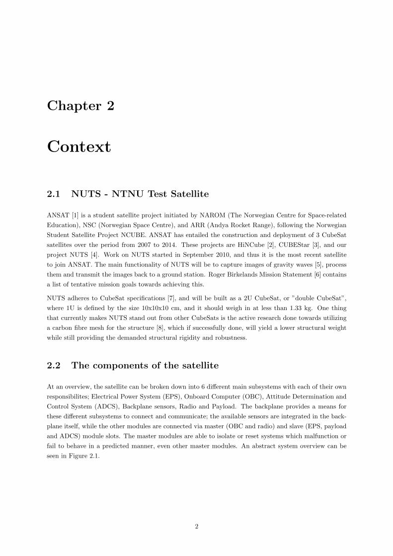
2.2 The components of the satellite

At an overview, the satellite can be broken down into 6 different main subsystems with each of their own

responsibilites; Electrical Power System (EPS), Onboard Computer (OBC), Attitude Determination and

Control System (ADCS), Backplane sensors, Radio and Payload. The backplane provides a means for

these different subsystems to connect and communicate; the available sensors are integrated in the back-

plane itself, while the other modules are connected via master (OBC and radio) and slave (EPS, payload

and ADCS) module slots. The master modules are able to isolate or reset systems which malfunction or

fail to behave in a predicted manner, even other master modules. An abstract system overview can be

seen in Figure 2.1.

2

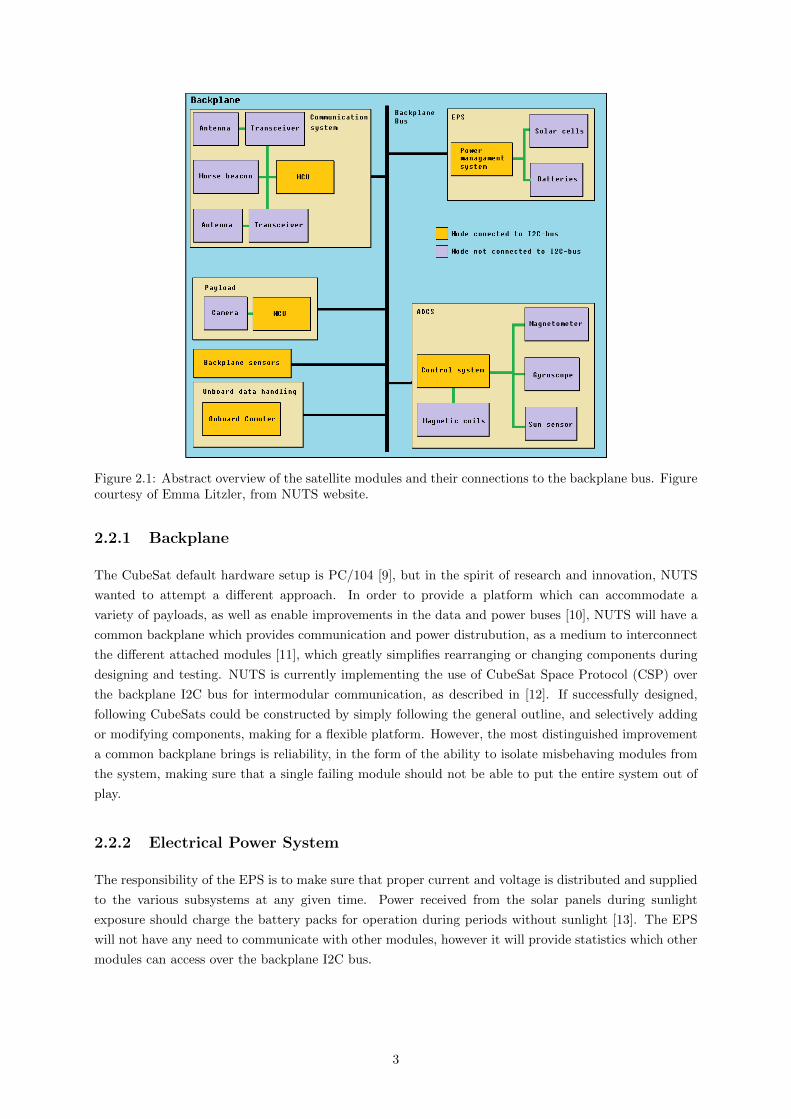
Figure 2.1: Abstract overview of the satellite modules and their connections to the backplane bus. Figurecourtesy of Emma Litzler, from NUTS website.

2.2.1 Backplane

The CubeSat default hardware setup is PC/104 [9], but in the spirit of research and innovation, NUTS

wanted to attempt a different approach. In order to provide a platform which can accommodate a

variety of payloads, as well as enable improvements in the data and power buses [10], NUTS will have a

common backplane which provides communication and power distrubution, as a medium to interconnect

the different attached modules [11], which greatly simplifies rearranging or changing components during

designing and testing. NUTS is currently implementing the use of CubeSat Space Protocol (CSP) over

the backplane I2C bus for intermodular communication, as described in [12]. If successfully designed,

following CubeSats could be constructed by simply following the general outline, and selectively adding

or modifying components, making for a flexible platform. However, the most distinguished improvement

a common backplane brings is reliability, in the form of the ability to isolate misbehaving modules from

the system, making sure that a single failing module should not be able to put the entire system out of

play.

2.2.2 Electrical Power System

The responsibility of the EPS is to make sure that proper current and voltage is distributed and supplied

to the various subsystems at any given time. Power received from the solar panels during sunlight

exposure should charge the battery packs for operation during periods without sunlight [13]. The EPS

will not have any need to communicate with other modules, however it will provide statistics which other

modules can access over the backplane I2C bus.

3

2.2.3 Onboard Computer

The OBC will take on the role as the center of operational control, performing tasks which include [14]:

• Supervising other modules to ensure that they are functioning as intended by executing maintenance

routines.

• Processing and compressing captured data from the payload (IR camera).

• Transferring data to the radio module, to transmit to a ground station.

• Validating and interpreting instructions received from ground station.

2.2.4 Attitude Determination and Control System

In short terms, the main responsibilities of the ADCS are twofold; to ensure that the CubeSat will detum-

ble successfully after deployment, and to make sure that the satellite continuously rotates into a desired

orientation (generally pointing payload towards Earth) while in orbit. Part of this is the responsibility

for collecting information about the positional and rotational state of the satellite, like measuring the

Sun vector, as the main topic of this report will be.

2.2.5 Backplane sensors

The backplane contains multiple simple hardware elements, such as sensors which measures different

physical properties, like temperature or currents. Reading the statistics from one of these elements is

done directly through the I2C-bus. Each of these elements are connected to the bus through a hardware

interface where software functionality is not a possibility [11].

2.2.6 Radio

The inherent responsibility of the radio system is to ensure communication between ground stations and

the satellite, by receiving instructions and returning data. It also provides an outgoing beacon signal

at all times, making sure ground stations can listen in and be able to know when the satellite is in

communications reach. As a master unit on the backplane, the radio is able to reset or isolate other

modules, including the OBC. This ensures resilience to a wide array of possible crashes and bus errors,

and a mutual redundant responsibility with the OBC.

2.2.7 Payload

The responsibilities of the payload module is to acknowledge commands for the capture of IR-pictures,

and executing these [5]. Captured data needs to be transmitted over the backplane I2C bus to the flash

memory on the OBC for processing.

4

2.3 Assignment

2.3.1 Previous work on the ADCS

NTNU have previously launched two CubeSat projects, however unsuccessfully. During these, a lot of

work around the attitude estimation problem has been done, and the topic has undergone iterative changes

and incremental improvements. Svartveit [15] and Ose [16] made work on a discrete Kalman filter, which

was subsequently made into an extended Kalman filter in the work of Rohde [17]. Based on the work of

Psiaki [18] and Markley [19], Jenssen and Yabar [20] made comparisons of the estimation methods used

in the extended Kalman filter, by extending the quaternion estimation (QUEST) method to include non-

vectorized gyroscope measurements and prediction terms, making it more suitable for attitude estimation.

Rinnan [21] developed the EQUEST further, extending it to include attitude predictions and gyroscope

information in the cost function, as well as comparing the developed EQUEST method to a nonlinear

observer and combining the two.

Much of this previous work mentions using solar panels as a crude sun sensor for attitude determination,

however most list further investigation into this possibility as further work, along with that the main

challenge is compensating for the Earth albedo error.

2.3.2 This report

This report aims to give an introductory review of selected sensory technologies available for attitude

determination, and to document the effort of investigating the utilization of solar panel readings for this

purpose on the NTNU Test Satellite. Recognizing the limitations of the previously designed sun vector

generation model, an entirely new theoretical approach has been modeled and investigated. Designs for

experiments to verify the validity of this approach has been made, and MATLAB code to support testing

has been produced. An outline of the possible content of an algorithm for separating relevant inbound

sunlight information from disturbance are discussed.

5

Chapter 3

Preliminaries

3.1 Attitude terminology

Attitude: Orientation of a defined spacecraft body coordinate system with respect to a defined external

frame.

Attitude determination: Real-Time or Post-Facto knowledge, within a given tolerance, of the space-

craft attitude.

Attitude control: Maintenance of a desired, specified attitude within a given tolerance. Information

from attitude estimation and determination enables the attitude control to perform command engineer-

ing functions, like directional pointing of solar panels or antennas, or nadir control for Earth observing

payloads.

Attitude error: Low frequency spacecraft misalignment; usually the intended topic of attitude control.

Attitude jitter: High frequency spacecraft misalignment; usually ignored by ADCS; reduced by good

design or fine pointing/optical control.

3.2 Attitude representations

There are a number of different ways to express the rotations in three dimensional space, and thorough

descriptions of these can be found in most of the Master theses published in relation to the NUTS project,

where the estimation algorithms make great use of quaternion representation due to their suitability for

digital implementation and resilience to singularities. For this report we will not need to express a lot of

complex rotations, as the investigations made for the most part take place in the satellite body frame,

however there will be mentions of roll, pitch and yaw, and some use of simple rotations which can be

expressed in a satisfactory manner through the use of the Euler angles shown below.

6

3.2.1 Euler angles

Described by Leonhard Euler in 1776 [22], this representation of the orientation of a body is arguably the

most convenient and intuitive for a wide field of applications. To fully describe an orientation between

two frames, three parameters are needed; one angle for the rotation around the three frame axes. These

angles are best known under the names of roll, pitch and yaw, and are usually denoted by φ, θ and ψ.

Euler angles are commonly used in the definitions of R3 right hand rule rotation matrices about the x,y

and z-axis, which looks like the following:

Rx(φ) =

1 0 0

0 cos(φ) − sin(φ)

0 sin(φ) cos(φ)

(3.1)

Ry(θ) =

cos(θ) 0 sin(θ)

0 1 0

− sin(θ) 0 cos(φ)

(3.2)

Rz(ψ) =

cos(ψ) −sin(ψ) 0

sin(ψ) cos(ψ) 0

0 0 1

(3.3)

A rotation matrix R is typically used to describe a rotation between two coordinate frames, given three

successive rotations around each single, fixed axis of the frame in order; a rotation ψ around the z-axis,

θ around the y-axis, and φ around the x-axis. The entire rotation can be written as:

Rab = Rz(ψ)Ry(θ)Rx(φ) (3.4)

A given vector in, say, the BODY frame kb can be expressed in the NED frame kn by using a rotation

matrix:

kn = Rnb k

b (3.5)

And for the sake of illustrating the difference between Euler angles and quaternions, here rotations are

represented by quaternions as the following [23] [24]:

R(q) = (q24 − ‖q13‖2)I3×3 + 2q13q13> − 2q4[q13×] (3.6)

which obviously is not as perceptually intuitive, and would hence make a poor choice for this report as it

will attempt to illustrate a new concept in a fashion which should be easy to grasp. We will not go into

what the different components of the quaternions are, or how they are used, but an extensive review can

be found in the work of Rinnan [21].

7

3.3 Reference frames

The following coordinate frames can be involved in describing different aspects of the attitude of the

satellite:

3.3.1 Earth Center Inertial (ECI)

This reference frame is usually applied for orbital analysis of an Earth orbiting satellite, for inertial mo-

tion analysis and astronomy purposes. For these applications the ECI is considered a sufficiently inertial

and non-accelerating reference frame in the sense that its acceleration due to the Earth orbiting the sun

can be disregarded. It consists of a system of celestial coordinates i = [xi yi zi]>, with the positive

x-axis defined to point towards the vernal equinox, γ, which is the point where the sun crosses the Earth’s

equatorial plane when it goes from south north. The z-axis falls in line with the rotational axis of the

Earth, pointing towards the celestial north pole, and the y-axis completes the Cartesian coordinate frame

according to the right hand rule.

3.3.2 Earth Center Earth Fixed (ECEF)

The ECEF frame, e = [xe ye ze]>, use the center of the Earth as its origin, with its x- and y-axis

rotating with the Earth relative to the ECI frame with a rate of ωE = 7.2921 ∗ 10−5[rad/s] about

the z-axis. The positive x-axis is defined to point towards [latitude, longitude] = [0◦, 0◦], which is the

intersection between the Equator and the Greenwich meridian. As with the ECI, the y-axis completes

the frame according to the right hand rule.

3.3.3 North East Down (NED)

This is a local reference frame defined in the tangent plane on the surface of the Earth, with the x-axis

pointing towards north, and z-axis downwards perpendicular to Earth’s reference ellipsoid. The y-axis

completes a right handed orthogonal coordinate system, with the positive y-axis pointing towards East.

Earth’s reference ellipsoid is a mathematically defined surface fitted to approximate the shape of the

Earth, relative to the World Geodetic System

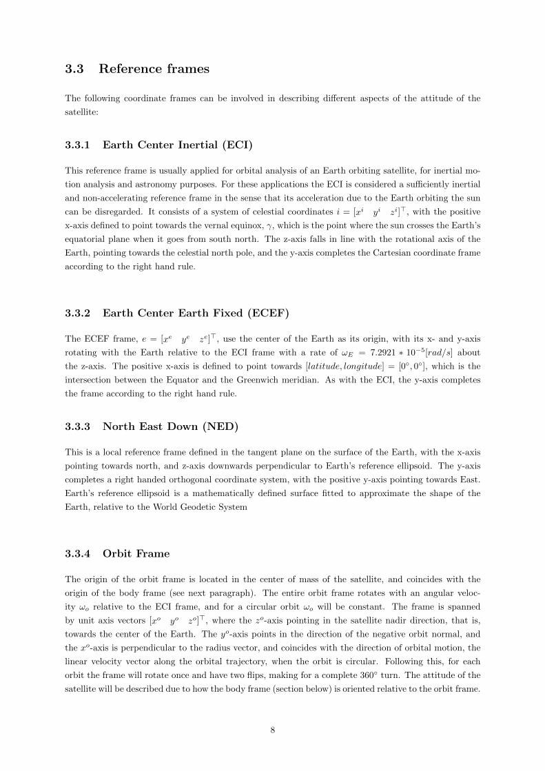
3.3.4 Orbit Frame

The origin of the orbit frame is located in the center of mass of the satellite, and coincides with the

origin of the body frame (see next paragraph). The entire orbit frame rotates with an angular veloc-

ity ωo relative to the ECI frame, and for a circular orbit ωo will be constant. The frame is spanned

by unit axis vectors [xo yo zo]>, where the zo-axis pointing in the satellite nadir direction, that is,

towards the center of the Earth. The yo-axis points in the direction of the negative orbit normal, and

the xo-axis is perpendicular to the radius vector, and coincides with the direction of orbital motion, the

linear velocity vector along the orbital trajectory, when the orbit is circular. Following this, for each

orbit the frame will rotate once and have two flips, making for a complete 360◦ turn. The attitude of the

satellite will be described due to how the body frame (section below) is oriented relative to the orbit frame.

8

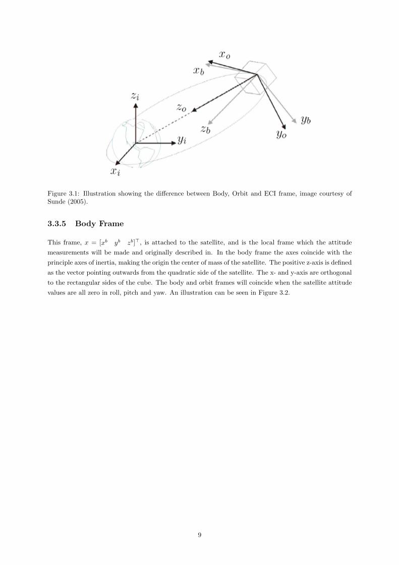
Figure 3.1: Illustration showing the difference between Body, Orbit and ECI frame, image courtesy ofSunde (2005).

3.3.5 Body Frame

This frame, x = [xb yb zb]>, is attached to the satellite, and is the local frame which the attitude

measurements will be made and originally described in. In the body frame the axes coincide with the

principle axes of inertia, making the origin the center of mass of the satellite. The positive z-axis is defined

as the vector pointing outwards from the quadratic side of the satellite. The x- and y-axis are orthogonal

to the rectangular sides of the cube. The body and orbit frames will coincide when the satellite attitude

values are all zero in roll, pitch and yaw. An illustration can be seen in Figure 3.2.

9

Figure 3.2: Illustration of the NUTS Body coordinate system, image courtesy of Jenssen and Yabar(2011).

10

Chapter 4

Available sensors for attitude

determination

Attitude and attitude motion of a spacecraft describes the orientation and rotational motion about its

center of mass, and the computation of this orientation relative to either an inertial reference or some

object of interest is referred to as attitude estimation. This process is necessary in order to provide a

reference for the attitude control system. A commonly used technique is to utilize body measurements to

estimate the vehicle orientation, and comparing these measurements with known reference observations.

Another issue which must be taken into consideration in estimation techniques is the fact that vector

measurements will in practice be contaminated with noise. Especially measurement noise in particular

can contribute a significant factor at high frequencies, making it essential to subsequently filter the noise

by combining the measurements with models. In essence, the key issues in attitude estimation is avoiding

singularities, and providing satisfactory bias estimation [25]

An attitude determination system requires at least two vectors in order to estimate the attitude. The

NUTS CubeSat will contain three types of sensors for the ADCS system; a magnetometer, a sun sensor

and a gyroscope. This report will aim to improve on the model and validity of the calculated inbound sun

vector produced by the sun sensor, however, a brief selection of sensors used for attitude determination

and their abilities will be listed and described here.

Information provided by the sensors is combined and processed in the attitude determination system to

provide the best possible estimates at all times. Sensors commonly used in attitude determination sys-

tems can be divided into two different classes; inertial sensors and reference sensors. Inertial sensors are

sensors that measure rotation or translational acceleration relative to an inertial frame. These sensors

experience random drift and bias errors, and as a result, the errors are unbounded. Regular updates

based on references such as the Sun, stars, or the Earth can be used in order to correct the errors. The

gyroscope is an example of an inertial sensor. Reference sensors typically provides noisy vector observa-

tions at a low frequency [21]. Reference sensors give a vector to some object which position is known.

The rotation between the local body frame, and the frame in which the known vector is given, can then

be computed. With only a single measurement, the rotation around the measured vector is unknown. It

is therefore necessary either to have two different measurements, or to utilize information from the past,

e.g. by using a Kalman filter [15]. An example of such measurement is the angle between the craft and

the Sun, measured with a Sun sensor, or line-of-sight measurements of the position to the stars, provided

11

by a star tracker. These measurements must have a corresponding set of reference vectors in the reference

frame, such as a known Sun reference model, and maps of known observed stars. However, we must keep

in mind that the size and weight requirements of the satellite impose strict limitations on the choice of

sensors. The sensors of choice must be light weight, consume little power, and be of small size. The

vector measurement is a function of spacecraft attitude, but one sample from a reference sensor does not

provide full attitude information. Thus, two vector directions are needed for a complete estimation. Both

the sun sensor and the magnetometer are reference sensors.

4.1 GPS

Mainly three reasons can be pointed out for installing a GPS receiver on board the NUTS CubeSat. First

of all, to determine the attitude of the satellite, the magnetometer measurements will need to be compared

with the IGRF model, hence the need for position data which can be obtained using GPS. When using

the magnetic field for this purpose in the ADCS, it is imperative that the position is known. Second,

using multiple GPS antennas enables for attitude determination using GPS signals, an approach which

was explored in the work of Sundlisaeter [25]. Third, the GPS receiver could be utilized as an additional

payload to measure occultations in the lower atmosphere. However, utilization of a GPS receiver for this

purpose would require a dual frequency receiver, which is not necessary for determining the orbit of the

small satellite. Scientific experiments on occultations in the lower atmosphere was therefore dismissed,

as a dual frequency GPS receiver would cause the already tight budgets of the project to exceed their

limits, in the sense of volume, weight, power, and cost [15].

However, installing a GPS receiver on board a satellite in orbit around Earth is not a straightforward

task. Limitations were imposed by the Coordinating Committee for Multilateral Export Controls (Co-

Com) in the 1960s, with the intention to avoid the use of GPS in intercontinental ballistic missile-like

applications, demanding all GPS devices disabled for any GPS device detected to be traveling at speeds

higher than 1,900 km/h at altitudes higher than 18,000 m. Even though CoCom ceased to function in

1994, most manufacturers still apply these limits to GPS receivers, which disable the unit when either

one or both limits are reached [25] [15].

4.2 Star trackers

One of the most reliable sensors are the Star trackers, since they depend on stars which are orbit indepen-

dent and available anywhere in the sky, and are found used both as single units and in pairs. These are

optical devices which measures the positions of stars relative to the sensor, using photocells or a camera.

They are superior to any other attitude references, and determines attitude within a few arc-seconds of

the true attitude [26]. These sensors require high sensitivity, and are susceptible to a number of errors,

such as that they may easily become confused by reflected or artificial lighting, as well as a number of

optical sources of error. The star sensor compares pictures of star coordinates in the satellite body frame

to a on-board star catalog. The comparing provides a well defined 3-axis attitude representation, such

as the Euler parameters. The sensor may be modeled as the true attitude with added noise [27]. By

using simple geometry it is possible to determine the position of the observer based on which stars the

12

sensor registers. The star sensor is the most accurate attitude sensor, but is also heavier, more expensive,

and require more power than most other attitude sensors. This comes from the fact that star sensors

have extensive computer processing in order to produce their measurements from only a picture. Several

types of star sensors exists, and depending on their method of attitude acquisition they are star scanners,

fixed head star trackers, and gimbaled star trackers. In the past, a main disadvantage of the star sensors

has been their operating range and weight. They had low update rates, and could not operate if the

operating rates became too large, usually 10◦/min [26]. The Danish Technical University (DTU), have

developed a star sensor, µASC, which has greatly increased operating range while decreasing weight and

size [28]. However, a star tracker is still a large and expensive sensor to the extent that it is not feasible

to implement in a CubeSat design such as NUTS, especially when considering the baffle needed to shield

the sensor from Sun-, Earth- and Moonlight.

4.3 Gyroscopes

A gyroscope is an inertial sensor which measures the angular velocity about the sensor axis of the object

to which it is attached, relative to the inertial frame. Gyroscopes can measure rapid changes in the

attitude, and theoretically the satellite orientation can be obtained by integrating the measured angular

velocity. However, in order to be able to provide good estimation, the initialization of the gyroscope need

to be correct, and it is also important that the gyro bias is not too large. Due to the gyro bias, which is

inherent within all gyroscopes, gyroscopes can never be used single handedly in order to obtain attitude

estimates, and they should always be used in conjunction with other sensors [20]. Furthermore, gyro

biases are typically low-dynamic or approximately constant, such that the gyro can track the subject

body orientation up to a certain point. However, the inherent bias of the gyro will cause the attitude

estimates to drift and the gyroscope needs to be calibrated accordingly. The length of time a gyroscope

will provide acceptable measurements can vary. However, most modern gyroscopes provide high quality

measurement data at reasonable cost [25]. The design which is relevant for a project like ours are the

MEMS gyros [29], which is a type of gyros usually based on a tuning fork gyro principle, where a vibrating

fork is subjected to a steady rotation about its axis and the response is detected by the transducer results

from the Coriolis force [30].

4.4 Magnetometers

A magnetometer can only be used in orbit close to earth where the magnetic field is strong and well

modeled. As the NUTS is a Low Earth Orbit (LEO) spacecraft, this is feasible [15]. A magnetometer can

be used to obtain measurements of the flux density of the local magnetic field at the current location of

the satellite. By combining measurements from three mutually perpendicular magnetometers/axes, the

magnetic field including two components of its direction will be given in the body frame when the eventual

rotation between the body and sensor frame is known. By referring to a model or table of known values of

the Earth’s magnetic field, usable estimates of attitude can be made. As the real magnetic field varies in

magnitude and direction with its location and altitude, in addition to slowly changing with time, either an

enormous look-up table would have to be stored on board, or updates would have to be periodically trans-

mitted to the satellite. The drain on time, storage and computational effort this entails made it clear that

NUTS should rather use a mathematical model of the field. The most widely implemented model is the

13

International Geomagnetic Reference Field (IGRF), and this model was implemented on our satellite [31].

The information regarding local magnetic field conditions can also be used as a check on the measurement

accuracy of the carrier phase measurements used by the GPS attitude determination solution method

discussed by Sundlisaeter in [25].

Another issue which arises is that the use of magnetometers and magnetic torque coils are, if not mutually

exclusive during use, a serious local disturbance. Magnetometers are in general susceptible to interference

from spacecraft electronics, which mean that it’s important to consider magnetic radiation and shielding

when implementing satellite hardware and different component orientations in relation to each other [15].

Due to testing done by Busterud [32] which shows that ADCS performance is not degraded by alternating

between measuring and actuating, NUTS aim to handle this by switching between attitude determination

and attitude control, by scheduling the time when the coils are active.

4.5 Accelerometers

Accelerometers, which measures change in velocity, are sensors which seem like a natural choice to include

in inertial navigation systems. The accelerations experienced due to third bodies like the Sun, Moon and

Jupiter, are very small in low Earth orbit, and we can consider the Earth orbit as a celestially isolated case.

The resulting gravitational force is balanced out by the centripetal force, causing a resultant acceleration

of approximately 0 g, which is necessary to keep a stable, circular orbit [20]. In this report we consider

the case where the satellite is in a stable circular orbit around the Earth, meaning that the spacecraft is

in continuous free fall towards the Earth, meaning that net acceleration experienced by the spacecraft in

orbit will be tiny, and regular accelerometers will not be suited for this purpose; although accelerometers

can be used during ground testing, they are not favorable to utilize in a circular orbit [25].

4.6 Earth sensors / Horizon scanners

The Earth is always visible for satellites orbiting it, and with the knowledge of the orbit, a reference may

be acquired anywhere. An Earth sensor, or horizon scanners as they are also known as, determines the

Earths position relative to the satellite. Because of the approximated circular shape of the Earth, only

the roll and pitch part of the Euler angles can be determined from the measurements [26]. This sensor

can for instance be an infrared camera, or an optical instrument that detects the border between the

warm atmosphere and the cold cosmic background radiation. [20]. However, accurate horizon scanners

are relatively big and expensive sensors, and hence not suited for the NUTS [15]. Although, as a practical

example, the LEO satellite SPARTNIK use infrared detectors as Earth sensors, determining the satellite’s

pointing relative to the Earth, and was used for the following purposes:

• As a way to determine when the Earth is in the viewing area of the camera.

• As support for their attitude determination by Earth sensing.

The Earth-horizon sensors consist of two photo transistors whose output is a function of infrared radiation.

As can be seen in Figure 4.1, the infrared detectors are located on the top face of the spacecraft, one

on each side of the camera lens, mounted inside of a aluminum honeycomb structure with an opening of

14

Figure 4.1: SPARTNIK’s Earth Horizon detector

approximately 1 mm through the outer aluminum plate. The purpose of a small aperture is to aid in

limiting the field of view of both sensors. By mounting these sensors in such a way, the Earth will be the

only source of infrared radiation which will occupy the sensors combined field of view of approximately 40

degrees. This is known since at an altitude ranging from 300 to 700 km, the Earth will occupy between

145 to 130 degrees field of view of the camera’s face as it points towards Earth. Considerations must also

be given to the infrared radiation emitted by the moon and the sun. By careful mounting of the sensors, it

can be made reasonable to assume that the Earth will be the only body able to cause a maximum output

from both detectors simultaneously. Calibrations and/or adjustments of available fields of view might

be needed to avoid triggering on excessively wide incidence angles, depending on the sensor makeup and

orientation [33].

4.7 Sun sensors

The Sun provides a reference when the satellite is in line of view of it. Sun sensors are popular, ac-

curate and reliable, but require clear fields of view; the Suns visibility from the satellite is dependent

on orbit, and only in occurrence of an eclipse, the reference availability ceases. Obviously, Sun sensors

can only provide attitude knowledge when in the Sun, which is roughly two thirds of the time for LEO

spacecraft [34]. However, attitude knowledge is most useful in the Sun for many reasons. Pointing solar

arrays is only useful when in the Sun. Also, most missions would utilize attitude determination while the

spacecraft is lit because attitude control, high bandwidth communication, and many payloads require a

large portion of the spacecraft’s power. Power can be stored in batteries, and usually is, but a concept

of operation that pushes the majority of power use to the lit portions of the orbit is more efficient [34].

In principle the Sun sensor is a measurement of the Suns relative position with respect to the satellites

body frame. This position, expressed as a direction by a vector, is called the Sun vector measurement.

A common property in sun sensing equipment is that they tend to have a small size and low mass, a

wide field of view, medium/high accuracy, high reliability and radiation tolerance, all of which are im-

portant for use in a small satellite ADCS system. The typical field of view for a sun sensor is ±30◦,

with an accuracy of approximately 0.01◦ [35]. A sun sensor reference model is needed for the attitude

determination, and such a model is presented in the works of Rinnan [21], using the previous work of

Svartveit [15] and Sunde [26], and will be presented later in this report for the sake the readers continuity.

15

There exist numerous ways of measuring the sun vector. Depending on the mission requirements, a

number of different types of sun sensors may be used. It has been shown that COTS photo diodes can

be used as Sun sensors. Like COTS magnetometers, these sensors are small, inexpensive and require

very little power. They are typically found in the form of concepts such light dependent resistors or

light-to-frequency converters [17]. Sun sensors range from coarse sun sensors such as the Sun acquisi-

tion sensor (SAS) and attitude anomaly detector (AAD), further to the analog fine sun sensor such as

the quadrant sun sensor (QSS), and finally to the digital fine sun sensor (DSS) [26]. Recently, some

solar panel providers specializing on CubeSat components have started offering the integration of fine or

course Sun sensors, like small photo diodes, into the solar panel faces. These components are available

for any side of a CubeSat, in varieties between from 0.5U to 12U. Needless to say, these components are

costly and should not be obtained unless the project is absolutely sure of crucial components of the final

ADCS design, as there is little room for changing things about on these standalone multicomponent parts.

The sun sensors mounted on the satellite will in general be sensitive to every light source in space. Because

of light reflected from the Earth, it is important to use an Earth albedo compensation when computing

a sun vector, or else a large angular deviation might occur [36]. It can be noted that a DSS can have the

tradeoff of a limited field of view, but not be affected by the Earth albedo unless the Earth is adjacent

to the sun from the satellite point of view [37].

The NUTS CubeSat will attempt to utilize the solar cells as sun sensors, seeing as almost the entire

satellite is covered in solar cells, and being able to use these successfully will reduce some weight and

cost for not only this satellite, but also possibly future iterations of the ANSAT CubeSat (or similar)

projects. Not having to sacrifice solar panel surface for external sensors to have a clear line of sight also

means that we do not reduce our power generating capacity and battery charging rate. Solar cells are

not really sensors, but can be used to detect the direction to the Sun by monitoring the output current.

The output from a solar cell depends on the angle between the solar panel and the sun rays, but is highly

susceptible to the Earth albedo disturbance. It can also be mentioned that the problem with having solar

cells on only 5 out of 6 sides of the satellite can be somewhat remedied by for example attaching a light

dependent resistor on the payload carrying surface to determine whether it is pointing towards the sun

or not, although this approach has not been taken into consideration in this report.

16

Chapter 5

Designing a sun vector model

5.1 The solar cell

In short terms solar, or photovoltaic (PV), cells are constructed from materials which turn sunlight into

electricity, and are composed of layers of semiconductors such as silicon. Photons strike the solar cell and

are absorbed within the semiconductor material, which excites the electrons in the semiconductor and

cause a electric DC current to flow.

Figure 5.1: General layout of a solar cell

The output from a solar cell is mostly dependent on the sunlight angle of incidence with the cell and

the intensity of the inbound light. When measuring the output to determine the variables producing it,

current sensors are usually chosen over voltage sensors because variations in current output of the solar

panels are more responsive to the incidence angle of a light source. This leads to the assumption that

the currents I are dependent on the suns angle of attack αmax on the solar panel as

I = Imax sinαs (5.1)

where Imax is the current induced in the solar panels during direct, perpendicular sunlight, αs = π2 .

The experienced light by one panel alone will not necessarily change much with changing angle of at-

17

tack. It is the experienced light of one panel in together with, and in relation to the rest. As the

satellite changes attitude, some panels will get more and more light, while others will get less. Combin-

ing these results from all five solar panels makes it possible to determine the sun vector in the body frame.

5.2 A trigonometric approach

5.2.1 2 dimensions

Figure 5.2: 2D model of inbound sunlight on NUTS cross section. Image adapted from Svartveit (2003)

With the incoming sun vector striking two orthogonal sides of the satellite as seen in Figure 5.2, we can

establish a relationship between the angles of attack in both planes. Given the triangle similarity and

the sum of the two remaining angles in a right triangle, we have

α1 + α2 =π

2(5.2)

which gives us the further trigonometric relation

sin(α1) = sin(π

2− α2) = cos(α2) (5.3)

Assuming both panels have the same maximum output, applying (5.1) to two sides of the satellite, we

get

I1 = Imax sin(α1) (5.4)

I2 = Imax sin(α2) (5.5)

We can find the relation between the current outputs and the angles by dividing (5.4) with (5.5), which

results in

18

I1I2

=Imax sin(α1)

Imax sin(α2)=

sin(α1)

sin(α2)=

sin(α1)

cos(α1)= tan(α1) (5.6)

⇒ α1 = arctan(I1I2

) (5.7)

5.2.2 3 dimensions

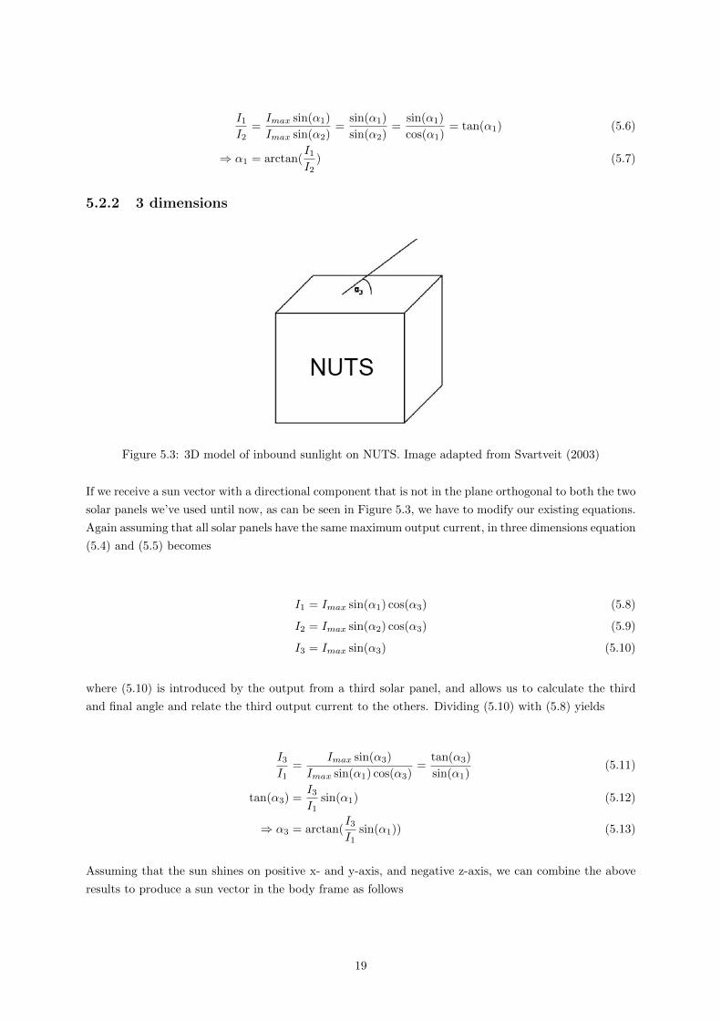
Figure 5.3: 3D model of inbound sunlight on NUTS. Image adapted from Svartveit (2003)

If we receive a sun vector with a directional component that is not in the plane orthogonal to both the two

solar panels we’ve used until now, as can be seen in Figure 5.3, we have to modify our existing equations.

Again assuming that all solar panels have the same maximum output current, in three dimensions equation

(5.4) and (5.5) becomes

I1 = Imax sin(α1) cos(α3) (5.8)

I2 = Imax sin(α2) cos(α3) (5.9)

I3 = Imax sin(α3) (5.10)

where (5.10) is introduced by the output from a third solar panel, and allows us to calculate the third

and final angle and relate the third output current to the others. Dividing (5.10) with (5.8) yields

I3I1

=Imax sin(α3)

Imax sin(α1) cos(α3)=

tan(α3)

sin(α1)(5.11)

tan(α3) =I3I1

sin(α1) (5.12)

⇒ α3 = arctan(I3I1

sin(α1)) (5.13)

Assuming that the sun shines on positive x- and y-axis, and negative z-axis, we can combine the above

results to produce a sun vector in the body frame as follows

19

vBS =

sin(α1) cos(α3)

sin(α2) cos(α3)

− sin(α3)

(5.14)

When seen in comparison with (5.8), (5.9) and (5.10), we get

vBS =1

Imax

I1

I2

−I3

(5.15)

Seeing as Imax is a scalar component which does not contain any information regarding the direction

of the vector, we can discard it. This works well to our advantage, as Imax is directly dependent on

load resistance which hinges on several outside factors, such as which subsystems are in use and battery

status. The sun vector can then be written as

vBS =

X 0 0

0 Y 0

0 0 Z

I1I2I3

(5.16)

where X, Y and Z are ±1 , depending on which of the opposing sides of solar panels are producing power,

which is a restructuring of

vBS =

1 −1 0 0 0 0

0 0 1 −1 0 0

0 0 0 0 1 −1

Intx+

Intx−

Inty+

Inty−

Intz+

Intz−

(5.17)

where Int denotes the intensity of inbound light on each of the corresponding solar panels as demonstrated

in [20]. It can be noted that Intz+ is a void parameter, as this side in particular does not carry a solar

panel, but rather camera equipment.

The main weaknesses of this approach is that we process all inbound sunlight information indiscriminately,

as well as the fact that we have to assume inbound sunlight to originate from negative z-axis in the BODY

frame. This leaves the system wide open to disturbance, and effectively halves our range of sun vector

determination.

5.3 A conical shell model

By the previous approach, we harvest all available incoming sunlight information indiscriminately, and

piece it together in the form of a single sun vector given inbound sunlight angles of all three active solar

panels. A different approach is to treat each solar panel surface as a 2D sensor with a 1D output.

In attempt to combat the weaknesses left by the previous approach, a different model for determining

the inbound sunlight was gradually developed. As spatial trigonometry can be hard to visualize, it was

20

early recognized that a simple physical model was in order, and can be seen in Figure 5.4.

Figure 5.4: Paper model of a 1U CubeSat at 4:5 scale

Looking at the model from different angles for a while made it apparent that by knowing the angles of

inbound sunlight toward just two of the surfaces, it should be possible to produce two different vectors

which would produce an identical output. To put this idea in perspective, a some analogies can be made

to illustrate this concept further:

If we imagine a 2-dimensional vector inbound towards a fixed point on a 1-dimensional solar panel, we

could have two different vectors produce the same inbound 0 − 90◦ angle and thus the same output.

Extending this to a 3-dimensional vector towards a 2-dimensional solar panel results in a conical shell of

possible attack vectors around the axis normal to the solar panel plane, which all will produce the same

angle with the plane, and thus the same output. See Figure 5.5 and 5.6 for illustrations.

Figure 5.5: 2D vectors inbound on 1D panel

When the angle of aperture of these infinite conical shells are large enough, they will intersect with each

other, producing an intersection curve which runs along the conical shells, uniquely defined by the angle

θ about the cones axis of revolution. The thought here is that we should be able to use this information

to derive a common source for the light which produce these angles, in the form of a vector pointing

towards this source. Figure 5.7 illustrates the concept in its most basic state, with two orthogonal,

overlapping panels both experiencing a 45◦ inbound sunlight angle, resulting in two infinite orthogonal

cones with overlapping origins, producing a single common vector which can induce the measured angles.

However, when the combined angles with the planes falls short of 90◦, the cones will intersect in two

lines instead of one, meaning that two different vectors can produce the same angles, like the single

panel in the 1-dimensional case. And when the cones do not share a common origin, they will instead

21

Figure 5.6: 3D vectors inbound on 2D panel

Figure 5.7: 3D vector inbound on two 2D panels

produce an intersection curve, rather than a line. In general terms; when two infinite orthogonal cones

share a common origin (or share their axis of revolution with the axis of a common Cartesian coordinate

system) together possess a total half aperture of 45 degrees or more, they will intersect into each other

and produce an intersection curve along their shell.

5.3.1 With physically accurate origins

To express the problem mathematically, we need to note that our satellite spaces the opposing solar

panels (roughly 5 and 10 cm) away from the center of the satellite, or the origin of the BODY frame.

Seeing as the nature of a solar panel requires the entire panel to receive light in order to produce the

predicted current output, and that all inbound sunlight is parallel, we assume that the panels can be

modeled as a single point somewhere along the axis of the BODY frame. If we were to model the inbound

sunlight angles in the form of infinite conical shells onto two of the solar panel surfaces (YZ and XZ plane

chosen here for demonstration purposes), they would look like this in BODY frame coordinates:

22

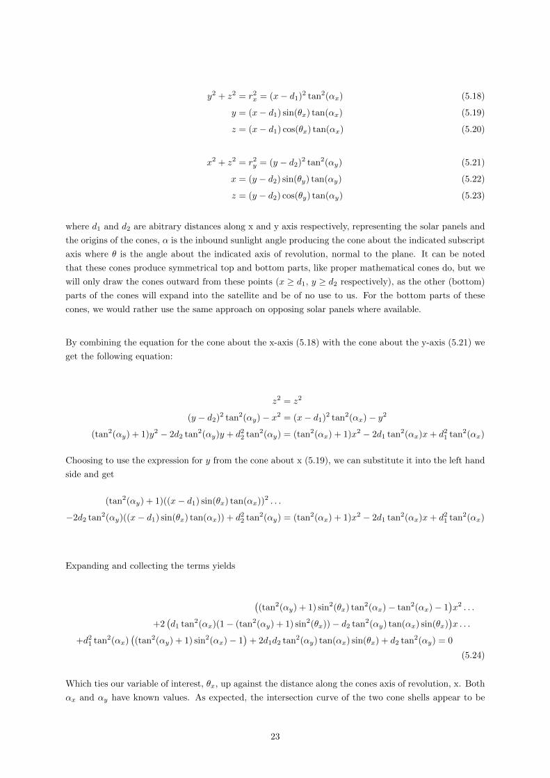
y2 + z2 = r2x = (x− d1)2 tan2(αx) (5.18)

y = (x− d1) sin(θx) tan(αx) (5.19)

z = (x− d1) cos(θx) tan(αx) (5.20)

x2 + z2 = r2y = (y − d2)2 tan2(αy) (5.21)

x = (y − d2) sin(θy) tan(αy) (5.22)

z = (y − d2) cos(θy) tan(αy) (5.23)

where d1 and d2 are abitrary distances along x and y axis respectively, representing the solar panels and

the origins of the cones, α is the inbound sunlight angle producing the cone about the indicated subscript

axis where θ is the angle about the indicated axis of revolution, normal to the plane. It can be noted

that these cones produce symmetrical top and bottom parts, like proper mathematical cones do, but we

will only draw the cones outward from these points (x ≥ d1, y ≥ d2 respectively), as the other (bottom)

parts of the cones will expand into the satellite and be of no use to us. For the bottom parts of these

cones, we would rather use the same approach on opposing solar panels where available.

By combining the equation for the cone about the x-axis (5.18) with the cone about the y-axis (5.21) we

get the following equation:

z2 = z2

(y − d2)2 tan2(αy)− x2 = (x− d1)2 tan2(αx)− y2

(tan2(αy) + 1)y2 − 2d2 tan2(αy)y + d22 tan2(αy) = (tan2(αx) + 1)x2 − 2d1 tan2(αx)x+ d21 tan2(αx)

Choosing to use the expression for y from the cone about x (5.19), we can substitute it into the left hand

side and get

(tan2(αy) + 1)((x− d1) sin(θx) tan(αx))2 . . .

−2d2 tan2(αy)((x− d1) sin(θx) tan(αx)) + d22 tan2(αy) = (tan2(αx) + 1)x2 − 2d1 tan2(αx)x+ d21 tan2(αx)

Expanding and collecting the terms yields

((tan2(αy) + 1) sin2(θx) tan2(αx)− tan2(αx)− 1

)x2 . . .

+2(d1 tan2(αx)(1− (tan2(αy) + 1) sin2(θx))− d2 tan2(αy) tan(αx) sin(θx)

)x . . .

+d21 tan2(αx)((tan2(αy) + 1) sin2(αx)− 1

)+ 2d1d2 tan2(αy) tan(αx) sin(θx) + d2 tan2(αy) = 0

(5.24)

Which ties our variable of interest, θx, up against the distance along the cones axis of revolution, x. Both

αx and αy have known values. As expected, the intersection curve of the two cone shells appear to be

23

a parabola mapping values of θx into values of x. This holds for three dimensional case even if we are

investigating the projection onto the single variable x, as each x, θx pair correspond to a single y and z

value on the intersection curve along the cones. However, what is essential to note about this equation

is that only the lower degrees of the polynomial are depending on the axial offset translations (d1 and

d2) from the BODY reference frame origin. Knowing that a parabolic function approaches a straight line

when moving sufficiently far away from its vertex, we can investigate for which values of θx the function

stops changing, by differentiating (5.24) twice with regard to x:

f(x, θx) = ψ(θx)x2 + β(θx)x+ γ(θx) (5.25)

d2

dx2f(x, θx) = 2ψ(θx)

= 2((tan2(αy) + 1) sin2(θx) tan2(αx)− tan2(αx)− 1

)(5.26)

Where ψ, β, γ in (5.25) replace the corresponding parts of the polynomial, for the sake of readability. We

note that the expression is now only depending on a single variable, θx, and when setting (5.26) equal to

zero we get

2((tan2(αy) + 1) sin2(θx) tan2(αx)− tan2(αx)− 1

)= 0

(tan2(αy) + 1) sin2(θx) tan2(αx) = tan2(αx) + 1

sin2(θx) =tan2(αx) + 1

tan2(αx)(tan2(αy) + 1)

θx = sin−1

(±

√tan2(αx) + 1

tan2(αx)(tan2(αy) + 1)

)(5.27)

where θx are the two symmetrical theta angles about x which the parabolic intersection curve along cones

converges towards as it stretches out towards infinity. It can be noted that θx1 = −θx2.

5.3.2 With coinciding origins

As hinted onto earlier, what is interesting about this is that we can see that the equation for the inter-

secting θx when the cones extend towards infinity will be the exact same as if we were to set d1 and d2

equal to zero, effectively merging the centers/origins of the cones. The difference is that the latter model

will not produce intersecting curves, but rather generate straight lines outward along the intersection,

as long as the combined cone apertures are large enough, which can be seen easily by taking the same

approach to modeling the cones:

24

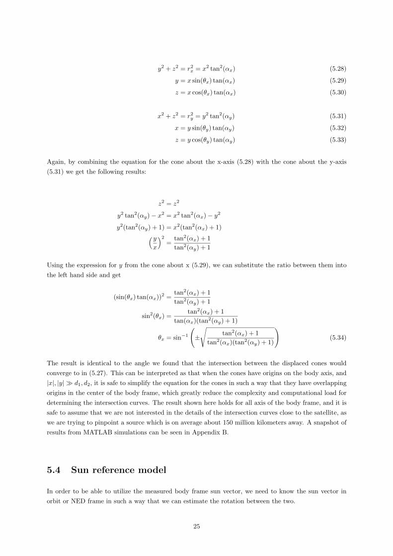
y2 + z2 = r2x = x2 tan2(αx) (5.28)

y = x sin(θx) tan(αx) (5.29)

z = x cos(θx) tan(αx) (5.30)

x2 + z2 = r2y = y2 tan2(αy) (5.31)

x = y sin(θy) tan(αy) (5.32)

z = y cos(θy) tan(αy) (5.33)

Again, by combining the equation for the cone about the x-axis (5.28) with the cone about the y-axis

(5.31) we get the following results:

z2 = z2

y2 tan2(αy)− x2 = x2 tan2(αx)− y2

y2(tan2(αy) + 1) = x2(tan2(αx) + 1)(yx

)2=

tan2(αx) + 1

tan2(αy) + 1

Using the expression for y from the cone about x (5.29), we can substitute the ratio between them into

the left hand side and get

(sin(θx) tan(αx))2 =tan2(αx) + 1

tan2(αy) + 1

sin2(θx) =tan2(αx) + 1

tan(αx)(tan2(αy) + 1)

θx = sin−1

(±

√tan2(αx) + 1

tan2(αx)(tan2(αy) + 1)

)(5.34)

The result is identical to the angle we found that the intersection between the displaced cones would

converge to in (5.27). This can be interpreted as that when the cones have origins on the body axis, and

|x|, |y| � d1, d2, it is safe to simplify the equation for the cones in such a way that they have overlapping

origins in the center of the body frame, which greatly reduce the complexity and computational load for

determining the intersection curves. The result shown here holds for all axis of the body frame, and it is

safe to assume that we are not interested in the details of the intersection curves close to the satellite, as

we are trying to pinpoint a source which is on average about 150 million kilometers away. A snapshot of

results from MATLAB simulations can be seen in Appendix B.

5.4 Sun reference model

In order to be able to utilize the measured body frame sun vector, we need to know the sun vector in

orbit or NED frame in such a way that we can estimate the rotation between the two.

25

A sun sensor reference model, relating the Sun’s position to the satellite orbital position is needed to

be able to utilize the Sun vector measurement in the attitude determination. Rinnan [21] presents such

a model, using the previous work of Svartveit [15] and Sunde [26]. The model assumes a simplification

where the Sun is modeled to revolve around the Earth, making for a geocentric approach. This approach

was demonstrated in the work of Kristiansen to not introduce inaccuracies of noteworthy magnitude [38].

The model will not be utilized in this report, but is presented here for the sake of relevance and continuity.

The elevation of the Sun varies periodically through the year and is given by:

εsun =2π

180sin(

Tsun365

2π) (5.35)

The parameter Tsun is the time in days since the Earth passed the vernal equinox, defined as the spring

equinox as seen from the Northern Hemisphere.

The azimuth angle between the satellite and the Sun is given by:

λsun =Tsun365

2π (5.36)

The time-varying sun sensor reference vector to be used by methods such as the developed EQUEST or

the nonlinear observer is:

r1 := Rθ(εsun)Rψ(λsun)r01 (5.37)

where r01 = [1 0 0]> and the rotation matrices are expressed using Euler angles from (3.2) and (3.3).

26

Chapter 6

Attitude determination testing

6.1 Previous sensor testing

As mentioned earlier, there exists many sensors that can be used for attitude estimation. Due to the

limitations of the NUTS CubeSat with regard to space and weight, which sensors to choose is a question

these factors, as well as the financial budget and a limited power supply. Because of these limitations

sun sensors, gyros and magnetometers were considered a better option than optical devices such as star

trackers and Earth horizon sensors. For the development of attitude estimation methods and prototype

design, the sun sensor was replaced by an accelerometer for testing purposes, due to lack of better testing

options and limited access to components. For the prototype sensor selection, only magnetometers, gyros

and accelerometers were considered. NUTS landed on purchasing and testing several complete Inertial

Measurement Units (IMUs), each with an accelerometer, a gyro and a magnetometer, all with 3 axes.

The three IMUs tested were the Xsens MTi, 9-DOF Razor IMU and CHIMU IMU [20].

The estimation methods used in testing (Extended Kalman filter and EQUEST) each use two indepen-

dent directional vectors and a gyroscope for attitude estimation. Hence, for ground testing on Earth

it is indifferent whether the methods are based on sun sensors measuring the direction to the sun, or

accelerometers measuring the gravitational force on Earth. The only difference will be the input data

and the reference vector for the algorithms. The methods referred to and tested by Jenssen and Yabar

[20] are developed for utilizing an accelerometer, a gyroscope and a magnetometer, but the accelerometer

can easily be replaced by sun sensors producing a reliable sun vector. This is important because, as we

mentioned earlier, an accelerometer is a bad choice to utilize in a circular Earth orbit due to the net

acceleration experienced will be about 0g.

Rinnan [21] continued testing using the 9-DOF Razor IMU, as well as an accelerometer for simulating

sun sensor input.

In the work of Jenssen and Yabar, there is an overview of how to replace the accelerometer measurements

with the hypothetical sun sensor measurements from the trigonometric approach sun vector model. With

some minor alterations, depending on the successful outcome of testing and the final form of the conical

shell sun vector model with what hopefully will prove to be an algorithm to reject disturbance, it too

can be fitted to replace the accelerometer measurements. One might even be able to model the output

from the algorithm to provide values which fits into their suggested implementation of simple directional

27

intensities by injecting it with assumed true intensities computed from rejecting the contribution of cer-

tain inbound light.

6.2 Sun sensor: Conical shell sun vector model

6.2.1 Description

Here can be seen an sequential plan for testing whether or not the conical shell model would hold up in

physical testing against actual current producing solar panels. With the preliminary planning and prepar-

ing done, testing should commence alongside other satellite experiments in January 2013. The readings

should be done in accordance with a fixed, constant intensity light source unless otherwise stated. If the

results from these tests backs up the conical model suggested earlier, further tests utilizing at least one

more panel should be formulated and carried out.

As can be seen in Figure 6.2, a mounting for the purpose of testing two panels simultaneously has been

produced, holding the same prototype solar cells as shown in Figure 6.1. It is precisely 90◦ degrees and

holds the fragile panels in place by double sided adhesive pads, which also ensures that the solar panel

prototypes are mounted flat on the metal surface, with no chance of leakage currents from the circuits.

MATLAB code meant to be used for displaying calculated sun vector from either sequences of data or

real-time data streams can be found in Appendix A.

It should also be mentioned with the future integration of these panels into the EPS in mind, that for

the comparison of the current outputs to be accurate, the solar cells used for sun sensing will have to be

on a common potential. The currently planned layout of the EPS suggests that only one cell on each

face of the satellite will share potential with corresponding cells on the other faces. This possibly means

that we will have to run dedicated wiring to extract the current values from each side of the satellite, to

bring it to the ADCS system.

6.2.2 Testing outline

This section will list a series of incrementally complex tests to see if the conical shell model is realizable.

A testing environment needs to be identified; for these tests, a dark room with a directional light source

should prove sufficient. Also, a means to log current output, preferably in two simultaneous channels

need to be acquired. Measurements either made offline into a structured format, or while connected to

MATLAB through DAQ should prove easiest, as some MATLAB code to interpret a pair of angles into

vectors have been made for simulation purposes. It can easily be modified to transform logged current

levels into registered sunlight angles through the use of the cosine relation between the two.

Test 1: See if output varies with light intensity at a given angle, and if so, how much. Can we define a

saturation level for our test environment by adjusting light intensity or distance from the source? Can

we get same output current by a certain intensity light at one angle, and a different intensity light at a

different angle? In other words, does the light source need to be of a well defined intensity in order for

28

Figure 6.1: Two prototype solar cells on a common board

us to uniquely define the angle by assessing the output current magnitude?

Test 2: Compare simple solar panel model with actual behavior of a single solar panel to see if panel

produce a sinusoidal output given specified angles of inbound sunlight.

Determine Imax and plot current as a function of degrees in two 180◦ sweeps; one along each axis of the

plane spanned by the solar panel. Will probably be easiest to have a fixed light source and rotate the

panel in a controlled manner.

Test 3: Investigate the effect of a disturbance light from an angle wider than the primary light. Does

the intensities accumulate? If they do, do they still accumulate even if the primary source provide light

intensity equal to that of an eventual recorded saturation level?

Test 4: Mount two panels close together with a 90◦ angle between them. Preferably on the outside of

a simple 90◦ angle iron equivalent. Repeat the motions from Step 1 and observe the output. Does one

panel yield max just as the other dies off? Account for discrepancies, possibly such as the fact that our

light source will not be a single point in space.

Test 5: Record the outputs from the dual panel setup at predetermined angles, and if possible record a

smooth transition between two known points in space, both located in the plane spanned by the normals

to the surfaces of the two panels. This should keep the test two dimensional and the produced sun vector

unique. Feed the recorded data (either offline or on the fly) to MATLAB, and convert the current values

into angles which can be sent to the script which draws calculated vectors.

29

Figure 6.2: Two solar cells mounted at a 90◦ angle

Test 6: Repeat step 5, but let the angles be produced from points in space which is not in the plane

spanned by the two surface normals, making the test three dimensional. This should produce ambiguous

readings from the panels, as in that the angles calculated from the current readings should be possible

to produce from light sources at two different points in space. The MATLAB program should illustrate

this by drawing both possible vectors. With the current setup, there will be no way of mathematically

identifying which one is the real vector, and which one is the produced mirror image.

30

Chapter 7

Disturbances and inaccuracies

This part could actually only be named Earth albedo effect, which actually deserves a chapter of it’s own

if one were to really get into the details, however a number of smaller scale elements can be mentioned,

like reflected sunlight off the Moon and the stars in general - which obviously plays a smaller part in the

big picture here. Also, there are several physical factors which can contribute to inaccurate production

of a true Sun vector, like solar panel mounting alignment and cell degradation, which the NUTS team

need to be aware of, but these are not the focus of this report.

7.1 Earth albedo effect

Due to the Earth reflecting energy from the sun, the accuracy of the incoming sun vector can be ques-

tioned. Moreover, only half the Earth is illuminated by the sun at any given time, and the satellite will

regularly have changing parts of this visible in it’s point of view. The albedo also varies greatly from

place to place on the Earth, e.g. the polar areas and sandy areas such as deserts does reflect much more

light than, say, ocean and forest areas.

Appel [36] describes the generation of a model for the light reflected by Earth, using data from the NASA

project Total Ozone Mapping Spectrometer [39] adapted to visible light. From this, patterns showing the

dependencies between latitude, longitude and Earth reflectivity, combined with data averages describing

standard deviations for each latitude provides enough information to randomize reflectivities and create

a statistic reflectivity model of the whole surface of the Earth. From these randomized reflectivities,

polynomial approximations describing the light components in NED frame received by a satellite in an

arbitrary location in orbit can be made by spanning a grid of satellite positions at a given altitude.

Doing this several times yields a statistical model with averages and standard deviations for all three

components, which can produce polynomials describing the intensity of the incoming light as a function

of the satellite latitude and longitude at a certain attitude. The paper concludes with that the model

can drastically improve attitude determination, with a worst case accuracy of 2◦.

31

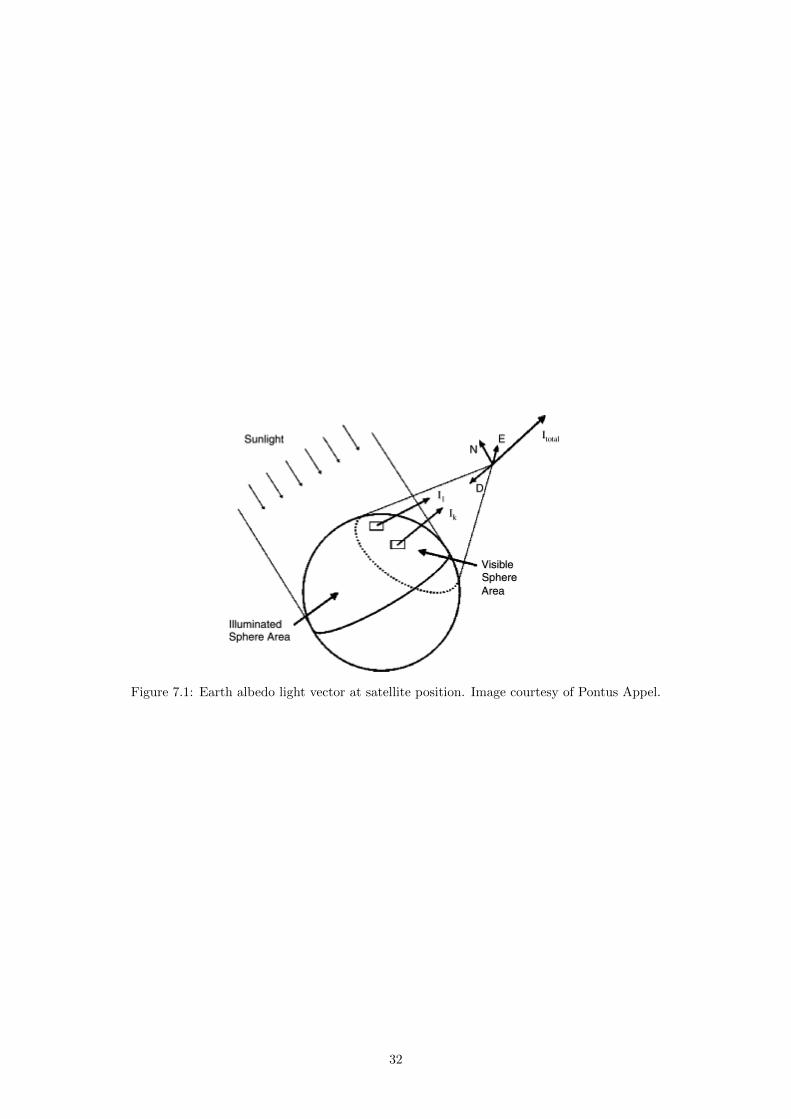
Figure 7.1: Earth albedo light vector at satellite position. Image courtesy of Pontus Appel.

32

Chapter 8

Preliminary disturbance suppression

algorithm

Completing a logic setup which can identify and suppress the Earth albedo effect is beyond the scope

of this report, however a number of observations can be made to help the investigation of the possible

content of an algorithm for separating relevant inbound sunlight information from disturbance.

For the sake of simplifying the illustrations of the ideas in this section, we will assume that we measure

the inbound sunlight continuously rather than sample it at discrete intervals.

It seems reasonable to expect a calculated sun vector to change in a continuous manner, that there should

be no instant jump in the produced vector unless the line of sight with the sun is broken, or a disturbance

suddenly appears. This underlines the beneficial value of keeping track of the history of observed sun

vectors. From this history the rate of change in the orientation of the vector can also be calculated, which

also could prove valuable to utilize for identifying disturbance.

The idea of that the change in sun vector orientation should be smooth can be manifested by identifying

states consisting of combinations of active solar panels which the system should or should not be allow to

transfer between. E.g. the system should not be able to produce sun vectors from output from one panel,

then its opposing panel without registering output from one of the solar panels in between. Though,

the fact that one of the satellite surfaces is not covered in solar panels leaves a number of transitions

unobservable.

In an ideal, disturbance free scenario with solar panels on all six sides, we could formulate the problem

as a system with 27 states in the form of a graph theory inspired cube; 6 faces, 8 vertices, 12 edges and 1

special case where there is absolutely no inbound sunlight. The faces of the cube represent a single active

panel, the edge 2 active panels, and the vertices 3 active panels. Choosing only the three-panel states as

vertices is a design choice given by the fact that these are obviously being the most commonly used state,

as it does not require inbound sunlight to be parallel to any one solar panel plane. The other states may,

for the sake of this representation, be thought of as transitions between vertexes, also known as edges.

Let us call the panels x, y and z, given their respective positions on the satellite BODY axis plane. As

opposing panels can not receive sunlight simultaneously, we can assign them values to show which of the

two are active; x = 1 for sunlight striking the panel on the positive side of the BODY x-axis, -1 for the

opposing one, and 0 for neither. Same with regard to y and z axis panels.

33

Figure 8.1: Visualization of graph inspired state cube, with black vertices and red edges

With these definitions, we can draw the aforementioned graph cube as depicted in Figure 8.1, where the

face [x, y, z] = [1, 0, 0] represents sunlight only hitting the panel on the positive x-axis, and corresponding

for all the other states made from combinations of x, y and z. 33 = 27 is our total number of states, as

expected, where only the 8 different 3-panel states are vertices in the model. What can be noted about

this model, is that transitions between the states should only be allowed in a certain pattern; the system

state can only move from one vertex to one of its three neighboring vertices, and it has to be through the

edge connecting the two (equivalent to 1 Hamming distance if you will, somewhat paraphrased). Also,

through a special case when only a single panel is active, represented by a face on the cube, it can move

to any vertex connected by an edge on the same face. When no panels are active [0, 0, 0], a jump to any

state can occur. This is equivalent to turning off the light, rotating the cube arbitrarily, and turning it

back on again. For the sake of the argument, such a rotation does not necessarily need to be arbitrary

- one might somehow be able to keep track of the satellites rotation during the blackout and calculate

where the sun vector is expected to be when it returns, but this would be well beyond the scope of this

report.

When describing this model, we made some simplifications and assumed ideal conditions, which never is

the actual case. This approach will not be able to identify or compensate for a continuous disturbance,

possibly varying in direction and intensity. And if an approach like this is to be made, either restrictions

will have to be loosened due to the fact that we can not observe the inbound sunlight on the negative

z panel directly, or a compensation will have to be in place, such that we can know the expected value

of this solar panel. What makes this more interesting in the context of this report is that if the conical

shell model approach described in this report should hold up in physical experiments, it should be able

to simulate the output of the missing solar panel.

To be able to separate unwanted information from the incoming sunlight, some logic will have to be

developed, like the idea that we can rule out incoming sunlight that strikes a solar panel on the opposite

panel of where we know the sun to be, meaning if we know all three sides receiving direct sunlight, we can

disregard light which hits the opposing three sides of the satellite entirely, or possibly calculate the effect

of on a third panel by knowing the disturbance that hits two of them. Also, the disturbance hitting a

34

panel which receives direct sunlight should be investigated, as proposed in the testing scheme. If it cause

any reaction at all, it will be in the form of generating additional current, tightening the cone of the panel

in question, which means that two of the intersection vectors will be slightly off, but the redundancy of

the system could possibly limit the effect the disturbance have on the system. In general, the aim will

be to compare generated vectors with each other. In a disturbance free environment, the system should

be able to provide three overlapping vectors, all being true Sun vectors, in addition to the false vectors

which will all be pointing in distances mirrored by the edge between the panels in question, making none

of them overlap. The chance of a high disturbance on more than one active panel is low, as it requires

the satellite to have an unfortunate attitude just as the Sun passes the Earth horizon from the satellite

point of view. If in a scenario with three panels receiving direct sunlight, and one of them receives a

disturbance, which means that it produces a tighter cone due to the higher current level, the panel can

be identified from it’s lack of ability to produce intersections with the other cones. Vectors produced by

Earth albedo influence should have slower rates of change, as the disturbance comes from a wide area,

covering an array of angles in the field of view compared to the single-spot origin of the Sun. And we

should also mention that seeing as the satellite face which carry the camera is supposed to face the Earth,

it should hinder much of the reflected sunlight from Earth from being detected, due to the lack of solar

cells on this side of the satellite. Thoughts like these will need to be expanded upon and combined into a

logic system which can interpret and handle disturbance in a satisfying manner, by hopefully being able

to calculate the amount of a polluted vector reading which is contributed by a source other than the Sun.

35

Chapter 9

Discussion

It may seem ambitious to develop a new, previously untested mathematical approach for something we

can model in a more convenient way by a simple trigonometric approach, so it seems reasonable to ask

ourselves; do we really need this? The answer is, well, both yes and no. What the satellite really do need

is a true, disturbance free Sun vector for the estimation algorithms, which can replace the accelerometer

measurements used during ground testing. Looking at previous theses, this has been suggested over a

number of years without much attention or effort really put into it. What is commonly suggested in

general is a compensation for the Earth albedo effect, which can induce quite large deviances from the

true Sun vector in the readings. This leaves us with two choices, either we carefully make a model of the

reflectivity of the Earth, as described in the work of Appel [36], or what this project has attempted to

undertake - an attempt to make a model which can dynamically compensate for disturbances experienced.

Whether or not it works, the logic derived along this project has sounded reasonable to both the author

and others, so investigating the possibility definitely seemed like a good idea. The mathematical concept

seems promising, even though physical testing and the actual disturbance rejecting algorithm needs to

be attended to.

It should also be mentioned that the actual implementation of the model into the physical system has

yet to be given much thought, so in future development we might run into unforeseen problems such as

sample rate limits, logical corner cases or problems with the actual signals we are trying to measure due

to the load on the batteries/EPS because of other subsystems drawing variable power - it’s hard to tell

at this point really.

36

Chapter 10

Closing remarks

10.1 Conclusion

In this report we have seen a new mathematical model developed for representing sun vectors in the body

frame coordinate system, based on the intersections of conical shells generated by the inbound 3D light

onto the 2D planes spanned by the satellite solar panels. The requirement for two panels to be able to

generate intersecting cones is that the two combined half apertures of the cones, which are depending on

the angle of inbound sunlight, is at least 45◦. This means that the combined angles of inbound sunlight

on the two solar panel planes can not exceed 90◦, as there is no mathematical way for the two panels to

experience a single-point, common light source at these angles.

The simplification of letting the spatially dislocated panels to be modeled as a single point in the center

of the satellite, the origin of the Orbit and Body coordinate frames, lets us model and calculate the

angles about the body frame axes which the intersection curves will converge against when propagating

away from the satellite. This assumption holds as long as we are not interested in the transient phase

of the parabolic intersection curve, which happens close to the satellite. This intersection curve will

approximate a dual sun vector inbound on the body frame origin, of which only one is true, while the

other is a mirror image generated by the inherent ambiguity of the underdetermined system. Through

valid combinations of solar panels, we can potentially calculate 8 different pairs of vectors to describe

inbound light on the satellite, all depending on which sides receive inbound sunlight.

Through enforcing expected rules of behavior of the Sun vector, we should be able to extract and com-

bine information from a selection of panels, and use information from others to negate the impact of

disturbance, or selectively discard information which we know to not carry Sun vector information. En-

suring that observed Sun vector orientation is continuous and, if possible, aligned with measured rotation

from gyroscopes, can make our system less susceptible to introduced disturbances and even help identify

them to use this information to negate their impact. As with the DSS mentioned in Chapter 4.7, Earth

albedo effect experienced when the Sun is close to the Earth from the satellite perspective will be hard

to separate from actual sunlight information. In the end, whether or not this model becomes a feasible

approach to implement on the satellite all hinges on its ability to reject disturbance.

Results from the algorithm processing the currents induced by the measured sunlight should be able to

37

provide filtered readings suitable to insert into the estimation algorithms without having to change too

much of the existing work, as there has already been given thought to how to implement Sun sensor

readings from the trigonometric approach described earlier in this report.

10.2 Further work

Whether or not this mathematical model holds up in physical testing remains to see, the first round of

preliminary testing is laid out and scheduled for January 2013, along other experiments on the satellite

hardware. If the first proof of concept is successful, then extended tests should be planned and carried

out shortly after.

If the necessary testing in a disturbance free environment proves successful enough for the model to

be able to identify isolated single-point light sources, then the real work of establishing a disturbance

rejecting algorithm begins. A general scheme needs to be carefully laid out, and corner-cases which can

confuse the algorithm identified.

Regardless of the success of this particular model, information from the sun sensor needs to replace ac-

celerometer readings alongside IMU measurements for estimator testing, as the satellite will not bring

the accelerometer into space.

38

Bibliography

[1] Ansat, the norwegian student satellite program. Internet. [Online]. Available: http://www.ansat.no

[2] Hincube. Internet. [Online]. Available: http://hincube.com

[3] Cubestar. Internet. [Online]. Available: http://www.cubestart.no

[4] The ntnu test satellite. Internet. [Online]. Available: http://nuts.cubesat.no

[5] M. Bakken, “Signal processing for communicating gravity wave images from the ntnu test satellite,”

Master’s thesis, Norwegian University of Science and Technology, 2012.

[6] R. Birkeland, “Nuts-1 mission statement,” 2011.

[7] Cubesat design specification, California Polytechnic State University Std., Rev. 12, 2009.

[8] K. I. M. Rokstad, “Utvikling av komposittramme for satellitt,” Master’s thesis, Norwegian University

for Science and Technology, 2012.

[9] (2003) Pc/104 specification version 2.5. PC/104 Embedded Consortium. [Online]. Available:

http://www.controlled.com/pc104faq/PC104SpecV2 5.pdf

[10] D. E. Holmstrom, “Databussen i en studentsatellitt,” Master’s thesis, Norwegian University of

Schience and Technology, 2012.

[11] D. D. Bruyn, “Power distribution and conditioning for a small student satellite; design of the nuts

backplane and eps module,” Master’s thesis, Norwegian University of Science and Technology, 2011

2011.

[12] A. Giskeoedegaard, “Implementing csp over i2c on ntnu test satellite,” NTNU, Tech. Rep., 2012.

[13] L. E. Jacobsen, “Power system of the ntnu test satellite; backplane study and design of the eps,”

Master’s thesis, Norwegian University of Science and Technology, 2011.

[14] D. E. Holmstrom, “Software and software architecture for a student satellite,” 2012, pre-project for

masters thesis.

[15] K. Svartveit, “Attitude determination of the ncube satellite,” Master’s thesis, NTNU, 2003.

[16] S. S. Ose, “Attitude determination for the norwegian student satellite ncube,” Master’s thesis,

NTNU, 2004.

[17] J. Rohde, “Kalman filter for attitude determination of student satellite,” Master’s thesis, NTNU,

2007.

[18] M. L. Psiaki, “Attitude-determination filtering via extended quaternion estimation,” Journal of

Guidance, Control, and Dynamics, vol. 23, no. 2, pp. 206–214, Mar.-Apr 2000.

39

[19] F. L. Markley and D. Mortari, “Quaternion attitude estimation using vector observations,” The

Journal of the Astronautical Sciences, vol. 48, no. 2-3, pp. 359–380, Apr.-Sep. 2000.

[20] K. L. Jenssen and K. H. Yabar, “Development, implementation and testing of two attitude estimation

methods for cube satellites,” Master’s thesis, NTNU, 2011.

[21] T. B. Rinnan, “Development and comparison of estimation methods for attitude determination,”

Master’s thesis, NTNU, 2012.

[22] L. Euler, “Formulae generales pro translatione quacunque corporum rigidorum (general formulas for

the translation of arbitrary rigid bodies),” Novi Commentarii academiae scientiarum Petropolitanae,

vol. 20, pp. 189–207, 1776.

[23] P. C. Hughes, Spacecraft Attitude Dynamics. Dover Publications, 2004.

[24] J. Crassidis, F. Markley, and Y. Cheng, “Survey of nonlinear attitude estimation methods,” Journal

of Guidance, Control, and Dynamics, vol. 30, no. 1, January, February 2007.

[25] T. Sundlisaeter, “Spacecraft attitude and orbit estimation using gps and inertial measurements,”

Master’s thesis, NTNU, 2012.

[26] B. O. Sunde, “Sensor modelling and attitude determination for micro-satellite,” Master’s thesis,

NTNU, 2005.

[27] E. Kyrkjeboe, “Three-axis attitude determination using magnetometers and a star tracker,” Master’s

thesis, NTNU, 2000.

[28] Joergensen, Denver, Betto, and Joergensen, “Micro asc - a miniature star tracker,” Small Satellites

for Earth Observation - 4th International Symposium of the International Academy of Astronautics,

pp. 157–162, 2003.

[29] F. S. Holberg, “Design of attitude estimation and control system for a cube satellite,” Master’s

thesis, NTNU, 2012.

[30] B. Vik, Integrated Satellite and Inertial Navigation Systems. Department of Engineering Cybernet-

ics, NTNU, 2009.

[31] Z. Tudor, “Design and implementation of attitude control for 3-axes magnetic coil stabilization of a

spacecraft,” Master’s thesis, NTNU, 2011.

[32] B. E. Busterud, “Orienteringsregulering av mikrosatellitter,” Master’s thesis, NTNU, 2003.

[33] C. Wilkening and Divyesh, “Spartnik microsatellite attitude determination, control and stabiliza-

tion,” San Jose State University, Tech. Rep., 2001.

[34] J. A. Bowen, “On-board orbit determination and 3-axis attitude determination for picosatellite

applications,” Master’s thesis, California Polytechnic State University, 2009.

[35] C. D. Hall, “Spacecraft attitude dynamics and control,” Lecture notes, Department of Aerospace

and Ocean Engineering, Virginia Tech, March 2003.

[36] P. Appel, “Attitude estimation from magnetometer and earth-albedo-corrected coarse sun sensor

measurements,” Acta Astronautica, vol. 56, pp. 115–126, 2004.

[37] F. Boldrini and E. Monnini, “The officine galileo digital sun sensor,” 3rd IAA Symposium on Small

Satellites for Earth Observation, 2001.

[38] R. Kristiansen, “Attitude control of mini satellite,” Master’s thesis, NTNU, 2000.

40

[39] Total ozone mapping spectrometer. NASA. [Online]. Available: http://toms.gsfc.nasa.gov/

41

Appendix A

MATLAB code

1 %draw satellite

2 drawCube([0,0,0],1)

3

4 hold on

5 axis equal

6 axis([-1000 1000 -1000 1000 -1000 1000])

7

8 grid on

9 %box on

10 %axis tight

11 %view([130,30])

12 view([155,30])

13 xlabel(’x-axis’)

14 ylabel(’y-axis’)

15 zlabel(’z-axis’)

16 title(’The graph in three-space.’)

1 function drawCube ( origin, size )

2 x=([0 1 1 0 0 0;1 1 0 0 1 1;1 1 0 0 1 1;0 1 1 0 0 0]-0.5)*size+origin(1);

3 y=([0 0 1 1 0 0;0 1 1 0 0 0;0 1 1 0 1 1;0 0 1 1 1 1]-0.5)*size+origin(2);

4 z=([0 0 0 0 0 1;0 0 0 0 0 1;1 1 1 1 0 1;1 1 1 1 0 1]-0.5)*size+origin(3);

5 for i=1:6

6 h=patch(x(:,i),y(:,i),z(:,i),’w’);

7 set(h,’edgecolor’,’k’)

8 end

9 end

1 function drawCones( alpha_XZ_deg, alpha_YZ_deg )

2 %Function for drawing cones and intersection vectors for

3 %coinciding origin cones produced by input angles of incidence.

4

5 %input light angle calculated by XZ- and YZ-bodyplane solar panel current (0-90 deg)

6 % alpha_XZ_deg = 55;

7 % alpha_YZ_deg = 25;

8

9 %------------------------------------

42

10 %-----Generate cone about X-axis-----

11 %------------------------------------

12 alpha_YZ = alpha_YZ_deg * 2*pi/360;

13

14 %cone aperture halfangle

15 alpha_x = pi/2 - alpha_YZ;

16

17 %discrete running vectors for calculating/displaying

18 x_x = linspace(0,10 ,25);

19 theta_x = linspace(0,2*pi,100);

20 [x_x,theta_x] = meshgrid(x_x,theta_x);

21

22 %calculate z and y based off free variables x and theta about x

23 z_x = x_x.*cos(theta_x)*tan(alpha_x);

24 y_x = x_x.*sin(theta_x)*tan(alpha_x);

25

26 %------------------------------------

27 %-----Generate cone about Y-axis-----

28 %------------------------------------

29 alpha_XZ = alpha_XZ_deg * 2*pi/360;

30 alpha_y = pi/2 - alpha_XZ;

31 y_y = linspace(0,10 ,25);

32 theta_y = linspace(0,2*pi,100);

33 [y_y,theta_y] = meshgrid(y_y,theta_y);

34 z_y = y_y.*cos(theta_y)*tan(alpha_y);

35 x_y = y_y.*sin(theta_y)*tan(alpha_y);

36

37 %------------------------------------

38 %-Calculate intersection theta angles and vectors

39 %------------------------------------

40

41 Tx = tan(alpha_x);

42 Ty = tan(alpha_y);

43

44 theta_x_isct_1 = asin(sqrt((Tx^2 + 1)/(Tx^2*(Ty^2 + 1))));

45 theta_x_isct_2 = pi - theta_x_isct_1;

46

47 v_size = 15;

48 v_1 = [v_size v_size*sin(theta_x_isct_1)*Tx v_size*cos(theta_x_isct_1)*Tx];

49 v_2 = [v_size v_size*sin(theta_x_isct_2)*Tx v_size*cos(theta_x_isct_2)*Tx];

50

51 %------------------------------------

52 %----------------Draw----------------

53 %------------------------------------

54

55 %clear current figure

56 clf

57

58 %set up figure and draw satellite

59 run()

60

43

61 %draw cone 1, about x-axis

62 mesh(x_x,y_x,z_x,x_x)

63

64 %draw cone 2, about y-axis

65 mesh(x_y,y_y,z_y,y_y)

66

67 %draw intersection vectors

68 quiver3(0, 0, 0, v_1(:,1), v_1(:,2), v_1(:,3), ’-b’,’LineWidth’,3)

69 quiver3(0, 0, 0, v_2(:,1), v_2(:,2), v_2(:,3), ’-b’,’LineWidth’,3)

70

71 hold off

72 end

1 function drawConesActual( alpha_XZ_deg, alpha_YZ_deg )

2 %Function for drawing cones and intersection vectors for

3 %spatially dislocated origin cones produced by input angles of incidence.

4

5 %input light angle calculated by XZ- and YZ-bodyplane solar panel current (0-90 deg)

6 % alpha_XZ_deg = 55;

7 % alpha_YZ_deg = 25;

8

9 %------------------------------------

10 %-----Generate cone about X-axis-----

11 %------------------------------------

12 alpha_YZ = alpha_YZ_deg * 2*pi/360;

13

14 %cone aperture halfangle

15 alpha_x = pi/2 - alpha_YZ;

16

17 %discrete running vectors for calculating/displaying

18 x_x = linspace(0.5,800 ,2000);

19 theta_x = linspace(0,2*pi,100);

20 [x_x,theta_x] = meshgrid(x_x,theta_x);

21

22 %calculate z and y based off free variables x and theta about x

23 z_x = (x_x-0.5).*cos(theta_x)*tan(alpha_x);

24 y_x = (x_x-0.5).*sin(theta_x)*tan(alpha_x);

25

26 %------------------------------------

27 %-----Generate cone about Y-axis-----

28 %------------------------------------

29 alpha_XZ = alpha_XZ_deg * 2*pi/360;

30 alpha_y = pi/2 - alpha_XZ;

31 y_y = linspace(0.5,800 ,2000);

32 theta_y = linspace(0,2*pi,100);

33 [y_y,theta_y] = meshgrid(y_y,theta_y);

34 z_y = (y_y-0.5).*cos(theta_y)*tan(alpha_y);

35 x_y = (y_y-0.5).*sin(theta_y)*tan(alpha_y);

36

37 %------------------------------------

38 %-Calculate intersection theta angles and vectors

44

39 %------------------------------------

40

41 Tx = tan(alpha_x);

42 Ty = tan(alpha_y);

43

44 theta_x_isct_1 = asin(sqrt((Tx^2 + 1)/(Tx^2*(Ty^2 + 1))))

45 theta_x_isct_2 = pi - theta_x_isct_1

46

47 v_size = 125;

48 v_1 = [v_size v_size*sin(theta_x_isct_1)*Tx v_size*cos(theta_x_isct_1)*Tx];

49 v_2 = [v_size v_size*sin(theta_x_isct_2)*Tx v_size*cos(theta_x_isct_2)*Tx];

50

51 %------------------------------------

52 %----------------Draw----------------

53 %------------------------------------

54

55 %clear current figure

56 clf

57

58 %set up figure and draw satellite

59 run()

60

61 %draw cone 1, about x-axis

62 mesh(x_x,y_x,z_x,x_x)

63

64 %draw cone 2, about y-axis

65 mesh(x_y,y_y,z_y,y_y)

66

67 %draw intersection vectors

68 quiver3(0, 0, 0, v_1(:,1), v_1(:,2), v_1(:,3), ’-k’,’LineWidth’,3)

69 quiver3(0, 0, 0, v_2(:,1), v_2(:,2), v_2(:,3), ’-k’,’LineWidth’,3)

70

71 hold off

72 end

45

Appendix B

MATLAB plots

46

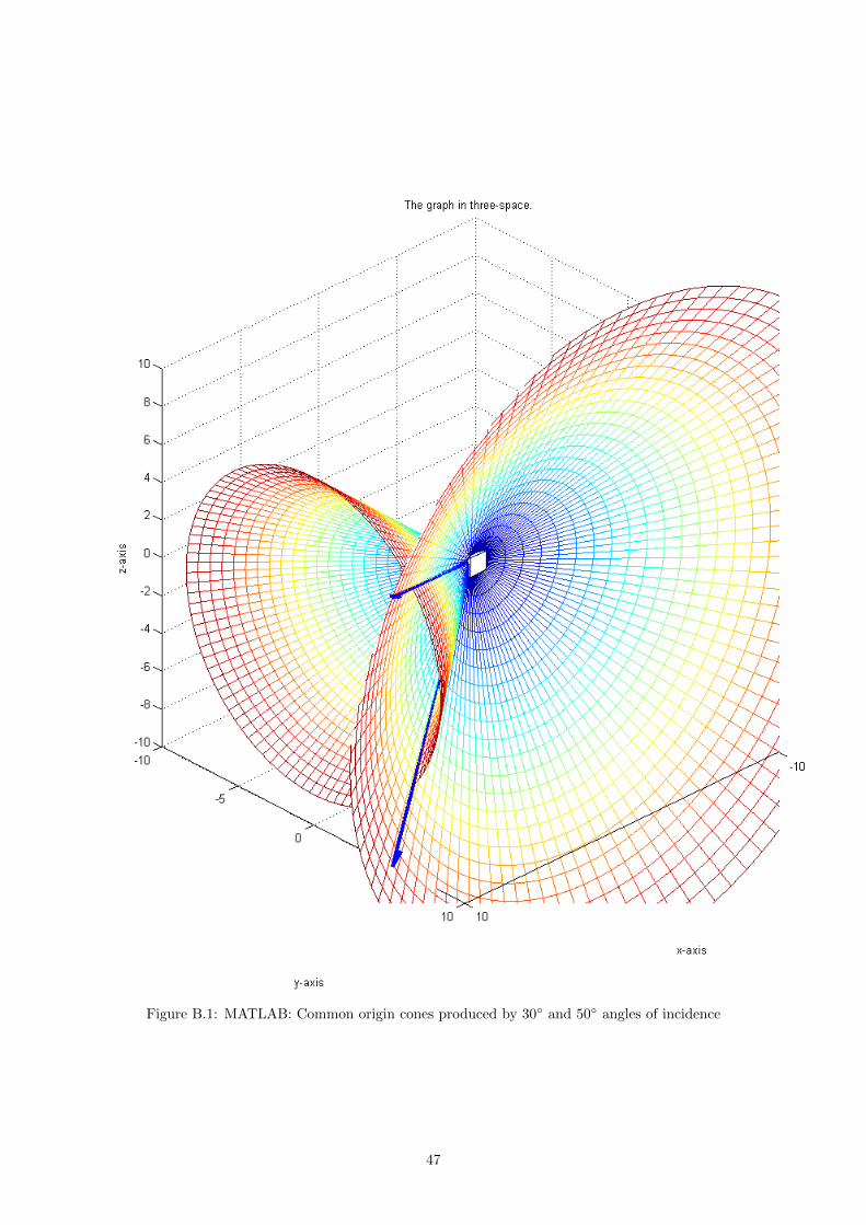
Figure B.1: MATLAB: Common origin cones produced by 30◦ and 50◦ angles of incidence

47

Figure B.2: MATLAB: Separate origin cones produced by 30◦ and 50◦ angles of incidence, far out.

48

Figure B.3: MATLAB: Separate origin cones produced by 30◦ and 50◦ angles of incidence, close in.

49